Abstract
Accurate precipitation forecasting is challenging, especially on the sub-seasonal to seasonal scale (14–90 days) which mandates the bias correction. Quantile mapping (QM) has been employed as a universal method of precipitation bias correction as it is effective in correcting the distribution attributes of mean and variance, but neglects the correlation between the model and observation data and has computing inefficiency in large-scale applications. In this study, a quantile mapping of matching precipitation threshold by time series (MPTT-QM) method was proposed to tackle these problems. The MPTT-QM method was applied to correct the FGOALS precipitation forecasts on the 14-day to 90-day lead times for the Pearl River Basin (PRB), taking the IMERG-final product as the observation. MPTT-QM was justified by comparing it with the original QM method in terms of precipitation accumulation and hydrological simulations. The results show that MPTT-QM not only improves the spatial distribution of precipitation but also effectively preserves the temporal change, with a better precipitation detection ability. Moreover, the MPTT-QM-corrected hydrological modeling has better performance in runoff simulations than the QM-corrected modeling, with significantly increased KGE metrics ranging from 0.050 to 0.693. MPTT-QM shows promising values in improving the hydrological utilities of various lead time precipitation forecasts.
1. Introduction
Meteorological disasters represent one of the most serious types of natural disaster in the world. Among the different kinds of meteorological disasters, a flood disaster induced by heavy precipitation has a wide range of influence, a long duration, and causes significant property loss and casualties [1]. In light of the global warming environment, it is expected that the frequency and intensity of flood disasters will continue to increase [2]. Therefore, there is an urgent need to detect and monitor flood events. Precipitation forecasting is one of the most important and effective tools for obtaining information in flood monitoring [3]. Therefore, if more accurate precipitation forecast information were to be provided before the occurrence of heavy precipitation, this would mark a great contribution to flood forecasting and monitoring and disaster prevention [4,5].
Numerical weather forecast technology has undergone unprecedented development, and the quality of precipitation forecasting has also significantly improved [6], particularly on the short-and-medium-term scale (0–10 days). The effective lead time for a disastrous weather forecast needs to be extended to 14 days through the development of certain skills so as to ensure the significant value of forecasting for decision making [7,8]. However, as the atmosphere is a nonlinear system with inherent randomness [9], there are deviations between the numerical models and the observed data. At the same time, the predictable lead time of a model has a certain range [10]. For example, the predictable lead time of a daily weather forecast is generally around two weeks [11]. In recent years, a series of new random physical process experiments [12] and an updated parameterization scheme [13,14] were designed to improve the model ensemble predictions. However, weather forecasting on the sub-seasonal to seasonal scale is still challenging [15].
Therefore, to obtain accurate and reliable precipitation forecast information and provide a solid foundation for flood forecasting and monitoring, the bias correction of the model precipitation forecast is a significant step. Bias correction is an essential link in the process for obtaining a medium-and-long-term forecast, especially for lead times beyond 14 days. In recent decades, scholars have proved that statistical post-processing methods can effectively reduce or eliminate the systematic errors in the original model data. A variety of bias correction models have been developed based on statistical methods, such as analogs [16,17,18,19], QM, and other non-parametric methods [20,21,22,23,24,25] that are easy to implement and fast to calculate. There are various parametric methods based on complex mathematical and physical models, such as the non-homogeneous Gaussian regression model [26], logistic regression model [27], Bayesian model averaging model (BMA) [28,29], Bayesian joint probability (BJP) [30,31,32], Kalman filtering [33], etc. In recent years, with the development of machine learning technology, this kind of method has been widely used for the bias correction of model data. For example, random forest [34], artificial neural network (ANN) [35,36], convolutional neural network (CNN) [37], and other neural-network-based composite methods [38] have been employed.
QM, as the most efficient method, has been widely used to correct satellite precipitation products and ensemble numerical forecast and general circulation model (GCM) climate forecast data. At the same time, QM can directly calibrate runoff simulations using the hydrological model [39,40,41]. In addition, studies show that assimilating transformed precipitation into the NWP model using QM can also improve the typhoon forecast [42,43]. In the procedure of the QM method, the cumulative distribution function (CDF) of the model data and the observation data are established, respectively. Then, the transfer function (TF) between the two types of data is established for correction, or the model data are directly mapped to the CDF of the observation data [44] to correct the model data. The QM correction method can capture the average evolution of, and variability in, precipitation while adjusting all statistical moments. Many different test schemes based on QM have been successfully applied for bias correction. For example, Terink et al. [45] adjusted the daily RCM simulation precipitation and temperature data of the Rhine River Basin and found that the QM method operated relatively well under normal and extreme conditions. Bennett et al. [20] used QM to correct the annual and seasonal RCM rainfall bias in Australia, and they highlighted that the spatial distribution was improved after bias correction. Similarly, Themeßl et al. [25] found that the QM method effectively corrected the modeled daily precipitation in Alpine areas by analyzing seven bias correction methods. Huang et al. [22] established a five-parameter gamma Gaussian model on the basis of QM, which was successfully used to calibrate the monthly and seasonal precipitation forecasts of GCMS. Although the QM method is effective in correcting distribution attributes such as the mean and variance, the performance of the QM method in optimizing the spatial distribution of forecasting precipitation and detecting the occurrence of precipitation events is not satisfactory. Moreover, the QM method ignores the correlation between prediction data and observation data [41].
Therefore, if the QM method is directly used to correct the forecast precipitation on the sub-seasonal to seasonal scale (14–90 days) with a high temporal resolution (e.g., 3 h), the detailed temporal and spatial characteristics of precipitation will be blurred. In this study, a new bias correction method based on the QM was proposed to calibrate forecasting precipitation on the sub-seasonal to seasonal scale with a high temporal resolution. The new method firstly matches the precipitation threshold according to the time series and then corrects the model precipitation data by QM. The performance of the new bias correction method was analyzed against the observation data and the original QM method in terms of both precipitation accumulation and hydrological simulations.
The remainder of the paper is structured as follows. The datasets and study areas used in this study are described in Section 2. A detailed description of the proposed bias correction scheme is provided in Section 3. The results are presented in Section 4. Section 5 is the discussion and Section 6 is the conclusion.
2. Study Area and Data
2.1. Datasets
The problem of an insufficient spatial distribution of precipitation observed by surface rainfall stations is overcome by satellite remote sensing. Satellite remote sensing precipitation is an important source of precipitation data in many remote areas, particularly in the case of ungauged basins. In 2014, the Global Precipitation Measurement (GPM) was jointly developed by the National Aeronautics and Space Administration (NASA) and the Japan Aerospace Exploration Agency (JAXA) in order to provide high-resolution precipitation data globally. GPM is the inheritance and improvement of the Tropical Rainfall Measuring Mission (TRMM) satellites. On the one hand, the spatial resolution of the precipitation products ranges from 0.25 degree to 0.1 degrees, and the time resolution is increased from 3 h to 30 min. On the other hand, GPM’s dual-band (Ku, Ka) radar system and high-performance microwave radiometer significantly enhance the detection ability for weak rainfall (<0.5 mm/h) and solid precipitation. The core observation platform of GPM is composed of dual-frequency precipitation radar (DPR) and the 13-channel GPM microwave imager (GMI) carried by GPM. DPR is the first type of active spaceborne remote-sensing and dual-frequency rain radar in the world, which is composed of Ku-band radar (13.6 GHz) and Ka-band radar (35.5 GHz). Ku-band radar has a better detection effect for medium-intensive precipitation, and Ka-band radar is more sensitive to small precipitation particles due to its shorter detection band. The GPM IMERG-final product is used as the reference data for analysis in this study. The original temporal resolution of IMERG-final is half-hourly, and the spatial resolution is 0.1 degrees [46]. In this study, IMERG-final was resampled to 0.125 degrees using the arithmetic mean method and accumulated to a three-hourly resolution.
The Flexible Global Ocean–Atmosphere–Land System model (FGOALS) was developed by The Institute of Atmospheric Physics (IAP), Chinese Academy of Sciences (CAS), and the Laboratory of Numerical Modelling for Atmospheric Sciences and Geophysical Fluid Dynamics (LASG) [47]. FGOALS is also one of the coupled models for China’s participation in the 6th International Coupled Model Comparison Program (CMIP6). The output data from the historical climate simulation experiment (2001–2020), based on the updated version of the FGOALS model [48], i.e., FGOALS-f3-L, was used as the model prediction data to be corrected using the new bias correction method on the sub-seasonal to seasonal scale in this study. The FGOALS-f3-L data were interpolated using the first-order conservation interpolation method into 0.125 degrees, consistent with the IMERG-final. The research period of this study was between 2001 and 2020, of which 2001–2015 was the historical period for the experimental data, and the period of 2016–2020 was set as the verification period.
2.2. Study Area
The Pearl River is one of the seven major rivers in China. The Pearl River flows through Yunnan, Guizhou, Guangxi, Guangdong, Hunan, Jiangxi, and other provinces (autonomous regions) and the northeast of Vietnam, with a total length of 2214 km and a total drainage area of 453,690 square kilometers. Of this, the PRB in China covers an area of 442,100 square kilometers, and the basin in Vietnam covers an area of 11,590 square kilometers. The PRB is composed of four water systems, including Xijiang River, Beijiang River, Dongjiang River, and the rivers in the Pearl River Delta. The PRB is located in the inland and subtropical climate zone. The average precipitation from April to September is between 600 and 1900 mm, and the runoff of the PRB from April to September accounts for approximately 80% of the annual runoff [49]. The PRB was the main research area of this study, extending eastward to eastern Guangdong and southward to the coastal areas of western Guangdong and southern Guangxi (Figure 1).
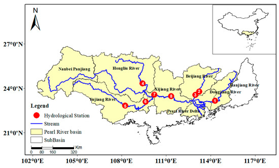
Figure 1.
Research area of PRB in China.
The runoff data of eight hydrological stations in the PRB were selected for this study (Table 1). The time series of the observed runoff data is 2016–2020, and the source of the data is the Pearl River Administration of Navigational Affairs, https://zjhy.mot.gov.cn/zhuhangsj/shuiqingxx/, accessed on 9 May 2021.

Table 1.
Information of main hydrological stations in the PRB.
3. Method
The QM method uses a single transfer function to map the model simulation data to the CDF distribution of the observed data. When the simulated and observed values are relatively close, the revision is better; however, when the difference between the two values is large, the QM method can-not improve the model data significantly and may even introduce new biases. The QM method tends to reproduce the average precipitation from the observation, but the reproducing is not based on the one-by-one mapping between the observation and the model, let alone the correction of the modeled number of wet days [50,51]. In general, the QM method maps all the same precipitation amounts simulated by the model at different times to the same percentile value of observed precipitation, causing exactly the same revised precipitation values.
Manolis et al. [52] used different instances of gamma function that are fitted on multiple discrete segments of the precipitation CDF, instead of the common quantile–quantile approach that uses one theoretical distribution to fit the entire CDF. This allows to better transfer the observed precipitation statistics to the raw model data. However, new uncertainties may be introduced in the CDF fitting using the Gamma-theoretic distribution.
The bias correction methods proposed in this study are described in this section, and the technical workflow is shown in Figure 2a. First, the new bias correction method, which is called the quantile mapping of matching precipitation threshold by time series (MPTT-QM) method, was proposed in this study. A threshold segmentation was performed using different percentiles of historical observed precipitation data [52]. The CDF distribution function of the observed and model data for each interval was then calculated using the nonparametric method of empirical distribution. Four discrimination factors were established according to the threshold distribution characteristics of the observed precipitation in historical periods and the error relationship between the observed and model precipitation. The weighted results of the four discrimination factors were used to determine the threshold intervals of the forecast precipitation, and then the CDF matching method (Figure 2b) was used for further correction within the determined interval.
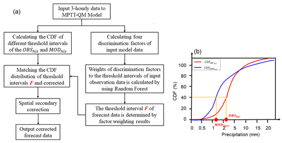
Figure 2.
(a) The workflow of the MPTT-QM method; and (b) the schematic diagram of the QM method. MODfore represents the forecast model data, OBShis represents the mapped observation data by CDF.
3.1. Quantile Mapping of the Matching Precipitation Threshold by Time
The QM method is effective in correcting distribution attributes such as the mean and variance but neglects the correlation between the model and observation data. In this study, the MPTT-QM bias correction model was proposed to solve this problem while retaining the advantages of QM. The percentile method, which is commonly used in precipitation research, was used to determine the threshold interval for this study [53,54]. Specifically, a set of 12 percentile threshold values (i.e., the 10th, 20th,…, 80th, 85th, 90th, 95th, and 98th percentiles) was used to classify all the observed 3-h precipitation data into 13 intervals, similar to those proposed in previous studies [55,56]. For each interval, a list of date–time stamps (referred to as ) for all the observed values was derived as follows:
where () indicates each of the intervals, and indicates the occurrence time when the precipitation intensity falls within the ith interval. The CDF distribution of the observation data in each interval, hereafter referred to as , is calculated. According to , the corresponding model precipitation values (referred to as ) are derived to calculate the model CDF (referred to as ). An initial bias correction is performed using the QM method (Figure 2b):
where represents the forecast model data at a certain time k to be corrected on the sub-seasonal to seasonal scale, and is the corrected results. The problem with the original QM method is that the same precipitation value modeled at different times is mapped onto the same value by the original QM method. To overcome this issue, instead of using the identical CDF function for the bias correction, we propose four discriminant factors in MPTT-QM to adjust the forecast value so as to determine which interval’s CDF matching function should be chosen for the correction. The details of the discriminant factors are described below.
3.2. Discrimination Factors
3.2.1. Discrimination Factor One
The threshold distribution of the observation data (i.e., IMERG-final) is an important reference for estimating the distribution interval of the forecasting threshold. represents the threshold interval with the maximum probability of precipitation distribution at the tth time of a year according to long-term observation. Specifically,
where denotes the number of times when the precipitation values fall in each threshold interval at the same time of the year (i.e., the same month, day, and hour), i denotes the threshold intervals (, and t denotes the 3-h interval time in a year (). is the total number of values falling in the th interval for all the observation times.
3.2.2. Discrimination Factor Two
The error relationship between historical observation and historical model data can be used as an important reference for estimating the distribution interval of the forecasting threshold [23]. The historical precipitation data are extracted at the same time (the same month, day, and hour) as the forecasting precipitation, so that there are fifteen groups in total. The average precipitation in the historical period is defined as the sixteenth group of data. The series of data are written as . The correlation coefficient between the and is calculated, respectively, and the j-group with the largest correlation coefficient is recorded as . One extracts the observation data of the corresponding year of , which is written as . The linear fitting method is used to simulate the error relationship between and [24]:
where and are the linear fitting parameters calculated by the ordinary least squares method. It is assumed that the same error relationship is also followed for future forecast data:
where is the forecast data corrected using the error relationship. The distribution interval of is taken as .
3.2.3. Discrimination Factors Three and Four
The removal of multiplicative errors is a convenient method for bias correction on sub-seasonal to seasonal scales [57]. () represents the forecast threshold interval, with multiplicative error being adjusted as follows:
where is the forecast value to be corrected, is the average value of the observation in the historical period for the same time as the forecast time, and is the average value of the forecast period. The distribution interval of is taken as . The distribution interval of is taken as .
3.2.4. Random Forest
Random forest is a classification algorithm based on a tree classifier, which was first proposed by Breiman [58]. There are many advantages to random forest, for example, it relieves the overfitting problem that often occurs in machine learning. At the same time, the selection of characteristic genes can be carried out. A large number of theoretical and applied studies have proved the accuracy of the random forest model from different angles [59,60]. At present, random forest is considered as one of the best machine learning models due to its tolerance of outliers and noise in the dataset. The contribution weights of different factors to a group of data can be obtained through the random forest model, which is also one of the characteristics of random forest.
In this study, four discriminant factors of each time step in the historical period were used as input data, and the true threshold interval of the historical observation data was used as the target data. Then, the contribution weight of each factor to the true threshold interval of the observed data was calculated through the random forest model.
Above, is the factor, and the weight coefficient of is . The weighted result is the estimated distribution interval of the forecasting threshold. This means that the forecasting data should be matched with the distribution interval F, and the CDF function of the history observation and history model in interval F should be adopted for further correction.
It is critical issue to address the value in the forecast. The method proposed by Tian et al. [61] is adopted in this study. When the forecast precipitation is , the and of the first eight timesteps (one day) of are extracted to calculate the number of missed () and false alarms () of according to . If it is determined that the forecast precipitation is . If the mean value of the first eight timesteps is used to replace the forecast.
3.3. Additional Spatial Correction
In order to maintain better smoothness and continuity of the spatial distribution of the corrected model precipitation data, the outliers need to be removed from the data. Dixon and Dean [62] proposed a simplified outlier test method for smaller sample sizes (), namely the Q-test (or Dixon’s Q-test). This method has been widely used in many scientific research fields, such as international analytical chemistry and materials, for a long time. The calculation of the statistic value is very simple; the difference between the suspicious value and its nearest value is divided by the range. The calculation formula is written as follows:
According to the measured sample number and the given confidence, one can check the critical value table to obtain the value . If (or ) > , there are outliers in the sample data. Otherwise, the data are without any outlier. In this study, we select the spatial window of grid cells (the number of samples ) and gradually slide it to identify outliers. We replace the outlier with the arithmetic mean of the data of the nearest eight non-outlier and non-missing grid cells. That is, a simple interpolation and replacement calculation is performed on the outlier. The outliers among the corrected data are removed by the additional spatial correction. The spatial continuity distribution of the corrected data is better maintained.
3.4. The DRIVE Model
The hydrologic model has been demonstrated to be an effective and efficient tool for monitoring, simulating, and forecasting floods [63,64]. The hydrological simulations were conducted using the Dominant river Routing Integrated with VIC Environment (DRIVE) model, which was developed by Wu [65] through coupling the DRTR (Dominant River Tracing, DRT-based runoff-Routing) model with the VIC (Variable Infiltration Capacity) land surface model. To be applied for spatially distributed and real-time runoff prediction, the VIC model has further been significantly modified (in particular, from its original point-based model structure to a grid-based model structure) so that the modified VIC as a runoff generation component of the DRIVE model is capable of simulating spatially distributed runoff at each time step (i.e., computing all the grid boxes at each time step) [65]. The DRTR model includes a package of hydrographic upscaling (from fine spatial resolution to coarse resolution) algorithms and resulting global datasets (flow direction, river network, drainage area, flow distance, slope, etc.) especially designed for large-scale hydrologic modeling. The DRTR model is grid based and very convenient for simulating spatially distributed streamflow by coupling with the modified VIC model. More details about the DRIVE model can be found in Wu et al. [66]. The DRIVE model has been used routinely for global flood forecasting and monitoring [66], implementing TRMM global satellite precipitation products [67].
3.5. Evaluation Methods
Six precipitation products were used in this study to evaluate precipitation and hydrological performance. They are IMERG-final (IMERG, observation) and FGOALS (model). The FGOALS model precipitation data are corrected by QM and MPTT-QM for 14-day and 90-day lead time forecasts, respectively, which are called QM-14day, QM-90day, MPTT-QM-14day, and MPTT-90day. This also means that the revised calculation is repeated every 14 (90) days. After the completion of each correction process, the observations for these 14 (90) days were summarized into the historical phase dataset, and the initial conditions were recalculated for the next revision.
Firstly, the 3-hourly precipitation products of 2016–2020 were accumulated to daily, 5 days, 15 days, and monthly. Then, the precipitation accuracy was evaluated for each time scale. The model data were assessed through three widely used statistical evaluation metrics: the correlation coefficient (R), root mean square error (RMSE), and mean bias (MB). A higher R, lower RMSE, and absolute MB indicate better agreement between the estimations and observations. The formulas are provided in Table 2. In addition, three indicators were selected in this study to evaluate the precipitation detection capabilities, including the probability of detection (POD), critical success index (CSI), and false alarm ratio (FAR). POD represents the ratio of correct estimates to the number of precipitation occurrences based on observations. FAR denotes the proportion of precipitation occurrences that were erroneously detected. CSI indicates the overall performance in terms of detection capability by integrating POD and FAR. The values of these indicators range from 0 to 1, and a higher POD and CSI and lower FAR indicate a better performance.
Table 2.
Statistical metrics used for evaluating precipitation and runoff estimates. is precipitation estimate; is observation data; is runoff estimate; is observation runoff from the gauge; is the covariance; is the standard deviation and is the mean value; is the number of data pairs; is the number of observed precipitation events detected correctly by the products; is the number of precipitation events detected by the products but not observed; and is the number of precipitation events that the products cannot detect.
Therefore, six different types of precipitation data were used in this study to run the DRIVE model on the 3-hourly time scale and the 0.125-degree spatial scale. The simulated runoff was compared with the runoff observed at eight hydrological stations in the PRB. The Kling–Gupta efficiency coefficient (KGE) was selected as the hydrological assessment indicator. The KGE coefficient is a comprehensive evaluation index integrating the correlation coefficient (R), bias ratio (β), and variability ratio (γ). KGE can comprehensively evaluate the performance of simulation data, and the optimum score is 1.
4. Results
4.1. Precipitation Assessment Results
Figure 3 illustrates the spatial patterns of daily average precipitation from 2016 to 2020, derived from the IMERG, FGOALS, QM, and MPTT-QM precipitation products. It can be seen that the IMERG precipitation in the PRB shows a decreasing trend from east to west. The maximum precipitation area is concentrated in the east of the PRB. The FGOALS model data show a higher value in the eastern area and lower value in the western area. However, the overall precipitation value is smaller than that of IMERG, and there are also great differences in the spatial details. The precipitation products corrected by QM effectively improve the precipitation in the eastern and central areas of the PRB, and QM is more similar to IMERG in terms of spatial distribution. However, the figure shows that the maximum daily rainfall area of IMERG precipitation reaches more than 5 mm/day in the east of the PRB, and there are certain differences between QM-14day and QM-90day, on the one hand, and IMERG, on the other. The precipitation corrected by MPTT-QM is more consistent with the overall spatial distribution of IMERG. It clearly shows four rainbands with decreasing precipitation from east to west. The distribution of MPTT-QM-14day is better than that of MPTT-QM-90day. MPTT-QM-90day has an overestimation trend in the central part of the Pearl River Basin relative to MPTT-QM-14day.
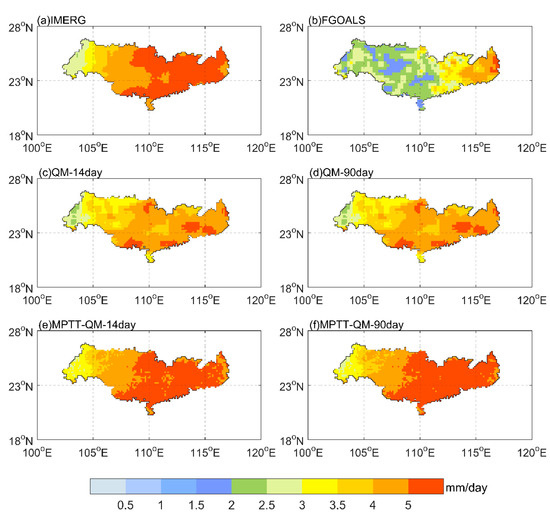
Figure 3.
Spatial patterns of daily average precipitation from 2016 to 2020 in the PRB: (a–f) represent the IMERG, FGOALS, QM-14day, QM-90day, MPTT-QM-14day, and MPTT-QM-90day, respectively.
To further evaluate the spatial distribution consistency between the corrected precipitation and IMERG precipitation, Figure 4 shows a density scatter diagram of the daily average precipitation distribution of each grid cell in the study area. It can be seen from Figure 4a that the FGOALS data show an overall small trend for IMERG. In particular, when the daily average precipitation of IMERG is distributed in the range of 4–5 mm, the FGOALS is as small as 50%. However, for some precipitation maxima, FGOALS shows a higher estimation. The QM-corrected data can effectively solve the problem of the serious underestimation of FGOALS. However, when IMERG precipitation is in the range of 4–6 mm, QM-14day and QM-90day are still slightly low. No matter how high or low the precipitation value is, the scattered points marking the spatial distribution of MPTT-QM and IMERG are basically situated around the y = x baseline, and the performance is clearly better than that of the QM method. As can be seen in Figure 4, there is a more pronounced overestimation trend in MPTT-QM-90day than MPTT-QM-14day when the precipitation level is in the 5 mm interval, which is consistent with Figure 3. In terms of spatial correlation coefficient values and root mean square error values, MPTT-QM-90day and MPTT-QM-14day are very similar, but the spatial mean bias is smaller for MPTT-QM-14day.
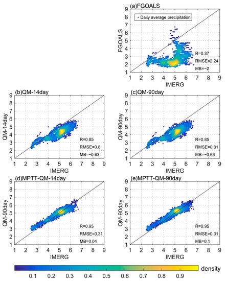
Figure 4.
Density scatter diagram of daily average precipitation of each grid cell relative to IMERG in the PRB from 2016 to 2020. Each scatter point represents the daily average precipitation value of each grid cell in the study area, the color bar represents the density of precipitation values. and (a–e) represent the FGOALS, QM-14day, QM-90day, MPTT-QM-14day, and MPTT-QM-90day, respectively (unit: mm/day).
To verify the time series trend of precipitation on the basin scale, the basin mean values of different precipitation products in the PRB were calculated on the 15-day scale and the monthly scale in this study (Figure 5). The figure shows that the basin mean precipitation of IMERG at 15 days (red line in Figure 5a–e) has changed steadily over the past five years, and the maximum precipitation period is mainly from May to September each year. The three wet years are 2016, 2019, and 2020. Among these, the wet years of 2016 and 2020 were caused by short-term heavy precipitation events, and that of 2019 was caused by continuous precipitation events.
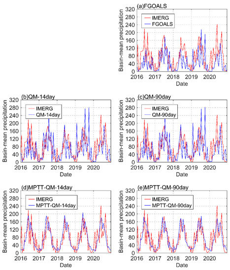
Figure 5.
Time series distribution of average precipitation in the PRB on a half-month scale from 2016 to 2020. The red line represents the IMEGR, and the blue line in figure (a–e) represents the FGOALS, QM-14day, QM-90day, MPTT-QM-14day, and MPTT-QM-90day, respectively (unit: mm).
Regarding the IMERG data, the basin mean precipitation values in the first half of June and August in 2016 and the first half of June and September in 2020 reached 200 mm. The basin mean precipitation in the first half of June 2020 reached 242.24 mm, which is the highest value within the past five years. In Figure 5a, the precipitation of the FGOALS model (blue line) shows a time lag trend and lower precipitation relative to IMERG. Figure 5b,c illustrates that the QM does not have the ability to change the trend of model precipitation. It can only adjust the precipitation value at each time step to make it larger and, therefore, closer to the distribution of IMERG. Moreover, the MPTT-QM model can change the trend of precipitation in the time series (Figure 5d,e). Comparing the MPTT-QM with the QM and FGOALS data, it can be found that MPTT-QM has better consistency with IMERG, especially for 2017, 2018, and 2019. However, for the extreme precipitation events in 2016 and 2020, although MPTT-QM can effectively improve the original data, the correction performance of MPTT-QM for extreme precipitation events still needs to be further improved.
Figure 6 demonstrates the boxplots of R, RMSE, and MB for the MPTT-QM model and other precipitation products over four different time scales. The MPTT-QM model performs better than the other products, with a higher R, lower RMSE, and lower MB. With the increase in the time scale from days to months, the R value becomes higher. However, the daily scale is enhanced to a stronger degree than the monthly scale. For example, for the correlation coefficient R, the median value of FGOALS on the daily scale is 0.02, and the values of MPTT-QM-14day and MPTT-QM-90day are 0.15 and 0.13, which are 650% and 550% higher than the original model data. The monthly FGOALS median value is 0.33, and the MPTT-QM-14day and MPTT-QM-90day are 0.78 and 0.76, respectively, which are 136% and 130% higher than the value for FGOALS. For the QM precipitation products, the performance of R and RMSE is equivalent to that of FGOALS, and there is no significant improvement. On the daily scale, the performance of R and RMSE are slightly decreased. MB is effectively improved using the QM method. The median value of MB is increased from −2.19 to −0.66 (QM-14day) and −0.66 (QM-90day), respectively, on the daily scale. Meanwhile, the median of MB of the MPTT-QM model performed better, with values of 0.07 (MPTT-QM-14day) and 0.13 (MPTT-QM-90day) on the daily scale, respectively. Overall, in terms of time distribution, MPTT-QM-14day outperform MPTT-QM-90day significantly.
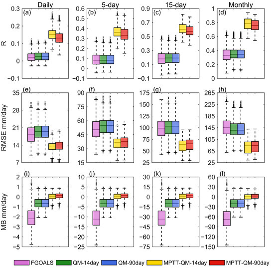
Figure 6.
Boxplots of correlation coefficient (R), root mean square error (RMSE), and mean bias (MB) for five precipitation products over four different time scales: daily, 5-day, 15-day, and monthly. (a–d) represent the boxplot of R, (e–h) represent the boxplot of RMSE, and (i–l) represent the MB.
Table 3 summarizes the statistical metrics of the five precipitation products. The values in the table are the basin average values of the statistical metrics for the PRB on a daily scale. Although the FAR values of MPTT-QM-14day and MPTT-QM-90day are slightly higher, other indicators should be comprehensively considered. Combining the results of several assessment indicators in Figure 4 and Figure 6 in terms of temporal and spatial distribution, the performance of the revised product decreases significantly as the prediction time increases. Overall, the MPTT-QM-14day shows the best performance among the five precipitation products, with POD of 0.950. The second-best-performing product is MPTT-QM-90day, which has the highest CSI value.
Table 3.
Summary of performance statistical metrics for the FGOALS, QM-14day, QM-90day, MPTT-QM-14day, and MPTT-QM-90day precipitation products. The precipitation threshold is set to 0.1 mm/day.
It is worth mentioning that the POD values of MPTT-QM-14day and MPTT-QM-90day are greater than 90% for all grid cells in the PRB. For MPTT-QM-14day, 49.6% of the total grid cells in the PRB have POD values greater than 0.95, and 40% have POD values greater than 0.95 for MPTT-QM-90day. The MPTT-QM-14day and MPTT-QM-90day methods effectively improve the value of CSI by more than 0.4, increasing from 3.6% to 95.3% and 95.1%, respectively.
4.2. Hydrological Assessment Results
First, six precipitation products were used to run the DRIVE model. The KGE coefficient results obtained by comparing the runoff observation data of the hydrological stations on the monthly scale are shown in Figure 7. The runoff simulation results show that the calibrated DRIVE model is efficient. The runoff results of IMERG-DRIVE show that the KGE coefficients of the eight hydrological stations in the PRB are more than 0.48, and there are five stations with monthly KGE values greater than 0.60 (Figure 7). The average of the monthly KGE coefficient is 0.59. Among the stations, the Nanning station data are simulated best, and the monthly KGE coefficient reaches 0.66. The simulation effect of FGOALS-DRIVE on the PRB is unsatisfactory. The average of the monthly KGE coefficient is 0.01. These unsatisfactory results are related to the poor self-quality of the FGOALS precipitation. After QM bias correction, the effect of the runoff simulation was slightly improved. The monthly KGE average increased to 0.16 (QM-14day) and 0.15 (QM-90day), respectively. However, the runoff simulation results of QM still fall short of the credible standard. According to the results of the MPTT-QM-14day runoff simulation, there are five hydrological stations with monthly KGE values greater than 0.4 in the PRB, and the average value reaches 0.45. The performance of MPTT-QM-90day is slightly worse, the average value reaches 0.40. The performance of the MPTT-QM method in hydrology is more related to the self-quality of the observed precipitation.
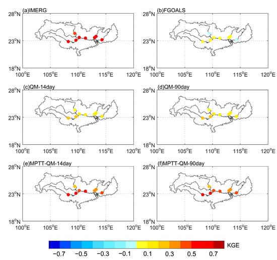
Figure 7.
Spatial distribution of the monthly KGE coefficients of hydrological stations in the PRB: (a–f) represent the IMERG, FGOALS, QM-14day, QM-90day, MPTT-QM-14day, and MPTT-QM-90day, respectively.
On the daily scale, the average correlation between the output runoff data of IMERG-DRIVE and the observed runoff data is 0.74, indicating that the data are highly correlated (Figure 8a). The average correlation coefficient of FGOALS-DRIVE is 0.19, and Nanning station has the highest correlation, which is 0.23. The average correlation coefficients of both QM-14day and QM-90day are 0.16 on the daily scale, a value which is slightly lower than that of FGOALS. The runoff correlation was significantly improved by the MPTT-QM method. After MPTT-QM-14day correction, the correlation coefficients of seven hydrological stations were greater than 0.4. Wuzhou station, located in the middle of the PRB, has the highest correlation coefficient, which reaches 0.60. On the monthly scale, MPTT-QM-14day performed better, raising the average correlation coefficient of FGOALS on the monthly scale from 0.37 to 0.71. Therefore, by comprehensively comparing the KGE coefficient and correlation coefficient of QM and MPTT-QM relative to the observed runoff, it can be seen that the MPTT-QM method is more effective than the QM method.
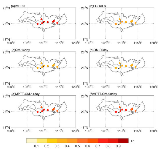
Figure 8.
Spatial distribution of daily correlation coefficients (R) of hydrological stations in the PRB: (a–f) represent the IMERG, FGOALS, QM-14day, QM-90day, MPTT-QM-14day, and MPTT-QM-90day, respectively.
The KGE coefficients of area rainfall of the upstream basin and simulated runoff for the five precipitation products, compared with IMERG, are shown in Table 4. In general, the performance of MPTT-QM in estimating precipitation and runoff of the eight stations in the PRB is significantly better than that of QM method. The MPTT-QM-14day is the best-performing model. For the MPTT-QM-14day model, the average KGE coefficient of the area rainfall compared with FGOALS is increased by nearly 3.82 times, and the average KGE coefficient of the runoff is increased by more than 12.94 times for the eight hydrological stations in the PRB. For the MPTT-QM-90day model, the average KGE coefficients of area rainfall of the upstream basin and runoff are increased by 3.78 times and nearly 12.60 times, respectively. The same conclusion is obtained using the QM method. According to the KGE coefficient of QM-14days, the average rainfall value of the eight stations is doubled, and the average runoff value is increased by nearly 5.03 times. The KGE coefficient of QM-90day is nearly doubled and increased by 4.98 times. It can be seen that both QM and MPTT-QM perform better for the 14-day lead time forecast than 90-day one. Although the KGE coefficient of the area rainfall is higher, both the MPTT-QM and QM bias correction methods are clearly more efficient in improving the runoff simulation.
Table 4.
Summary of performance based on the monthly KGE coefficients of hydrological stations in the PRB for the FGOALS, QM-14day, QM-90day, MPTT-QM-14day, and MPTT-QM-90day. For a hydrological station, P represents the KGE coefficient of model-simulated area rainfall of the upstream basin compared with IMERG. Q. represents the KGE coefficient of model-simulated runoff compared with the IMERG-DRIVE-simulated runoff.
Figure 9 shows the monthly runoff intensity–time curve after the removal of the missing values of the Guigang, Nanning, Wuzhou, and Liuzhou stations in the PRB from 2016 to 2020. The figure shows that the runoff curve (red) simulated by IMERG-DRIVE is closely matched with the distribution of the observation data for most time periods. The runoff value of FGOALS-DRIVE is very small for all the hydrological stations. The QM-DRIVE-simulated runoff data are similar to the precipitation, which is corrected by QM. Only the numerical value can be changed, and it is difficult to change the trend of the runoff. The runoff data simulated by MPTT-QM-DRIVE at four stations show a good performance, which is basically consistent with the runoff intensity–time curve of IMERG-DRIVE.
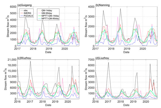
Figure 9.
Runoff intensity–time curve of the PRB on the monthly scale from 2016 to 2020: (a–d) represent the Guigang, Nanning, Wuzhou, and Liuzhou stations, respectively.
Figure 10 illustrates the intensity–time curve of the monthly area rainfall of the upstream basin for the Guigang, Nanning, Wuzhou, and Liuzhou stations. The figure demonstrates that the variation in area rainfall is more complex relative to the runoff. The area rainfall of the upstream basin for the four stations obtained by the MPTT-QM method also indicates a good performance.
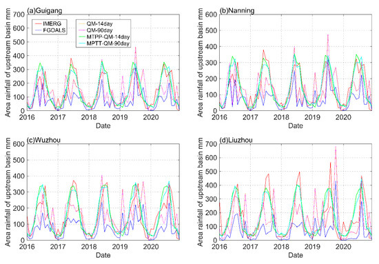
Figure 10.
Area rainfall of the upstream basin intensity–time curve of the PRB on the monthly scale from 2016 to 2020: (a–d) represent the Guigang, Nanning, Wuzhou, and Liuzhou stations, respectively (unit: mm).
5. Discussion
In general, the MPTT-QM-corrected precipitation data indicate a significantly better performance than that of the original QM method in terms of the consistency of the temporal and spatial distribution on the sub-seasonal to seasonal scale. This is because MPTT-QM overcomes the problem that the same precipitation value modeled at different times is mapped onto the same value using the original QM method by correction at the precipitation threshold intervals. In order to more accurately identify the threshold intervals of the forecast precipitation, the four discrimination factors are selected to comprehensively consider the threshold distribution characteristics of the observed precipitation in the historical period and the error relationship between the observed precipitation and the model precipitation.
At the same time, due to the fact that precipitation errors can be transmitted using the hydrological model, more accurate precipitation data will also lead to an improvement of the hydrological simulation performance. Therefore, the MPTT-QM method also has an excellent performance in hydrological simulations.
When the MPTT-QM model is applied in practice, it will provide a solid foundation for the prediction and early warning of flood disasters. At the same time, the MPTT-QM model also requires further improvement. For example, the performance of the MPTT-QM model will decrease slightly with the lead time increase in the bias correction. Moreover, the question of how to predict and correct the occurrence of extreme precipitation events using the MPTT-QM model is the primary problem to be solved in the next stage of model research and development.
6. Conclusions
In this paper, we proposed a new precipitation bias correction method based on QM to match precipitation thresholds by time series, which is called the MPTT-QM model. FGOALS model data were used to estimate 3-h precipitation in the PRB at a spatial resolution of 0.125 degrees. The model performance and retrieval results are summarized as follows:
- The MPTT-QM model has better consistency with IMERG than the original QM model in terms of spatial distribution. The MPTT-QM model excelled in terms of the RMSE and MB;
- MPTT-QM can effectively optimize the change in the precipitation series and improve the correlation coefficient between the model and observation data, which the QM method cannot achieve to any meaningful extent. For a 14-day lead time forecast, MPTT-QM increases the average correlation coefficient of the PRB by nearly six times compared to the original FGOALS model on the daily scale;
- MPTT-QM also shows a stable performance in terms of the POD and CSI. MPTT-QM shows a good precipitation detection ability for the 14-day to 90-day lead time forecasts;
- Based on the hydrological performance evaluation, the KGE coefficients of the eight hydrological stations are improved significantly using the MPTT-QM-DRIVE model compared to the QM-DRIVE model.
Author Contributions
X.L. and H.W. conceived and designed the methods and frameworks; X.L. completed the experiments and wrote the paper; N.N. and H.W. helped to edit the paper. Y.H. and L.L. helped analyze the results; S.C. provided funding support. All authors have read and agreed to the published version of the manuscript.
Funding
This study was supported by the National Natural Science Foundation of China (Grants: 42088101, 42275019, U1811464), and also partially supported by the Program for Guangdong Introducing Innovative and Entrepreneurial Teams (Grants: 2017ZT07X355, 2020B1212060025), the Key R&D Program of Guangxi (Guike AB21075008) and Hainan R&D Program (CXFZ2022J074). The authors would like to thank the anonymous reviewers for their constructive suggestions.
Data Availability Statement
Please contact the corresponding author for the method code and data referenced in this publication.
Acknowledgments
The authors thank the China Meteorological Administration (CMA), Institute of Atmospheric Physics, Chinese Academy of Science, and the National Oceanic and Atmospheric Administration (NOAA) for providing the datasets.
Conflicts of Interest
The authors declare no conflict of interest.
References
- Cross, R. International federation of red cross and Red Crescent Societies. Personnel 2003, 1, 754. [Google Scholar]
- Pachauri, R.K.; Allen, M.R.; Barros, V.R.; Broome, J.; Cramer, W.; Christ, R.; Church, J.A.; Clarke, L.; Dahe, Q.; Dasgupta, P. Climate change 2014: Synthesis report. In Contribution of Working Groups I, II and III to the Fifth Assessment Report of the Intergovernmental Panel on Climate Change; IPCC: Geneva, Szwitzerland, 2014. [Google Scholar]
- Pappenberger, F.; Bartholmes, J.; Thielen, J.; Cloke, H.L.; Buizza, R.; de Roo, A. New dimensions in early flood warning across the globe using grand-ensemble weather predictions. Geophys. Res. Lett. 2008, 35, L10404. [Google Scholar] [CrossRef]
- Fritsch, J.M.; Carbone, R. Improving quantitative precipitation forecasts in the warm season: A USWRP research and development strategy. Bull. Am. Meteorol. Soc. 2004, 85, 955–966. [Google Scholar] [CrossRef]
- Schumacher, R.S. The studies of precipitation, flooding, and rainfall extremes across disciplines (SPREAD) workshop: An interdisciplinary research and education initiative. Bull. Am. Meteorol. Soc. 2016, 97, 1791–1796. [Google Scholar] [CrossRef]
- Vitart, F. Monthly forecasting at ECMWF. Mon. Weather Rev. 2004, 132, 2761–2779. [Google Scholar] [CrossRef]
- Keenan, T.; Joe, P.; Wilson, J.; Collier, C.; Golding, B.; Burgess, D.; May, P.; Pierce, C.; Bally, J.; Crook, A. The Sydney 2000 world weather research programme forecast demonstration project: Overview and current status: Overview and current status. Bull. Am. Meteorol. Soc. 2003, 84, 1041–1054. [Google Scholar] [CrossRef]
- Miyakoda, K.; Smagorinsky, J.; Strickler, R.F.; Hembree, G. Experimental extended predictions with a nine-level hemispheric model. Mon. Weather Rev. 1969, 97, 1–76. [Google Scholar] [CrossRef]
- Lorenz, E.N. Deterministic nonperiodic flow. J. Atmos. Sci. 1963, 20, 130–141. [Google Scholar] [CrossRef]
- Lorenz, E.N. Atmospheric predictability as revealed by naturally occurring analogues. J. Atmos. Sci. 1969, 26, 636–646. [Google Scholar] [CrossRef]
- Li, J.; Ding, R. Temporal-spatial distributions of predictability limit of short-term climate. Chin. J. Atmos. Sci 2008, 32, 975–986. [Google Scholar]
- Li, W.; Zhu, Y.; Zhou, X.; Hou, D.; Sinsky, E.; Melhauser, C.; Peña, M.; Guan, H.; Wobus, R. Evaluating the MJO prediction skill from different configurations of NCEP GEFS extended forecast. Clim. Dyn. 2019, 52, 4923–4936. [Google Scholar] [CrossRef]
- Vitart, F. Impact of the Madden Julian Oscillation on tropical storms and risk of landfall in the ECMWF forecast system. Geophys. Res. Lett. 2009, 36, L15802. [Google Scholar] [CrossRef]
- Zhu, Y.; Zhou, X.; Li, W.; Hou, D.; Melhauser, C.; Sinsky, E.; Peña, M.; Fu, B.; Guan, H.; Kolczynski, W. Toward the improvement of subseasonal prediction in the National Centers for environmental prediction global ensemble forecast system. J. Geophys. Res. Atmos. 2018, 123, 6732–6745. [Google Scholar] [CrossRef]
- Guan, H.; Zhu, Y.; Sinsky, E.; Li, W.; Zhou, X.; Hou, D.; Melhauser, C.; Wobus, R. Systematic error analysis and calibration of 2-m temperature for the NCEP GEFS reforecast of the Subseasonal Experiment (SubX) Project. Weather Forecast. 2019, 34, 361–376. [Google Scholar] [CrossRef]
- Delle Monache, L.; Eckel, F.A.; Rife, D.L.; Nagarajan, B.; Searight, K. Probabilistic weather prediction with an analog ensemble. Mon. Weather Rev. 2013, 141, 3498–3516. [Google Scholar] [CrossRef]
- Hagedorn, R.; Buizza, R.; Hamill, T.M.; Leutbecher, M.; Palmer, T. Comparing TIGGE multimodel forecasts with reforecast-calibrated ECMWF ensemble forecasts. Q. J. R. Meteorol. Soc. 2012, 138, 1814–1827. [Google Scholar] [CrossRef]
- Hamill, T.M.; Bates, G.T.; Whitaker, J.S.; Murray, D.R.; Fiorino, M.; Galarneau, T.J.; Zhu, Y.; Lapenta, W. NOAA’s second-generation global medium-range ensemble reforecast dataset. Bull. Am. Meteorol. Soc. 2013, 94, 1553–1565. [Google Scholar] [CrossRef]
- Hamill, T.M.; Whitaker, J.S. Ensemble calibration of 500-hPa geopotential height and 850-hPa and 2-m temperatures using reforecasts. Mon. Weather Rev. 2007, 135, 3273–3280. [Google Scholar] [CrossRef]
- Bennett, J.; Grose, M.; Post, D.; Ling, F.; Corney, S.; Bindoff, N. Performance of quantile-quantile bias-correction for use in hydroclimatological projections. In Proceedings of the MODSIM 2011-19th International Congress on Modelling and Simulation-Sustaining Our Future: Understanding and Living with Uncertainty, Perth, Australia, 12–16 December 2011; pp. 2668–2675. [Google Scholar]
- Devi, U.; Shekhar, M.; Singh, G. Correction of mesoscale model daily precipitation data over Northwestern Himalaya. Theor. Appl. Climatol. 2021, 143, 51–60. [Google Scholar] [CrossRef]
- Huang, Z.; Zhao, T.; Zhang, Y.; Cai, H.; Hou, A.; Chen, X. A five-parameter Gamma-Gaussian model to calibrate monthly and seasonal GCM precipitation forecasts. J. Hydrol. 2021, 603, 126893. [Google Scholar] [CrossRef]
- Li, H.; Sheffield, J.; Wood, E.F. Bias correction of monthly precipitation and temperature fields from Intergovernmental Panel on Climate Change AR4 models using equidistant quantile matching. J. Geophys. Res. Atmos. 2010, 115, D10101. [Google Scholar] [CrossRef]
- Piani, C.; Haerter, J.; Coppola, E. Statistical bias correction for daily precipitation in regional climate models over Europe. Theor. Appl. Climatol. 2010, 99, 187–192. [Google Scholar] [CrossRef]
- Themeßl, M.J.; Gobiet, A.; Heinrich, G. Empirical-statistical downscaling and error correction of regional climate models and its impact on the climate change signal. Clim. Chang. 2012, 112, 449–468. [Google Scholar] [CrossRef]
- Gneiting, T.; Raftery, A.E.; Westveld, A.H.; Goldman, T. Calibrated probabilistic forecasting using ensemble model output statistics and minimum CRPS estimation. Mon. Weather Rev. 2005, 133, 1098–1118. [Google Scholar] [CrossRef]
- Wilks, D.S.; Hamill, T.M. Comparison of ensemble-MOS methods using GFS reforecasts. Mon. Weather Rev. 2007, 135, 2379–2390. [Google Scholar] [CrossRef]
- Raftery, A.E.; Gneiting, T.; Balabdaoui, F.; Polakowski, M. Using Bayesian model averaging to calibrate forecast ensembles. Mon. Weather Rev. 2005, 133, 1155–1174. [Google Scholar] [CrossRef]
- Wilson, L.J.; Beauregard, S.; Raftery, A.E.; Verret, R. Calibrated surface temperature forecasts from the Canadian ensemble prediction system using Bayesian model averaging. Mon. Weather Rev. 2007, 135, 1364–1385. [Google Scholar] [CrossRef]
- Robertson, D.; Shrestha, D.; Wang, Q. Post-processing rainfall forecasts from numerical weather prediction models for short-term streamflow forecasting. Hydrol. Earth Syst. Sci. 2013, 17, 3587–3603. [Google Scholar] [CrossRef]
- Shrestha, D.L.; Robertson, D.E.; Bennett, J.C.; Wang, Q. Improving precipitation forecasts by generating ensembles through postprocessing. Mon. Weather Rev. 2015, 143, 3642–3663. [Google Scholar] [CrossRef]
- Wang, Q.; Robertson, D.; Chiew, F. A Bayesian joint probability modeling approach for seasonal forecasting of streamflows at multiple sites. Water Resour. Res. 2009, 45, W05407. [Google Scholar] [CrossRef]
- Cheng, W.Y.; Steenburgh, W.J. Strengths and weaknesses of MOS, running-mean bias removal, and Kalman filter techniques for improving model forecasts over the western United States. Weather Forecast. 2007, 22, 1304–1318. [Google Scholar] [CrossRef]
- Taillardat, M.; Fougères, A.-L.; Naveau, P.; Mestre, O. Forest-based and semiparametric methods for the postprocessing of rainfall ensemble forecasting. Weather Forecast. 2019, 34, 617–634. [Google Scholar] [CrossRef]
- Herman, G.R.; Schumacher, R.S. Money doesn’t grow on trees, but forecasts do: Forecasting extreme precipitation with random forests. Mon. Weather Rev. 2018, 146, 1571–1600. [Google Scholar] [CrossRef]
- Li, H.; Yu, C.; Xia, J.; Wang, Y.; Zhu, J.; Zhang, P. A model output machine learning method for grid temperature forecasts in the Beijing area. Adv. Atmos. Sci. 2019, 36, 1156–1170. [Google Scholar] [CrossRef]
- Li, W.; Pan, B.; Xia, J.; Duan, Q. Convolutional neural network-based statistical post-processing of ensemble precipitation forecasts. J. Hydrol. 2022, 605, 127301. [Google Scholar] [CrossRef]
- Zhou, S.; Wang, Y.; Yuan, Q.; Yue, L.; Zhang, L. Spatiotemporal estimation of 6-hour high-resolution precipitation across China based on Himawari-8 using a stacking ensemble machine learning model. J. Hydrol. 2022, 609, 127718. [Google Scholar] [CrossRef]
- Liu, L.; Gao, C.; Xuan, W.; Xu, Y.-P. Evaluation of medium-range ensemble flood forecasting based on calibration strategies and ensemble methods in Lanjiang Basin, Southeast China. J. Hydrol. 2017, 554, 233–250. [Google Scholar] [CrossRef]
- Rajczak, J.; Kotlarski, S.; Schär, C. Does quantile mapping of simulated precipitation correct for biases in transition probabilities and spell lengths? J. Clim. 2016, 29, 1605–1615. [Google Scholar] [CrossRef]
- Zhao, T.; Bennett, J.C.; Wang, Q.; Schepen, A.; Wood, A.W.; Robertson, D.E.; Ramos, M.-H. How suitable is quantile mapping for postprocessing GCM precipitation forecasts? J. Clim. 2017, 30, 3185–3196. [Google Scholar] [CrossRef]
- Lien, G.-Y.; Miyoshi, T.; Kalnay, E. Assimilation of TRMM multisatellite precipitation analysis with a low-resolution NCEP global forecast system. Mon. Weather Rev. 2016, 144, 643–661. [Google Scholar] [CrossRef]
- Da, C.; Kalnay, E. Improving Tropical Cyclone Predictions by Assimilation of Satellite-Retrieved Precipitation with Gaussian Transformation. In Proceedings of the AGU Fall Meeting Abstracts, Washington, DC, USA, 10–14 December 2018; p. NG23A–02. [Google Scholar]
- Wood, A.W.; Maurer, E.P.; Kumar, A.; Lettenmaier, D.P. Long-range experimental hydrologic forecasting for the eastern United States. J. Geophys. Res. Atmos. 2002, 107, ACL 6-1–ACL 6-15. [Google Scholar] [CrossRef]
- Terink, W.; Hurkmans, R.; Torfs, P.; Uijlenhoet, R. Bias correction of temperature and precipitation data for regional climate model application to the Rhine basin. Hydrol. Earth Syst. Sci. Discuss. 2009, 6, 5377–5413. [Google Scholar]
- Hou, A.Y.; Kakar, R.K.; Neeck, S.; Azarbarzin, A.A.; Kummerow, C.D.; Kojima, M.; Oki, R.; Nakamura, K.; Iguchi, T. The global precipitation measurement mission. Bull. Am. Meteorol. Soc. 2014, 95, 701–722. [Google Scholar] [CrossRef]
- He, B.; Bao, Q.; Wang, X.; Zhou, L.; Wu, X.; Liu, Y.; Wu, G.; Chen, K.; He, S.; Hu, W. CAS FGOALS-f3-L model datasets for CMIP6 historical atmospheric model intercomparison project simulation. Adv. Atmos. Sci. 2019, 36, 771–778. [Google Scholar] [CrossRef]
- He, B.; Liu, Y.; Wu, G.; Bao, Q.; Zhou, T.; Wu, X.; Wang, L.; Li, J.; Wang, X.; Li, J. CAS FGOALS-f3-L model datasets for CMIP6 GMMIP Tier-1 and Tier-3 experiments. Adv. Atmos. Sci. 2020, 37, 18–28. [Google Scholar] [CrossRef]
- Zhao, Y.; Zou, X.; Cao, L.; Xu, X. Changes in precipitation extremes over the Pearl River Basin, southern China, during 1960–2012. Quat. Int. 2014, 333, 26–39. [Google Scholar] [CrossRef]
- Minville, M.; Brissette, F.; Leconte, R. Uncertainty of the impact of climate change on the hydrology of a nordic watershed. J. Hydrol. 2008, 358, 70–83. [Google Scholar] [CrossRef]
- Wilby, R.L.; Hay, L.E.; Leavesley, G.H. A comparison of downscaled and raw GCM output: Implications for climate change scenarios in the San Juan River basin, Colorado. J. Hydrol. 1999, 225, 67–91. [Google Scholar] [CrossRef]
- Grillakis, M.G.; Koutroulis, A.G.; Tsanis, I.K. Multisegment statistical bias correction of daily GCM precipitation output. J. Geophys. Res. Atmos. 2013, 118, 3150–3162. [Google Scholar] [CrossRef]
- Hyndman, R.J.; Fan, Y. Sample quantiles in statistical packages. Am. Stat. 1996, 50, 361–365. [Google Scholar]
- Zhang, H.; Zhai, P. Temporal and spatial characteristics of extreme hourly precipitation over eastern China in the warm season. Adv. Atmos. Sci. 2011, 28, 1177–1183. [Google Scholar] [CrossRef]
- Bharti, V.; Singh, C.; Ettema, J.; Turkington, T. Spatiotemporal characteristics of extreme rainfall events over the Northwest Himalaya using satellite data. Int. J. Climatol. 2016, 36, 3949–3962. [Google Scholar] [CrossRef]
- Martius, O.; Pfahl, S.; Chevalier, C. A global quantification of compound precipitation and wind extremes. Geophys. Res. Lett. 2016, 43, 7709–7717. [Google Scholar] [CrossRef]
- Navarro-Racines, C.; Tarapues, J.; Thornton, P.; Jarvis, A.; Ramirez-Villegas, J. High-resolution and bias-corrected CMIP5 projections for climate change impact assessments. Sci. Data 2020, 7, 7. [Google Scholar] [CrossRef]
- Breiman, L. Random forests. Mach. Learn. 2001, 45, 5–32. [Google Scholar] [CrossRef]
- Chen, C.; Liaw, A.; Breiman, L. Using random forest to learn imbalanced data. Univ. Calif. Berkeley 2004, 110, 24. [Google Scholar]
- Primajaya, A.; Sari, B.N. Random forest algorithm for prediction of precipitation. Indones. J. Artif. Intell. Data Min. 2018, 1, 27–31. [Google Scholar] [CrossRef]
- Tian, Y.; Peters-Lidard, C.D.; Eylander, J.B.; Joyce, R.J.; Huffman, G.J.; Adler, R.F.; Hsu, K.l.; Turk, F.J.; Garcia, M.; Zeng, J. Component analysis of errors in satellite-based precipitation estimates. J. Geophys. Res. Atmos. 2009, 114, D24101. [Google Scholar] [CrossRef]
- Dixon, W.J. Analysis of extreme values. Ann. Math. Stat. 1950, 21, 488–506. [Google Scholar] [CrossRef]
- Reed, S.; Schaake, J.; Zhang, Z. A distributed hydrologic model and threshold frequency-based method for flash flood forecasting at ungauged locations. J. Hydrol. 2007, 337, 402–420. [Google Scholar] [CrossRef]
- Yilmaz, K.K.; Adler, R.F.; Tian, Y.; Hong, Y.; Pierce, H.F. Evaluation of a satellite-based global flood monitoring system. Int. J. Remote Sens. 2010, 31, 3763–3782. [Google Scholar] [CrossRef]
- Wu, H.; Adler, R.F.; Hong, Y.; Tian, Y.; Policelli, F. Evaluation of global flood detection using satellite-based rainfall and a hydrologic model. J. Hydrometeorol. 2012, 13, 1268–1284. [Google Scholar] [CrossRef]
- Wu, H.; Adler, R.F.; Tian, Y.; Huffman, G.J.; Li, H.; Wang, J. Real-time global flood estimation using satellite-based precipitation and a coupled land surface and routing model. Water Resour. Res. 2014, 50, 2693–2717. [Google Scholar] [CrossRef]
- Huffman, G.; Adler, R.; Bolvin, D.; Gu, G.; Nelkin, E.; Bowman, K.; Hong, Y.; Stocker, E.; Wolff, D. The TRMM multi-satellite precipitation analysis: Quasi-global, multi-year, combined sensor precipitation estimates at fine scales. J. Hydrometeorol. 2007, 8, 28–55. [Google Scholar] [CrossRef]


Disclaimer/Publisher’s Note: The statements, opinions and data contained in all publications are solely those of the individual author(s) and contributor(s) and not of MDPI and/or the editor(s). MDPI and/or the editor(s) disclaim responsibility for any injury to people or property resulting from any ideas, methods, instructions or products referred to in the content. |
© 2023 by the authors. Licensee MDPI, Basel, Switzerland. This article is an open access article distributed under the terms and conditions of the Creative Commons Attribution (CC BY) license (https://creativecommons.org/licenses/by/4.0/).