Mean Inflection Point Distance: Artificial Intelligence Mapping Accuracy Evaluation Index—An Experimental Case Study of Building Extraction

Abstract

Mapping is a fundamental application of remote sensing images, and the accurate evaluation of remote sensing image information extraction using artificial intelligence is critical. However, the existing evaluation method, based on Intersection over Union (IoU), is limited in evaluating the extracted information’s boundary accuracy. It is insufficient for determining mapping accuracy. Furthermore, traditional remote sensing mapping methods struggle to match the inflection points encountered in artificial intelligence contour extraction. In order to address these issues, we propose the mean inflection point distance (MPD) as a new segmentation evaluation method. MPD can accurately calculate error values and solve the problem of multiple inflection points, which traditional remote sensing mapping cannot match. We tested three algorithms on the Vaihingen dataset: Mask R-CNN, Swin Transformer, and PointRend. The results show that MPD is highly sensitive to mapping accuracy, can calculate error values accurately, and is applicable for different scales of mapping accuracy while maintaining high visual consistency. This study helps to assess the accuracy of automatic mapping using remote sensing artificial intelligence.

1. Introduction

Remote sensing images with high resolution are widely used in many applications, including land cover mapping [1,2,3], urban classification analysis [4,5] and automatic road detection [6,7,8,9]. Semantic segmentation is an essential technology in computer vision, which assigns each pixel in an image to a different semantic category, such as buildings, roads, trees, and other objects. Moreover, it has significant application value in remote sensing image processing for building extraction. The performance of semantic segmentation is improving as deep learning technology advances. Many deep learning-based semantic segmentation algorithms, such as FCN [10] (Fully Convolutional Network), SegNet [11] (Segmentation Network), U-Net [12], U-Net++ [13], and DeepLab [14], among others, have emerged recently. These algorithms have achieved excellent results on various datasets and have even surpassed human performance on some datasets.

Instance segmentation [15] is an essential technology in computer vision that can simultaneously recognize and segment multiple objects in an image at the pixel level and then assign a unique identifier to each object. In building extraction [16,17,18,19], traditional methods first require semantic segmentation. Then, a further step is needed to refine the segmentation boundary to achieve building extraction [20,21]. On the other hand, instance segmentation techniques can directly separate each building, avoiding boundary uncertainty and improving extraction accuracy and efficiency.

For example, researchers working on instance segmentation applications, which require an algorithm to delineate objects with pixel-level binary masks, have improved the standard average precision (AP) metric in COCO (Microsoft Common Objects in Context) [22] by 86% (relative) from 2015 to 2022. The current artificial intelligence mapping accuracy evaluation metrics generally use visual deep learning accuracy evaluation metrics: IoU, Generalized Intersection over Union (GIoU) [23], distance-IoU (DIoU) [24], Boundary IoU [25], and IoU-based instance segmentation metrics including AP (average accuracy) [26] and mAP [26], whereas mean surface distance (MSD) [27] is a commonly used evaluation metric in medical image segmentation. Accurate boundary information is a prerequisite for remote sensing mapping [28]. The widely used IoU and other improved methods evaluate only area coverage, but lack the ability to evaluate contour and inflection accuracy [29]. As shown in Figure 1, we wanted to evaluate the accuracy of the building segmentation contours extracted by deep learning by determining the two contours that need to be evaluated for accuracy. However, the current evaluation metrics have limited sensitivity to errors in object vector contour boundaries.

The IoU, also known as the Jaccard index, is the most commonly used evaluation metric in visual target detection benchmarks and is the most common metric for comparing the similarity between two arbitrary shapes, $A,B\subseteq {ℝ}^n$, which is achieved by the following equation:

$$IoU=\frac{\left|A\cap B\right|}{\left|A\cup B\right|}=\frac{\left|A\cap B\right|}{\left|A\right|+\left|B\right|-\left|A\cap B\right|}$$

(1)

For example, in the PASCAL VOC (Pattern Analysis, Statistical Modelling and Computational Learning Visual Object Classes) [30] challenge, the widely reported detection accuracy metric, mean accuracy (mAP), is calculated based on a fixed IoU threshold (i.e., 0.5). However, the arbitrary choice of the IoU threshold does not adequately reflect the performance of different methods. Any localization accuracy above the threshold is treated equally. Thus, to reduce the sensitivity of this performance metric to the choice of the IoU threshold [25], the MS COCO benchmark test challenge average was mapped to multiple IoU thresholds.

The advantages of IoU include non-negativity, homogeneity, symmetry, and triangle inequality. In particular, IoU is invariant to scale, and therefore all the performance metrics used to evaluate segmentation [23], object detection [31,32,33], and tracking [34,35] rely on this metric.

However, IoU has a few disadvantages [25]: 1. It cannot measure whether the two comparison objects are adjacent or distant. 2. It cannot reflect the intersection mode of the two comparison objects. 3. It cannot reflect the distance relationship between the inflection point and the edge of the contour of the comparison object. 4. It can only perform an indirect evaluation of the accuracy of artificial intelligence mapping, and cannot calculate the error distance and medium error value of the mapping. As shown in Figure 2, BoundaryIoU is equivalent to MSD when d is set to one pixel. Meanwhile, MSD and MPD are strongly associated. However, MSD is only suitable for raster images, and some points cannot be matched to the shortest distance point during calculation due to a lack of a matching contour. To summarize, IoU, BoundaryIoU, and MSD have limitations and are unsuitable for evaluating AI mapping accuracy.

The mean surface distance (MSD), which is the average of the surface distances of all points in two comparison objects A and B, is a common method for conducting a deep learning accuracy evaluation in medicine. This metric is also known as the average symmetric surface distance (ASSD) [27], which is used in medical image segmentation. It can be used to calculate the average surface distance (ASD) [36] from the predicted segmented object to the reference truth under default settings. It represents the extent to which the surface varies between segmented and reference objects and the collection of pixels at the edge of the surface. The shortest distance to any boundary pixel is defined as

$$d(v,S(A)=\underset{S_A\in S(A)}{\min }\Vert v-s_A\Vert ,$$

(2)

where $\Vert .\Vert$ denotes the Euclidean distance. The ASSD can then be obtained by using the following equation:

$$MSD=\frac{1}{\left|S(A)\right|+\left|S(B)\right|}({\displaystyle \sum _{s_A\in S(A)}d(s_A,S(B})+{\displaystyle \sum _{s_A\in S(B)}d(s_B,S(A}))$$

(3)

Distance refers to the shortest distance from a point on the contour to the reference contour—that is, between the distances traversed by the top-point and each of the top-points, pick the smallest one. Although the MSD has simple methods and is widely used for deep learning accuracy evaluation in medicine, it has irreparable defects, as shown in Figure 3.

The Hausdorff distance [37] measures the extent to which each point of a model set lies near some point of an image set. Given two finite point sets, $A=\left\{a_1,a_2,\cdots ,a_p\right\}$ and $B=\left\{b_1,b_2,\cdots ,b_q\right\}$, the Hausdorff distance is defined [38] as:

$$H\left(A,B\right)=\max (h(A,B),h(B,A)),$$

(4)

$$h(A,B)=\underset{a\in A}{\max }\left\{\underset{b\in B}{\min }\Vert a-b\Vert \right\},$$

(5)

$$h(B,A)=\underset{b\in B}{\max }\left\{\underset{a\in A}{\min }\Vert b-a\Vert \right\},$$

(6)

where $\Vert .\Vert$ is the underlying norm of the points of $A$ and $B$ (e.g., the L2). $h(A,B)$ is the directed Hausdorff distance from $A$ to $B$. It identifies the point $a\in A$ that is farthest from any point of $B$ and measures the distance from a to its nearest neighbor in $B$; that is, $h(A,B)$, in effect, ranks each point of $A$ based on its distance to the nearest point of B and then uses the largest ranked point as the distance. The Hausdorff distance $H\left(A,B\right)$ is the maximum of $h(A,B)$ and $h(B,A)$.

As shown in Figure 4, for the two contours $X$ and $Y$, $H(X,Y)=d_{YX}$ is the maximum distance between the two contours. However, using this indicator to measure the average distance between two contours, assuming that $d_{YX}$ is much larger than the distance between the other points of the contours, causes a large error, and thus it cannot correctly measure the distance between two contours.

Evaluation methods based on IoU cannot calculate the error distance or medium error value of the mapping, and the evaluation results are not necessarily correct because the theoretical design of the calculation method and loopholes is insufficient. Therefore, there is an urgent need to study and design a theoretical metric system suitable for evaluating the accuracy of artificial intelligence vector images.

The contributions of this study are as follows:

(1)

An inflection point matching algorithm of a vector polygon is proposed to match the inflection points of the extracted building contour and the reference contour.

(2)

We define and formalize the edge inflection point of the vector contour. The inflection points extracted by artificial intelligence and the inflection points of ground truth do not always correspond one-to-one. If these inflection points are not distinguished, it will significantly increase the evaluation error. Experiments have shown that it is important to clearly distinguish the inflection points on the contour.

(3)

Mean inflection point distance (MPD) is calculated and realized, and its effectiveness is verified via experiments.

2. Methods

Figure 5 depicts the MPD procedure. First, data preprocessing is performed, which includes one-to-one correspondence between the extraction results and the individual instance mask of the ground truth. The extraction mask is binary, regularized, and vectorized, and the contour inflection points are extracted. After that, the extracted and reference inflection points are matched. Second, to evaluate the accuracy of our approach, we conducted two different scenarios: non-discrimination of edge inflection points (MPD_EP), which calculates the average distance of the corresponding inflection points, and discrimination of edge inflection points (MPD). In the latter scenario, if there are edge inflection points, corresponding inflection points are added to the corresponding edge to generate new pairs of corresponding inflection points. We then calculate the average distance of these corresponding inflection points.

2.1. Data Preprocessing

Artificial intelligence-based accuracy evaluation begins with data preprocessing; binarization, regularization, and vectorization of the extracted spots; extraction of inflection points and boundary line segments; and inflection matching of the extracted contours and reference contours. The data preprocessing process is shown in Figure 5.

• Mask one-to-one correspondence: The extracted building spots and reference spots on each image are matched one-to-one. For example, we used IoU and calculated IoU for one extracted spot and all reference spots on each image. The two spots with the largest value that is greater than a certain threshold (for example, we chose 0.5) correspond to each other.
• Binarization: Binarize the extracted RGB masks to obtain grayscale masks.
• Contour extraction: Extract contours from the binarized mask. For example, we used the findContours [39] algorithm to extract the contours.
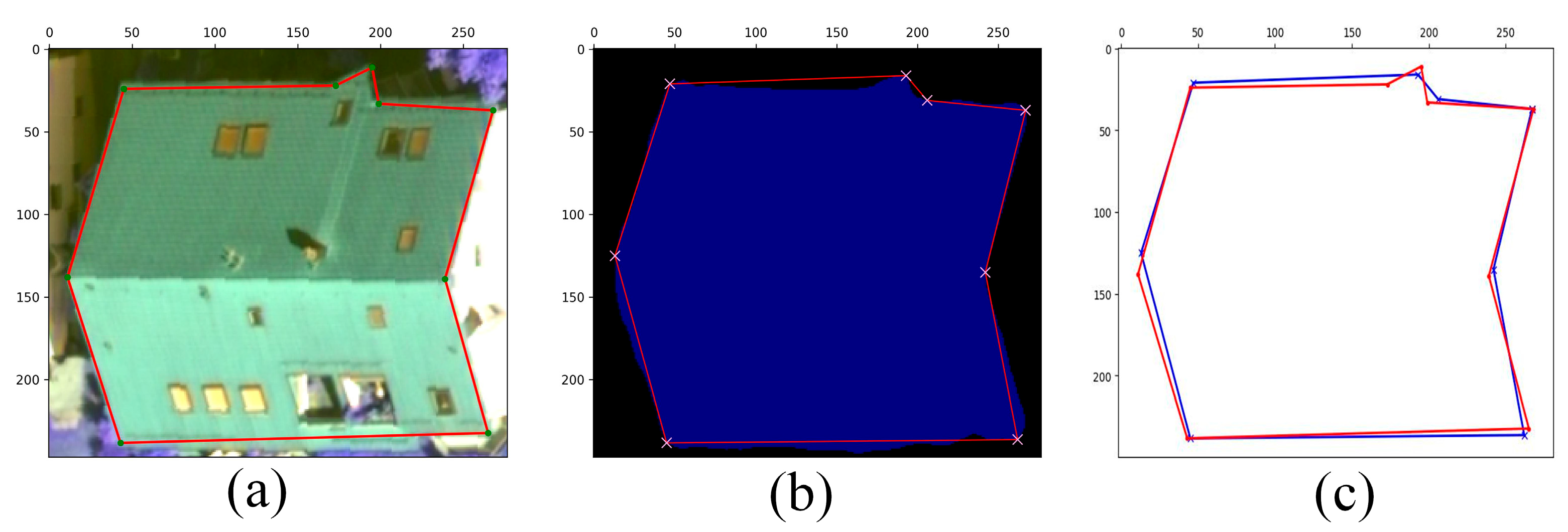
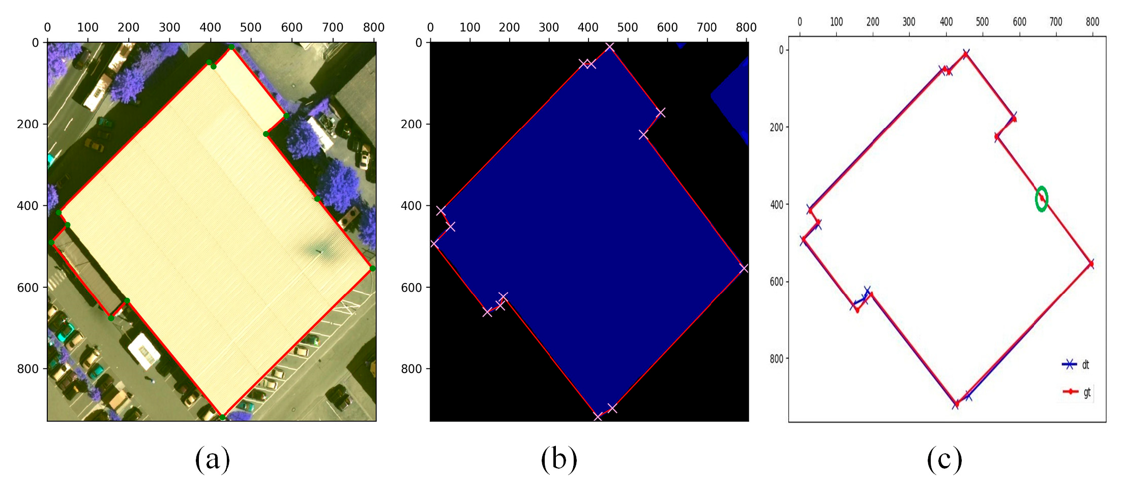
• Regularization: The vector contour is regularized. For example, we used the Douglas–Peucker (DP) [40] algorithm to obtain the inflection points of the extracted contours. Inflection points of the reference contour were obtained using manual annotations.
• Inflection point matching: We used the dynamic programming [41] inflection point matching algorithm to obtain matched pairs of inflection points. The inflection point matching problem was simplified to extract m-ordered inflection points $p_i(i=1,2,\cdots ,m)$ of the contour A. Next, A was divided into m segments. The reference contour B had q inflection points $q_j(j=1,2,\cdots ,n)$. Thereafter, B was divided into n segments. The inflection point matching of two contours was the multivalued mapping from inflection point set $a_i$ of A to inflection point set $b_i$ of B of $i:j\to \left\{i(j)\right\},$ where $i=1,2,\cdots ,m$, $i(j)=1,2,\cdots n$. There were three cases of inflection point matching of two polygon contours: one-to-one, one-to-many, and many-to-one. All inflection points are required to participate in matching; therefore, they must be surjective, meaning that the inflection point matching of the two contours is transformed into a target optimization problem.

As shown in Figure 6b, contour S and reference contour T were extracted for inflection point matching, and the best matching route is shown via the red curve in Figure 6a. The optimal match of the two contour inflection points can be determined by the line from the bottom row in the dynamic programming table. The path to the top row passes through the smallest sum of the grid values. The path can be extended horizontally or vertically, indicating a one-to-many or many-to-one path. Multiple values in the same row indicate that the extracted contour S had one inflection point corresponding to many inflection points of the reference contour T; multiple values in the same column indicate that the extracted contour S had multiple inflection points corresponding to one inflection point of the reference contour T. In Figure 6b, the inflection points that match contour S and reference contour T were extracted, and the best matching route is indicated by the red curve in Figure 6a. S and T had five inflection points each, matching the six inflection point pairs.

2.2. Mean Inflection Point Distance

The number of inflection points of the target contour extracted by the intelligent method and the reference contour may not be the same in the accuracy evaluation; the inflection points of the extracted contour and reference contour are S and T, respectively. The inflection point matching algorithm was used to match the two contour inflection points, and $s_i\to t_j$ generated k inflection point pairs. As shown in Figure 5b, the extracted contour S and reference contour T each have five inflection points, and matching produces six inflection point pairs. The distance $d_k=\Vert s_i,t_j\Vert$ matches the inflection point. The MPD_EP (mean inflection point distance of the indistinguishable edge inflection points) is calculated as follows:

$$\mathrm{MPD}\_\mathrm{EP}=\frac{{\displaystyle \sum d_k}}{k}$$

(7)

The matching inflection points of a few building contours are distant, but proximate to the matching edge. These inflection points are called edge inflection points, and the rest are called vertex inflection points (as shown in Figure 7). The inflection point of the extracted contour is far from the corresponding inflection point of the reference contour, and the distance to the corresponding edge is minuscule. Therefore, the inflection point is an edge inflection point. If it is an edge inflection point, calculating the inflection point distance with the matching inflection point cannot truly reflect the mapping accuracy; therefore, the matching inflection point of the edge inflection point is the base of its corresponding edge. There are three conditions to determine the inflection point:

(1)

The inflection point must be 1-to-n or n-to-1. If it is 1-to-1, there is no edge inflection point;

(2)

The base from the inflection point to the corresponding side is on the corresponding side;

(3)

The distance from the inflection point to the matching inflection point satisfies the following formula:

$$d(s_i,t_j)>\alpha \ast MPD,$$

(8)

where $d(s_i,t_j)$ is the distance to the corresponding inflection point and $\alpha$ is the judgment coefficient, such as 2–5.

If the distance between the inflection point and the corresponding edge meets the conditions, select any of the following formulas according to different actual conditions:

$$\{\begin{array}{l}\min (d(s_i,t_j{t}_{j+1}|t_{j-1}{t}_j))<m|\\ \min (d(s_i,t_j{t}_{j+1}|t_{j-1}{t}_j))<\beta \ast MPD\end{array},$$

(9)

where $d(s_i,t_j{t}_{j+1}|t_{j-1}{t}_j)$ is the distance between the contour inflection point and the two edges containing the corresponding inflection point; m is the number of specified pixels, such as, for example, 5–10; $\beta$ is the judgment coefficient, such as, for example, 0.5–2; and $\lambda$ is the judgment coefficient, which can be 0.5–2.

The MPD can be calculated by the following formula:

$$MPD=\{\begin{array}{l}\frac{{\displaystyle \sum _{i=1}^{k-b}d(s_i,t_j)}+{\displaystyle \sum _{i=1}^b\min (d(s_i,t_j{t}_{j+1}|t_{j-1}{t}_j))}}{n+b},m\ge n\\ \frac{{\displaystyle \sum _{i=1}^{k-b}d(s_i,t_j)}+{\displaystyle \sum _{i=1}^b\min (d(s_i,t_j{t}_{j+1}|t_{j-1}{t}_j))}}{m+b},m<n\end{array},$$

(10)

where k is the number of matching pairs of inflection points, b is the number of edge inflection points, and m and n are the numbers of inflection points of the extracted contour and reference contour, respectively.

3. Experiment and Analysis

3.1. Experimental Setting

3.1.1. Experimental Hardware and Software Environment

The network model was built using PyTorch 1.6, Python 3.7, and CUDA 10.0. The training and testing of the experiment were conducted on an Ubuntu 16.04 server with an Intel(R) Xeon(R) CPU E5-2650 v3, 32 GB RAM, and an Nvidia RTX 2080 GPU*2. We used the Adam optimizer with 0.9 momenta. The initial learning rate was 0.001, the batch size in the training phase was fixed at 2, and the image cutoff was 1792 × 1792. The network was trained for 50 epochs. Three deep learning methods were adopted in this study: PointRend [42], Swin Transformer [43], and Mask R-CNN [44]. All models used the MMDetection deep learning framework.

3.1.2. Description of Experimental Data

We used the International Society for Photogrammetry and Remote Sensing (ISPRS) benchmark of Vaihingen [45], which is an open benchmark dataset for extracting various urban targets, including buildings. The dataset contained three false-color aerial images (near-infrared, red, and green channels) with a ground resolution of 9 cm.

3.1.3. Experiment Design

We used buildings as objects of interest because of their clear boundaries and representative shapes and sizes to more objectively compare mapping accuracy results and better track the performance of the metrics [46]. To measure the reference contours corresponding to the extracted contours more rationally, we calculated metrics based on the reference contour polygons and their corresponding extracted contours, and then analyzed their performance relative to the best segmentation determined by visual inspection to examine the sensitivity of each metric to the mapping accuracy. Two different phases were designed for the experiments. In the first stage, three groups of buildings with different complexities in shape/construction (simple, fairly complex, and complex) were selected, with each group varying in size, shape, color, and roof complexity. In the second step, we evaluated the overall accuracy of 800 buildings, and the reference contours of all buildings were obtained by manual annotation.

3.2. Evaluation Metrics

Five evaluation metrics were employed for quality evaluation in this research: overall accuracy (IoU) (Equation (1)), Boundary IoU (Equation (11)), MSD (Equation (3)), MPD_EP (Equation (7)), and MPD (Equation (10)). Boundary IoU is calculated as follows:

$$Boundary IoU(G,P)=\frac{\left|(G_d\cap G)\cap (P_d\cap P)\right|}{\left|(G_d\cap G)\cup (P_d\cap P)\right|},$$

(11)

where G is the ground truth mask; P is the prediction mask; and $G_d$ and $P_d$ are sets of pixels in the boundary region of the binary mask.

3.3. Accuracy Evaluation of Buildings with Different Complexities in Shape/Construction

As shown in Figure 8, the buildings were rectangular/square, and the results extracted by the three deep learning methods were consistent with the reference contour with regard to a few edge inflection points. The experimental results are shown in Figure 8 and

Table 1. Evaluation metrics of contour extraction effects for buildings with simple structures.

Building	Method	IoU	Boundary IoU	MSD	MPD_EP	MPD
a	PointRend	97.38%	94.11%	2.83	20.66	3.15
	Swin Transformer	94.82%	87.65%	4.58	27.71	6.40
	Mask R-CNN	94.35%	87.16%	5.01	37.68	8.34
b	PointRend	95.59%	95.07%	1.89	28.75	4.41
	Swin Transformer	93.94%	92.81%	2.58	24.51	3.97
	Mask R-CNN	94.51%	93.73%	2.39	21.99	9.38
c	PointRend	94.61%	90.84%	2.68	5.39	5.39
	Swin Transformer	92.73%	86.69%	3.68	6.34	4.59
	Mask R-CNN	93.62%	88.06%	3.23	5.89	5.89

. The IoUs of three buildings extracted by the three algorithms (PointRend, Swin Transformer, and Mask R-CNN) exceeded 92%. The Boundary IoU values were all greater than 85%, while the MSD values were only larger than 5 when using the Mask R-CNN method for building a, and the quality of mask extraction was excellent. For building a, PointRend was the best among all the accuracy metrics. The MPD values for the three algorithms were 3.15, 6.40, and 8.34, and the MPD_EP values were 20.66, 27.71, and 37.68, respectively. Because of the existence of edge inflection points, the MPD_EP was more than four times the MPD, which fully demonstrates that it is essential to determine the edge inflection points. For building b, the mask metrics of PointRend had high accuracy; however, the contour accuracy of Swin Transformer was high. The MSD values of the three algorithms were 1.89, 2.58, and 2.39, and all were very small compared to the MPD values. As previously analyzed, the MSD does not consider the corresponding relations between edges when calculating distance; thus, the calculation will contain errors and cause the results to be smaller. The MPD_EP is significantly larger than the MPD when there are edge inflection points; otherwise, the MPD_EP equals the MPD.

As shown in Figure 9, the building contours were much more complex in structure, mostly irregular, and had many folded corners. The contours extracted by the three algorithms can be seen in many places to be not accurate enough; for example, the corners of building a were not extracted well, and many corners on building b were not extracted by Swin Transformer and Mask R-CNN, resulting in a line. The extraction results of building c were better in PointRend overall, but the lower right part exceeded the ground truth.

The experimental results are shown in Figure 9 and

Table 2. Evaluation metrics of contour extraction effects for buildings with more complex and irregular structures.

Building	Method	IoU	Boundary IoU	MSD	MPD_EP	MPD
a	PointRend	85.56%	73.15%	6.97	26.45	17.12
	Swin Transformer	86.33%	69.30%	8.47	39.67	19.44
	Mask R-CNN	85.61%	69.08%	8.83	47.69	25.23
b	PointRend	94.94%	91.40%	2.80	15.74	8.84
	Swin Transformer	92.30%	87.11%	4.10	31.48	11.70
	Mask R-CNN	92.38%	87.12%	3.99	64.80	12.93
c	PointRend	95.36%	90.59%	4.78	31.71	20.31
	Swin Transformer	93.81%	82.62	5.75	36.02	18.91
	Mask R-CNN	91.05%	76.47%	8.50	39.16	32.97

. For building a, the IoUs of the extracted masks by the three algorithms (PointRend, Swin Transformer, Mask R-CNN) were all lower than 90%; moreover, the Boundary IoUs were less than 75%. The accuracy of the masks extracted by the three algorithms was not high. For the accuracy evaluation of the extracted contours, the MPD_EP values were 26.45, 39.67, and 47.69; all MPD values were greater than 17; and the visual effect was consistent. Thus, all the evaluation index results show the low accuracy of the extracted contours. For building b, the IoUs of the three algorithms’ extracted masks were greater than 90%; the Boundary IoUs were greater than 87%; PointRend’s extraction results of corner and ground truth matched the best; and the MPD values were the lowest. For building c, the IoUs of the three algorithms’ extracted masks were 95.36%, 93.81%, and 91.05%; the Boundary IoUs were 90.59%, 82.62, and 76.47%; and the MPD values were 20.31, 18.91, and 32.97. Because there was a protruding part in the lower right corner of the contours extracted by PointRend, the MPD values of PointRend were larger than those of Swin Transformer.

The structures of the buildings presented in Figure 10 were much more complex, dense, and mostly irregular; thus, significant and clear errors were observed in many places in the contours extracted by the three algorithms (Figure 10). The corners of building a were not extracted well, and the building details were not extracted. For building b, Swin Transformer and PointRend had multiple mentions of the parts. For building c, all three algorithms extracted the adjacent building next to the main point of interest, and the reference contour had very large errors. The experimental results are shown in Figure 10 and

Table 3. Evaluation metrics of contour extraction effects for buildings with much more complex and denser structures.

Building	Method	IoU	Boundary IoU	MSD	MPD_EP	MPD
a	PointRend	72.07%	68.82%	16.48	95.58	47.75
	Swin Transformer	80.81%	77.80%	12.56	32.41	27.04
	Mask R-CNN	90.26%	89.92%	8.53	15.22	8.34
b	PointRend	63.86%	57.61%	18.26	34.79	30.11
	Swin Transformer	69.87%	59.40%	15.76	37.10	34.61
	Mask R-CNN	71.36%	65.33%	14.21	32.56	28.24
c	PointRend	52.52%	47.78%	53.16	109.91	109.91
	Swin Transformer	53.58%	48.60%	51.59	109.23	109.23
	Mask R-CNN	50.26%	44.48%	54.90	109.96	109.96

. For building a, the mask accuracy extracted by Mask R-CNN was high, as was the contour accuracy after regularization, which is consistent with Figure 10. For building b, the accuracy metric of the three algorithms was not high, whereas for building c, the IoUs of the three algorithms’ extracted masks were lower than 70%; the Boundary IoUs were lower than 65%; the MPD values were greater than 28; and the difference between the reference contour and the extracted contour was large. However, the Mask R-CNN results were a bit better. For building c, the performances of the three algorithms were poor, no edge inflection points existed, the MPD and MPD_EP were equal, and the error of the MPD was enormous, exceeding 109. The extraction quality of the mask was poor, and the quality of the regularized contours was equally poor.

3.4. Overall Accuracy Evaluation

In the previous subsection, we evaluated the extraction accuracy of nine representative reference buildings to analyze and compare the effectiveness and sensitivity of various metrics. However, in a real project, multiple reference polygons should be evaluated. Therefore, we selected 800 reference buildings with different shapes, colors, sizes, and structures. As listed in

Table 4. Averaged evaluation metrics of 800 buildings’ extracted contours.

Methods	IoUaverage	Boundary IoUaverage	MSDaverage	MPD_EPaverage	MPDaverage
PointRend	90.75%	89.08%	3.34	19.57	9.09
Swin Transformer	89.75%	87.79%	3.58	21.76	10.13
Mask R-CNN	89.90%	87.49%	3.93	23.49	12.05

, the three algorithms averaged the accuracy evaluation of the extracted contours; the best results were found for PointRend, the second best were found for Swin Transformer, and the worst were found for Mask R-CNN in each index. The evaluation results of the masks were consistent with the vector evaluation results proposed in this study, which demonstrates the effectiveness of the proposed index for application to buildings of different shapes and complexities. Taking PointRend as the benchmark, the differences in the IoU values of the three algorithms were less than 1%, and the differences in the Boundary IoU values were less than 2%. The two indices do not significantly differentiate the extraction results. The differences between the MPD values of PointRend and Swin Transformer, as well as PointRend and Mask R-CNN, were 1.04 and 2.06, respectively, which translates to 11.44% and 28.60%, respectively; therefore, the MPD has a higher numerical discrimination and is more sensitive to mapping accuracy. The MPD values were significantly smaller than the MPD_EP values, and greater than 10. This fully indicates that the edge inflection point plays a significant role in determining the contour accuracy, and must be distinguished.

3.5. Analysis of Experimental Results

Table 1 and Table 2 show that the PointRend algorithm outperformed the other two for extracting simple and slightly complex building outlines. Furthermore, we discovered a strong correlation between the trends revealed by IoU, BoundaryIoU, MSD, and MPD. BoundaryIoU increased as IoU increased, MSD decreased, and MPD decreased.

In Table 3, we discovered that the PointRend algorithm had a small MSD but a large MPD for building c. We discovered this through image analysis because the extracted corner points were concentrated in the lower right corner and had a large error, and the MPD was 109.91. As a result, MPD produced biased evaluation results, which is a disadvantage of this metric. The evaluation results will be even more biased if the discrete corner points are too concentrated and have a large error. Because MPD EP is much greater than MPD when there are edge corner points, distinguishing and identifying edge corner points is critical.

Finally, we extracted a large number of buildings in Table 4. Under extensive sample conditions, we discovered that IoU, BoundaryIoU, MSD, and MPD all had a strong correlation, demonstrating the effectiveness of MPD as an accuracy metric.

To summarize, all indicators performed well when building structures were simple and uncomplicated. However, when building structures were complex, all indicators had limitations, with low extraction accuracy. The advantage of MPD is that it can calculate the actual value error; however, it can have biases when discrete corner points are over-configured.

4. Discussion

4.1. Comparison with the Networks That Predict Buildings

We compared the results of PointRend [42], Swin Transformer [43], and Mask R-CNN [44] both quantitatively and qualitatively. Mask R-CNN and Swin Transformer often predicted labels on a low-resolution regular grid, e.g., 28 × 28 [47], for instance, segmentation, as a compromise between undersampling and oversampling. PointRend already achieves excellent results. Qualitatively, PointRend outputs crisp object boundaries in regions that are oversmoothed by Mask R-CNN. Quantitatively, PointRend yields significant gains on COCO and Cityscapes for both instance and semantic segmentation. For making inferences with predicted buildings, we used the adaptive subdivision technique to refine the coarse 7 × 7 prediction for class c to reach 448 × 448 in six steps. At each step, we selected and updated (at most) the N = 282 of the most uncertain points. PointRend improved the resolution by iteration to obtain a high-resolution mask (as shown in Figure 11).

Figure 12 shows the comparison results for the dataset. From top to bottom, the buildings in the first image are more regular and smaller, and all three algorithms had better extraction results. The second image has buildings with complex structures and many folded corners (shown in yellow boxes), and PointRend extracted the highest building integrity, showing sharper corners. The third image has a large building area, and the edges of the building patches extracted by Swin Transformer and Mask R-CNN show jagged edges and blurred borders. The buildings in the fourth image are very dense, and all three algorithms extracted multiple buildings as one building. To better clarify the detailed inspection, the close-ups of the selected buildings (as marked in yellow rectangles in Figure 12) from the tested images are displayed in Figure 13. From the close-up views, we can observe that PointRend was significantly better at extracting buildings with complex structures and many corners than Swin Transformer and Mask R-CNN. For buildings with a relatively large area, Swin Transformer and Mask R-CNN had obvious jagged shapes on the edges of the extraction results.

Figure 14 shows an overlay comparison of the building extraction and ground truth results obtained with different methods. The close-ups of the selected regions (as marked in red rectangles in Figure 14) in the tested images are displayed in Figure 15. For buildings with a simple structure, regular shape, and small size, the extraction results of the three algorithms are not that different; for buildings with a complex structure, such as in the second and third pictures in Figure 15, the extraction results of PointRend are significantly better than those of Swin Transformer and Mask R-CNN. The buildings in the fourth image are too dense, and all three algorithms extracted multiple buildings as one, showing a similar performance.

Based on the above analysis, we can conclude that the improvement in the performance of PointRend lies in the identification of multiscale buildings, especially large-scale and structurally complex buildings, as well as the more accurate positioning of building boundaries.

4.2. More Experiments with Different IoU and MPD Thresholds

In the instance segmentation task, the standard MS COCO metric [22] was used to evaluate the task, which included the mean average precision (AP) of the joint of multiple IoU values. The IoU was given by the following equation:

$$IoU=\frac{area(dt\cap gt)}{area(dt\cup gt)},$$

(12)

where dt and gt denote the predicted mask and the corresponding ground truth, respectively. TP and FP can be determined based on different thresholds. For example, IoU and MPD were used as thresholds. In this paper, we chose MPD thresholds of 3, 7, and 10.

$$P=\frac{TP}{TP+FP},$$

(13)

where TP is the count of true predictions for the buildings and FP is the count of false predictions for the buildings.

Specifically, AP was calculated in steps of 0.05 at 10 IoU overlap thresholds (0.50 to 0.95) [20]. [email protected]: 0.95 was calculated according to Equation (14).

$$A{P}_{@0.5:0.95}=\frac{A{P}_{0.5}+A{P}_{0.55}+\dots +A{P}_{0.9}+A{P}_{0.95}}{10},$$

(14)

The IoU was used to measure how much our predicted contour overlapped with the ground truth. In this section, because different IoU thresholds produce different levels of accuracy, multiple IoU values and MPD values were used to observe the performance of different approaches. The best results are shown in bold in

Table 5. Comparison results with different thresholds and methods.

Methods	AP[email protected]:0.9	AP[email protected]	AP[email protected]	MSD	APMPD@3	APMPD@7	APMPD@10
PointRend	0.584	0.808	0.660	3.34	0.328	0.500	0.747
Swin Transformer	0.625	0.874	0.709	3.58	0.277	0.405	0.642
Mask R-CNN	0.598	0.848	0.672	3.93	0.011	0.300	0.549

. Taking IoU as the threshold, Swin Transformer had the best performance, and the [email protected]:0.95 of the Swin Transformer exceeded that of PointRend and Mask R-CNN, which were 0.041 and 0.027, respectively. At IoUs of 0.5 and 0.75, Swin Transformer’s AP always achieved the best results, while PointRend’s results were the worst. PointRend performed best when the MPD was used as a threshold. When the MPD (unit: pixel) was 3, AP@3 exceeded 0.051 and 0.217 for Swin Transformer and Mask R-CNN, respectively, and was much larger than that of Mask R-CNN. PointRend’s AP obtained the best results, with MPDs of 7 and 10. When IoU was the threshold, Swin Transformer had the best performance, whereas when MPD was the threshold, PointRend performed the best, which is consistent with the MSD values and visual results. PointRend enhanced the image edge through iteration, and thus its boundary accuracy was the highest. Therefore, what kind of evaluation should we take? Taking mapping as an example, firstly, the mask extracted by deep learning methods was vectorized and regularized. More attention was paid to the accuracy of the vector boundary, and the mean square error was controlled according to the different scale requirements. The experimental results showed that the metrics proposed in this paper are sensitive to the mapping accuracy, consistent with the MSD value, and can calculate an accurate error value, which is highly consistent with the visual effect. The related research in this paper provides a good reference for carrying out the evaluation of the accuracy of remote sensing artificial intelligence automatic mapping.

4.3. Accuracy Analysis of HD Metrics

Table 6. Evaluation Results of the Building Counter Accuracy Using HD Metric (Unit: Pixels).

Methods	Counts of Buildings	Maximum Error	Average Error	Mean Square Error
Mask R-CNN	1721	410.83	21.89	24.21
SwinTransformer	1873	412.95	19.87	22.86
PointRend	1798	441.23	26.84	38.88

Note: A lower HD value indicates higher accuracy.

shows the results of an evaluation of the HD accuracy of building contours extracted by three algorithms: Mask R-CNN, Swin Transformer, and PointRend. The error values of all three algorithms exceeded the MPD index. Figure 16 shows that the error is mostly distributed within 80 pixels, but it is unevenly distributed. PointRend extracted the most counters for errors between 1 and 7 pixels, which is consistent with the MPD index. Swin Transformer extracted the most counters from errors ranging from 7 to 15 pixels. This contradicts the MPD index results, and is inconsistent with the visual results.

During the calculation process, the HD index considered two curves as two-point sets, ignoring the geometric relationships of points on the same curve, and only calculated the distance between one pair of points on the two curves. As a result, the HD index was sensitive to unusual data points such as noise and outliers, which can cause deviation in distance calculation results, leading to larger errors. To summarize, while the HD index could effectively measure the similarity of two point sets in certain situations, it was insensitive to contour complexity and global distance. It could not accurately assess the precision of contour extraction.

4.4. Accuracy Analysis of MPD Metrics

Table 7. Evaluation Results of Building Counter Accuracy Using MPD Metric (Unit: Pixels).

Methods	Counts of Buildings	Maximum Error	Average Error	Mean Square Error
Mask R-CNN	1721	287.321	11.87	17.02
SwinTransformer	1873	152.73	10.14	8.45
PointRend	1798	92.706	9.01	8.06

Note: A lower MPD value indicates higher accuracy.

displays the accuracy evaluation results of many building roof counters extracted by the Mask R-CNN, Swin Transformer, and PointRend. Mask R-CNN, Swin Transformer, and PointRend extracted 1721, 1873, and 1798 buildings out of 2619 building counters, respectively. Swin Transformer extracted the greatest number of buildings. The PointRend algorithm had the lowest mean error of the three algorithms, with an average error of 9.01 pixels. At the same time, Figure 17 shows that the errors were primarily distributed within 50 pixels, with only a few building outlines having errors greater than 50 pixels. The larger errors were caused by the fact that the building outlines were not extracted.

Figure 16 also shows that the errors of the three algorithms were concentrated within 15 pixels. When using the extracted results for mapping, the allowed error should be within 15 pixels according to the scale. Because iterative subdivision improves edge accuracy, PointRend had the highest number of extractions within seven pixels of error, consistent with visual effects. The indication shows that: (1) In most cases, the extraction results of the PointRend algorithm were relatively stable, but in a few exceptional cases, the extraction results of the PointRend algorithm were poor. As a result, while PointRend did not extract the greatest number of buildings, it did extract the greatest number that met the accuracy requirements. (2) The proposed method could calculate the mapping accuracy of all tested buildings effectively (by comparing the AI-extracted building roof counters with their corresponding reference counters and using the mapping accuracy evaluation method proposed in this paper to calculate the accurate mapping accuracy of each tested building). As a result of the proposed mapping accuracy evaluation method’s stability and high reliability, we demonstrated its capability.

5. Conclusions

With the rapid development of artificial intelligence, automatic mapping has become a possibility. In this study, we proposed an inflection point matching algorithm for vector polygons to match the inflection points of extracted building contours and reference contours. The definition and judgment conditions of edge inflection points were given. Aiming to address the problems that exist in the accuracy evaluation methods based on the IoU, we designed the mean inflection point distance (MPD), which can automatically calculate any two polygon contours (many-to-one and one-to-many inflection points between the extracted contour and the reference contour, with the extracted contour having more inflection points and more edges). The IoU could only calculate the percentage, not the exact error value, but the MPD can calculate the exact error value. The MPD value can be used to determine the scale suitable for mapping. Our experiments show that the MPD is more sensitive to the boundary accuracy than IoU and Boundary IoU, has a higher differentiation, and can obtain an accurate error value. The MPD has a better reference value for the accuracy requirements of mapping according to different scales. The relevant research in this paper provides a good reference for carrying out this accuracy evaluation method of artificial intelligence automated mapping. Our evaluation metrics begin with the regularization of the extracted contours, which affects the accuracy of the vector contours. As our next step, we will study the contour regularization technique to reduce the error impact of regularization.

References

1. Moser, G.; Serpico, S.B.; Benediktsson, J.A. Land-Cover Mapping by Markov Modeling of Spatial–Contextual Information in Very-High-Resolution Remote Sensing Images. Proc. IEEE 2013, 101, 631–651. [Google Scholar] [CrossRef]
2. Friedl, M.A.; McIver, D.K.; Hodges, J.C.F.; Zhang, X.Y.; Muchoney, D.; Strahler, A.H.; Woodcock, C.E.; Gopal, S.; Schneider, A.; Cooper, A.; et al. Global Land Cover Mapping from MODIS: Algorithms and Early Results. Remote Sens. Environ. 2002, 83, 287–302. [Google Scholar] [CrossRef]
3. Maus, V.; Camara, G.; Cartaxo, R.; Sanchez, A.; Ramos, F.M.; de Queiroz, G.R. A Time-Weighted Dynamic Time Warping Method for Land-Use and Land-Cover Mapping. IEEE J. Sel. Top. Appl. Earth Obs. Remote Sens. 2016, 9, 3729–3739. [Google Scholar] [CrossRef]
4. Longbotham, N.; Chaapel, C.; Bleiler, L.; Padwick, C.; Emery, W.J.; Pacifici, F. Very High Resolution Multiangle Urban Classification Analysis. IEEE Trans. Geosci. Remote Sens. 2012, 50, 1155–1170. [Google Scholar] [CrossRef]
5. Li, X.; Xu, F.; Xia, R.; Li, T.; Chen, Z.; Wang, X.; Xu, Z.; Lyu, X. Encoding Contextual Information by Interlacing Transformer and Convolution for Remote Sensing Imagery Semantic Segmentation. Remote Sens. 2022, 14, 4065. [Google Scholar] [CrossRef]
6. Fritsch, J.; Kuhnl, T.; Geiger, A. A New Performance Measure and Evaluation Benchmark for Road Detection Algorithms. In Proceedings of the 16th International IEEE Conference on Intelligent Transportation Systems (ITSC 2013), The Hague, The Netherlands, 6–9 October 2013; pp. 1693–1700. [Google Scholar]
7. Zhang, H.; Liao, Y.; Yang, H.; Yang, G.; Zhang, L. A Local–Global Dual-Stream Network for Building Extraction from Very-High-Resolution Remote Sensing Images. IEEE Trans. Neural Netw. Learn. Syst. 2022, 33, 1269–1283. [Google Scholar] [CrossRef]
8. Cheng, G.; Wang, Y.; Xu, S.; Wang, H.; Xiang, S.; Pan, C. Automatic Road Detection and Centerline Extraction via Cascaded End-to-End Convolutional Neural Network. IEEE Trans. Geosci. Remote Sens. 2017, 55, 3322–3337. [Google Scholar] [CrossRef]
9. Li, W.; He, C.; Fang, J.; Zheng, J.; Fu, H.; Yu, L. Semantic Segmentation-Based Building Footprint Extraction Using Very High-Resolution Satellite Images and Multi-Source GIS Data. Remote Sens. 2019, 11, 403. [Google Scholar] [CrossRef] [Green Version]
10. Long, J.; Shelhamer, E.; Darrell, T. Fully Convolutional Networks for Semantic Segmentation. In Proceedings of the 2015 IEEE Conference on Computer Vision and Pattern Recognition (CVPR), Boston, MA, USA, 7–12 June 2015; pp. 3431–3440. [Google Scholar]
11. Badrinarayanan, V.; Kendall, A.; Cipolla, R. SegNet: A Deep Convolutional Encoder-Decoder Architecture for Image Segmentation. IEEE Trans. Pattern Anal. Mach. Intell. 2017, 39, 2481–2495. [Google Scholar] [CrossRef]
12. Ronneberger, O.; Fischer, P.; Brox, T. U-Net: Convolutional Networks for Biomedical Image Segmentation. In Medical Image Computing and Computer-Assisted Intervention—MICCAI 2015; Navab, N., Hornegger, J., Wells, W.M., Frangi, A.F., Eds.; Lecture Notes in Computer Science; Springer International Publishing: Cham, Switzerland, 2015; Volume 9351, pp. 234–241. ISBN 978-3-319-24573-7. [Google Scholar]
13. Zhou, Z.; Rahman Siddiquee, M.M.; Tajbakhsh, N.; Liang, J. UNet++: A Nested U-Net Architecture for Medical Image Segmentation. In Deep Learning in Medical Image Analysis and Multimodal Learning for Clinical Decision Support; Stoyanov, D., Taylor, Z., Carneiro, G., Syeda-Mahmood, T., Martel, A., Maier-Hein, L., Tavares, J.M.R.S., Bradley, A., Papa, J.P., Belagiannis, V., et al., Eds.; Lecture Notes in Computer Science; Springer International Publishing: Cham, Switzerland, 2018; Volume 11045, pp. 3–11. ISBN 978-3-030-00888-8. [Google Scholar]
14. Chen, L.-C.; Papandreou, G.; Kokkinos, I.; Murphy, K.; Yuille, A.L. DeepLab: Semantic Image Segmentation with Deep Convolutional Nets, Atrous Convolution, and Fully Connected CRFs. IEEE Trans. Pattern Anal. Mach. Intell. 2018, 40, 834–848. [Google Scholar] [CrossRef] [Green Version]
15. Dai, J.; He, K.; Sun, J. Instance-Aware Semantic Segmentation via Multi-Task Network Cascades. In Proceedings of the 2016 IEEE Conference on Computer Vision and Pattern Recognition (CVPR), Las Vegas, NV, USA, 27–30 June 2016; pp. 3150–3158. [Google Scholar]
16. Luo, M.; Ji, S.; Wei, S. A Diverse Large-Scale Building Dataset and a Novel Plug-and-Play Domain Generalization Method for Building Extraction. arXiv 2022, arXiv:2208.10004. [Google Scholar]
17. Ji, S.; Wei, S.; Lu, M. Fully Convolutional Networks for Multisource Building Extraction from an Open Aerial and Satellite Imagery Data Set. IEEE Trans. Geosci. Remote Sens. 2019, 57, 574–586. [Google Scholar] [CrossRef]
18. Zhu, Q.; Liao, C.; Hu, H.; Mei, X.; Li, H. MAP-Net: Multiple Attending Path Neural Network for Building Footprint Extraction From Remote Sensed Imagery. IEEE Trans. Geosci. Remote Sens. 2021, 59, 6169–6181. [Google Scholar] [CrossRef]
19. Wang, L.; Fang, S.; Meng, X.; Li, R. Building Extraction with Vision Transformer. IEEE Trans. Geosci. Remote Sens. 2022, 60, 1–11. [Google Scholar] [CrossRef]
20. Jin, Y.; Xu, W.; Zhang, C.; Luo, X.; Jia, H. Boundary-Aware Refined Network for Automatic Building Extraction in Very High-Resolution Urban Aerial Images. Remote Sens. 2021, 13, 692. [Google Scholar] [CrossRef]
21. Fang, F.; Wu, K.; Liu, Y.; Li, S.; Wan, B.; Chen, Y.; Zheng, D. A Coarse-to-Fine Contour Optimization Network for Extracting Building Instances from High-Resolution Remote Sensing Imagery. Remote Sens. 2021, 13, 3814. [Google Scholar] [CrossRef]
22. Lin, T.Y.; Maire, M.; Belongie, S.; Hays, J.; Zitnick, C.L. Microsoft COCO: Common Objects in Context; Springer International Publishing: Berlin/Heidelberg, Germany, 2014. [Google Scholar]
23. Rezatofighi, H.; Tsoi, N.; Gwak, J.Y.; Sadeghian, A.; Savarese, S. Generalized Intersection Over Union: A Metric and a Loss for Bounding Box Regression. In Proceedings of the 2019 IEEE/CVF Conference on Computer Vision and Pattern Recognition (CVPR), Long Beach, CA, USA, 15–20 June 2019. [Google Scholar]
24. Zheng, Z.; Wang, P.; Liu, W.; Li, J.; Ye, R.; Ren, D. Distance-IoU Loss: Faster and Better Learning for Bounding Box Regression. Proc. AAAI Conf. Artif. Intell. 2020, 34, 12993–13000. [Google Scholar] [CrossRef]
25. Cheng, B.; Girshick, R.; Dollár, P.; Berg, A.C.; Kirillov, A. Boundary IoU: Improving Object-Centric Image Segmentation Evaluation. In Proceedings of the IEEE/CVF Conference on Computer Vision and Pattern Recognition, Nashville, TN, USA, 20–25 June 2021. [Google Scholar]
26. Everingham, M.; Van Gool, L.; Williams, C.K.; Winn, J.; Zisserman, A. The PASCAL Visual Object Classes (VOC) Challenge. Int. J. Comput. Vis. 2010, 88, 303–338. [Google Scholar] [CrossRef] [Green Version]
27. Heimann, T.; Van Ginneken, B.; Styner, M.A.; Arzhaeva, Y.; Aurich, V.; Bauer, C.; Beck, A.; Becker, C.; Beichel, R.; Bekes, G.; et al. Comparison and Evaluation of Methods for Liver Segmentation From CT Datasets. IEEE Trans. Med. Imaging 2009, 28, 1251–1265. [Google Scholar] [CrossRef] [PubMed]
28. Zhu, Y.; Huang, B.; Gao, J.; Huang, E.; Chen, H. Adaptive Polygon Generation Algorithm for Automatic Building Extraction. IEEE Trans. Geosci. Remote Sens. 2022, 60, 1–14. [Google Scholar] [CrossRef]
29. Wu, Y.; Xu, L.; Chen, Y.; Wong, A.; Clausi, D.A. TAL: Topography-Aware Multi-Resolution Fusion Learning for Enhanced Building Footprint Extraction. IEEE Geosci. Remote Sens. Lett. 2022, 19, 1–5. [Google Scholar] [CrossRef]
30. Kristan, M.; Leonardis, A.; Matas, J.; Felsberg, M.; Pflugfelder, R.; Čehovin, L.; Vojír, T.; Häger, G.; Lukežič, A.; Fernández, G.; et al. The Visual Object Tracking VOT2016 Challenge Results. In Lecture Notes in Computer Science, Proceedings of the Computer Vision—ECCV 2016 Workshops, Amsterdam, The Netherlands, 8–16 October 2016; Hua, G., Jégou, H., Eds.; Springer International Publishing: Cham, Switzerland, 2016; pp. 777–823. [Google Scholar]
31. Baltsavias, E.P. Object Extraction and Revision by Image Analysis Using Existing Geodata and Knowledge: Current Status and Steps towards Operational Systems. ISPRS J. Photogramm. Remote Sens. 2004, 58, 129–151. [Google Scholar] [CrossRef]
32. Lowe, D.G. Object Recognition from Local Scale-Invariant Features. In Proceedings of the Seventh IEEE International Conference on Computer Vision, Kerkyra, Greece, 20–27 September 1999; Volume 2, pp. 1150–1157. [Google Scholar]
33. Redmon, J.; Divvala, S.; Girshick, R.; Farhadi, A. You Only Look Once: Unified, Real-Time Object Detection. In Proceedings of the 2016 IEEE Conference on Computer Vision and Pattern Recognition (CVPR), Las Vegas, NV, USA, 27–30 June 2016; pp. 779–788. [Google Scholar]
34. Di, Y.; Shao, Y.; Chen, L.K. Real-Time Wave Mitigation for Water-Air OWC Systems Via Beam Tracking. IEEE Photonics Technol. Lett. 2021, 34, 47–50. [Google Scholar] [CrossRef]
35. Leal-Taixé, L.; Milan, A.; Reid, I.; Roth, S.; Schindler, K. MOTChallenge 2015: Towards a Benchmark for Multi-Target Tracking. arXiv 2015, arXiv:1504.01942. [Google Scholar]
36. Automated Segmentation of Colorectal Tumor in 3D MRI Using 3D Multiscale Densely Connected Convolutional Neural Network. Available online: https://www.hindawi.com/journals/jhe/2019/1075434/ (accessed on 20 February 2023).
37. Hung, W.-L.; Yang, M.-S. Similarity Measures of Intuitionistic Fuzzy Sets Based on Hausdorff Distance. Pattern Recognit. Lett. 2004, 25, 1603–1611. [Google Scholar] [CrossRef]
38. Rote, G. Computing the Minimum Hausdorff Distance between Two Point Sets on a Line under Translation. Inf. Process. Lett. 1991, 38, 123–127. [Google Scholar] [CrossRef]
39. Suzuki, S.; Be, K. Topological Structural Analysis of Digitized Binary Images by Border Following. Comput. Vis. Graph. Image Process. 1985, 30, 32–46. [Google Scholar] [CrossRef]
40. Douglas, D.H.; Peucker, T.K. Algorithms for the Reduction of the Number of Points Required to Represent a Digitized Line or Its Caricature. In Classics in Cartography; Dodge, M., Ed.; Wiley: Hoboken, NJ, USA, 2011; pp. 15–28. ISBN 978-0-470-68174-9. [Google Scholar]
41. Petrakis, E.; Diplaros, A.; Milios, E. Matching and Retrieval of Distorted and Occluded Shapes Using Dynamic Programming. Pattern Anal. Mach. Intell. IEEE Trans. 2002, 24, 1501–1516. [Google Scholar] [CrossRef]
42. Kirillov, A.; Wu, Y.; He, K.; Girshick, R. PointRend: Image Segmentation as Rendering. In Proceedings of the 2020 IEEE/CVF Conference on Computer Vision and Pattern Recognition (CVPR), Seattle, WA, USA, 13–19 June 2020; pp. 9796–9805. [Google Scholar]
43. Liu, Z.; Lin, Y.; Cao, Y.; Hu, H.; Wei, Y.; Zhang, Z.; Lin, S.; Guo, B. Swin Transformer: Hierarchical Vision Transformer Using Shifted Windows. In Proceedings of the 2021 IEEE/CVF International Conference on Computer Vision (ICCV), Montreal, QC, Canada, 11–17 October 2021; pp. 9992–10002. [Google Scholar]
44. He, K.; Gkioxari, G.; Dollar, P.; Girshick, R. Mask R-CNN. In Proceedings of the 2017 IEEE International Conference on Computer Vision (ICCV), Venice, Italy, 22–29 October 2017; pp. 2980–2988. [Google Scholar]
45. Rottensteiner, F.; Sohn, G.; Gerke, M.; Wegner, J.D.; Breitkopf, U.; Jung, J. Results of the ISPRS Benchmark on Urban Object Detection and 3D Building Reconstruction. ISPRS J. Photogramm. Remote Sens. 2014, 93, 256–271. [Google Scholar] [CrossRef]
46. Jozdani, S.; Chen, D. On the Versatility of Popular and Recently Proposed Supervised Evaluation Metrics for Segmentation Quality of Remotely Sensed Images: An Experimental Case Study of Building Extraction. ISPRS J. Photogramm. Remote Sens. 2020, 160, 275–290. [Google Scholar] [CrossRef]
47. He, K.; Zhang, X.; Ren, S.; Sun, J. Deep Residual Learning for Image Recognition. In Proceedings of the 2016 IEEE Conference on Computer Vision and Pattern Recognition (CVPR), Las Vegas, NV, USA, 27–30 June 2016; pp. 770–778. [Google Scholar]
Figure 1. Vector image accuracy evaluation: (a) original image and reference contours; (b) deep learning extracted mask and regularized contours; (c) the two contours to be evaluated.
Remotesensing 15 01848 g001
Figure 2. There are several scenarios where IoU values are equal. The red boxes in (ad) represent the same reference contour with equal IoU values. The blue boxes indicate the contours to be evaluated, where (ac) are the same but have different positions. BoundaryIoU represents the intersection over a union of the extracted contour and the reference contour within a particular buffer zone of distance d. Here, we take d as the minimum value. The overlap between the two contours is represented by red and blue dashed lines. In (c), there are only two overlapping points so the BoundaryIoU value is 0.
Remotesensing 15 01848 g002
Figure 3. The MSD of (a,b) are equal, but the contour of (b) is significantly better. The shortest distances between the points on S3S4 (yellow line) and the reference contour T are the distances between the points on edge S3S4 and point (S3 or S4), respectively, which are both on edge S3S4; thus, M S D ( S 1 , T ) = M S D ( S 2 , T ) . An error is added when calculating the average distance between two contours. This is because, when calculating the distance between two contours, the closest distance from the point to the reference contour is used to approximate the distance from the point to the corresponding edge, ignoring the correspondence between the contours and the edges.
Remotesensing 15 01848 g003
Figure 4. Two contours, where red is Y and blue is X. dXY is the maximum distance from X to Y. dYX is the maximum distance from Y to X, because d X Y < d Y X . Therefore, H ( X , Y ) = d Y X .
Remotesensing 15 01848 g004
Figure 5. Overall flowchart of MPD.
Remotesensing 15 01848 g005
Figure 6. Inflection point matching. (a) This is a DP table, and a path in the table can be represented as follows: starting from the bottom row with a certain direction (left or right), moving to the grid with the minimum value in the DP table one grid at a time, and ending at the vertex row. The red line in (a) represents the matching result of the inflection points of two contours in (b). (b) The inflection points matching contour S and reference contour T are extracted, and the best matching route is shown in the red curve in (a). S and T each has five inflection points, matching six inflection point pairs.
Remotesensing 15 01848 g006
Figure 7. Contours with edge inflection points. (a) Original image and reference contour; (b) extracted mask and regularized contours; (c) two overlapping contours. The inflection point in the green circle is very close to the edge, and the corresponding inflection point is a large distance away; thus, the point is an edge inflection point.
Remotesensing 15 01848 g007
Figure 8. Contour extractions for buildings with simple structures. (ae) are respectively the original image, ground truth, PointRend, Swin Transformer, and Mask R-CNN. The red line represents the ground truth, the blue line represents the extracted contour, and X denotes the edge inflection points of the vector contour.
Remotesensing 15 01848 g008
Figure 9. Contour extractions for buildings with more complex and irregular structures. (ae) are respectively the original image, ground truth, PointRend, Swin Transformer, and Mask R-CNN. The red line represents the ground truth, the blue line represents the extracted contour, and X denotes the edge inflection points of the vector contour.
Remotesensing 15 01848 g009
Figure 10. Contour extractions for buildings with complex structures. (ae) are respectively the original image, ground truth, PointRend, Swin Transformer, and Mask R-CNN. The red line represents the ground truth, the blue line represents the extracted contour, and X denotes the edge inflection points of the vector contour.
Remotesensing 15 01848 g010
Figure 11. Example of one adaptive subdivision step. The red dots are the points that need to be inferred for each iteration.
Remotesensing 15 01848 g011
Figure 12. Examples of building extraction results obtained by different methods. (a) Original image. (b) PointRend. (c) Swin Transformer. (d) Mask R-CNN. The yellow rectangles in (bd) are the selected buildings for close-up inspection, shown in Figure 13.
Remotesensing 15 01848 g012
Figure 13. Close-up view of individual building results obtained by different methods. (a) Original image. (b) Ground truth. (c) PointRend. (d) Swin Transformer. (e) Mask R-CNN.
Remotesensing 15 01848 g013
Figure 14. Examples of building extraction results obtained by different methods. (a) Original image. (b) Ground truth. (c) PointRend. (d) Swin Transformer. (e) Mask R-CNN. Note, in columns (ce), yellow, green, and red indicate true-positive, false-negative, and false-positive, respectively. The red rectangles in (a) are the selected regions for close-up inspection, shown in Figure 15.
Remotesensing 15 01848 g014
Figure 15. Close-up views of the results obtained by different methods. Images and results shown in (ae) are the subset from the selected regions marked in Figure 9a. (a) Original image. (b) Ground truth. (c) PointRend. (d) Swin Transformer. (e) Mask R-CNN.
Remotesensing 15 01848 g015
Figure 16. HD distribution histogram.
Remotesensing 15 01848 g016
Figure 17. MPD distribution histogram.
Remotesensing 15 01848 g017