Article

Multi-Resolution Population Mapping Based on a Stepwise Downscaling Approach Using Multisource Data

1
School of Geographic and Biologic Information, Nanjing University of Posts and Telecommunications, Nanjing 210023, China
2
Smart Health Big Data Analysis and Location Services Engineering Lab of Jiangsu Province, Nanjing 210023, China
3
School of Geographic Sciences, Nanjing University of Information Science and Technology, Nanjing 210044, China
*
Author to whom correspondence should be addressed.
Remote Sens. 2023, 15(7), 1947; https://doi.org/10.3390/rs15071947
Submission received: 25 January 2023 / Revised: 31 March 2023 / Accepted: 4 April 2023 / Published: 6 April 2023
(This article belongs to the Section Remote Sensing for Geospatial Science)

Abstract

:
The distribution of the population is an essential aspect of addressing social, economic, and environmental problems. Gridded population data can provide more detailed information than census data, and multisource data from remote sensing and geographic information systems have been widely used for population estimation studies. However, due to spatial heterogeneity, the population has different distribution characteristics and variation patterns at different scales, while the relationships between multiple variables also vary with scale. This article presents a stepwise downscaling approach in that the random forest regression kriging technique is used to downscale census data to multi-resolution gridded population datasets. Using Nanjing, China, as the experimental case, population distribution maps were generated at 100 m, 500 m, and 1 km spatial resolution, and compared with the other three downscaling methods and three population products. The results demonstrated the produced gridded population maps by the proposed approach have higher accuracy and more accurate details of population distribution with the smallest mean absolute error (MAE) and root mean squared error (RMSE) values of 1.590 and 2.189 ten thousand people (over 40% reduction). The artificial land and road data are the two most important indicators of population distribution for the regional random forest modeling in Nanjing. Our proposed method can be a valuable tool for population mapping and has the potential to monitor sustainable development goals.

1. Introduction

The spatial distribution of the population and its changes have been an essential topic of urban geography, economics, and urban planning research, which have received widespread attention [1,2,3]. Traditional spatial population data are mainly derived from field surveys, in the case of Chinese census data, a national household survey is conducted every 10 years and a 1% sample survey is conducted every 5 years [4]. While authoritative, systematic, and standardized, these data are often not up-to-date, and the demographic statistics cannot fully reflect the actual spatial distribution of the population. As a result, they cannot effectively reveal the spatial variability of population distribution within cities. The population spatialization provides a visual and multi-scale representation of the actual distribution of the population [5,6], which serves as a refinement and supplement to the statistical data. Understanding the spatial distribution of the population at a finer spatial scale is of great value for many applications, such as urban expansion and population migration, disaster prevention and relief operations, resource allocation, and sustainable development assessment [7,8]. Multi-resolution gridded population data are the basis for analysis at different resolutions, such as tracking United Nations Sustainable Development Goals (SDGs) using the population data of different spatial resolutions [9,10].
With the continuous development of population spatialization research, various methods have been developed to downscale the census data [11,12], and a series of gridded population products have emerged [13,14,15]. The spatialization methods can be summarized as spatial interpolation and statistical modeling [16], as well as hybrid methods. Spatial interpolation is the conversion of census data from a source unit (i.e., census unit) to a target spatial unit, including point interpolation [17] and areal interpolation [18]. Based on the assumption that the population distribution decays with distance, the point interpolation method is used to map the population distribution by interpolating the selected control points within the region, such as kernel interpolation [19]. The areal interpolation maps population distribution by multiplying the population density within different units with their corresponding areas, such as the areal weighting method and dasymetric mapping [20], which assumes a uniform or proportional distribution of population within administrative units. The areal weighting method has been applied to generate the Gridded Population of the World, a global 1 km population product [21]. Subsequently, auxiliary data were incorporated into spatial interpolation as control points [22] or a basis for the division of different population density regions [23]. However, the assumptions of spatial interpolation methods could make them prone to errors when applied in regions of heterogeneity.
Compared with spatial interpolation, the statistical modeling method can better utilize the spatial distribution information of the population in multisource data by establishing the relationship between the population and the auxiliary variables [24]. Common statistical modeling includes linear regression models (e.g., multiple linear regression [25,26], spatial regression models (e.g., geographically weighted regression (GWR) [27]), and artificial intelligence algorithms (e.g., extreme gradient boosting (XGboost), random forest and convolutional neural network [7,28]). However, linear models assume a linear relationship between the population and the auxiliary variables, making it difficult to capture the spatial heterogeneity of population distribution [29]. Although the GWR model takes spatial heterogeneity into account, sometimes invalid or meaningless predictions would occur, such as appearing in negative populations in rural areas [30]. Meanwhile, artificial intelligence algorithms are widely used in population mapping due to their strong ability to mine relationships between multiple variables [31,32]. Among them, random forest is an integrated learning method consisting of multiple decision trees less prone to overfitting, which is the most popular method used for mapping population distribution [16,33]. Worldpop releases the global gridded population maps at two spatial resolutions (100 m and 1 km) each year by employing a random forest model [34]. Moreover, the hybrid methods generally integrate different methods to improve the prediction performance by exploiting the advantages of the different methods, such as interpolation dasymetric and statistical dasymetric [35,36,37], which combine spatial interpolation and statistical modeling with dynamic mapping. For example, Roni et al. [38] proposed a population disaggregation model by incorporating GWR into a dasymetric model, which performed better than traditional dasymetric mapping.
Most population mapping studies have focused on the study of models and modeling factors, which are the two most important aspects of modeling populations [8]. The mentioned statistical modeling methods usually establish a regression model at the census unit scale [39], which is considered applicable on both the source and target scales. However, due to spatial heterogeneity being a common phenomenon in the spatial distribution of population, the relationship between the population and multiple geographical variables would change with scale [40]. In the case of scale variation, there is a mismatch between the training data and the predicted data, resulting in low accuracy of population mapping [41]. Meanwhile, dominant auxiliary variables for population density distribution also vary at different scales. On the other hand, with the increasing abundance of auxiliary data for population spatialization, the combination of multiple natural and socioeconomic factors has become a trend in population mapping [8,29], including remotely sensed data (e.g., land cover/land use, vegetation information, and night light) and geospatial data (e.g., points of interest (POIs), road and transportation). As mentioned, machine learning methods could capture the complex non-linear relationships that exist between the population and multiple geographical factors [7,42]. However, as errors in all input data are propagated cumulatively during the downscaling process, this may significantly affect the accuracy of the final prediction [40]. Considering the error propagation contribution of an auxiliary variable might be greater than its contribution to modeling, there would be little discrepancy in the performance of the model on the training and test datasets before and after the reduction in variables. Hence, it might be possible to enhance prediction accuracy by choosing optimal variables. In addition, although global and regional population products have emerged at different resolutions, differences in input data and modeling methods make these gridded population data significantly different in terms of accuracy and quality [6,43]. Fewer population products are currently available with multiple resolutions.
Hence, this paper designed a stepwise downscaling framework based on the random forest regression kriging to generate a multi-resolution gridded population. For each different spatial resolution, the random forest regression kriging model was established by selecting the corresponding optimal auxiliary variables. This strategy reduces input errors by selecting the most relevant variables and narrows the mismatch between the training and predicted data through stepwise downscaling, resulting in more accurate downscaled results. The established random forest regression kriging models of the previous coarse spatial resolution were employed in the following finer spatial resolution. The proposed stepwise downscaling approach was validated in Nanjing, China, using sixth and seventh national census data (i.e., 2010 and 2020 census data) to generate population distribution maps at 1 km, 500 m, and 100 m spatial resolution. To compare the multi-resolution population mapping of 2010 and 2020, three methods and three population products were used, including WorldPop, LandScan, and China population mapping. Furthermore, the predicted multi-resolution population data were also used to explore one of the SDGs indices to discuss their potential applications.

2. Materials and Methods

2.1. Study Area

Nanjing is the capital city of Jiangsu Province, located at 118°22′~119°14′E and 31°14′~32°37′N, in the middle of the lower reaches of the Yangtze River and southwest of Jiangsu Province, China (see Figure 1). Nanjing has a total area of 6597 km², with a main urban area of 243 km2, which is long in the north-south direction and narrow in the east-west direction. As of 2020, Nanjing has 11 districts and 9.31 million (referred to Nanjing statistics agency), including Xuanwu District, Qinhuai District, Jianye District, Gulou District, Pukou District, Qixia District, Yuhuatai District, Jiangning District, Liuhe District, Lishui District, and Gaochun District. Compared to 2010, the population has increased by 1.31 million, and the Baixia and Xiaguan districts have been abolished. It has a subtropical monsoon climate [44] and is a hilly and mountainous terrain with low hills and gentle hills. With the rapid development of regional integration in the Yangtze River Delta, Nanjing has emerged as a mega-city and a sub-center city within the Yangtze River Delta Economic Zone. Detailed population information within administrative units is crucial for the urban planning and sustainable development of Nanjing. In this paper, we define the study domain as Nanjing City, which ranks among the top 10 municipalities and provincial capitals in China in terms of regional GDP [45].

2.2. Materials and Data Processing

Based on the statistics of the district from the Nanjing statistics agency and the official websites of each district, we have collected 2010 and 2020 Nanjing census data (shown in Figure 2), including complete population data for each district, complete population data for each administrative street zone in 2010 (121 administrative streets), and population data for partial administrative street zone in 2020 (39 of 107 administrative streets until 22 February 2023). Although several street-level population data are also publicly available on other websites, this study only considers information from authoritative sources. The auxiliary geographical factors influencing the population were collected from two types of data sources: geospatial data and remote sensing data. Table 1 provides the list of datasets and sources used in this study. All auxiliary data were generated and resampled to three spatial resolutions, 1 km, 500 m, and 100 m.

2.2.1. Geospatial Data

Geospatial data includes basic geographic data and OpenStreetMap (OSM) data. Basic geospatial data were obtained from the National Geomatics Center of China and the Department of Natural Resources of Jiangsu Province, such as administrative boundaries, water area, railway, and road. The rasterized water data at 1 km, 500 m, and 100 m were used as masks for population predictions at corresponding resolutions for 2010 and 2020. The OSM contains more detailed information about the city, which helps in making population predictions. The POIs, transportation (Trans), railway (Rail) and road (Road) were extracted for the study area in 2013 and 2020. The 2013 data were used as a proxy for the 2010 data. To obtain the final railway and road data, we merged information from basic geospatial data and OSM data. The kernel density analysis was applied to POIs, transportation, railway, and road. The density layers of these four variables with various bandwidths were used to establish the random forest models by combing other remote sensing auxiliary variables. The optimal bandwidth for kernel density estimation was 2500 m in this experiment, corresponding to the highest accuracy model accuracy.

2.2.2. Remote Sensing Data

The remote sensing product utilized in this study comprises six components, including DEM, vegetation, land surface temperature (LST), night light (NL), land cover (LC), and WorldPop. We acquired the DEM data from the ASTER Global Digital Elevation Model V003 product, which has a spatial resolution of 30 m. The slope direction analysis was carried out to obtain four slope directions: shady, sunny, semi-shady, and semi-sunny slopes, denoted from Aspect1 to Aspect4 and slope analysis was carried out to obtain the percentage of areas with slopes no greater than 5°, marked as Slope5. The vegetation and LST data were obtained from the MODIS products, MOD11A1 and MOD13A2. The different vegetation indices (VIs), NDVI, EVI, and NIRv were extracted as auxiliary variables. The daily LST and 16-day vegetation indices were synthesized as annual maximums in 2010 and 2020, respectively. The NL data with a spatial resolution of 500 m was obtained from a global NPP-VIIRS-like NL product [46]. The average nighttime light index (NLave) and compounded nighttime light index (CNLI) [47] were extracted as auxiliary variables. The LC data were obtained from the GlobeLand30 product with a spatial resolution of 30 m (http://www.globallandcover.com/, accessed on 19 June 2022). Seven LC types occur in the study area, including cropland, forest, grass, wetland, water, artificial land, and bare land, denoted from LC1 to LC7, respectively. The proportion of each land cover type was employed as an auxiliary variable with different spatial resolutions. The WorldPop global population data set (https://hub.WorldPop.org/, accessed on 8 June 2022) was a widely used gridded population counts data provided by the University of Southampton at two spatial scales of 3 and 30 arc-seconds. The WorldPop data were resampled to 1 km and 100 m, and then employed to compare with the downscaled population predictions. The LandScan global population database of 30 arc-seconds (https://landscan.ornl.gov/landscan-datasets, accessed on 24 February 2023) and China Population mapping of 100 m generated by Ye et al. [48] were also employed to compare with the predicted gridded population results.
Table 1. List of datasets and sources used in this study.
DatasetsSourcesTimeSpatial ResolutionIndicatorsResampling
Census dataNanjing Government, China2010
2020
District level
Street level
//
WorldPopWorldPop
Mainland China
2010
2020
3 arc-seconds
30 arc-seconds
/1 km × 1 km
100 m × 100 m
LandScanLandScan
Mainland China
2010
2020
30 arc-seconds/1 km × 1 km
Population mappingYe et al. [48]2010100 m/100 m × 100 m
OSM dataOSM project2013
2020
VectorPOIs, Trans, Rail, RoadStreet level
1 km × 1 km
500 m × 500 m
100 m × 100 m
Basic geospatial dataNational Geomatics Center of China2021VectorWater area, Rail, Road, Partial POIs
Department of Natural Resources of Jiangsu Province2019VectorRail, Road, Boundary
DEMASTER Global Digital Elevation Model V0032010
2020
30 m RasterFour slope directions,
Slope ≤ 5°
VegetationMOD13A22010
2020
1 km RasterAnnual maximum NDVI, EVI, NIRv
LSTMOD11A12010
2020
1 km RasterAnnual maximum LST
Night lightGlobal NPP-VIIRS-like NL product2010
2020
500 m RasterNlave, CNLI
Land coverGlobeLand302010
2020
30 m RasterCropland, forest, grass, wetland, water, artificial land, bare land

2.3. Stepwise Downscaling

To address the problems of dynamic relationships at different scales in the downscaling process, this study describes a stepwise downscaling strategy for gridded population distribution mapping at multiple resolutions. Given the spatial resolution of auxiliary data on natural factors used in this study, we employed the stepwise downscaling approach to generate gridded population predictions at three resolutions. These predictions at 1 km, 500 m, and 100 m resolutions provide a more detailed representation of population distribution within administrative units. The method and the specific flowchart were presented in the following sub-sections. In this study, the methods and analyses were mainly implemented using the R software.

2.3.1. Stepwise Downscaling Model

The downscaling strategy mainly repeats three steps: (a) establish the regression model at the coarse resolution and estimate the relative importance of each variable; (b) perform the regression model with selected covariates at the finer resolution; (c) correct the simulated population. The random forest regression kriging method is used repeatedly to downscale population distribution from an administrative unit scale (administrative street zone) to multiple resolutions (1 km, 500 m, and 100 m). Random forest, as a nonparametric method, has been widely applied to classification [49] and regression, which integrates multiple tree models trained from sample data. Regression kriging is a hybrid technique that uses kriging to interpolate the residuals of regression models. The random forest regression kriging model, as a regression-kriging form improves the predictions from the random forest regression model by using kriging to interpolate the residuals of the random forest models [50].
Let Z(HCJ) and Xk(HCJ) be the population and corresponding k ancillary variables at coarse unit or pixel HCJ, and Xk(HFj) be the ancillary variables at finer pixel HFj. The random forest regression model between Z(HCJ) and Xk(HCJ) can be established and denoted as fCRF, which would also perform the predictor variable’s relative importance. Based on ensuring the performance of the regression model, the optimal variables can be selected for regression modeling to reduce the error induced by input data according to the rank of the predictor variable’s relative importance. The finer-resolution trend component of the population would be estimated by bringing selected predictor variables Xk(HFj) into the corresponding regression model fCRF. Meanwhile, through the original value and predicted value of the population, the regression residuals at coarse resolution can be obtained from their differences, which would be interpolated into finer-resolution pixels by using the ordinary kriging method. Then the predicted population Z(HFj) at finer resolution using random forest regression kriging can be expressed as:
Z ( H F j ) = f C RF ( X k ( H F j ) ) + J = 1 N λ J [ Z ( H C J )   -   f C RF ( X k ( H C J ) ) ] ,  
where λJ is the weight assigned to Jth neighboring unit or pixel for the estimated value in the kriging method.
In population mapping, the census data need to be disaggregated to the pixel scale. Hence, the population density distribution should be controlled by the census data at the administrative unit scale. Similarly, for the stepwise downscaling, finer spatial-resolution population data are obtained from the coarse spatial-resolution data. The sum of values of the covered finer pixels should be consistent with the corresponding coarse pixel. It is necessary to adjust the simulated gridded population according to the actual population at the administrative unit and coarse pixels. In this study, the census data at the district level and predicted population at coarse resolution were employed to adjust the simulated population derived from Equation (1). The corrected population at the pixel level is shown as:
Z P ( H F j ) = POP upper m = 1 N F upper Z ( H F m ) × Z ( H F j ) ,  
where Zp(HFj) represents the corrected population of pixel HFj, Z(HFj) is the corresponding predicted value of the grid HFj before correction, POPupper is the statistical population of an administrative district zone or the predicted gridded population, NFupper is the number of pixels at F resolution within the administrative district zone or the coarse pixel, and the denominator is the total predicted gridded population of the corresponding coarse zone.
The population mapping at different spatial resolutions can be obtained by reusing Equations (1) and (2). A three-step downscaling strategy was employed to generate gridded population data at 1 km, 500 m, and 100 m. First, the statistical population data of administrative street units were downscaled to a 1 km spatial resolution, which can be estimated as followed:
Z P ( H 1 km j ) = POP census m = 1 N 1 km census Z ( H 1 km m ) × [ f street RF ( X k ( H 1 km j ) ) + J = 1 N λ J [ Z ( H street J ) - f street RF ( X k ( H street J ) ) ] ] .  
Second, the above population predictions at a 1 km spatial resolution were downscaled to a 500 m spatial resolution, which can be written as:
Z P ( H 500 m j ) = POP 1 km m = 1 N 500 m 1 km Z ( H 500 m m ) × [ f 1 km RF ( X k ( H 500 m j ) ) + J = 1 N λ J [ Z ( H 1 km J ) - f 1 km RF ( X k ( H 1 km J ) ) ] ] .  
Then, the above population predictions at 500 m spatial resolution were downscaled to 100 m spatial resolution, where Zp(H100mj) is the predicted population distribution value of pixel H100mj at 100 m resolution:
Z P ( H 100 m j ) = POP 500 m m = 1 N 100 m 500 m Z ( H 100 m m ) × [ f 500 m RF ( X k ( H 100 m j ) ) + J = 1 N λ J [ Z ( H 500 m J ) - f 500 m RF ( X k ( H 500 m J ) ) ] ] .  

2.3.2. Flowchart of Multi-Resolution Population Mapping

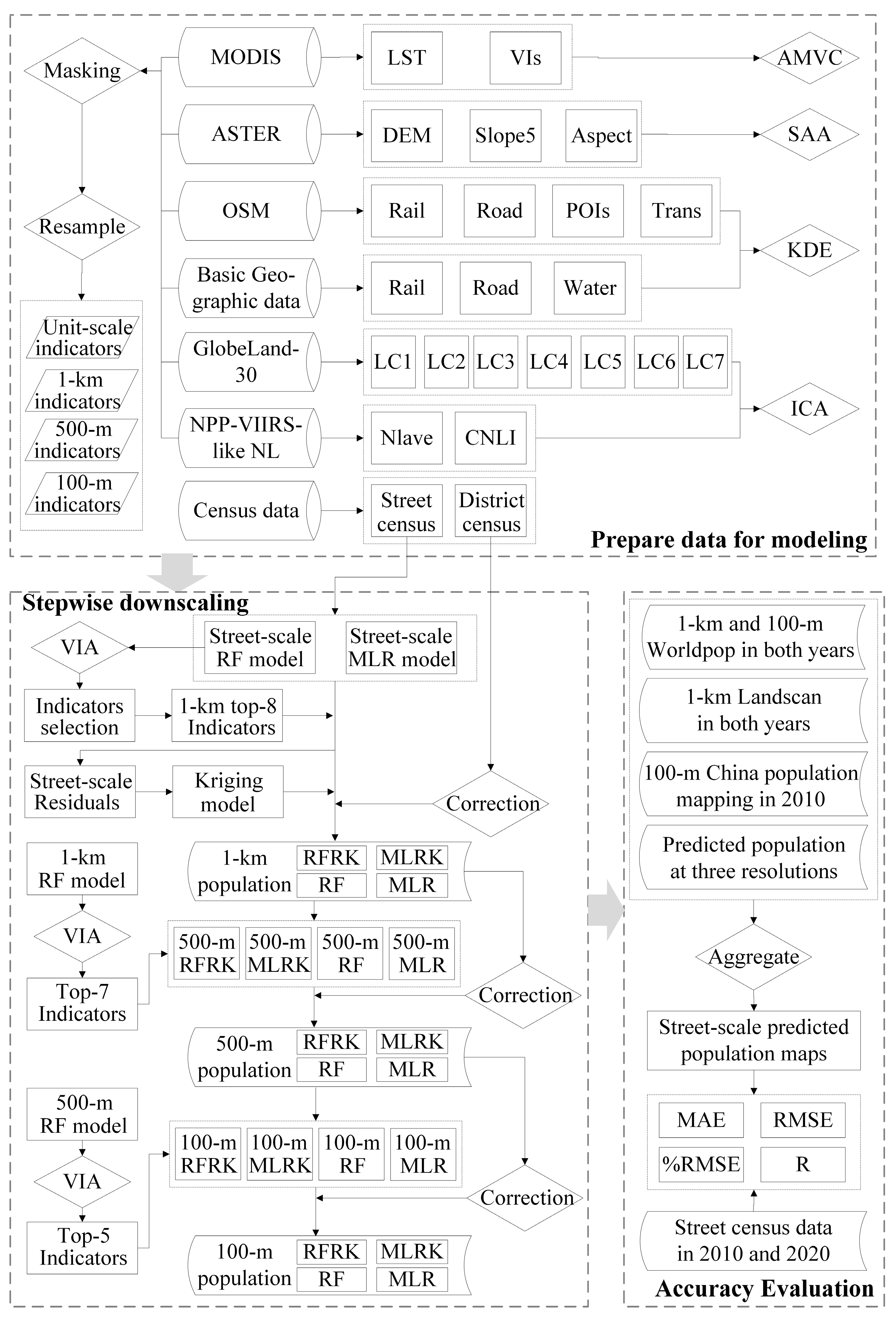
In this experiment, 23 variables derived from six products were employed as the ancillary variables, including DEM, Aspect1, Aspect2, Aspect3, Aspect4, Slope5, LST, NDVI, EVI, NIRv, LC1, LC2, LC3, LC4, LC5, LC6, LC7, NLave, CNLI, POIs, Trans, Rail, and Road. All indicators were preprocessed as described in the data description. In the experiments, considering that there was no population in the water area, population values for water bodies were not included. By repeating the regression and interpolation model, maps of population distribution predicted by multiple linear regression (MLR), random forest regression (RF), multiple linear regression kriging (MLRK) and random forest regression kriging (RFRK) were produced. Random forest regression was also used to sort the predictor variables by their relative importance, and then the top-ranking indicators were selected for the regression model. The library packages “randomForest” and “gstat” were used to implement the RF and kriging methods [51,52]. In the RF model, mtry and ntree were the two crucial parameters which should be optimized [53]. In this study, the value of mtry was set from 1 to 23, and ntree was set as 5, 20, 50, 100, 200, 300, 500, and 1000. Finally, mtry was taken as 4 or 2, whereas the ntree was taken as 500. Given the small amount of street-level census data collected for 2020, two years of data were combined together for regression modeling in the first step of stepwise downscaling. In all regression modeling, 75% and 25% of samples were assigned as the training set and testing set. The R-squared for the two regression models (i.e., RF and MLR) was greater than 0.7 for both the training and testing datasets, with p-values less than 0.01, indicating that the modeling was valid. The multi-resolution population mapping procedure is shown in Figure 3, including the brief data processing, stepwise downscaling, and validation processes. The research mainly comprises the following steps.
(Step 1): Geospatial data (i.e., census data, basic geographic data, and OSM data) and remote sensing data (i.e., MODIS, ASTER, GlobeLand30, NPP-VIIRS-like NL, and WorldPop) were integrated to construct indicators by using kernel density estimation (KDE), slope and aspect analyses (SAA), annual maximum value composite (AMVC), index calculation (ICA), and masking, resampling.
(Step 2): The variable importance analysis (VIA) was realized by random forest at administrative street units. Based on the census data at administrative street units and the top-8 effective indicators (shown in Figure 3), MLR, RF, MLRK, and RFRK (Equation (3)) were developed to estimate the 1 km population distribution, which was corrected by administrative district census data.
(Step 3): The predictor variable’s relative importance was calculated by random forest at 1 km resolution to select effective indicators, including top-7 indicators. Based on the relationship between effective indicators and 1 km population, MLR, RF, MLRK, and RFRK (Equation (4)) were developed to estimate the 500 m population distribution, which was corrected by 1 km corrected population.
(Step 4): The predictor variable’s relative importance was calculated by random forest at 500 m resolution to select effective indicators for two downscaling models, including top-5 indicators. MLR, RF, MLRK, and RFRK (Equation (5)) were developed to estimate the 100 m population distribution, which was corrected by a 500 m corrected population.
(Step 5): To verify the accuracy of the results, the predicted population maps at grid scales (i.e., 1 km, 500 m, and 100 m) in 2010 and 2020 were counted to the street scale for comparison with the actual statistical community population and compared with two WorldPop global population data sets at 1 km and 100 m resolutions, two 1 km LandScan global population database and 100 m China population mapping. Four classical statistical metrics were calculated for each gridded population map, including mean absolute error (MAE) (ten thousand people), root mean square error (RMSE) (ten thousand people), the RMSE divided by the mean census unit count (%RMSE) [34], and correlation coefficient (R).

3. Results

3.1. The Results of Indicators Selections

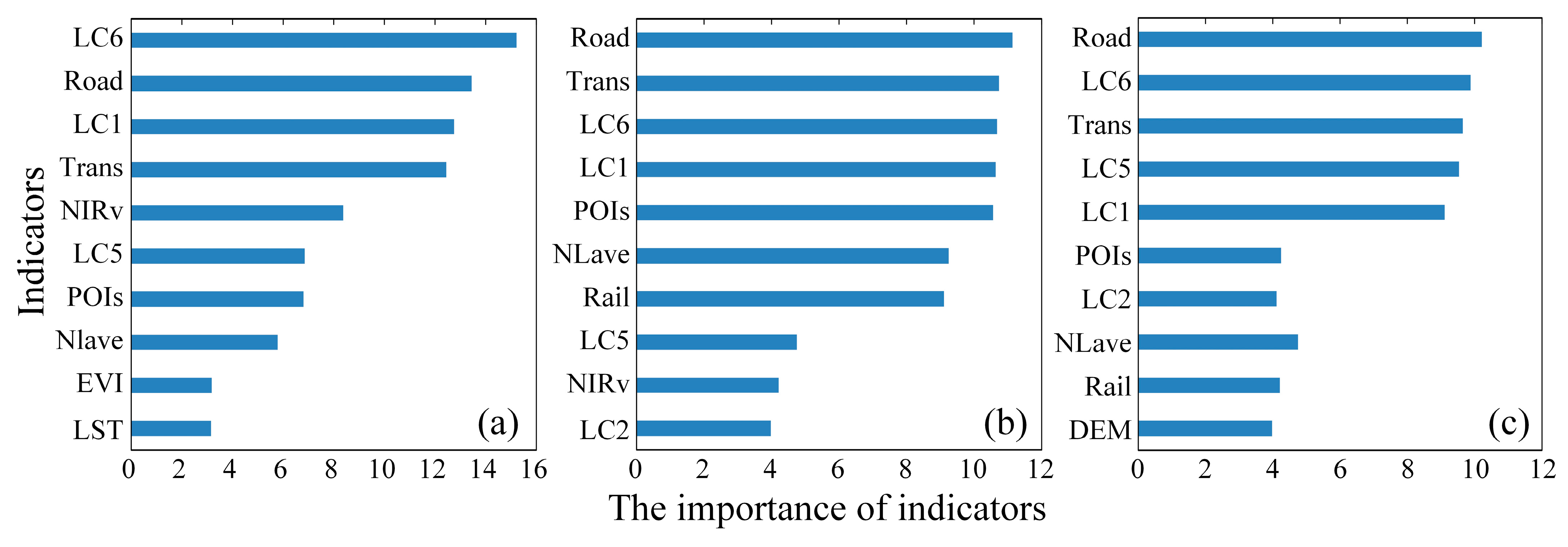
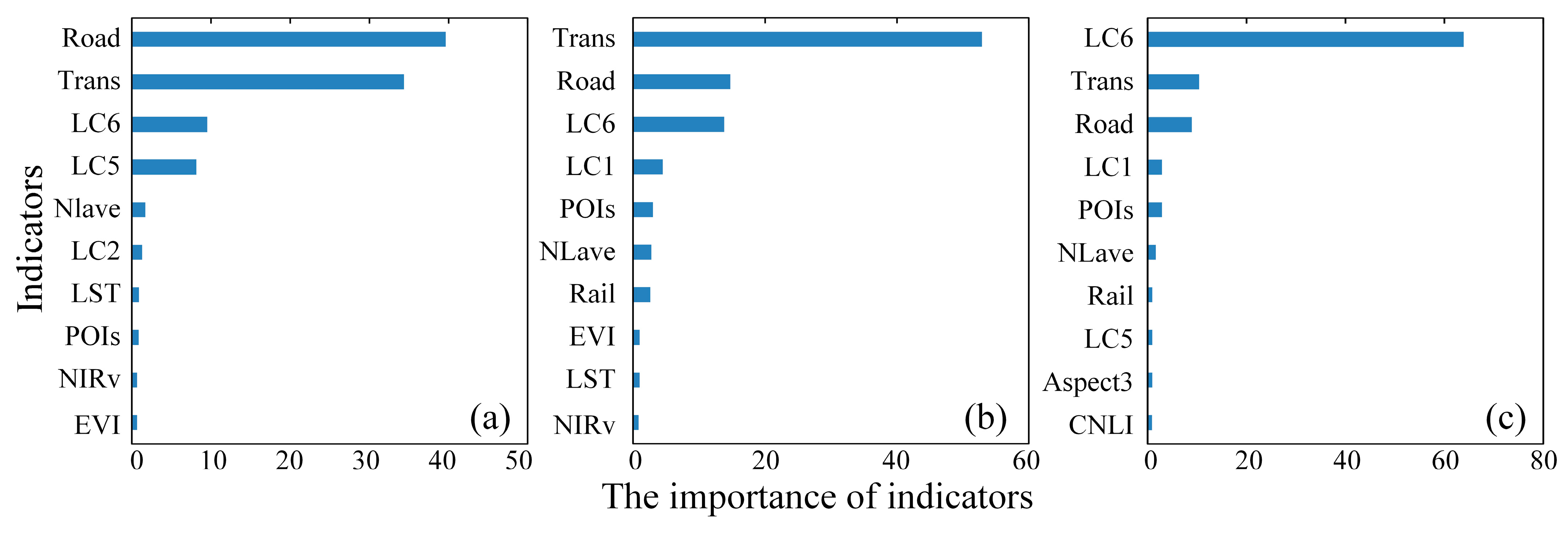
In the experiment, the indicator importance of the independent variables was analyzed in each step of the stepwise strategy by random forest regression method to select the optimal variables for subsequent regression models. The feature importance of the selected independent variables for three steps were displayed in Figure 4.
All of the 23 variables for the 157 administrative street zones were used for fitting and validating the RF model at the street scale. The feature importance of the top-10 variables in three steps is shown in Figure 4. The indicators with an importance greater than five were selected as independent variables. In the first step, there are eight indicators with an importance greater than 5. The variance explained in establishing the model for population prediction of top-8 indicators at the street scale was 85.94%. These top-8 indicators were employed as the ancillary variables to establish the regression models to generate 1 km predictions. LC6, Road, LC1, and transportation (Trans) are the four most important predictors. Among them, the indicator importance of the LC6 is 15.2, and the following variables are Road, LC1 and, Trans with values of 13.4, 12.7, and 12.4. If these top-4 indicators were not involved in the regression model training, the model’s accuracy would drop by more than half. There are seven indicators with importance greater than 5 in Figure 4b; hence, the top-7 indicators were selected at 1 km spatial resolution in the second step, which would be used as the ancillary variables to establish the regression models to generate 500 m predictions. These seven predictors explained 86.12% of the variance of predicted population distribution. At 500 m spatial resolution, the indicator importance of the selected ancillary variables for the third step is displayed in Figure 4c. The top-5 indicators were chosen for establishing the regression models of 100 m resolution, of which the variance explained was 80.57%. LC6 and Road rank in the top three in each step. If both Road and LC6 data did not participate in the model training, the model’s accuracy would decrease by more than 20% in every modeling. Roads serve as a vital means of communication between regions, facilitating the migration of resources, including the population [8]. Artificial land, on the other hand, reflects human activity and is closely linked to population distribution. Therefore, the regression model that combines Road and LC6 data is more effective in estimating population distribution at all three resolutions.

3.2. Gridded Population Mapping

The selected indicators were taken as independent variables to establish the downscaling models in the corresponding step. After the stepwise downscaling with three steps, the gridded multi-resolution population maps were generated using different models at 1 km, 500 m, and 100 m spatial resolutions for the years 2010 and 2020.
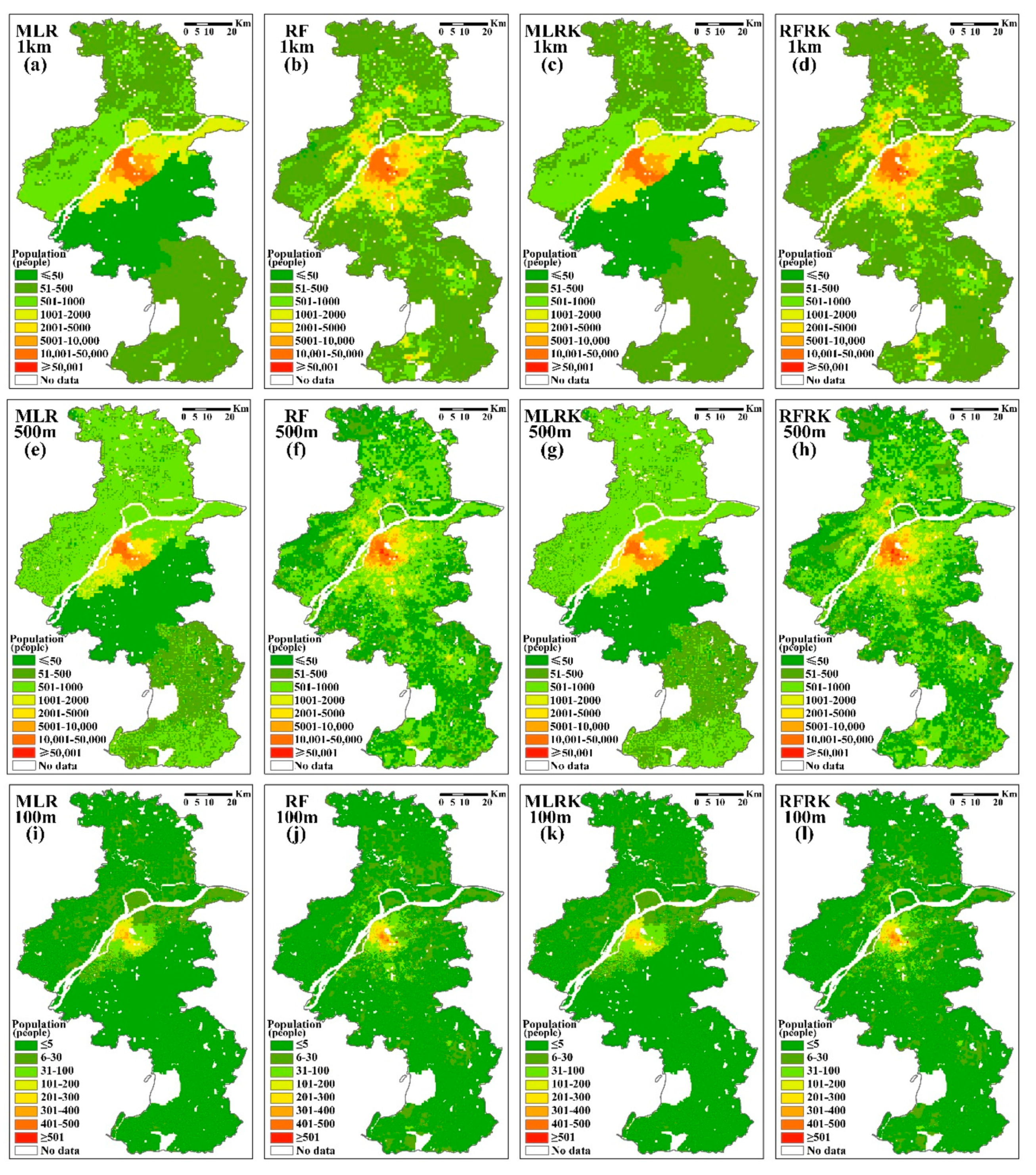
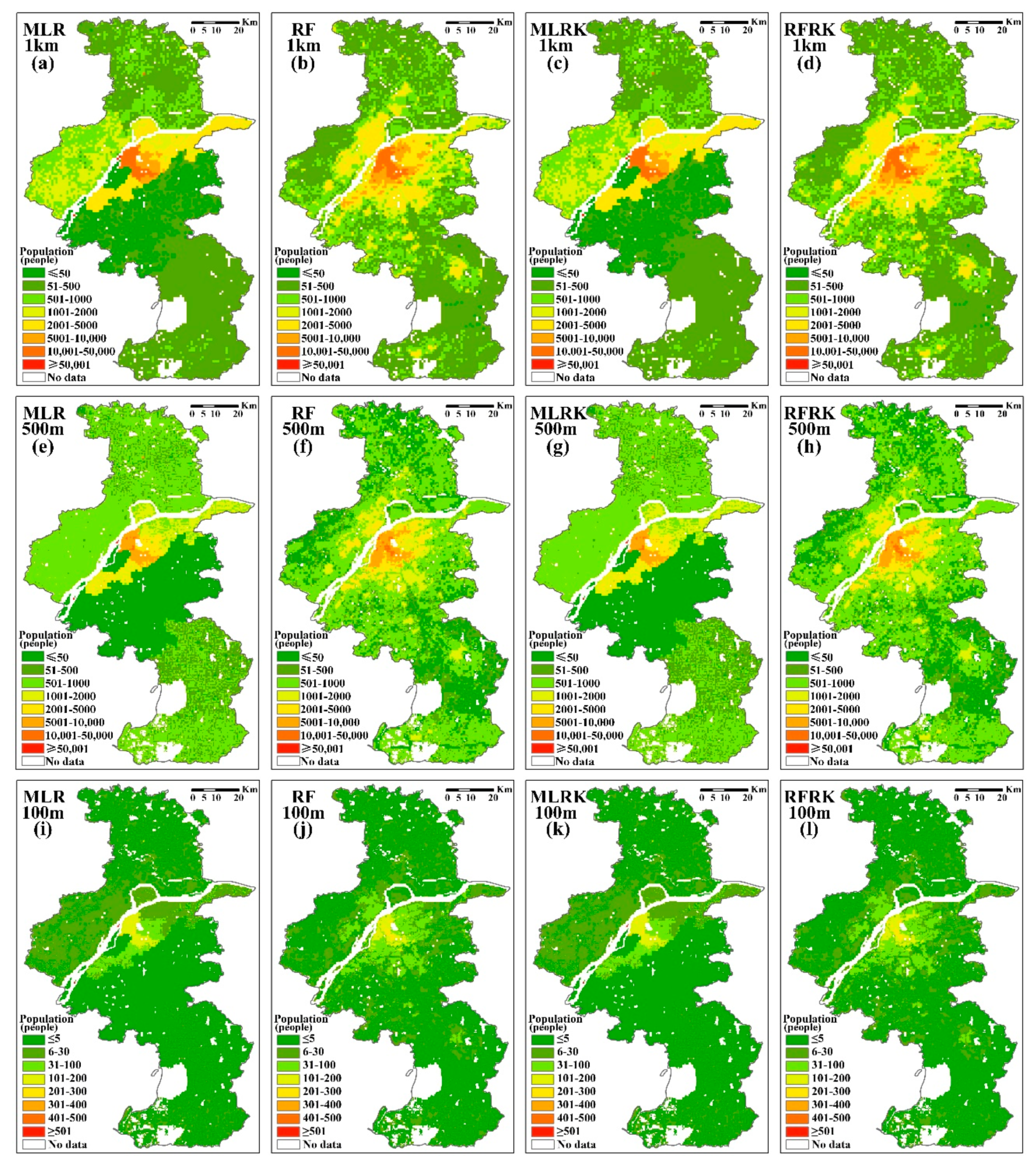
The spatial distribution of the population for the three spatial resolutions in both years is shown in Figure 5 and Figure 6. For all downscaled maps, there is a clear concentration of population, mainly in the central part of the city, with a trend of decreasing from the central city to the surrounding area, which is consistent with the distribution of census data. In 2010, the population was mainly concentrated in the main urban area consisting of Gulou, Xuanwu, Qinhuai, Baixia, Xiaguan, and Jianye districts. Although the population in 2020 remains concentrated in the current main urban area, there has been a significant decrease in population in the city’s center. Instead, there has been a notable spread of population from the center to the surrounding areas, accompanied by the emergence of sub-centers. These areas with densely distributed populations were geographically and economically well-situated for people to live, engage in economic activities, and carry out other daily tasks.
The values of predictions were classified into nine classes for displaying the spatial distribution of the population; however, the range of values for each downscaled result was different. The ranges of values for the RF-based downscaled results were less than the MLR-based models’ ranges. The latter had larger order of magnitude of the maximum values at three different resolutions with less variation. Compared to the RF-based predicted population maps, the predicted results using MLR and MLRK models show less spatial variation within districts and exhibit more distinct district boundaries in both years (see Figure 5 and Figure 6), which could easily lead to underestimation and overestimation, and fail to identify the urban sub-centers. The results from the RFRK model have the largest spatial difference and also revealed the spatial boundaries and could be able to reflect the population clustering phenomenon outside the main urban area, which is particularly evident at 1 km and 500 m resolutions, such as Moling and Dongshan streets in Jiangning District of 2020. The identification of densely populated and sparsely populated areas appears to be largely the same for two RF-based downscaling models at three spatial resolutions. The spatial distribution of the population in Nanjing predicted in this study is consistent with the results of the previous study [54]. However, the gridded population data based on RFRK have more detailed information due to the combined effect of residual interpolation. The population density map can be widely used in tasks such as demographic migration, decision-making, spatial planning and emergency response in Nanjing. The following validation further demonstrates the improved performance of the RFRK method.

3.3. Accuracy Assessment

The population spatialization results predicted by four downscaling models at 1 km, 500 m, and 100 m resolutions were counted to the administrative street scale. The accuracy of various downscaled results for 2010 and 2020 was verified using the street demographic population, respectively.
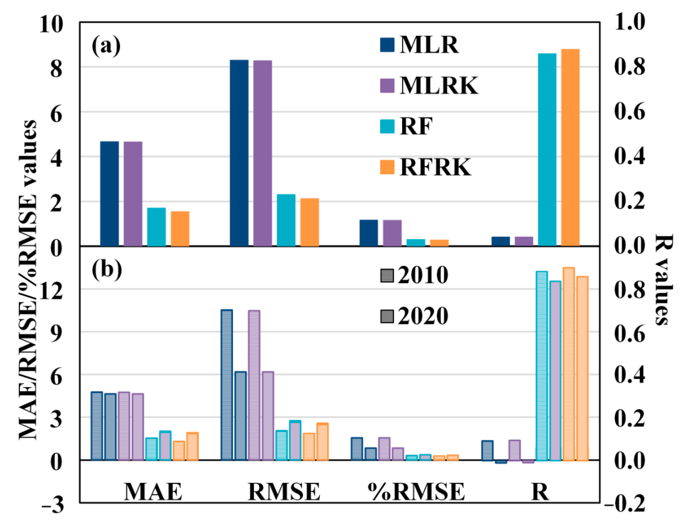
Table 2 shows the calculated four classical statistical metrics for each gridded population map at different spatial resolutions in each year. Overall, the predictions of the population by using the RFRK method had the highest accuracy, followed by the use of RF and MLRK, with the worst accuracy achieved using MLR. At three different spatial resolutions, the 1 km predictions had a higher accuracy than the 500 m and 100 m downscaled results, and the 1 km population distribution map derived from the RFRK model has the highest accuracy in predictions of all cases. Figure 7 displays the average values of four comparison metrics for different downscaling models in different years. The RFRK-based stepwise model produces more accurate predictions than others with an average MAE value of 1.311, an average RMSE value of 1.867, an average %RMSE value of 0.275, and an average R-value of 0.917 in 2010, taking values of 1.869, 2.510, 0.334 and 0.874 in 2020, respectively. For both years, the RFRK approach outperforms the other three downscaling approaches, showing the smallest MAE, RMSE, and %RMSE values of 1.590, 2.189, and 0.304, respectively, and the largest R-value of 0.895 on average. This resulted in a reduction of more than 40% in the first three statistical metrics and an increase of 13% in R.

3.4. Comparison with Population Products

The 1 km and 100 m WorldPop, 1 km LandScan products and 100 m China population mapping were employed to compare with the RFRK-based predicted gridded population of the corresponding resolutions. Table 3 presents the statistical metrics used for comparing the aggregated gridded population with census data, as well as the improvements achieved by RFRK-based predictions in comparison to other data.
As shown in Table 3, it is evident that both WorldPop products and China population mapping outperform the LandScan database. Specifically, China population mapping exhibits the highest accuracy at 100 m resolution, while WorldPop yields the highest accuracy at 1 km resolution. The accuracy of 1 km WorldPop products is better than that of 100 m in both years. At the two spatial resolutions, the average RMSE values of the WorldPop products are 3.262, and 4.747 in 2010 and 2020, respectively, and the MAE values are 2.235 and 3.439, respectively. To analyze the differences between population products and census data, the absolute error between census data and aggregated population predictions of 1 km and 100 m resolutions were calculated at administrative street zones in 2010 and 2020 using WorldPop products as examples, as shown in Figure 8. The RFRK-based population datasets are better than the WorldPop datasets, which appeared to have more overestimations and underestimations. Compared to the three population products, the average MAE values of RFRK-based predictions decreased by 1.259, 2.277 and 1.435, respectively, and average R values increased by 0.206, 0.478 and 0.011, respectively. Each prediction of 1 km and 100 m from the RFRK method has significant improvements with more than a 40% decrease in MAE, RMSE and %RMSE, which means that the designed stepwise RFRK downscaling model has a good predictive ability.

4. Discussion

In order to further discuss the performance of the developed stepwise downscaling method, we analyzed the influences of variables which also made a comparison using the XGBoost method. The errors in stepwise downscaling were discussed which might also be responsible for the differences between methods. Additionally, we explored the potential application of the generated gridded population for monitoring one of the sustainable development goals (SDGs).

4.1. The Influences of Variables

The spatial distribution of the population is influenced by both natural and socioeconomic conditions. In order to explore the feature importance of indicators at three spatial resolutions, XGBoost [55,56] was also employed for the variable importance analysis based on the generated gain scores. The gain scores of indicators for each step were displayed in Figure 9. Comparing the importance of the indicators between the random forest and XGBoost methods, the relative rankings of forest (i.e., LC2) and NIRv are significantly different. The forest is more important in Figure 9a and NIRv is more important in Figure 4a, but both forest and NIRv characterize the vegetation condition. Although the ranking of the importance of the indicators changes, the indicators at the top of the ranking remain largely consistent in the two results from the random forest and XGBoost. In both analyses of the importance of indicators, the variables related to DEM, slope, and aspect were of low importance, which would illustrate that the influence of topographic factors was not significant in Nanjing. This is probably because Nanjing is a hilly area dominated by low hills and gentle hills; its topography is relatively flat, and the population distribution is not obviously clustered in the low-lying areas of the plain. As shown in Figure 4 and Figure 9, the feature importance of NL data is not as high as expected, especially in predicting the population distribution of 100 m resolution. On the one hand, the late overpass time of NPP/VIIRS results in the phenomenon of light loss [57]. Areas without light will also have a population distribution. On the other hand, the original NL data of 500 m were resampled directly into 100 m, and the resampled 100 m NL data might have a large error which would not reflect the population distribution effectively. The artificial land (i.e., LC6) and the road appear to have highly important in all three scales, which are related to their close association with human activity. The overall importance of social factors is higher than natural factors in modeling, indicating a stronger correlation between social factors and the spatial distribution of the population in Nanjing. This may be attributed to the fact that Nanjing is the capital city of the province, and its economic and transport factors exert a more significant influence on the distribution of the population.

4.2. Errors in Stepwise Downscaling

The accuracy of downscaled predictions can be impacted by errors in input data and models used, as noted in previous studies [40]. When comparing different methods, it was observed that the MLR-based approaches had poor accuracy, especially with very low R values. This could be due to the presence of large model errors. In the process of downscaling, the regression relationship established at a coarse spatial resolution will be applied directly to a finer resolution, under the assumption of scale invariance. However, if the regression relationship at finer resolutions changes, the original regression model might have difficulty in accurately characterizing the relationship between the variables, i.e., there may be large model errors, which would lead to a reduction in prediction accuracy at high resolution. The gridded population data based on RF and RFRK outperformed the WorldPop products which also used random forest, probably due to their uses of stepwise modeling and higher-quality indicators. The stepwise modeling allows for the use of different ancillary variables in each regression model, narrowing the range of scales for the scale invariance of the model. The OSM data and night lighting data were applied in both WorldPop and RF-based products; however, the latter integrated the basic geospatial data (such as road and rail) with OSM and replaced the 1 km DMSP/OLS data with the NPP-VIIRS-like NL product at a higher resolution of 500 m. The updated data sources would better reflect the spatial heterogeneity of the population and improve the accuracy of the downscaling model. In China population mapping, which is more accurate than 100 m WorldPop, POIs data were obtained from Baidu Map, China’s largest mobile mapping service provider, which typically provides more accurate data than OSM data for mainland China. The poor performance of LandScan might be due to the fact that the modeling data in China is from the provincial census [8]. Of all the gridded population data, the RFRK-based population predictions are more accurate than all the others. The residual prediction takes into account the spatial distribution characteristics of the variables after the regression analysis, and stepwise modeling allows for the use of different ancillary variables in each regression model, both of which might improve the accuracy of downscaling.
Moreover, in the stepwise downscaling process, the errors can propagate from the previous step to the following steps and can influence the accuracy of the predictions for the next steps. Reducing the errors in the input data of downscaling model is an effective way to restrain error accumulation and thus improve the accuracy of the downscaled results. In this study, on the one hand, the simulation results are corrected to reduce the input errors in the next step of the downscaling process by improving the accuracy of the population prediction in the previous step; on the other hand, the optimal auxiliary variables are selected to reduce the error by controlling the number of input variables. However, there are still some errors based on the downscaled results (as shown in Figure 8). Errors in both the downscaling model and the data used in the model will increase the error in the downscaled predictions. More ways to reduce errors and eliminate error propagation need to be explored in the future.

4.3. Potential Application of Gridded Population

The street-level and district-level census data show general trends in population distribution; however, they could not reflect the population information within administrative units. The gridded population results provide more details of the spatial distribution patterns of the population, such as the identification of the urban sub-centers. Combining the results of the population predictions for both years, it is clear that the population is spreading from the center to the surroundings, which coincides with the facts of Nanjing’s urban expansion in recent years, as well as the built-up area of the city continuously expanding. For example, the growth in the population of Luhe reflects the implementation of Nanjing’s policy of cross-river development and development along the river.
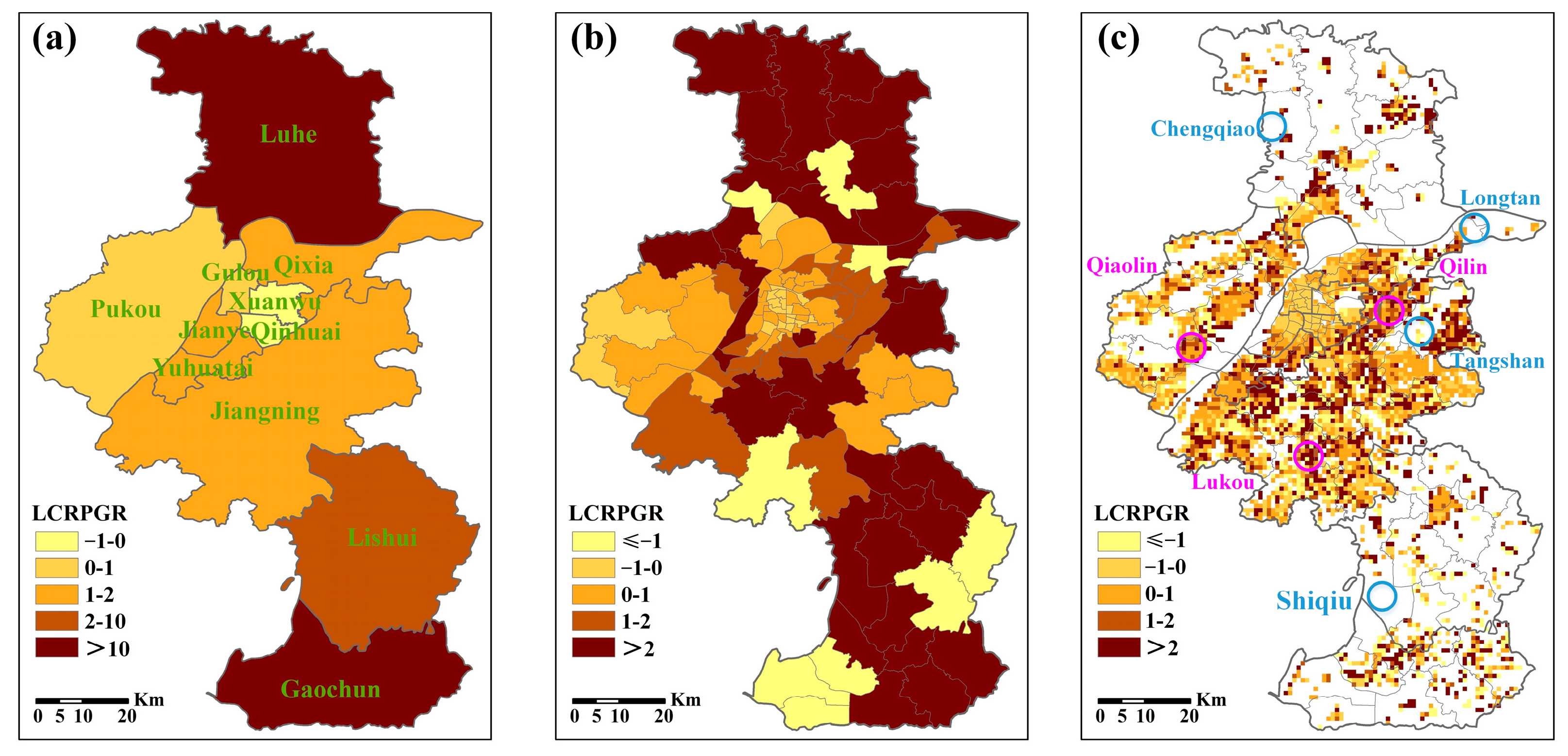
In order to explore the potential applications of gridded population mapping, the downscaled data were used to calculate the SDG 11.3.1 indicator for monitoring the relationship between urban expansion and demographic change from 2010 to 2020. SDG 11.3.1, namely land use efficiency indicator, is the ratio of the land consumption rate (LCR) to the population growth rate (PGR), denoted as LCRPGR, which has been widely used in sustainability analysis of many regions [58,59]. As an initial exploration for future research, the LCR calculation was simplified by replacing the urban built-up area with artificial land information from the GlobeLand30 product. The LCR values at different resolutions were obtained based on the changes in the artificial land in the two years. The district-level PGR was calculated from the district census data, while the street-level PGR was calculated using the 100 m downscaled population due to the absence of a street census. The LCRPGR was figured out by combining the corresponding LCR and PGR at different resolutions, which was divided into five classes, as shown in Figure 10.
The closer the LCRPGR value is to 1, the more coordinated the relationship between land expansion and population growth, indicating a more sustainable development. For three resolutions, more than half of the zones or grids have LCRPGR values between 0 and 2, i.e., 0 < LCRPGR ≤ 1 or 1 < LCRPGR ≤ 2, indicating that the PGR is greater than the LCR and that the LCR is between one and two times the PGR. In Figure 10a, LCRPGR values greater than 2 occur in Luhe, Lishui and Gaochun districts, revealing that land consumption in these regions has increased dramatically and the LCR is much faster than the PGR. LCRPGR greater than 2 at street zones is concentrated in four administrative districts in Figure 10b, with the addition of Jiangning district compared to the district situation. The coordination between the LCR and PGR at the street level is better in Jiangning than in the other three administrative districts. This demonstrates the policy of building development zones in Jiangning of Nanjing, which has gradually become an essential part of Nanjing’s urban area. In Figure 10c, many grids with invalid values appear at 1 km spatial resolution. This is because the artificial land, population and corresponding ratios might appear close to zero at these grids, which would lead to invalid natural logarithm and division calculations in LCR and PGR. For example, in the farmland areas of Chengqiao, Longtan, Tangshan and Shiqiu, where the area of artificial land is zero in 2010 or 2020, the LCRPGR values cannot be obtained in the corresponding regions (as shown in the blue circles in Figure 10c). The 1 km LCRPGR shows that many grids have high values of LCR or PGR, such as the purple circles in Figure 10c, including Qiaolin, Qilin and Lukou, which are vigorously developed areas in Pukou, Jiangning and Lishui districts, respectively. For regions with particularly high LCRPGR values, the sustainability of regional development could be increased by accelerating population clustering through the proper incentives and effectively controlling the intensity of urban expansion [60]. The results of the land use efficiency analyses based on the gridded data all demonstrate the potential for the application of the generated multi-resolution population mapping. Several improved SDG 11.3.1 indicators could be considered in the future to better reflect the land use efficiency.

5. Conclusions

This paper proposes a stepwise downscaling method based on random forest regression kriging, which takes into account the different relationships among variables and varied degrees of indicators’ importance at different scales. At each step of the downscaling process, a random forest model is re-established and optimal indicators are selected through variable importance analysis. The impact of uncertainties in input variables is reduced by choosing and decreasing the number of explanatory variables involved in the regression model. The commonly used random forest algorithm is combined with residual interpolation prediction based on ordinary kriging to improve the accuracy of downscaling results. To demonstrate the effectiveness of this method, a three-stepwise RFRK model was applied to downscale the street-level census data of 2010 and 2020 in Nanjing, China, using 23 indicators from six products as independent variables. The results of variable importance analysis show that artificial land and road data are the two most crucial indicators at three resolutions, due to their close relationship to human activity. The downscaling model combined with Road and LC6 data is more conducive to the predictions of population distribution. Comparison experiments with three other baseline methods (MLR, RF, MLRK) and products (WorldPop, LandScan, and China population mapping) show that the proposed stepwise RFRK method achieves better prediction accuracy than the other baseline methods, with a reduction of more than 40% in MAE, RMSE, and %RMSE, a 21% increase in R, and significant improvement in accuracy compared to WorldPop products. This study demonstrates that the proposed method of fused multisource data can effectively improve the accuracy of population mapping at high spatial resolution. In future work, more socioeconomic data, such as building (e.g., average building height), urban functional areas (such as residential, industrial, and commercial zones), and Tencent location data, will be encouraged in downscaling modeling to enhance the accuracy of population predictions. Additionally, the stepwise method can be extended to downscale census data to fine-resolution populations, such as 10 m and 30 m, by combining it with finer-resolution auxiliary variables.

Author Contributions

Conceptualization, Y.J. (Yan Jin) and Y.J. (Yan Jia); Formal analysis, R.L.; Funding acquisition, Y.J. (Yan Jia); Investigation, R.L. and P.L.; Methodology, Y.J. (Yan Jin); Software, H.F. and Y.L.; Validation, P.L.; Visualization, Y.L.; Writing—original draft, Y.J. (Yan Jin) and R.L.; Writing—review and editing, H.F. and Y.J. (Yan Jia). All authors have read and agreed to the published version of the manuscript.

Funding

This work was supported in part by the National Natural Science Foundation of China under Grants 42001332 and 42201398, the Strategic Priority Research Program of Chinese Academy of Sciences under Grant XDA 20030302, the Natural Science Research of Jiangsu Higher Education Institutions of China under Grant 20KJB170012, and the National Natural Science Foundation of China under Grant 42001375.

Acknowledgments

The authors would like to thank all data producers.

Conflicts of Interest

The authors declare no conflict of interest.

References

  1. Vörösmarty, C.J.; Green, P.; Salisbury, J.; Lammers, R.B. Global Water Resources: Vulnerability from Climate Change and Population Growth. Science 2000, 289, 284–288. [Google Scholar] [CrossRef] [PubMed] [Green Version]
  2. Smith, A.; Bates, P.D.; Wing, O.; Sampson, C.; Quinn, N.; Neal, J. New Estimates of Flood Exposure in Developing Countries Using High-Resolution Population Data. Nat. Commun. 2019, 10, 1814. [Google Scholar] [CrossRef] [PubMed] [Green Version]
  3. Palacios-Lopez, D.; Bachofer, F.; Esch, T.; Marconcini, M.; MacManus, K.; Sorichetta, A.; Zeidler, J.; Dech, S.; Tatem, A.J.; Reinartz, P. High-Resolution Gridded Population Datasets: Exploring the Capabilities of the World Settlement Footprint 2019 Imperviousness Layer for the African Continent. Remote Sens. 2021, 13, 1142. [Google Scholar] [CrossRef]
  4. Xu, Y.; Song, Y.; Cai, J.; Zhu, H. Population mapping in China with Tencent social user and remote sensing data. Appl. Geogr. 2021, 130, 102450. [Google Scholar] [CrossRef]
  5. Sorichetta, A.; Hornby, G.M.; Stevens, F.R.; Gaughan, A.E.; Linard, C.; Tatem, A.J. High-Resolution Gridded Population Datasets for Latin America and the Caribbean in 2010, 2015, and 2020. Sci. Data 2015, 2, 150045. [Google Scholar] [CrossRef] [Green Version]
  6. Leyk, S.; Gaughan, A.E.; Adamo, S.B.; de Sherbinin, A.; Balk, D.; Freire, S.; Rose, A.; Stevens, F.R.; Blankespoor, B.; Frye, C.; et al. The Spatial Allocation of Population: A Review of Large-Scale Gridded Population Data Products and Their Fitness for Use. Earth Syst. Sci. Data 2019, 11, 1385–1409. [Google Scholar] [CrossRef] [Green Version]
  7. Li, K.; Chen, Y.; Li, Y. The Random Forest-Based Method of Fine-Resolution Population Spatialization by Using the International Space Station Nighttime Photography and Social Sensing Data. Remote Sens. 2018, 10, 1650. [Google Scholar] [CrossRef] [Green Version]
  8. Wang, Y.; Huang, C.; Zhao, M.; Hou, J.; Zhang, Y.; Gu, J. Mapping the Population Density in Mainland China Using NPP/VIIRS and Points-Of-Interest Data Based on a Random Forests Model. Remote Sens. 2020, 12, 3645. [Google Scholar] [CrossRef]
  9. Stokes, E.; Seto, K. Characterizing urban infrastructural transitions for the Sustainable Development Goals using multi-temporal land, population, and nighttime light data. Remote Sens. Environ. 2019, 234, 111430. [Google Scholar] [CrossRef]
  10. Tuholske, C.; Gaughan, A.E.; Sorichetta, A.; de Sherbinin, A.; Bucherie, A.; Hultquist, C.; Stevens, F.; Kruczkiewicz, A.; Huyck, C.; Yetman, G. Implications for Tracking SDG Indicator Metrics with Gridded Population Data. Sustainability 2021, 13, 7329. [Google Scholar] [CrossRef]
  11. Wu, S.; Qiu, X.; Wang, L. Population Estimation Methods in GIS and Remote Sensing: A Review. GIScience Remote Sens. 2005, 42, 80–96. [Google Scholar] [CrossRef]
  12. Bo, Z.Q.; Wang, J.L.; Yang, F. Research progress in spatialization of population data. Prog. Geogr. 2013, 32, 1692–1702. [Google Scholar] [CrossRef]
  13. Bhaduri, B.; Bright, E.; Coleman, P.; Urban, M.L. LandScan USA: A High-Resolution Geospatial and Temporal Modeling Approach for Population Distribution and Dynamics. GeoJournal 2007, 69, 103–117. [Google Scholar] [CrossRef]
  14. Murakami, D.; Yamagata, Y. Estimation of Gridded Population and GDP Scenarios with Spatially Explicit Statistical Downscaling. Sustainability 2019, 11, 2106. [Google Scholar] [CrossRef] [Green Version]
  15. Dobson, J.E.; Bright, E.A.; Coleman, P.R.; Durfee, R.C.; Worley, B.A. LandScan: A Global Population Database for Estimating Populations at Risk. Photogramm. Eng. Remote Sens. 2000, 66, 849–857. [Google Scholar]
  16. Zhao, X.; Xia, N.; Xu, Y.; Huang, X.; Li, M. Mapping Population Distribution Based on XGBoost Using Multisource Data. IEEE J. Sel. Top. Appl. Earth Obs. Remote Sens. 2021, 14, 11567–11580. [Google Scholar] [CrossRef]
  17. Yin, C.; Shi, Y.; Wang, H.; Wu, J. Disaggregation of an Urban Population with M_IDW Interpolation and Building Information. J. Urban Plan. Dev. 2015, 141, 04014012. [Google Scholar] [CrossRef]
  18. Goodchild, M.F.; Anselin, L.; Deichmann, U. A Framework for the Areal Interpolation of Socioeconomic Data. Environ. Plan. Econ. Space 1993, 25, 383–397. [Google Scholar] [CrossRef]
  19. Cai, Q.; Rushton, G.; Bhaduri, B.; Bright, E.; Coleman, P. Estimating Small-area Populations By Age and Sex Using Spatial Interpolation and Statistical Inference Methods. Trans. GIS 2006, 10, 577–598. [Google Scholar] [CrossRef]
  20. Zandbergen, P.A.; Ignizio, D.A. Comparison Of Dasymetric Mapping Techniques For Small-Area Population Estimates. Cartogr. Geogr. Inf. Sci. 2010, 37, 199–214. [Google Scholar] [CrossRef]
  21. Doxsey-Whitfield, E.; MacManus, K.; Adamo, S.B.; Pistolesi, L.; Squires, J.; Borkovska, O.; Baptista, S.R. Taking Advantage of the Improved Availability of Census Data: A First Look at the Gridded Population of the World, Version 4. Pap. Appl. Geogr. 2015, 1, 226–234. [Google Scholar] [CrossRef]
  22. Zhang, C.; Qiu, F. A Point-Based Intelligent Approach to Areal Interpolation. Prof. Geogr. 2011, 63, 262–276. [Google Scholar] [CrossRef]
  23. Su, M.-D.; Lin, M.-C.; Hsieh, H.-I.; Tsai, B.-W.; Lin, C.-H. Multi-Layer Multi-Class Dasymetric Mapping to Estimate Population Distribution. Sci. Total Environ. 2010, 408, 4807–4816. [Google Scholar] [CrossRef] [PubMed]
  24. Bao, W.; Gong, A.; Zhao, Y.; Chen, S.; Ba, W.; He, Y. High-Precision Population Spatialization in Metropolises Based on Ensemble Learning: A Case Study of Beijing, China. Remote Sens. 2022, 14, 3654. [Google Scholar] [CrossRef]
  25. Ma, T.; Zhou, C.; Pei, T.; Haynie, S.; Fan, J. Quantitative estimation of urbanization dynamics using time series of DMSP/OLS nighttime light data: A comparative case study from China’s cities. Remote Sens. Environ. 2012, 124, 99–107. [Google Scholar] [CrossRef]
  26. Zeng, C.; Zhou, Y.; Wang, S.; Yan, F.; Zhao, Q. Population spatialization in China based on night-time imagery and land use data. Int. J. Remote Sens. 2011, 32, 9599–9620. [Google Scholar] [CrossRef]
  27. Tu, W.; Liu, Z.; Du, Y.; Yi, J.; Liang, F.; Wang, N.; Qian, J.; Huang, S.; Wang, H. An Ensemble Method to Generate High-Resolution Gridded Population Data for China from Digital Footprint and Ancillary Geospatial Data. Int. J. Appl. Earth Obs. Geoinf. 2022, 107, 102709. [Google Scholar] [CrossRef]
  28. Cheng, L.; Wang, L.; Feng, R.; Yan, J. Remote Sensing and Social Sensing Data Fusion for Fine-Resolution Population Mapping With a Multimodel Neural Network. IEEE J. Sel. Top. Appl. Earth Obs. Remote Sens. 2021, 14, 5973–5987. [Google Scholar] [CrossRef]
  29. Wang, L.; Fan, H.; Wang, Y. Fine-Resolution Population Mapping from International Space Station Nighttime Photography and Multisource Social Sensing Data Based on Similarity Matching. Remote Sens. 2019, 11, 1900. [Google Scholar] [CrossRef] [Green Version]
  30. Chu, H.-J.; Yang, C.-H.; Chou, C.C. Adaptive Non-Negative Geographically Weighted Regression for Population Density Estimation Based on Nighttime Light. ISPRS Int. J. Geo-Inf. 2019, 8, 26. [Google Scholar] [CrossRef] [Green Version]
  31. He, M.; Xu, Y.; Li, N. Population Spatialization in Beijing City Based on Machine Learning and Multisource Remote Sensing Data. Remote Sens. 2020, 12, 1910. [Google Scholar] [CrossRef]
  32. Zhao, S.; Liu, Y.; Zhang, R.; Fu, B. China’s Population Spatialization Based on Three Machine Learning Models. J. Clean. Prod. 2020, 256, 120644. [Google Scholar] [CrossRef]
  33. Zhou, Y.; Ma, M.; Shi, K.; Peng, Z. Estimating and Interpreting Fine-Scale Gridded Population Using Random Forest Regression and Multisource Data. ISPRS Int. J. Geo-Inf. 2020, 9, 369. [Google Scholar] [CrossRef]
  34. Stevens, F.R.; Gaughan, A.E.; Linard, C.; Tatem, A.J. Disaggregating Census Data for Population Mapping Using Random Forests with Remotely-Sensed and Ancillary Data. PLoS ONE 2015, 10, e0107042. [Google Scholar] [CrossRef] [PubMed] [Green Version]
  35. Kim, H.; Yao, X. Pycnophylactic interpolation revisited: Integration with the dasymetric-mapping method. Int. J. Remote Sens. 2010, 31, 5657–5671. [Google Scholar] [CrossRef]
  36. Zoraghein, H.; Leyk, S. Enhancing areal interpolation frameworks through dasymetric refinement to create consistent population estimates across censuses. Int. J. GIS 2018, 32, 1948–1976. [Google Scholar] [CrossRef]
  37. Cockx, K.; Canters, F. Incorporating spatial non-stationarity to improve dasymetric mapping of population. Appl. Geogr. 2015, 63, 220–230. [Google Scholar] [CrossRef]
  38. Roni, R.; Jia, P. An Optimal Population Modeling Approach Using Geographically Weighted Regression Based on High-Resolution Remote Sensing Data: A Case Study in Dhaka City, Bangladesh. Remote Sens. 2020, 12, 1184. [Google Scholar] [CrossRef] [Green Version]
  39. Wang, M.; Wang, Y.; Li, B.; Cai, Z.; Kang, M. A Population Spatialization Model at the Building Scale Using Random Forest. Remote Sens. 2022, 14, 1811. [Google Scholar] [CrossRef]
  40. Ge, Y.; Jin, Y.; Stein, A.; Chen, Y.; Wang, J.; Wang, J.; Cheng, Q.; Bai, H.; Liu, M.; Atkinson, P.M. Principles and Methods of Scaling Geospatial Earth Science Data. Earth-Sci. Rev. 2019, 197, 102897. [Google Scholar] [CrossRef]
  41. Mei, Y.; Gui, Z.; Wu, J.; Peng, D.; Li, R.; Wu, H.; Wei, Z. Population spatialization with pixel-level attribute grading by considering scale mismatch issue in regression modeling. Geo-Spatial Inf. Sci. 2022, 25, 365–382. [Google Scholar] [CrossRef]
  42. Qiu, G.; Bao, Y.; Yang, X.; Wang, C.; Ye, T.; Stein, A.; Jia, P. Local Population Mapping Using a Random Forest Model Based on Remote and Social Sensing Data: A Case Study in Zhengzhou, China. Remote Sens. 2020, 12, 1618. [Google Scholar] [CrossRef]
  43. Yin, X.; Li, P.; Feng, Z.; Yang, Y.; You, Z.; Xiao, C. Which Gridded Population Data Product Is Better? Evidences from Mainland Southeast Asia (MSEA). ISPRS Int. J. Geo-Inf. 2021, 10, 681. [Google Scholar] [CrossRef]
  44. Jin, Y.; Hao, Z.; Chen, J.; He, D.; Tian, Q.; Mao, Z.; Pan, D. Retrieval of Urban Aerosol Optical Depth from Landsat 8 OLI in Nanjing, China. Remote Sens. 2021, 13, 415. [Google Scholar] [CrossRef]
  45. Xiang, Y.; Tang, Y.; Wang, Z.; Peng, C.; Huang, C.; Dian, Y.; Teng, M.; Zhou, Z. Seasonal Variations of the Relationship between Spectral Indexes and Land Surface Temperature Based on Local Climate Zones: A Study in Three Yangtze River Megacities. Remote Sens. 2023, 15, 870. [Google Scholar] [CrossRef]
  46. Chen, Z.; Yu, B.; Yang, C.; Zhou, Y.; Yao, S.; Qian, X.; Wang, C.; Wu, B.; Wu, J. An Extended Time Series (2000–2018) of Global NPP-VIIRS-like Nighttime Light Data from a Cross-Sensor Calibration. Earth Syst. Sci. Data 2021, 13, 889–906. [Google Scholar] [CrossRef]
  47. Gao, B.; Huang, Q.; He, C.; Ma, Q. Dynamics of Urbanization Levels in China from 1992 to 2012: Perspective from DMSP/OLS Nighttime Light Data. Remote Sens. 2015, 7, 1721–1735. [Google Scholar] [CrossRef] [Green Version]
  48. Ye, T.; Zhao, N.; Yang, X.; Ouyang, Z.; Liu, X.; Chen, Q.; Hu, K.; Yue, W.; Qi, J.; Li, Z.; et al. Improved population mapping for China using remotely sensed and points-of-interest data within a random forests model. Sci. Total Environ. 2019, 658, 936–946. [Google Scholar] [CrossRef]
  49. Belgiu, M.; Drăguţ, L. Random Forest in Remote Sensing: A Review of Applications and Future Directions. ISPRS J. Photogramm. Remote Sens. 2016, 114, 24–31. [Google Scholar] [CrossRef]
  50. Pouladi, N.; Møller, A.B.; Tabatabai, S.; Greve, M.H. Mapping Soil Organic Matter Contents at Field Level with Cubist, Random Forest and Kriging. Geoderma 2019, 342, 85–92. [Google Scholar] [CrossRef]
  51. Liaw, A.; Wiener, M. Randomforest: Breiman and Cutler’s Random Forests for Classification and Regression; RpackageVersion 4.7-1.1; 2022. Available online: https://cran.r-project.org/web/packages/randomForest/ (accessed on 7 July 2022).
  52. Pebesma, E.; Graeler, B. Gstat: Spatial and Spatio-Temporal Geostatistical Modelling, Prediction and Simulation; RpackageVersion 2.1-0; 2022. Available online: https://cran.r-project.org/web/packages/gstat/ (accessed on 12 December 2022).
  53. Yang, W.; Wan, X.; Liu, M.; Zheng, D.; Liu, H. A two-level random forest model for predicting the population distributions of urban functional zones: A case study in Changsha, China. Sustain. Cities Soc. 2023, 88, 104297. [Google Scholar] [CrossRef]
  54. Chen, Y.; Zhang, R.; Ge, Y.; Jin, Y.; Xia, Z. Downscaling census data for gridded population mapping with geographically weighted area-to-point regression kriging. IEEE Access 2019, 7, 149132–149141. [Google Scholar] [CrossRef]
  55. Abdullah, A.Y.M.; Masrur, A.; Adnan, M.S.G.; Baky, M.A.A.; Hassan, Q.K.; Dewan, A. Spatio-Temporal Patterns of Land Use/Land Cover Change in the Heterogeneous Coastal Region of Bangladesh between 1990 and 2017. Remote Sens. 2019, 11, 790. [Google Scholar] [CrossRef] [Green Version]
  56. Georganos, S.; Grippa, T.; Vanhuysse, S.; Lennert, M.; Shimoni, M.; Kalogirou, S.; Wolff, E. Less is more: Optimizing classification performance through feature selection in a very-high-resolution remote sensing object-based urban application. Gisci. Remote Sens. 2018, 55, 221–242. [Google Scholar] [CrossRef]
  57. Li, X.; Levin, N.; Xie, J.; Li, D. Monitoring Hourly Night-Time Light by an Unmanned Aerial Vehicle and Its Implications to Satellite Remote Sensing. Remote Sens. Environ. 2020, 247, 111942. [Google Scholar] [CrossRef]
  58. Gao, K.; Yang, X.; Wang, Z.; Zhang, H.; Huang, C.; Zeng, X. Spatial Sustainable Development Assessment Using Fusing Multisource Data from the Perspective of Production-Living-Ecological Space Division: A Case of Greater Bay Area, China. Remote Sens. 2022, 14, 2772. [Google Scholar] [CrossRef]
  59. Calka, B.; Orych, A.; Bielecka, E.; Mozuriunaite, S. The Ratio of the Land Consumption Rate to the Population Growth Rate: A Framework for the Achievement of the Spatiotemporal Pattern in Poland and Lithuania. Remote Sens. 2022, 14, 1074. [Google Scholar] [CrossRef]
  60. Wang, Y.; Huang, C.; Feng, Y.; Zhao, M.; Gu, J. Using Earth Observation for Monitoring SDG 11.3.1-Ratio of Land Consumption Rate to Population Growth Rate in Mainland China. Remote Sens. 2020, 12, 357. [Google Scholar] [CrossRef] [Green Version]
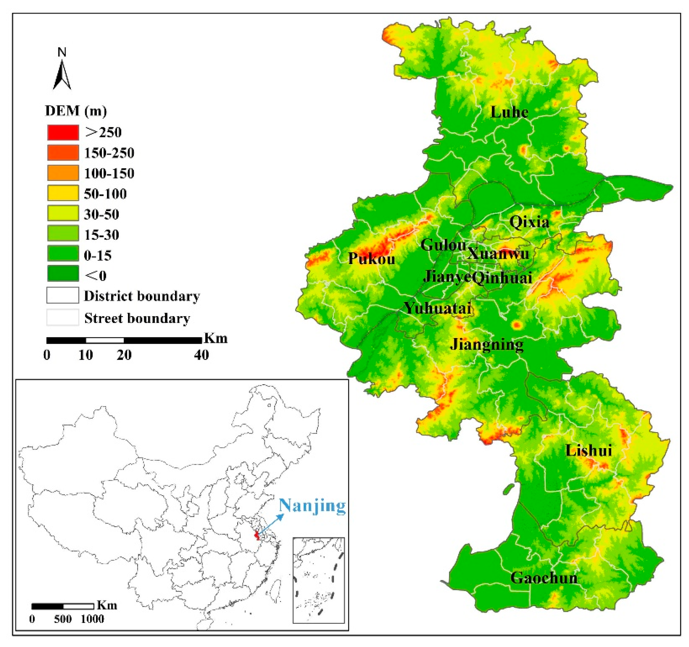
Figure 1. Nanjing Study area.
Remotesensing 15 01947 g001
Figure 2. Census data at administrative street zones of Nanjing in (a) 2010 and (b) 2020. The absent street census in 2020 were supplemented by the corresponding district census, shown in purple to lighter purples.
Remotesensing 15 01947 g002
Figure 3. Flowchart of the multi-resolution population mapping methodology.
Remotesensing 15 01947 g003
Figure 4. The feature importance of the top-10 indicators in three steps: (a) 1 km regression models; (b) 500 m regression models; (c) 100 m regression models.
Remotesensing 15 01947 g004
Figure 5. The spatial distribution of downscaled population in 2010 (ad) at 1 km resolution, (eh) at 500 m resolution, and (il) at 100 m resolution by using MLR, RF, MLRK, and RFRK methods, respectively.
Remotesensing 15 01947 g005
Figure 6. The spatial distribution of downscaled population in 2020 (ad) at 1 km resolution, (eh) at 500 m resolution, and (il) at 100 m resolution by using MLR, RF, MLRK, and RFRK methods, respectively.
Remotesensing 15 01947 g006
Figure 7. Four comparison metrics for different downscaling models in (a) both years and (b) single year. The average values were calculated in both years.
Remotesensing 15 01947 g007
Figure 8. The absolute error at administrative street zones between census data and aggregated population predictions of 1 km and 100 m resolutions in 2010 and 2020: (ad) WorldPop products; (eh) RFRK-based downscaled results. The absent street zones in 2020 were filled with aggregated WorldPop data or aggregated RFRK-based predictions (marked as RFK).
Remotesensing 15 01947 g008
Figure 9. The feature importance of the top-10 indicators in three steps by using XGBoost: (a) 1 km regression models; (b) 500 m regression models; (c) 100 m regression models.
Remotesensing 15 01947 g009
Figure 10. The LCRPGR valued in Nanjing in 2010–2020. The spatial distribution at different resolutions: (a) administrative district zones by using census data; (b) administrative street zones by using 100 m downscaled population based on RFRK; (c) 1 km resolution by using 1 km downscaled population based on RFRK.
Remotesensing 15 01947 g010
Table 2. Four statistical metrics for each gridded population map at different spatial resolutions in 2010 and 2020.
20102020
MAERMSE%RMSERMAERMSE%RMSER
1 kmMLR5.02011.2591.6560.0854.7096.3200.842−0.031
RF1.4852.0080.2950.9031.8842.6130.3480.860
MLRK5.00811.2161.6490.0864.7076.3180.841−0.031
RFRK1.2711.8150.2670.9221.7902.4520.3270.880
500 mMLR4.74810.4411.5350.0954.6966.2070.8270.008
RF1.5482.0820.3060.8952.0032.6880.3580.852
MLRK4.72810.3671.5240.0984.6956.2060.8260.008
RFRK1.3291.9030.2800.9131.8982.5160.3350.873
100 mMLR4.74410.3781.5260.1004.7246.2780.836−0.009
RF1.5532.0760.3050.8962.0322.7500.3660.845
MLRK4.72710.3041.5150.1024.7226.2770.836−0.009
RFRK1.3331.8840.2770.9151.9192.5620.3410.868
Table 3. Four statistical metrics for 1 km and 100 m WorldPop products in Nanjing of 2010, 2020, and both years.
WPop 1 kmWPop 100 mLPopCPopImprovements of RFRK
2010202020102020201020202010WpopLPopCPop
MAE2.2313.7532.2383.1242.9534.6612.768↓ 1.259↓ 2.277↓ 1.435
RMSE3.2315.1793.2924.3144.3216.3193.677↓ 1.826↓ 3.186↓ 1.793
%RMSE0.4750.6900.4840.5750.6350.8410.541↓ 0.253↓ 0.442↓ 0.264
R0.8200.5090.8150.6170.5870.2600.904↑ 0.206↑ 0.478↑ 0.011
Note: WorldPop, LandScan and China population mapping are noted as WPop, LPop and CPop. The arrows ↓ and ↑ denote increase and decrease, respectively.
Disclaimer/Publisher’s Note: The statements, opinions and data contained in all publications are solely those of the individual author(s) and contributor(s) and not of MDPI and/or the editor(s). MDPI and/or the editor(s) disclaim responsibility for any injury to people or property resulting from any ideas, methods, instructions or products referred to in the content.