Potential of Optical Spaceborne Sensors for the Differentiation of Plastics in the Environment

Abstract

Plastics are part of our everyday life, as they are versatile materials and can be produced inexpensively. Approximately 10 Gt of plastics have been produced to date, of which the majority have been accumulated in landfills or have been spread into the terrestrial and aquatic environment in an uncontrolled way. Once in the environment, plastic litter—in its large form or degraded into microplastics—causes several harms to a variety of species. Thus, the detection of plastic waste is a pressing research question in remote sensing. The majority of studies have used Sentinel-2 or WorldView-3 data and empirically explore the usefulness of the given spectral channels for the detection of plastic litter in the environment. On the other hand, laboratory infrared spectroscopy is an established technique for the differentiation of plastic types based on their type-specific absorption bands; the potential of hyperspectral remote sensing for mapping plastics in the environment has not yet been fully explored. In this study, reflectance spectra of the five most commonly used plastic types were used for spectral sensor simulations of ten selected multispectral and hyperspectral sensors. Their signals were classified in order to differentiate between the plastic types as would be measured in nature and to investigate sensor-specific spectral configurations neglecting spatial resolution limitations. Here, we show that most multispectral sensors are not able to differentiate between plastic types, while hyperspectral sensors are. To resolve absorption bands of plastics with multispectral sensors, the number, position, and width of the SWIR channels are decisive for a good classification of plastics. As ASTER and WorldView-3 had/have narrow SWIR channels that match with diagnostic absorption bands of plastics, they yielded outstanding results. Central wavelengths at 1141, 1217, 1697, and 1716 nm, in combination with narrow bandwidths of 10–20 nm, have the highest capability for plastic differentiation.

1. Introduction

Plastics designate a group of (semi-)synthetic polymers and combine excellent material properties. They are used for manifold purposes as they are cheap, durable, water resistant, strong, and light. Their mass production and use began in ~1950 with an annual global production of 2 Mt, which has increased to 381 Mt in 2015 [1]. This has resulted in a cumulative global production of ~10 Gt over the last 70 years. Many plastic types have been synthesized to date but only seven are used regularly and account for 95.1% of total plastic production: high-density polyethylene (PE-HD), low-density polyethylene (PE-LD), polyethylene terephthalate (PET), polypropylene (PP), polyurethane (PU), polystyrene (PS), and polyvinyl chloride (PVC) [1]. Packaging is their main application, accounting for almost 45% of all plastic consumption [1]. This implies that most of the plastics produced are usually only used once [2].

The outstanding material properties become a problem once plastics are released into the environment as litter. As all regularly used plastics are non-biodegradable, their total degradation takes several hundred years [3]. An accumulation of plastic debris at disposal sites or in the environment is therefore inevitable. Approximately 79% of all plastics ever produced have been accumulated at disposal sites or in the environment [1]. Consequently, nearly 8 Gt of plastics can nowadays be expected to be in landfills or the environment, where soils and oceans form a final sink [4]. Many studies highlight the accumulation of plastic debris in the marine and coastal environment, with estimates of 60–80% of the total waste being plastics [5]. For the terrestrial environment, it has been determined that more than 50% of all waste are plastics [6]. Plastic waste occurs globally since it is easily distributed by wind and water [7,8]. The persistence of plastics causes an enduring degradation of larger objects into microplastics and the release of problematic substances for long times, which threatens the environment and its organisms [4,9,10]. Moreover, human health is affected by plastics and their additives, even in the natural environment [11,12]. This emphasizes the need of recovering plastic waste before it enters water bodies or decays on land.

The long-chain polymer structure of plastics, consisting of many repetitions of identical monomers with a limited variety of atoms, forms many absorption bands in their spectral reflectance signatures [13]. These absorption bands are relatively narrow and deep compared to natural materials that have smoother signals, such as vegetation or soils. The characteristic and distinct absorption bands in the infrared spectra of plastics are found for wavelengths greater than ~900 nm, i.e., mainly in the short-wave infrared (SWIR) part of the electromagnetic spectrum. This makes them ideal for spectroscopy, as each plastic type has diagnostic absorption bands at specific wavelengths [14,15,16]. Infrared spectroscopy has been used for many decades, e.g., [17,18,19], while applications are found in waste management and the recycling industry. The findings from laboratory infrared spectroscopy applied to remote sensing could be demonstrated for various hydrocarbons at an early stage [20], and have since been intensively researched. The Hydrocarbon Index is capable of detecting hydrocarbons without differentiation using hyperspectral sensors [21]. Whether the benefits of laboratory spectroscopy for plastic differentiation are applicable for spaceborne sensors has recently been studied, e.g., [22,23,24,25,26,27,28,29,30,31,32,33].

Spaceborne remote sensing has the potential to scan large areas continuously. Its application for plastics is young, yet promising, and has the potential to create a global map of plastic debris in the environment [29]. So far, this has not yet been made, as there are only a few satellites with which plastics can be detected according to recent knowledge. The majority of studies use Sentinel-2 or WorldView-3 data and empirically explore the usefulness of the given spectral channels for the identification and differentiation of plastic litter in the environment, e.g., [27,32]. However, there remains a gap regarding a systematic evaluation of spectral configurations of the most common optical spaceborne sensors for their suitability of differentiating plastic types.

To address this gap, our study examines the capability of former and present optical spaceborne multispectral (Dove/Flock PlanetScope, Landsat 5 TM/7 ETM+, Pléiades-HR 1A/1B HiRI, Sentinel-2 MSI, Terra ASTER, Terra/Aqua MODIS, and WorldView-3 WV110) and hyperspectral sensors (EnMAP HSI, EO-1 Hyperion, and PRISMA HYC) to detect and differentiate plastics in the environment. We used infrared reflectance signals of the most commonly used plastic types to simulate their reflectance signals as would be measured on various surface materials by selected optical spaceborne sensors. These simulated sensor-specific reflectance signals were classified according to plastic type using k-nearest neighbors (k-NN) and random forests (RF), yielding information on the various sensor-specific spectral configurations for the differentiation of plastics in the environment. Finally, we propose an optimal hypothetical sensor for plastic type differentiation.

2. Data and Methods

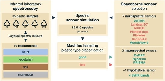
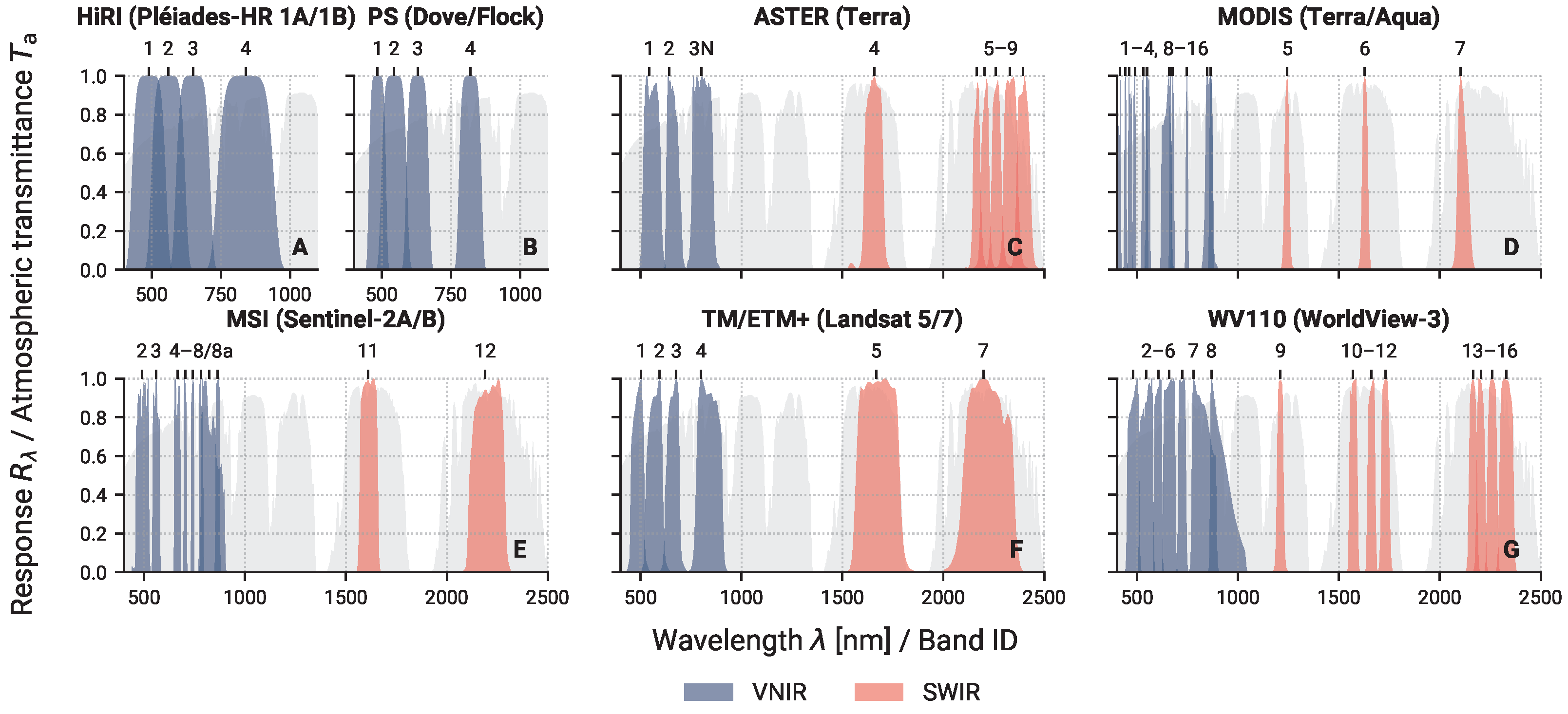
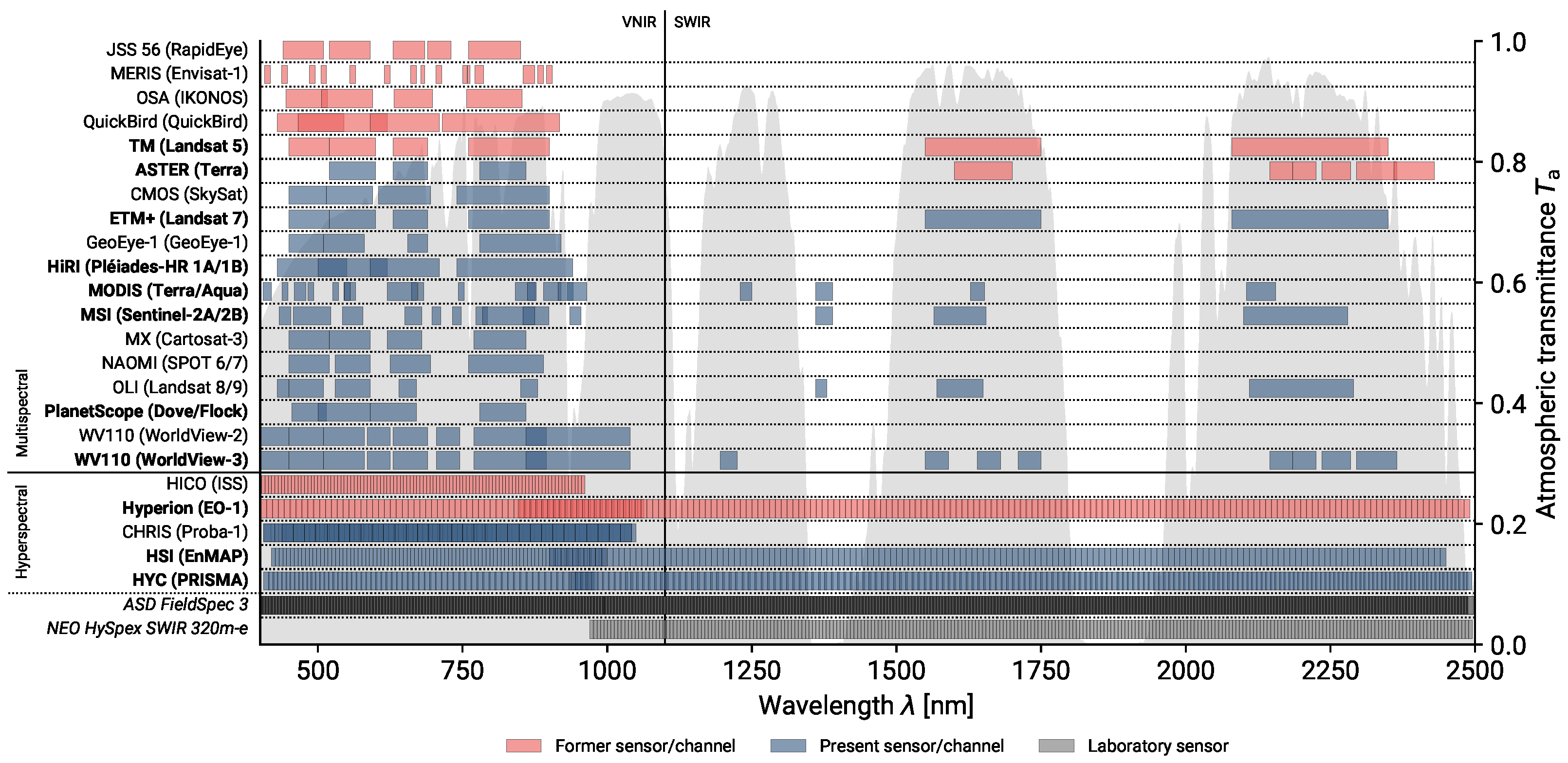
2.1. Spaceborne Sensor Selection

Spectral channel constellations of 22 former and present multi- and hyperspectral optical spaceborne sensors are shown in Figure 1. As some sensors have similar spectral channel configurations or do not have any channels in the SWIR, we made a selection of ten exemplary and representative sensors to use for the spectral sensor simulations. To determine the potential of archive data for estimating spatial and temporal trends of plastics in the environment, we also choose two former sensors (Landsat 5 TM and EO-1 Hyperion). From the present multispectral VNIR sensors, we selected Pléiades-HR 1A/1B HiRI (2011–present, 26 days repeat, 2 m) and Dove/Flock PlanetScope (2014–present, 1 day repeat, 3.5–4 m). From the former and present multispectral sensors that have SWIR channels, too, we choose Terra ASTER (2014–2018, 16 days repeat, 15/30 m), Terra MODIS (1999–present, 1–2 days repeat, 250/500/1000 m), Sentinel-2 MSI (2015–present, 5 days repeat, 10/20 m), Landsat 5 TM/7 ETM+ (1987–2017/2003–present, 17 days repeat, 30 m), and WorldView-3 WV110 (2014–present, <1 days repeat, 1.24/3.7 m). Although the ASTER SWIR channels failed in 2008, we used them for the sensor simulations to determine the potential of the ASTER archive data. Since the channel constellation of Sentinel-2 is very similar to that of Landsat 8/9, but also has more NIR channels, we decided to simulate Sentinel-2. However, the results in the SWIR are also applicable to Landsat 8 and 9. From the former and present hyperspectral sensors, we selected EO-1 Hyperion (2000–2017, ~200 days repeat, 30 m), EnMAP HSI (2022–present, 27 days repeat, 30 m), and PRISMA HYC (2019–present, 29 days repeat, 30 m), as these sensors have bands in the SWIR as well.

2.2. Spectral Database

2.2.1. Plastic Samples

Fifty-three plastic samples of six different types (

Table 1. Plastic types used for the spectral database. In total, we used 53 samples of 6 different types, while we handled PE-HD and PE-LD as one plastic type, i.e., PE.

Acronym	Chemical Notation	Number of Samples
PE-HD	High-density polyethylene	8
PE-LD	Low-density polyethylene	9
PET	Polyethylene terephthalate	8
PP	Polypropylene	12
PS	Polystyrene	8
PVC	Polyvinyl chloride	8

) served as the basis for the spectral database. They were of different color, transmissivity, structure, thickness, cleanness, and degree of weathering (Figure 2). However, a diameter of at least 10 mm had to be guaranteed in order to measure them with an ASD Contact Probe. We took the samples from different sources. Some pristine samples were directly from the factory, while we sampled others from everyday objects and packaging. The six plastic types correspond to those that have been assigned a code of 01–06 as part of the International Resin Identification Coding System (RIC). Thus, they are one of the most commonly used types. For the classifications, we handled PE-HD and PE-LD as one plastic type, i.e., PE. They mostly cannot be distinguished even in laboratory spectroscopy as they comprise the same monomers but differ in their molecular structures, which causes different densities [16,35].

2.2.2. ASD Data Collection

We used an ASD FieldSpec 3 imaging spectrometer for reflectance measurements in the VIS and NIR spectral range (Figure 3). It covers 2151 spectral channels at a wavelength range from 350–2500 nm with full widths at half maximum (FWHM) of 3 nm (350–1000 nm) and 10 nm (1000–2500 nm) and spectral sampling intervals (SSI) of 1.4 nm (350–1000 nm) and 2 nm (1000–2500 nm), which are resampled to 1 nm by the instrument’s operating software [36].

We conducted all measurements in a dark room laboratory. For this, we used an ASD Contact Probe, which is a handheld device. This enabled contact measurements of the plastic samples with the benefit of minimizing noise. A single mean spectrum was calculated from 100 individual spectra for each sample by the internal measuring software, respectively.

For the conversion of the measured radiance to apparent reflectance ($R_{\mathrm{a}}$), we used a SphereOptics Zenith Polymer© PTFE 90% gray reference with a known reflectance spectrum. The experimental setup consisted of measuring each sample on a white and black sponge rubber mat, respectively, while we excluded the absorption bands of the sponge rubber mats. This setting was necessary to extract real reflectance ($R_{\mathrm{r}}$) and transmittance (T) of the measured $R_{\mathrm{a}}$, i.e., the reflectance of the sample and its background (Appendix A.2).

2.2.3. HySpex Data Collection and Processing

Since with the ASD Contact Probe only a single spectrum per sample were possible, we also applied imaging spectroscopy. We used a NEO HySpex SWIR 320m-e imaging spectrometer for reflectance measurements in the SWIR spectral range (Figure 3). It covers 256 spectral channels at a wavelength range from ~970–2500 nm with a FWHM of 7 nm and an SSI of ~6 nm [37].

We carried out the measurements in a dark room laboratory after internal protocol [38]. The spectrometer measured across the movement direction of the stage and averaged eight records per row in order to obtain a higher signal-to-noise ratio (SNR). In this way, images were created from which we gained 50–100 individual spectra from each sample by manually selecting the regions of interest (ROIs). This resulted in a total of 10,182 spectra, which, on average, corresponds to ~192 spectra per sample. We selected the ROIs in areas showing no specular reflections, which are caused by anisotropic reflectance of a material. We again used the SphereOptics Zenith Polymer^© PTFE 90% gray reference to convert the measured radiance to $R_{\mathrm{a}}$. The experimental setup was similar as for the ASD spectrometer in order to allow the calculation of $R_{\mathrm{r}}$ and T (Appendix A.2). However, instead of white sponge rubber mats, we placed white glass fiber filters underneath the samples, which have no absorption bands.

All of the spectra that we picked on the HySpex images were subjected to automated flagging and subsequent cleaning using five conditions, which are described in Appendix A.1. This resulted in a total of 8261 spectra (~156 spectra per sample), which were available for further analysis. Since the signals that we measured with the ASD already correspond to an average spectrum of over 100 spectra through the device, they were not subjected to flagging and cleaning.

Finally, we merged reflectance spectra measured with the ASD spectrometer with those measured with the HySpex imaging spectrometer in order to maximize the number of spectra, while exploiting the total spectral range of 350–2500 nm (Appendix A.3).

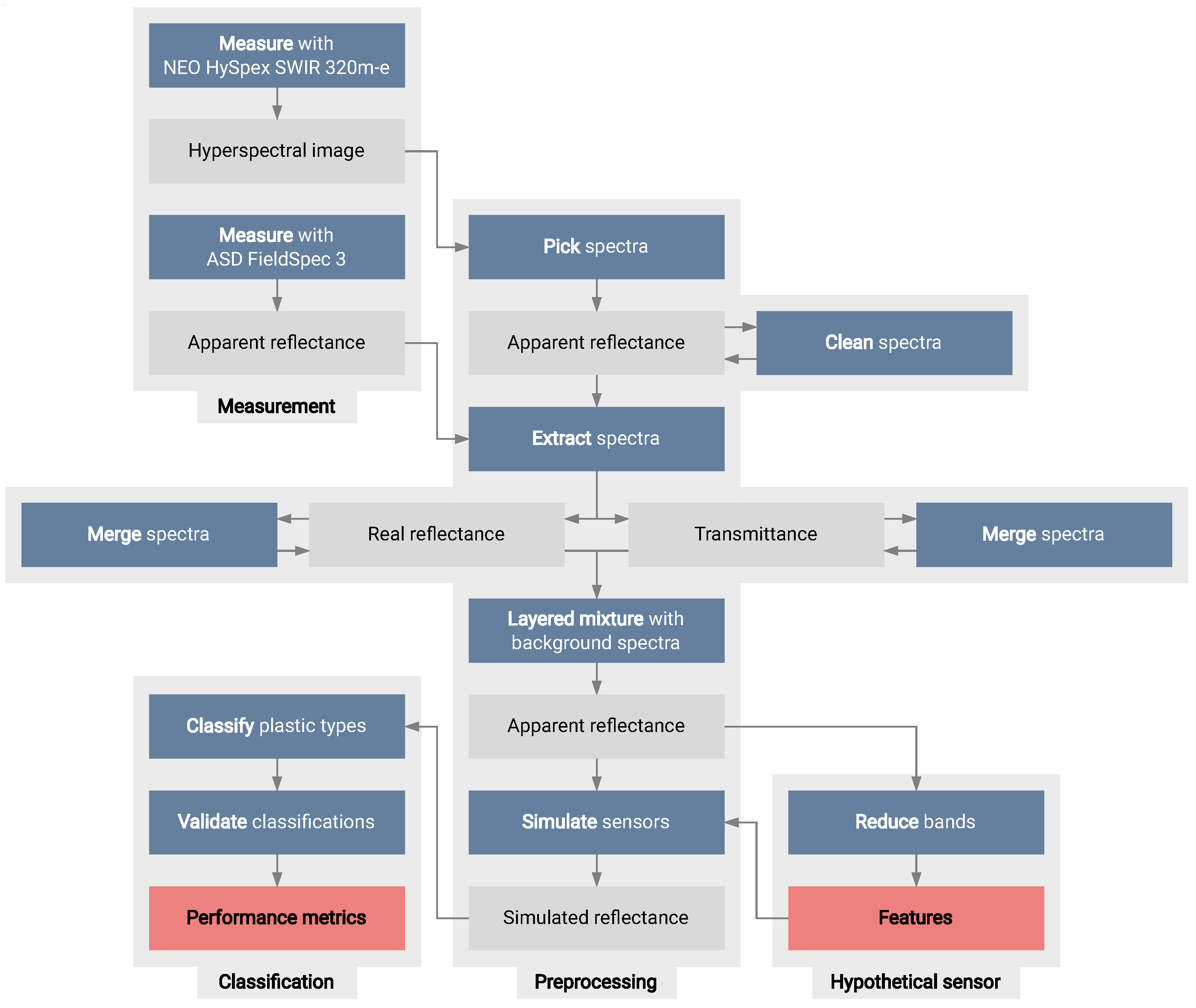
2.3. Spectral Database Processing

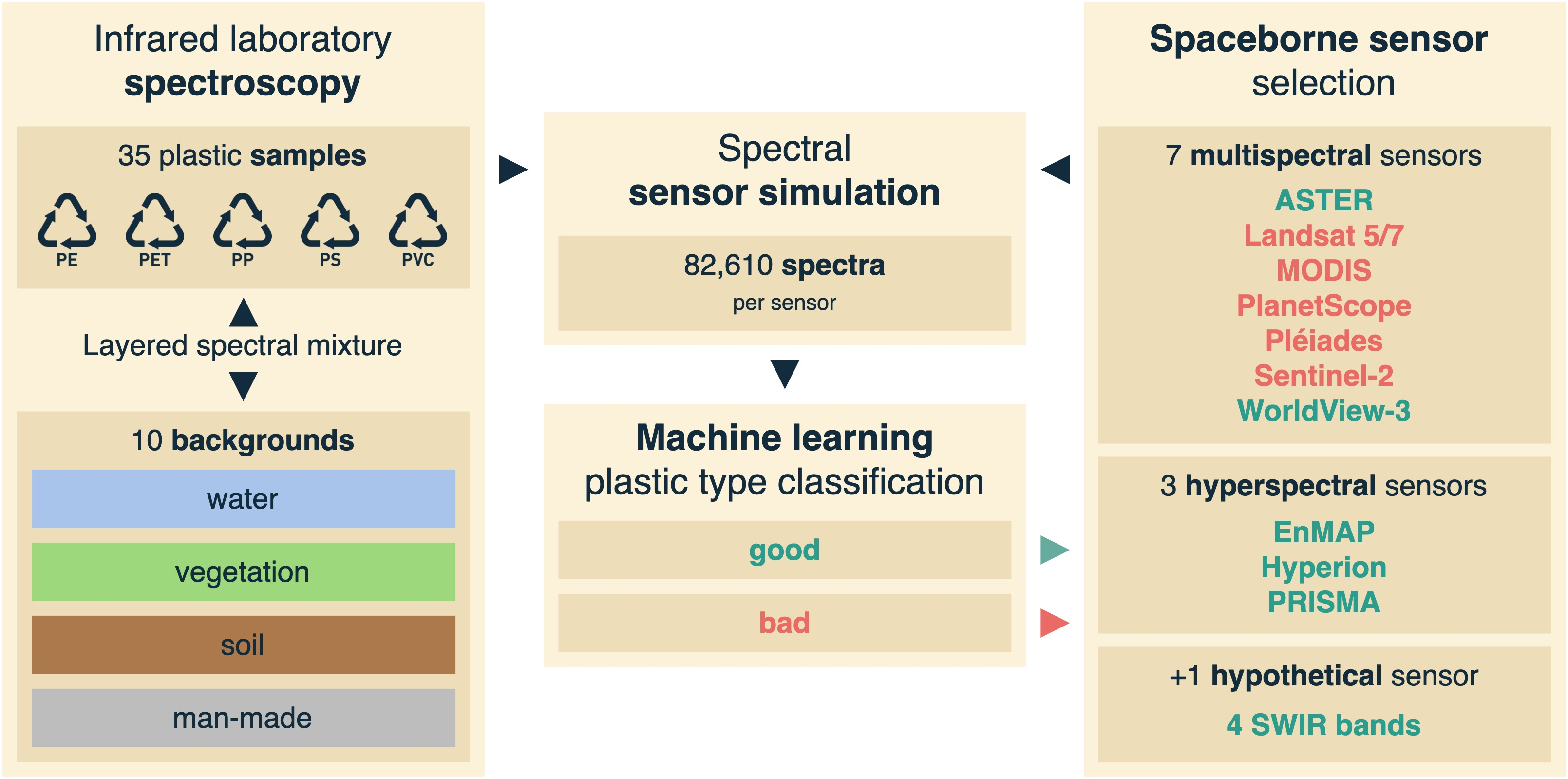
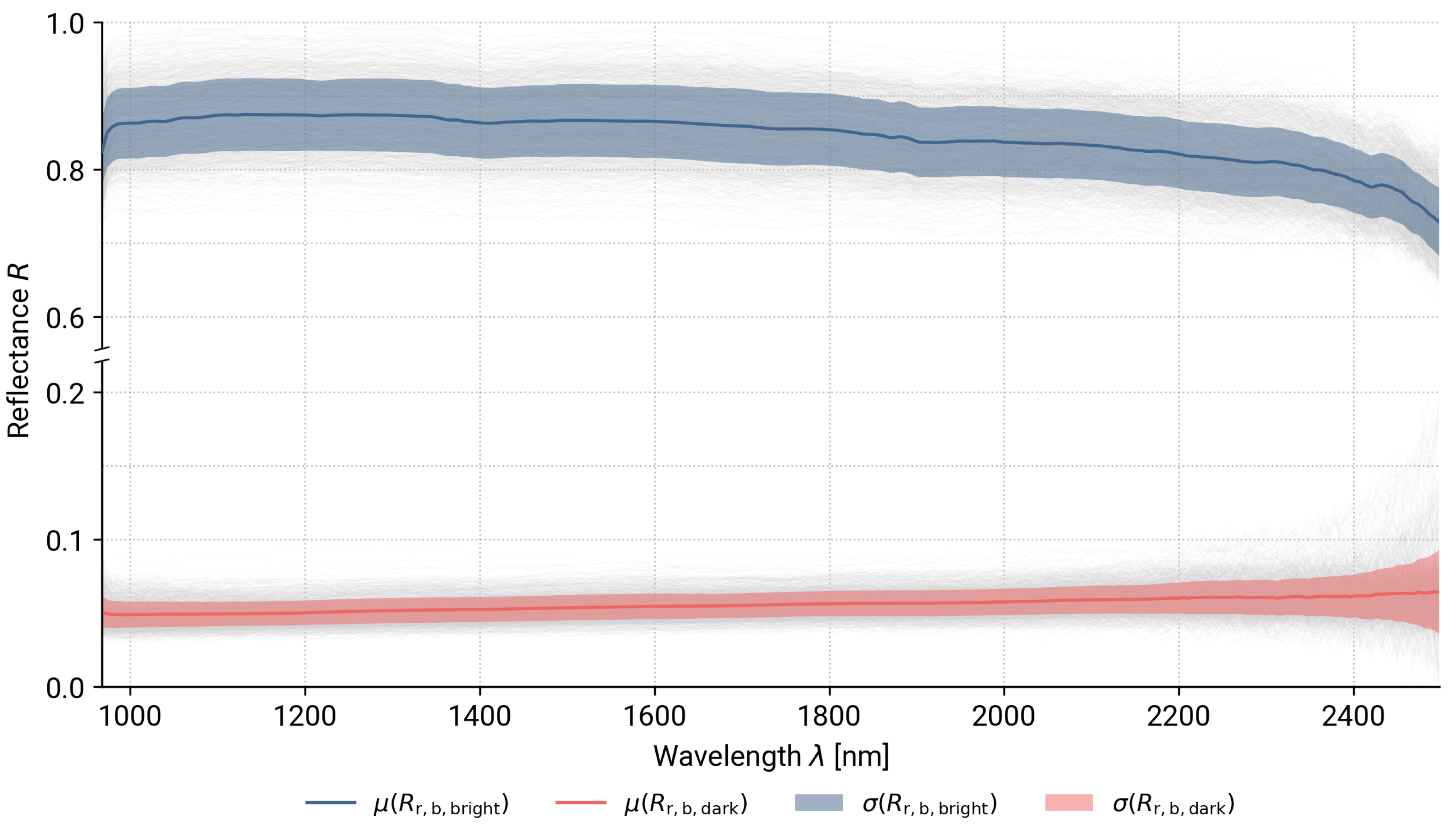
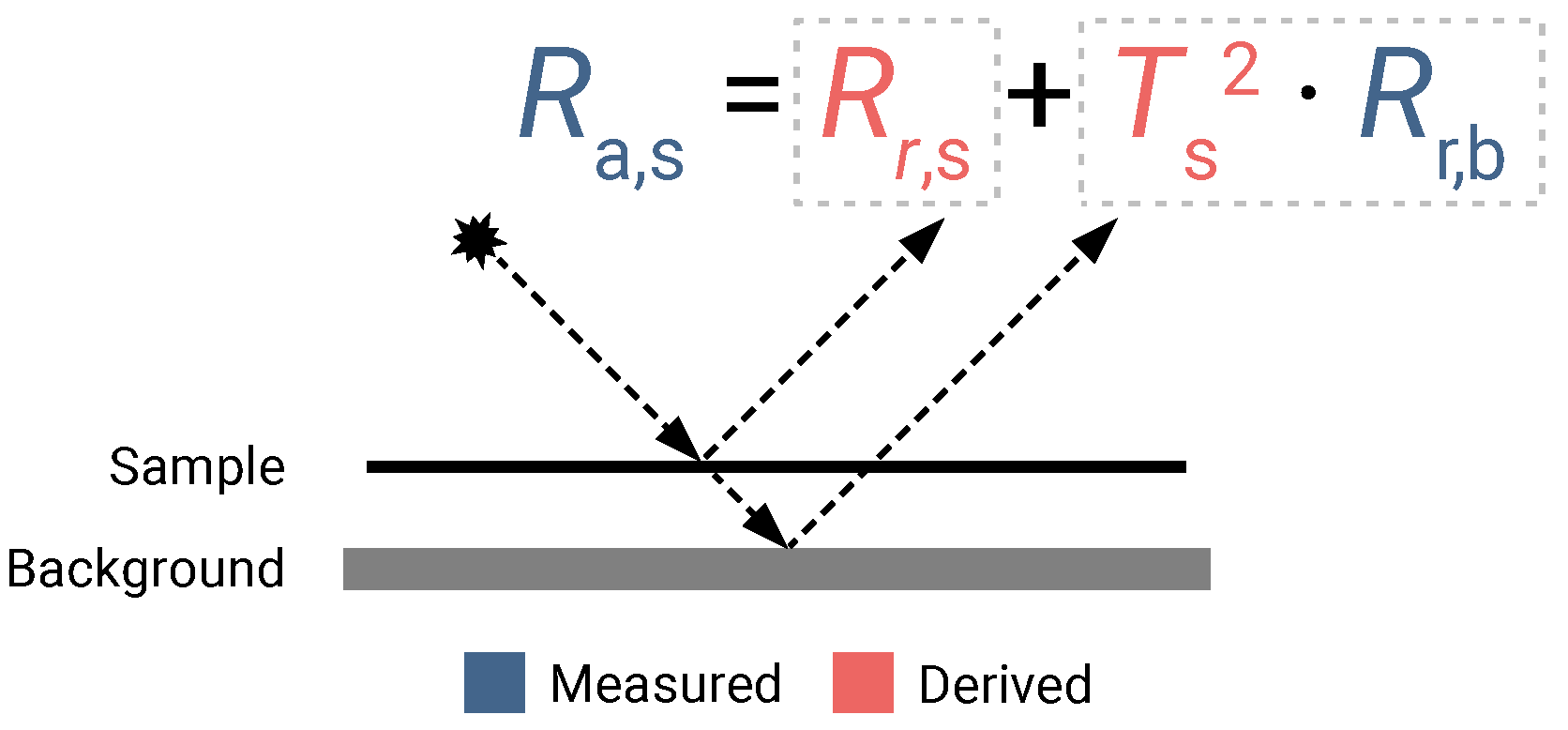
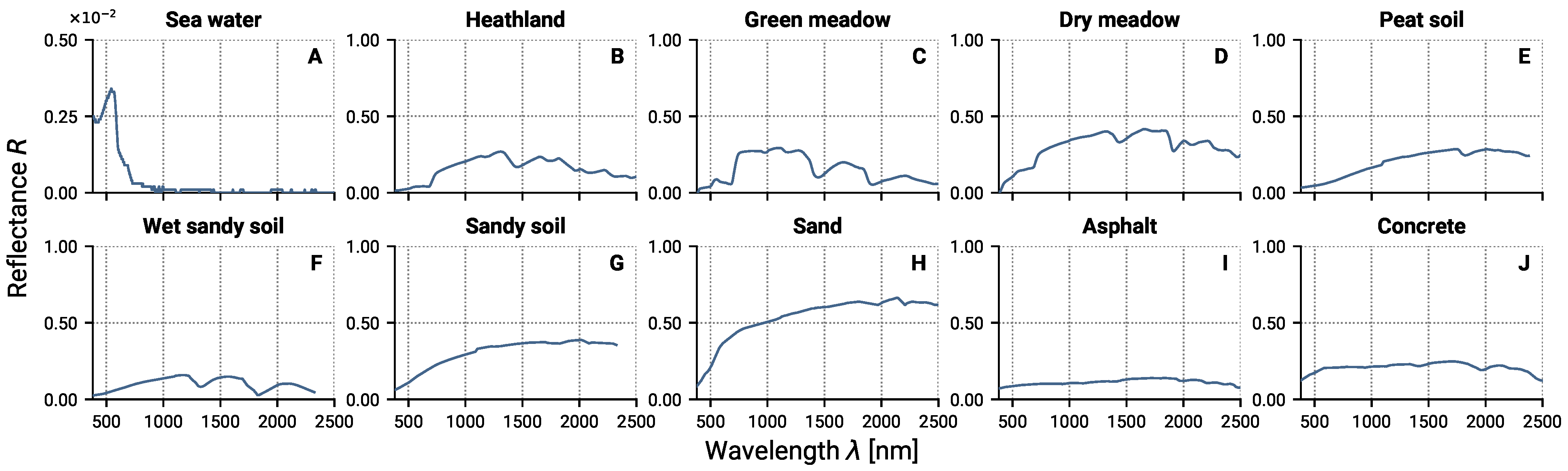
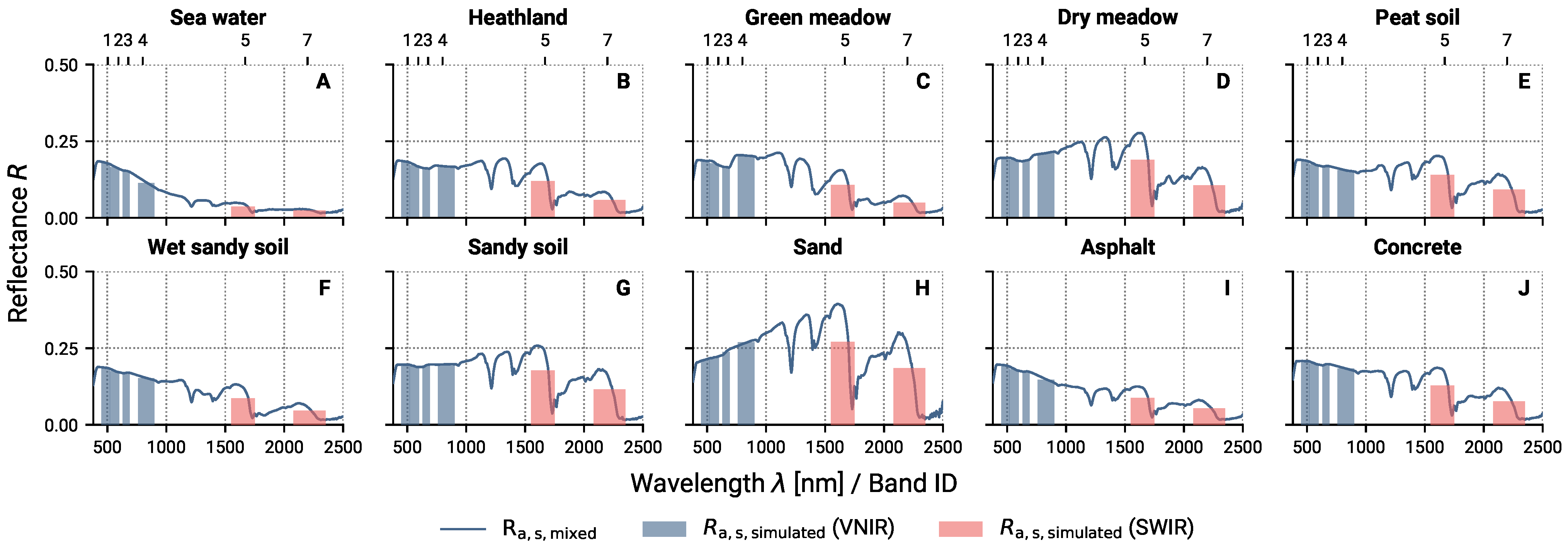
2.3.1. Layered Spectral Mixture with Background Surfaces

Due to the transparency of many plastic samples, it is important to consider background surfaces for the evaluation of sensors to differentiate plastics in the environment. We used reflectance spectra in wavelengths from 350–2500 nm of ten typical land cover types: sea water [39], heathland [40], green meadow [41], dry meadow [41], peat soil [42], wet sandy soil [43], sandy soil [43], sand [40], asphalt [44], and concrete [44], whose spectra are shown in Figure 4. The spectrum of the sea water as the only non-terrestrial surface stands out, as water absorbs nearly all energy in the considered wavelength range. Thus, its spectrum is almost completely zero (Figure 4A). This implies that the plastic sample is directly on the water surface, since a slight sinking would obscure its reflectance.

To obtain the apparent reflectance spectra, $R_{\mathrm{a},\mathrm{s}}$, of plastic samples as they would appear on the different environmental surfaces, we applied a layered spectral mixture, weighted by the square of the plastic sample transmissivity, $T_{\mathrm{s}}$, as follows:

$$R_{\mathrm{a},\mathrm{s}}=R_{\mathrm{r},\mathrm{s}}+T_{\mathrm{s}}^2·R_{\mathrm{r},\mathrm{b}},$$

(1)

where $R_{\mathrm{r},\mathrm{s}}$ is the real reflectance of the plastic sample and $R_{\mathrm{r},\mathrm{b}}$ is the real reflectance of the background.

This allowed for the increase of the number of $R_{\mathrm{a},\mathrm{s}}$ spectra by a factor of ten, which is particularly useful for plastic types with few spectra. For each sensor and background, a total of 8261 spectra were then available. Beforehand, we resampled the discrete environmental surface spectra to match the wavelengths of the laboratory plastic measurements. Both sandy soil surfaces (Figure 4F,G) were measured up to 2450 nm only. However, since simulated multispectral sensors have no spectral channels in wavelengths above 2450 nm, we retained them.

2.3.2. Spectral Sensor Simulation

We used the apparent reflectance spectra of the plastic samples on the different background surfaces to carry out the spectral sensor simulation (Figure 5). There are many steps involved in an end-to-end sensor simulation that comprises a forward and a backward simulation [45,46]. The forward simulation involves the spectral resampling, to which we limited the simulation in the scope of this study. This facilitates the comparison of different spectral specifications despite spatial limitations (see also Section 4.3).

Spectral resampling requires the sensor’s spectral response functions (SRF), which comprise the spectral response per channel ($R_{\lambda }$) at discrete wavelengths. Typically, SRFs are measured under laboratory conditions [47] but can also be modeled. In this case, $R_{\lambda }$ is defined as follows [46]:

$$R_{\lambda }\left(\lambda \right)=\left\{\begin{array}{cc}{\mathit{e}}^{-2{\left(\frac{\sqrt[2]{\ln 4}(\lambda -{\lambda }_c)}{\Delta \lambda }\right)}^2}\hfill & \mathrm{if}\Delta \lambda <10\mathrm{nm},\hfill \\ {\mathit{e}}^{-32{\left(\frac{\sqrt[6]{\ln 4}(\lambda -{\lambda }_c)}{\Delta \lambda }\right)}^6}\hfill & \mathrm{otherwise},\hfill \end{array}\right.$$

(2)

where $\lambda$ is the wavelength at which $R_{\lambda }$ is calculated, ${\lambda }_{\mathrm{c}}$ is the central wavelength of the channel, and $\Delta \lambda$ is the bandwidth, i.e., full width at half maximum (FWHM). As shown in Equation (2), the response of narrow channels, i.e., $\Delta \lambda <10\mathrm{nm}$, can be approximated with a normal distribution, whereas that of broader channels, i.e., $\Delta \lambda \ge 10\mathrm{nm}$, with a modified normal distribution [45]. We computed the SRFs of Pléiades (Figure A3A), PlanetScope (Figure A3B), EnMAP, Hyperion, and PRISMA, for which no SRFs have been published. For the remaining sensors, we used the published SRFs.

We did not use cirrus and water vapor channels for simulations, because of their ability to measure atmospheric phenomena only. This reduced the number of simulated channels from MODIS, Sentinel-2, and WorldView-3 compared to their total number of channels. The channels selected for the simulations are found in Appendix B.1.

We also added noise to the simulated reflectance signals to investigate the influences of hypothetical signal-to-noise ratios (SNRs) or atmospheric noise on the classification performances. Since published SNRs are valid for radiance data, we did not use them to compute the noise, as it would suggest a wrong accuracy. Instead, we added random Gaussian noise with a mean of 0 and a standard deviation of 0.05 to the simulated signals. We fixed a random seed and the noise arrays for the classifications using both k-NN and RF to ensure the same data for all simulations. If the noise addition resulted in negative values or in values above 1, we set the reflectance to 0 or 1, respectively. Afterwards, we applied a one-dimensional Gaussian filter with a kernel standard deviation of 0.06. This created more realistic data, as reducing noise before classifications is a common pre-processing step.

2.3.3. Continuum Removal

We applied a continuum removal, adapted after Mielke et al. [48], to the simulated reflectance spectra of hyperspectral sensors in order to normalize the spectra by their continuum so that the absorption bands are emphasized and comparable regardless of the albedo of the sample [49]. Finally, we masked the simulated reflectance spectra of the hyperspectral sensors at wavelength ranges of water absorption bands, i.e., 1350–1410 nm and 1815–1935 nm [34]. This ensured comparable classification performances between multispectral and hyperspectral sensors, as the former do not have channels in these wavelength ranges, except for cirrus or water vapor channels, which we did not simulate.

2.4. Classification

2.4.1. Classifiers

The higher accuracies of machine learning classifiers compared to traditional parametric classifiers for applications in remote sensing are found in many studies [50]. We classified the plastic types of simulated reflectance signals using two probabilistic supervised machine learning classifiers: the non-ensemble method k-nearest neighbor (k-NN) and the ensemble method random forest (RF). Unlike other classifiers, k-NN does not train a model but uses the entire training set as a reference for classification [50,51]. RF uses an ensemble of decision trees to make predictions [52]. We applied two different classifiers to compare their performances against each other using the identical spectral database. To optimize the performance of the classifiers, we used exhaustive grid search to tune their parameters, as outlined in Appendix C.1. The degrees of freedom for the classifications were plastic type, background surface, sensor, and noise.

2.4.2. Performance Metrics

To validate the classifications, we employed an 8-fold cross-validation using equalized stratified random sampling, resulting in various confusion matrices (see Appendix C.2). Class-based evaluation is essential for multi-class classifications, as performance differences can arise between classes. We calculated precision, recall, F1 score, and macro F1 score from the respective confusion matrices.

2.4.3. Case Study Almería

To assess the applicability of the classifiers trained with the simulated signals on actual remote sensing data, we selected a case study on plastic roofs of greenhouses in Almería, southeast Spain. These greenhouses were built in large numbers since 1960 and offer a suitable environment for a case study. To date, the area of greenhouses has expanded to almost 500 km² in this region, while new greenhouses continue to be built. On satellite imagery, they can be well detected, as their white-appearing roofs are very clearly visible in the dry and sparsely populated region (Figure 6). With a few exceptions, their roofs and walls are made of transparent PE films [53]. This enables the classifiers to be tested since the true positive is known in advance.

We used satellite imagery of a part of Almería captured with PRISMA on 24 June 2020 and with Sentinel-2 on 29 June 2020 to determine the plastic types of the greenhouse roofs. As the classifiers can only differentiate between the five selected plastics, we masked the greenhouses on both images in advance using a deterministic albedo threshold approach. As the greenhouses appear white in the VIS, we set an albedo of 0.20 (PRISMA) and 0.25 (Sentinel-2) in the VIS as the threshold for identification. For these masked areas, we applied k-NN and RF as trained using the respective simulated signals to differentiate between the plastic types.

2.5. Hypothetical Sensor Definition

We proposed a hypothetical sensor with an optimal spectral channel constellation for the differentiation of plastics in the environment. For this, we performed a forward greedy selection using the k-nearest neighbor (k-NN) classifier. To select individual spectra per plastic type, we used equalized stratified random sampling. Input spectra for the forward greedy selection were continuum-removed apparent reflectance spectra on all background surfaces, masked at wavelength ranges of water absorption channels. As the distinctive absorption channels of plastics are in SWIR, we only selected the wavelength range from 1100–2500 nm. From the remaining 959-dimensional feature space, we selected ten subsets of features, while each subsequent set contains the features of the previous set. We later used these features as the central wavelengths of the hypothetical sensor for classifications. Using different FWHMs (10, 15, 20, 50, and 100 nm), we classified all feature sets with k-NN and RF, respectively. We finally suggested the central wavelengths–FWHM combination with the highest mean macro F1 score as the ideal hypothetical sensor.

3. Results

3.1. Classification

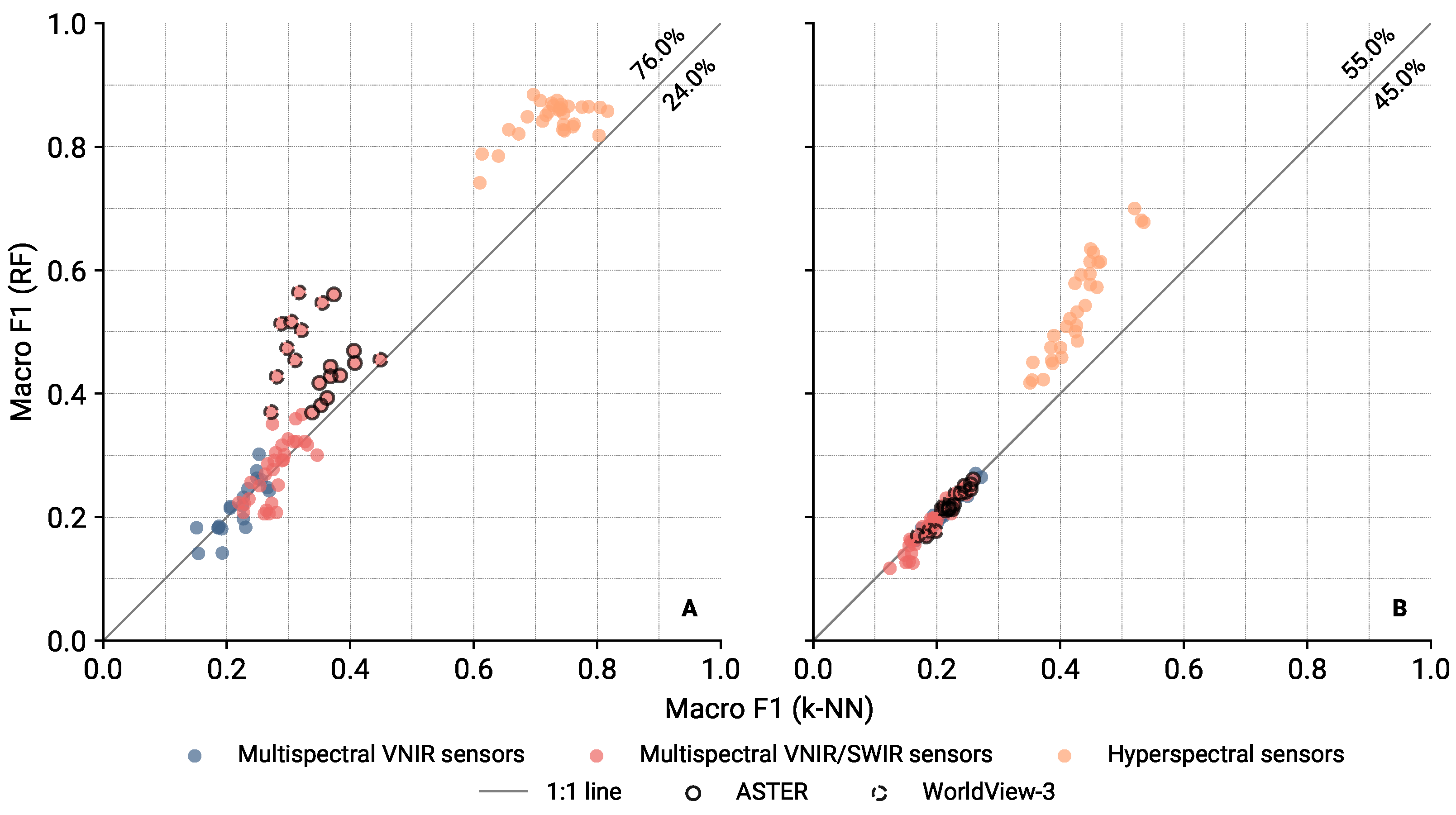
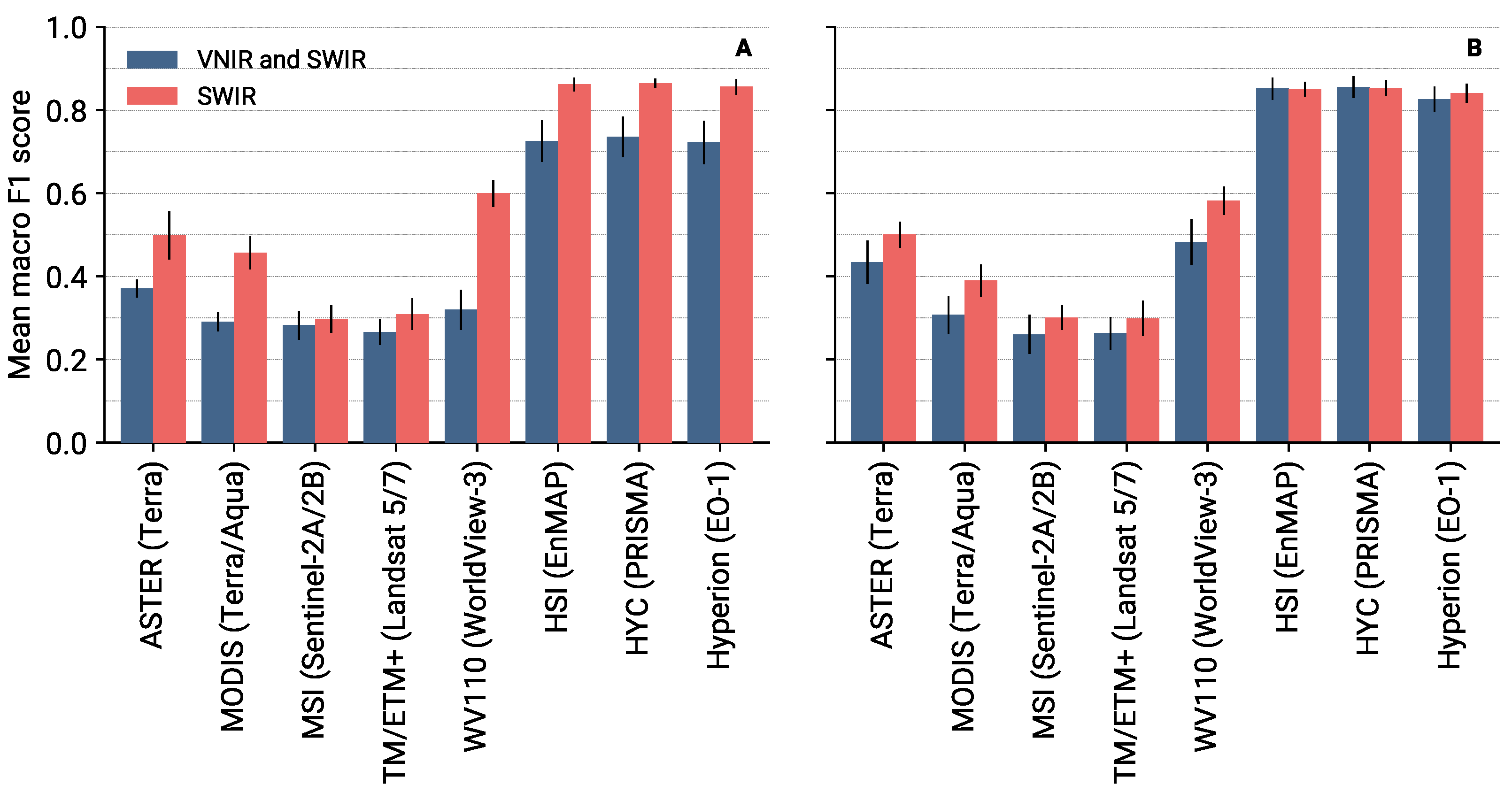
3.1.1. Macro F1 Scores: Influence of Sensor, Background, and Noise

In order to initially compare the performance of the two classifiers on a large scale, the variability of the macro F1 scores that were achieved using all sensors on all background surfaces are shown in Figure 7, while simulated signals without and with 5% noise are considered separately.

The results using RF were generally higher than using k-NN. For simulated signals to which no noise was added, this was true for 76.0% of all cases. In particular, for sensors whose macro F1 scores were relatively high, i.e., ASTER, WorldView-3, and the hyperspectral sensors, the difference between the two classifiers was greatest, while RF consistently achieved higher scores. For signals of multispectral VNIR sensors and multispectral VNIR/SWIR sensors (except ASTER and WorldView-3), the classification results with both classifiers were very similar. For simulated signals to which 5% noise was added, the classification performances using multispectral sensors had very small deviations between both classifiers and were in the same range, regardless of whether they belonged to the VNIR or the VNIR/SWIR sensors. For the latter, the macro F1 scores were significantly lower than using signals without noise. The variability of the macro F1 scores using signals of multispectral sensors with noise was significantly lower than without noise. ASTER and WorldView-3 also no longer stood out. Only the signals of the hyperspectral sensors could be reliably classified even with noise, despite lower macro F1 scores, while RF surpassed k-NN. The variability of the score between both classifiers was similar, and thus their accuracies. The opposite partly applies to their precisions, which were similar for multispectral VNIR sensors, but slightly different for multispectral VNIR/SWIR, and even greater for hyperspectral sensors, so that RF had a higher precision, i.e., higher macro F1 scores were generally achieved. Due to this, the results are evaluated in the following with this classifier as they reflect more robust trends, unless outstanding results obtained with k-NN are noteworthy.

Regardless of the similarities and differences in the performance of the two classifiers, clear differences can be identified between the sensor types in terms of their potential to differentiate plastics. This can also be seen in the context of the differentiated consideration of the macro F1 score per sensor and background surface using noise-free signals classified with RF (Figure 8). Multispectral VNIR sensors (Pléiades and PlanetScope) output the lowest mean macro F1 scores compared to other sensor types, as could already be deduced from Figure 7. The scores achieved with the signals of this sensor type had very similar means and standard deviations, i.e., $0.21\pm 0.05$ (Pléiades) and $0.22\pm 0.03$ (PlanetScope), but different ranges, i.e., 0.14–0.30 (Pléiades) and 0.18–0.27 (PlanetScope) (Figure 8A). These low scores were not better than random classification, i.e., 0.2 (using five classes), and are the logical consequence of plastics having no diagnostic absorption bands up to ~900 nm (see also Figure 9).

The results using signals of multispectral VNIR/SWIR sensors showed greater variability and, as was mentioned above, can be split into two clusters, i.e., MODIS, Sentinel-2, and Landsat 5/7 and ASTER and WorldView-3 (Figure 8B). Macro F1 scores achieved with sensors of the first cluster were in the range from 0.21 to 0.37, with means and standard deviations of $0.31\pm 0.05$ (MODIS), $0.26\pm 0.05$ (Sentinel-2), and $0.26\pm 0.04$ (Landsat 5/7). Thus, they were either in the same range of the scores achieved with multispectral VNIR sensors or insignificantly higher. In contrast, the scores achieved with ASTER and WorldView-3 were the highest values among this sensor category, while both ranged from 0.37 to 0.56 but had different means and standard deviations, i.e., $0.43\pm 0.05$ (ASTER) and $0.48\pm 0.06$ (WorldView-3).

Classifications using continuum-removed signals of all hyperspectral sensors were most successful, which is reflected in their relatively high mean macro F1 scores, which were $0.83\pm 0.03$ (Hyperion), $0.85\pm 0.03$ (EnMAP), and $0.86\pm 0.03$ (PRISMA) (Figure 8C). In contrast, when classifying simulated reflectance signals of the hyperspectral sensors, without removing their continua in advance, mean macro F1 scores of $0.49\pm 0.03$ (Hyperion), $0.51\pm 0.04$ (EnMAP), and $0.50\pm 0.03$ (PRISMA) were obtained. These scores were thus in the range of those of WorldView-3 and therefore did not stand out compared to this multispectral sensor. However, after continuum removal, as is often done with hyperspectral data, the results stood out. This suggests that a classification of plastics with hyperspectral sensors can achieve the best results among all selected types of sensors, as they scan the spectral range in which are the diagnostic absorption bands of plastics with a sufficiently high spectral resolution.

Mean macro F1 scores among the background surfaces were very similar and ranged from 0.43 (sand) to 0.50 (heathland). This indicates that the sensors performed with a relatively consistent performance across the various surfaces. While variations in macro F1 scores were observed between sensors on specific surfaces, no single background surface was found to consistently yield exceptional classification results across all sensors. Therefore, the modest differences in macro F1 scores between backgrounds were not statistically significant and unlikely to be of practical consequence.

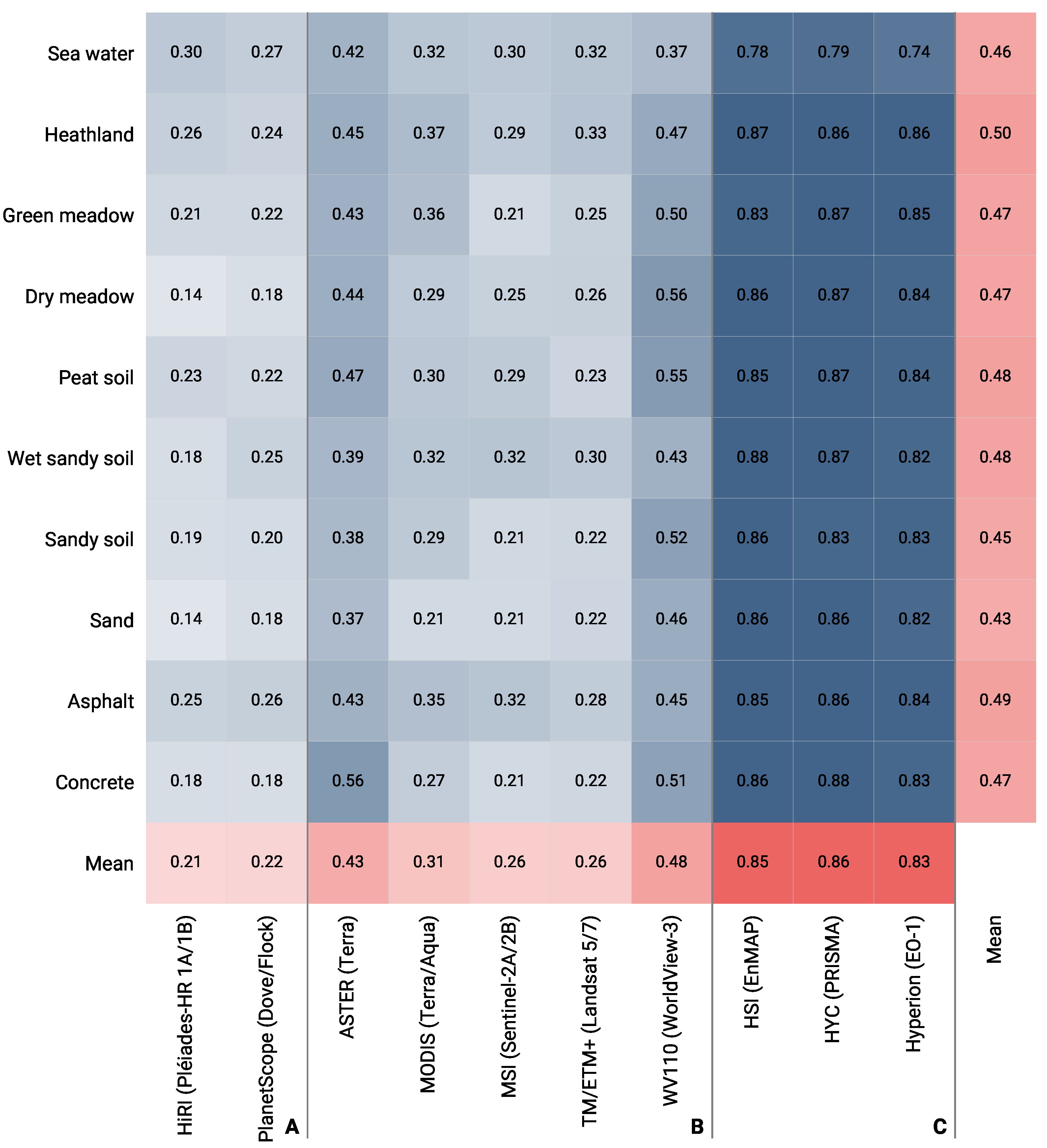
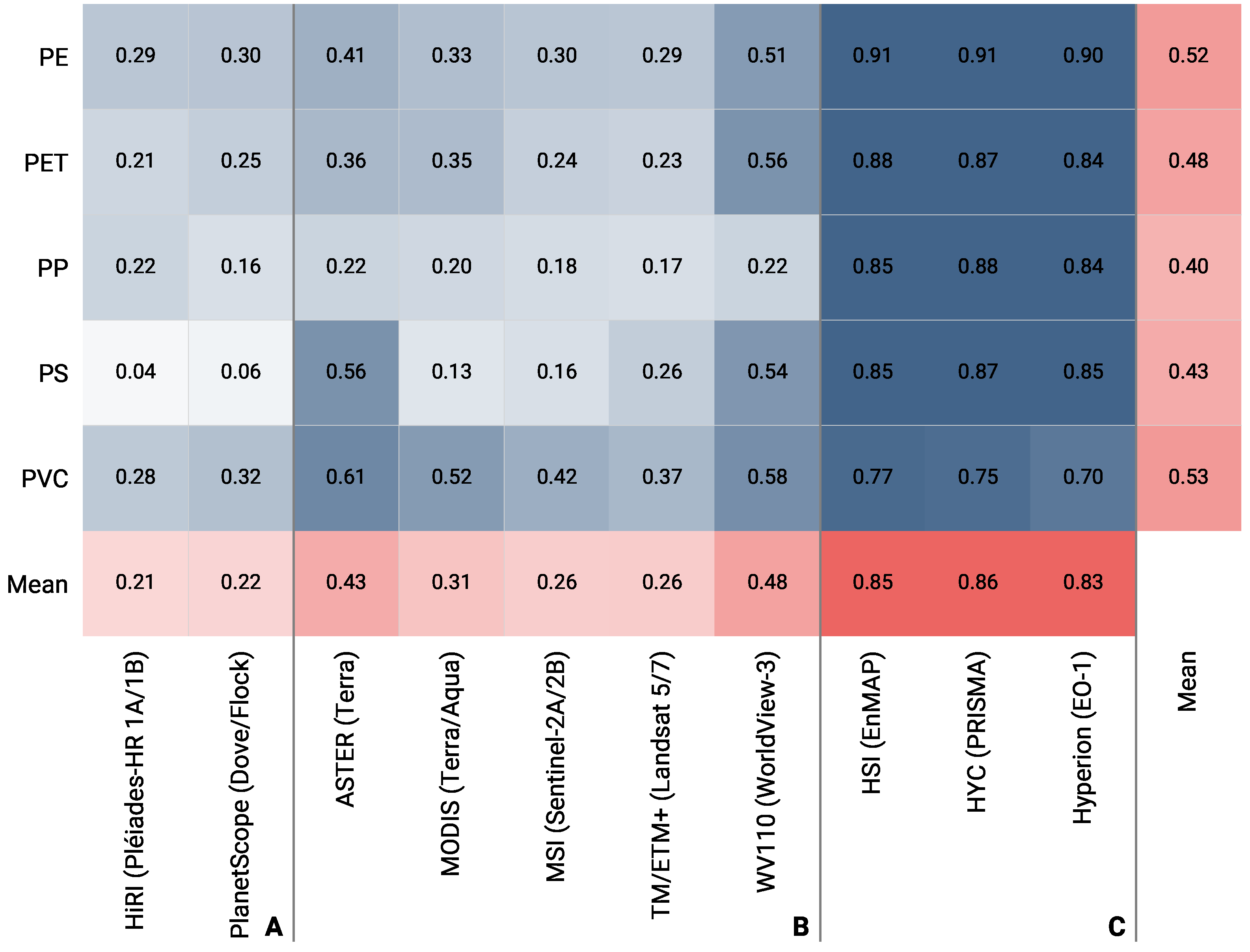
3.1.2. F1 Scores: Influence of Plastic Type

Differences among sensor types are also evident when considering performances per plastic type, quantified by the mean F1 scores over all background surfaces per sensor (Figure 10). In contrast to the background surfaces (see paragraph above), there was a greater variability between plastic types, such that the mean F1 scores range from $0.40\pm 0.30$ (PP) to $0.53\pm 0.17$ (PVC).

The greatest differences between the individual plastic types can be found in the analysis of the individual sensor types. The classification of PS generally had the broadest range, and the signals of multispectral VNIR sensors resulted in very low scores, i.e., 0.04 (Pléiades) and 0.06 (PlanetScope), which were markedly below the mean scores of both sensors, i.e., $0.21\pm 0.05$ (Pléiades) and $0.22\pm 0.03$ (PlanetScope) (Figure 10A). These very low values also stand in contrast to all other plastic types, with achieved value ranges from 0.21 (PET) to 0.29 (PE) using simulated Pléiades signals and 0.16 (PP) to 0.32 (PVC) using simulated PlanetScope signals.

The relatively low mean F1 score of PP achieved with PlanetScope was part of the trend within the multispectral VNIR/SWIR sensors, as this plastic type had the lowest mean F1 score on average within this group (Figure 10B). This trend was evident for all classification results of signals of multispectral VNIR/SWIR sensors, regardless of the better classification results that were generally achieved with ASTER and WorldView-3. For the remaining plastic types, the better classifiability with both sensors was applicable, whereby the highest mean F1 scores were achieved with PVC, i.e., 0.61 (ASTER) and 0.58 (WorldView-3). These values stand out especially for signals of ASTER since its mean F1 score was in the range of 0.36–0.61, which was achieved for plastic types different from PP. For signals of WorldView-3, this range was not as broad (0.51–0.58). Among the other sensors in this category, PVC was also consistently best classified, with mean F1 scores of 0.52 (MODIS), 0.42 (Sentinel-2), and 0.37 (Landsat 5/7). As the lowest mean score among these three sensors, PS—as classified using MODIS signals—stands out again (0.13), which could already be classified very poorly with multispectral VNIR sensors.

The observations described for classifications with signals of multispectral sensors were not evident for those from hyperspectral sensors (Figure 10C). On the one hand, the variabilities between the plastic types with hyperspectral sensors were not as high since the mean F1 score ranges 0.70–0.90 (Hyperion), 0.75–0.91 (PRISMA), and 0.77–0.91 (EnMAP) were achieved. On the other hand, the lowest and most different mean F1 scores were for PVC, despite the highest mean F1 score of PVC over all sensors.

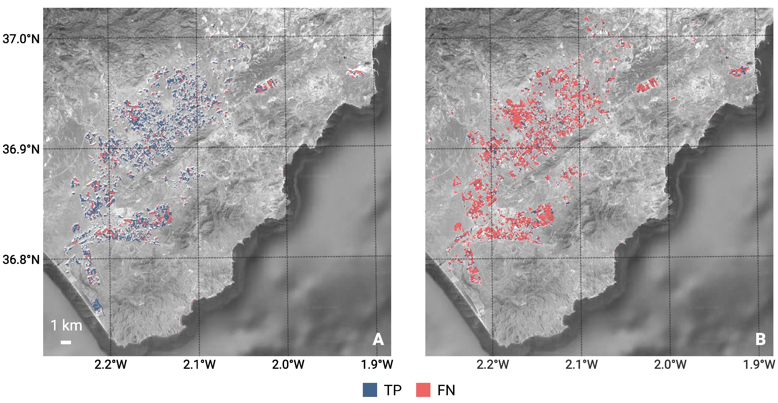
3.1.3. Case Study Almería

Assuming that all greenhouse roofs are made of PE [53], a recall of 0.74 using PRISMA (Figure 11A) and 0.22 using Sentinel-2 (Figure 11B) was obtained as classified with RF, respectively. As no other classes are to be expected, the precision is 1. Thus, the recall equals the macro F1 score, which, on average, were $0.86\pm 0.03$ using simulated PRISMA signals and $0.26\pm 0.05$ using simulated Sentinel-2 signals. Although the performance with the simulated data was slightly better for PRISMA, the result using the hyperspectral image of Almería was very good and reflected the high potential of hyperspectral sensors for the differentiation of plastics. The low performance using the Sentinel-2 image confirms that there is no potential for plastic differentiation using multispectral VNIR/SWIR sensors that have only a few broad SWIR channels.

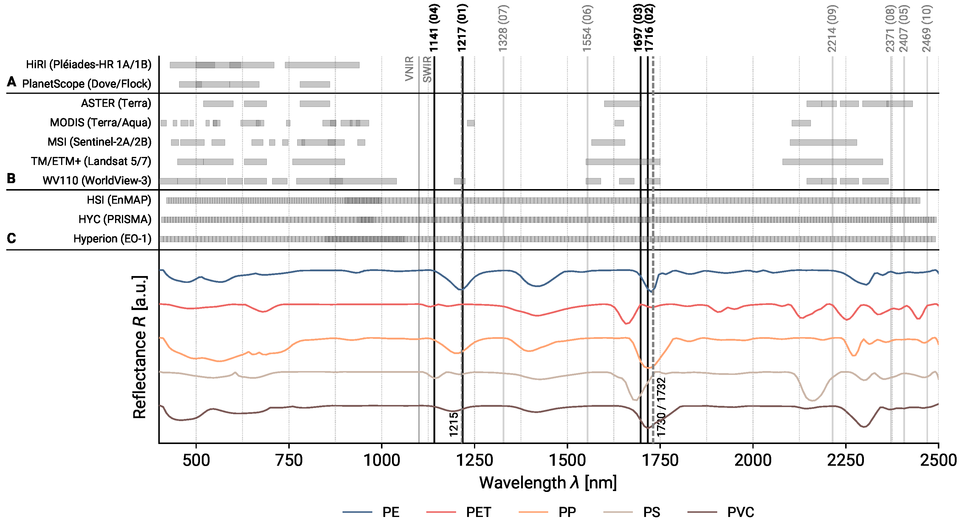
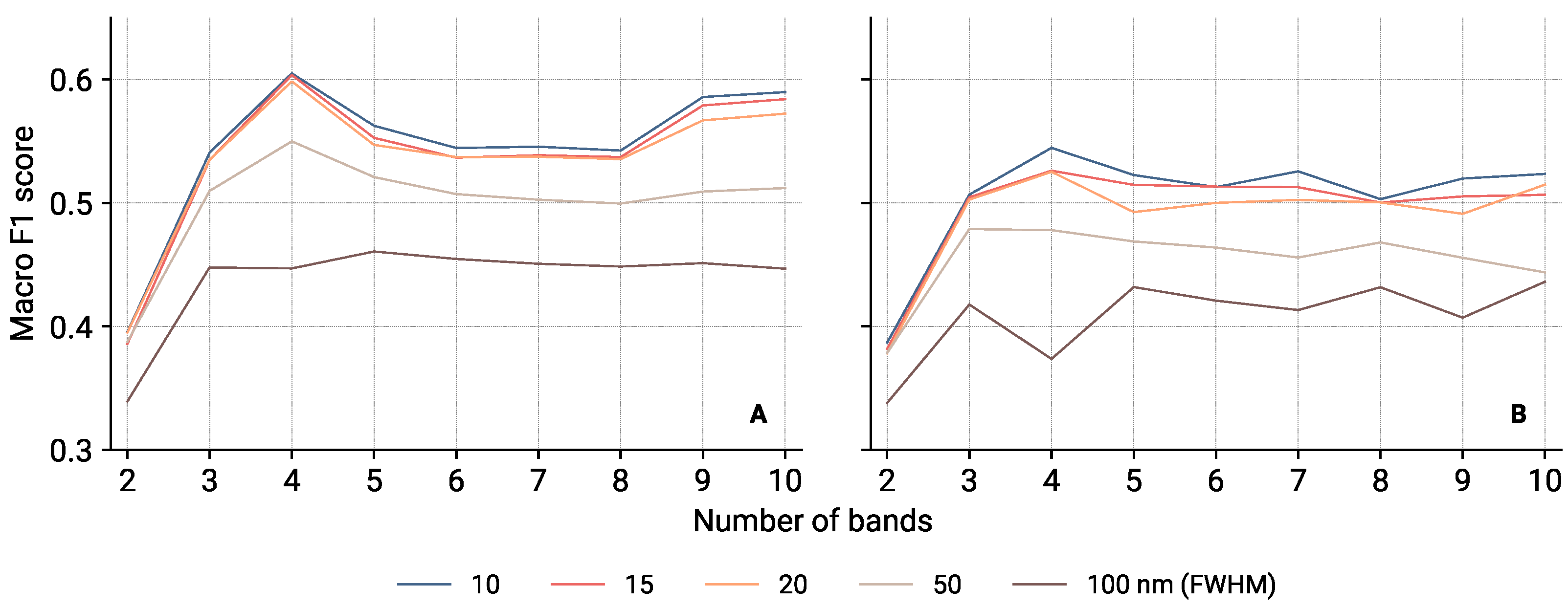
3.2. Hypothetical Sensor Definition

The dimensional reduction of the feature space has many benefits. The sequential greedy forward selection in the SWIR was limited to ten features, which are shown in Figure 9. The first two features were at 1217 and 1716 nm and were very close to the plastic features at 1215 and 1732 nm published by Martínez-Vicente et al. [29] and to the hydrocarbon feature at 1730 nm published by Kühn et al. [21]. Additionally, both selected features are in the wavelength range of two channels of WorldView-3, while the first is in the wavelength range of the channels with the lowest central wavelength in the SWIR among all selected multispectral VNIR/SWIR sensors. The third feature at 1697 nm also matches most absorption bands of the plastic types indicative for the features published by Kühn et al. [21] and Martínez-Vicente et al. [29]. The fourth feature at 1141 nm is located at the shoulder of the absorption bands with the lowest wavelength positions in the SWIR. Feature five at 2407 nm is very close to the central wavelength of ASTER’s channel 9 at 2395 nm, which is the channel with the highest central wavelength among the selected multispectral VNIR/SWIR sensors. The following three features at 1554, 1328, and 2371 nm did not match any absorption bands of the mean plastic spectra but might be crucial for differentiating between certain samples. The ninth feature at 2214 nm is located again at the shoulder of absorption bands and matches with channels of ASTER, Landsat 5/7, Sentinel-2, and WorldView-3. The last feature at 2469 nm was very close to the maximum wavelength of the measured signals and did not match any channel of the selected multispectral VNIR/SWIR sensors, as the atmospheric transmittance at this wavelength is very low.

The first four features (at 1141, 1217, 1697, and 1716 nm) performed best among all feature sets, while a narrower FWHM increases the macro F1 scores (Figure 12). This is evident for all sets of features, while the narrower the channels are, the better the performances are. The macro F1 score was higher than using WorldView-3 signals ($0.48\pm 0.06$) while the number of SWIR channels was lower (four SWIR channels) than that of WorldView-3 (eight SWIR channels). As absorption bands of plastics are narrow too, they can best be measured using narrow channels. An increase in the number of channels, i.e., more than four, does not improve the potential of the hypothetical sensor to differentiate plastics. The performance using k-NN (Figure 12A) is generally better than using RF (Figure 12B). This can be attributed to the choice of k-NN as the classifier for the sequential greedy forward selection. However, as the general trends obtained with both classifiers are similar, with the four features having the highest scores and the correlation of FWHM and score, another run with RF was not completed.

4. Discussion

4.1. Channel Characteristics

The characteristic absorption bands in the SWIR of reflectance spectra of plastics are essential for their differentiation. This was already conducted successfully using laboratory infrared spectroscopy [54], airborne [55], and spaceborne remote sensing [31]. The spectra of some plastics have absorption bands in the NIR (Figure 9). However, there is usually only a single absorption band, which is of shallower depth than absorption bands in the SWIR. In the VIS, in turn, only the color of the plastic can be measured. A classification using VNIR sensors can thus be affected by a color bias, i.e., a distortion of the classification results by the colors of the samples.

Figure 9 shows the spectral channels of the selected sensors and the continuum-removed mean spectra of the selected plastic types. Multispectral VNIR sensors typically only have one NIR channel, as do the selected Pléiades and PlanetScope. Since the reflectance signals in VIS do not contain any information on the plastic type, it cannot be identified with a single NIR channel. Pléiades and PlanetScope mainly differ in the FWHM of their channels, while their central wavelengths show only minor deviations. Pléiades has the broadest NIR channel with 200 nm among a large selection of multispectral VNIR sensors (Figure 1), while PlanetScope has an 80 nm narrow NIR channel. The VIS channels also differ between the two in that Pléiades has broad and relatively strongly overlapping channels and PlanetScope has relatively narrow ones. These differences do not affect the performance of the classification of their signals, though small FWHM potentially increase the classification performance as obtained from the feature selection. By the use of noise-free signals classified with RF mean macro F1 scores of $0.21\pm 0.05$ (Pléiades) and $0.22\pm 0.03$ (PlanetScope) have been obtained. Given five classes (PE, PET, PP, PS, and PVC), the accuracy of correctly classifying a class using random choice would be 0.2. Thus, the classification results using signals of multispectral VNIR sensors are not better than a random classification, which was expected since plastics have no diagnostic absorption bands up to ~900 nm.

Multispectral VNIR/SWIR sensors have a better potential to differentiate between plastics due to their SWIR channels. However, this only applies to a limited selection of sensors of this type that stand out due to their relatively high number of narrow SWIR channels, namely ASTER and WorldView-3. The absorption bands of plastic spectra are also narrow, which is why they are reflected more clearly in narrow than in broad channels, provided that the central wavelengths of the channels match the positions of the absorption band wavelengths of the plastics. ASTER and WorldView-3 do have multiple narrow SWIR channels, which are located at positions of absorption bands and their shoulders of plastics. ASTER had five and WorldView-3 has four narrow SWIR2 channels and WorldView-3 also has three narrow SWIR1 channels that no other selected multispectral VNIR/SWIR sensor has. This makes ASTER and WorldView-3 signals generally better for classifying plastics, while the better performance of WorldView-3 signals is attributed to its three SWIR1 channels. In addition to the position, depth and width are further parameters of absorption bands. In laboratory spectroscopy, e.g., the band depth ratio of the absorption bands is used to determine the material. To obtain this with multispectral sensors, channels at the shoulder and valley of the absorption bands must be given, which partly applies to ASTER and WorldView-3. In contrast to these two sensors, Landsat 5/7 and Sentinel-2 only have two broad SWIR channels, respectively. The narrow absorption bands of plastics are not well sampled by these broad SWIR channels. Though the FWHM of the SWIR channels of Sentinel-2 are lower than those of Landsat 5/7, it is not beneficial for plastic differentiation. This is reflected in the same low mean macro F1 score of Landsat 5/7 ($0.26\pm 0.04$) and Sentinel-2 ($0.26\pm 0.05$), which are only slightly higher than that of the multispectral VNIR sensors. Furthermore, the two NIR channels of Sentinel-2, while Landsat 5/7 only has one, do not increase the classification performance of its signals. Other than the selected multispectral VNIR/SWIR sensors with single SWIR1 and SWIR2 channels, e.g., OLI (Landsat 8/9), are also very unlikely to be able to differentiate between plastics. MODIS has three SWIR channels, two of which are at similar wavelengths as those of Landsat 5/7 and Sentinel-2 and one is at a lower wavelength, i.e., channel 5 at 1240 nm. In addition, the FWHM of the MODIS channels are relatively small, ranging from 10–50 nm, which is nearly an order of magnitude smaller compared to that of Landsat 5/7. The higher number of SWIR channels and the lower FWHM do not noticeably increase the potential of MODIS for plastic differentiation but is slightly higher than that of Landsat 5/7 and Sentinel-2, while a mean macro F1 score of $0.31\pm 0.05$ was obtained. In general, the number of SWIR channels, whose FWHM must be as small as possible and whose central wavelengths must match the positions of the absorption bands of plastics and their shoulders, are decisive for a good classification of plastics, which was also demonstrated by the results of the feature selection experiment.

The limitation to a relatively small number of discrete channels does not apply to hyperspectral sensors. With their channels, an entire part of the spectrum is covered, which means that the absorption bands of the plastics can be measured in full. Since the channels of EnMAP, Hyperion, and PRISMA differ only slightly in their central wavelengths and FWHM, similarly high mean macro F1 scores were achieved, i.e., $0.83\pm 0.03$ (Hyperion), $0.85\pm 0.03$ (EnMAP), and $0.86\pm 0.03$ (PRISMA). This suggests that data from future hyperspectral missions (e.g., ESA CHIME, NASA SBG, or ASI/ISA SHALOM) can also be successfully used for plastic differentiation.

The water absorption bands of the atmosphere were masked in the hyperspectral signals before the classifications, respectively. However, if these are not masked, very similar or equal macro F1 scores are obtained with the sensors, i.e., $0.85\pm 0.04$ (Hyperion), $0.85\pm 0.03$ (EnMAP), and $0.85\pm 0.03$ (PRISMA). This means that the potential of hyperspectral sensors for the differentiation of plastics differs insignificantly from the potential of laboratory spectroscopy, while the practical potential is significantly reduced by the usually lower SNR of the spaceborne sensors compared to those of laboratory sensors. The consideration of absorption bands of plastics that are outside the atmospheric windows do not improve their differentiation. This was also evident from the mainly correct classification of the PE greenhouses in Almería.

The exclusive use of SWIR channels in comparison to the use of all channels leads to better classifications of signals of multispectral VNIR/SWIR and hyperspectral sensors, respectively. This difference is greatest, when using k-NN (Figure 13A) instead of RF (Figure 13B). With k-NN, the classification of signals of ASTER, MODIS, and WorldView-3 improve most if only the SWIR channels are used. The differences in their mean macro F1 scores using noise-free signals by using SWIR channels only compared to using all channels were 0.13 (ASTER), 0.17 (MODIS), and 0.28 (WorldView-3). For MODIS signals, this improvement means that the results were almost the same as those of ASTER signals, though MODIS has three SWIR channels compared to ASTER, which had six SWIR channels. With RF, these differences were with 0.07 (ASTER), 0.08 (MODIS), and 0.10 (WorldView-3), not as large. However, these improvements prove the fact that the absorption bands of plastics in the SWIR are decisive for their differentiation and that the consideration of the VIS and the NIR has the potential to cause a bias.

The variability of the mean F1 scores, i.e., among the plastic types, can hardly be explained by the spectral characteristics of the selected sensors. Although some channels match the absorption bands of some plastic types, this is difficult to trace back due to the variability in the signals between the samples. For example, PS had very low F1 scores using signals of Pléiades (0.04) and PlanetScope (0.06). However, as shown in the distribution of true positives and false negatives of PlanetScope (Figure 14A), there was no plastic type classified predominantly instead of PS, i.e., false negatives. Instead, their relative proportions were very similar. It was different with PP, which could be classified worst with the signals of all multispectral VNIR/SWIR sensors. For this plastic type, there was a trend towards false negatives with signals from WorldView-3 (Figure 14B) and PlanetScope (Figure 14A), so that predominantly PE was classified instead of PP. A similar relationship applies to the classification of PVC for these two sensors, such that the most common false negative for both was PP. These trends were not reflected in the distributions of true positives and false negatives using PRISMA signals (Figure 14C) since the proportions of true positives were consistently very high.

4.1.1. Continuum Removal

The classification results of the hyperspectral spectra were significantly improved by removing their continua. This can be seen when comparing the mean macro F1 scores between classifying continuum-removed spectra, i.e., $0.83\pm 0.03$ (Hyperion), $0.85\pm 0.03$ (EnMAP), and $0.86\pm 0.03$ (PRISMA), and the spectra whose continua were not removed, i.e., $0.49\pm 0.03$ (Hyperion), $0.51\pm 0.04$ (EnMAP), and $0.50\pm 0.03$ (PRISMA). This shows that k-NN and RF, as representatives for machine learning estimators, do not automatically find the most decisive features in the spectra, but rather benefit from training them with preprocessed and derived features. In addition to the continuum removal, a feature selection would limit high-dimensional feature spaces in such a way that a better performance of the classifiers would be possible.

In order to improve the ability of the hypothetical sensor to differentiate plastics, the continuum removal could also be used. However, the continuum removal can only be calculated if channels are also at the shoulders of the diagnostic absorption bands, i.e., in the vicinity of their central wavelengths. For this, the hypothetical sensor would need supporting spectral channels on both sides of the four selected channels. These would only be needed to calculate the continuum removals and not for the actual classification.

4.1.2. Background Surfaces

The background surface is one of many factors that influence the reflectance signal of a transparent or translucent material. In addition, the lighting conditions or the thickness of the material also have an influence on the signal [56]. This partly explains the low variability in the classification results of the spectra between the 10 different background surfaces (Figure 8). This means that the plastics can be classified with similar accuracy on all backgrounds using the signals from the selected sensors. However, some outliers were achieved. On sand, multispectral VNIR sensors as well as Landsat 5/7, MODIS, and Sentinel-2 achieved the lowest macro F1 scores. Sand is the background spectrum with the highest albedo, while it has almost no absorption bands (Figure 4H). The reflectance of the plastics is thus increased the most by the layered spectral mixture with the sand reflection, which means that the variance of the signals of the plastic samples increased. This can lead to overlapping of the albedo of the signals of different plastic types, which makes it difficult to differentiate between the types, especially when using the signals from the sensors mentioned. This is also confirmed by the fact that the layered spectral mixture with asphalt achieved significantly better macro F1 scores since asphalt is the background surface with the second lowest albedo (after sea water). Thus, the variance of the signals of the plastic samples was not increased. In addition, the asphalt spectrum had no absorption bands. Wet sandy soil, on the other hand, did, while it has a similarly low albedo to asphalt. However, its absorption bands lead to an overlap of the absorption bands of the plastics, which causes lower performances in the classifications.

As the only non-terrestrial background surface, sea water has the distinctiveness that its reflection is almost 0 in the entire observed wavelength range since water in the infrared range absorbs almost all of the energy. The classification on this surface can thus be seen as a benchmark, as almost no further reflection was added to the plastic spectra, and so the classification corresponds to that of the pure reflectance laboratory spectra, resampled to the respective sensor. This is particularly evident in the results with the hyperspectral sensors. Macro F1 scores of 0.74 (Hyperion), 0.78 (EnMAP), and 0.79 (PRISMA) were achieved and are in contrast to a range of 0.82–0.86 (Hyperion), 0.83–0.88 (EnMAP), and 0.83–0.87 (PRISMA). This leads to the conclusion that an increase in the depth of the absorption bands of the plastics, as is the case with the layered mixture with background spectra above 0, leads to a better classification. With regard to the peculiarity of water as a material in which plastics accumulate in the environment, it should be noted that many plastics do not float on top but within the water column, which leads to a reduction of the apparent reflectance over the complete wavelength range up to total absorption, especially for wavelengths greater than ~700 nm. Since the diagnostic absorption bands of plastics are located at wavelengths greater than ~900 nm, plastics floating in the water column cannot be identified as such, nor differentiated.

4.2. Classification

The use of the two different machine-learning classifiers, i.e., k-NN and RF, led to differences in the results of the classifications, especially for the sensors ASTER, WorldView-3, and the selected hyperspectral sensors EnMAP, Hyperion, and PRISMA, whose signals obtained the highest macro F1 scores among all sensors. RF generally achieved higher scores than k-NN. However, the higher precision of RF was in contrast to the higher classification speed of k-NN. Using noise-free simulated signals, k-NN took, on average, 85.2 ms for each training of the classifier and 33.4 ms for predicting unclassified spectra, while RF took 86.9 ms for training and 37.8 ms for predicting. Especially in high-dimensional feature spaces, such as signals of hyperspectral sensors, the classification speeds deviated significantly. k-NN took up to 246.9 ms and RF 318.7 ms for testing the classifier using PRISMA data, respectively. This difference becomes more important when the pixels of a hyperspectral image have to be classified instead of a single spectrum. Since the mean macro F1 scores of both classifiers for noise-free hyperspectral spectra are $0.73\pm 0.05$ (k-NN) and $0.84\pm 0.03$ (RF), k-NN can be used for a robust and faster classification. Another difference between the two classifiers was that even if 5% noise was added to the signals, RF still achieved higher macro F1 scores than k-NN. This means that RF also has a higher precision in this case. However, since the determination of optimal model parameter values was carried out with noise-free signals, a (small) bias can be assumed by the use of non-optimal model parameter values.

By default, both supervised classifiers cannot output an unclassified class, i.e., a class that does not appear in the training set. This was tested with two vegetation spectra, i.e., green meadow and dry meadow [41], which were also used for the layered mixture with the laboratory plastic spectra with background surfaces. These spectra were assigned one of the five plastic types used. However, since both classifiers are probabilistic, it can be assumed that an exemplary spectrum does not belong to any of the plastic classes if the probabilities of all classes are low or similar. For the two vegetation spectra, probabilities of 0.13 (PE), 0.03 (PET), 0.45 (PP), 0.08 (PS), and 0.30 (PVC) were output using RF. Thus, the spectra would be classified as PP, since this class has the highest probability. However, as the probabilities were equal for both vegetation spectra, and if one compares them with the probability of an actual PP spectrum (e.g., 0.92), it becomes apparent that it is very likely that the vegetation spectra are not plastics. This heuristic approach is more difficult to apply when spectra are used that are similar to those of plastics, e.g., those of petroleum or hydrocarbons, obtained from it. Another approach would be to mask the pixels on which plastics are mapped in advance. Only then could the differentiation of plastics be carried out. The use of the Hydrocarbon Index (HI) by Kühn et al. [21], which requires hyperspectral data, or the Plastic Greenhouse Index (PGI) by Yang et al. [25], are appropriate channel ratios to mask plastics on an image.

4.3. Applicability

The limiting factor in transferring the classifications of the simulated signals to the measured signals is the spatial resolution of the sensors, as a plastic abundance of 100% must be given for an image pixel in order to classify the plastic type using the trained classifiers of this study. GSDs of the selected sensors range from 3.7 m (WorldView-3) up to 1000 m (MODIS), while the hyperspectral sensors have a GSD of 30 m, respectively. Individual plastic pieces can thus not be recognized on this scale [27]. Since we did not train the classifiers with non-plastic classes, it must be determined before the classification whether a pixel is plastic or not. However, plastics together with other materials can make up mixed pixels [32,33]. This is particularly evident for images with a low spatial resolution. In contrast, high-resolution imagery might be biased by false positives using the trained classifiers of this study.

Nonetheless, the algorithms presented here can be applied to large areas or aggregations of plastic, respectively. For instance, plastics are predicted to accumulate in subtropical gyres, such as the Great Pacific garbage patch, whereas this was not observed using spaceborne remote sensing to date [26]. Greenhouses made of agricultural mulch films can also make up large plastic surfaces that can be captured from space [57], which led to the development of the PGI [25]. For these applications, in particular, parameters of sensors that show suitable channel configurations for the differentiation of plastics in the environment are summarized in

Table 2. Summary table for sensors that show suitable channel configurations for the differentiation of plastics in the environment.

Sensor	Open Data	High Spatial Resolution	Archive Data Only
ASTER	yes	no	yes
WorldView-3	no	yes	no
Hyperion	yes	no	yes
EnMAP	yes	no	no
PRISMA	yes	no	no

.

The detection of microplastics in satellite images may not be possible at all or only if there is a very high concentration of microplastics in a pixel. However, the aging and weathering of plastics, especially through photodegradation, improves the detectability of plastics even before they break down into microplastics. Photodegradation makes plastics more translucent, leading to more reflected and less transmitted light, and their surface rougher, leading to a more Lambertian reflection in favor of the more specular reflection of a shiny new surface. These effects are beneficial for remote sensing, as they increase the light reflected from the sample [30].

The increasing awareness of plastic pollution and its environmental impact makes it important to determine the area-covering pollution status of larger regions. This need can be addressed by uncrewed aerial vehicle (UAV) remote sensing, equipped with hypothetical sensors that could provide the necessary spatial resolution for this task [58]. Furthermore, customized (spaceborne) sensors tailored to specific applications will soon be available on demand. Furthermore, the CubeSat sector is expanding rapidly. However, even with ideal sensors, remote sensing methods can currently only address the question of plastic coverage on the surface of land or water. To achieve more accurate and comprehensive monitoring of plastic pollution, a combination of fieldwork methods and remote sensing data validation may be required to provide more detailed information [59].

5. Conclusions

This study investigated the ability of various multispectral and hyperspectral sensors to differentiate between five common plastic types in the environment. The results showed that multispectral VNIR sensors are generally unable to differentiate between plastics. Multispectral VNIR/SWIR sensors having multiple narrow SWIR channels, such as ASTER and WorldView-3, showed better performance in classifying plastics. Hyperspectral sensors were found to be most capable of differentiating plastics since their absorption bands are sufficiently sampled by the narrow and contiguous spectral channels of these sensors. Classification results could be improved by continuum removal for hyperspectral signals and using only SWIR channels for multi- and hyperspectral sensors. Ten common background surfaces were considered, but no surface consistently produced outstanding classification results. A hypothetical sensor was derived that has four channels in the SWIR range (at 1141, 1217, 1697, and 1716 nm) for optimal plastic differentiation, while narrow FWHMs (10–20 nm) increased its performance. These findings can aid in differentiating plastics on a large scale and investigating global plastic pollution trends.

References

1. Geyer, R.; Jambeck, J.R.; Law, K.L. Production, use, and fate of all plastics ever made. Sci. Adv. 2017, 3, e1700782. [Google Scholar] [CrossRef] [PubMed] [Green Version]
2. Hopewell, J.; Dvorak, R.; Kosior, E. Plastics recycling: Challenges and opportunities. Philos. Trans. R. Soc. B Biol. Sci. 2009, 364, 2115–2126. [Google Scholar] [CrossRef] [PubMed] [Green Version]
3. Avio, C.G.; Gorbi, S.; Regoli, F. Plastics and microplastics in the oceans: From emerging pollutants to emerged threat. Mar. Environ. Res. 2017, 128, 2–11. [Google Scholar] [CrossRef]
4. Rillig, M.C. Microplastic in Terrestrial Ecosystems and the Soil? Environ. Sci. Technol. 2012, 46, 6453–6454. [Google Scholar] [CrossRef]
5. Derraik, J.G. The pollution of the marine environment by plastic debris: A review. Mar. Pollut. Bull. 2002, 44, 842–852. [Google Scholar] [CrossRef] [PubMed]
6. Barnes, D.K.A.; Galgani, F.; Thompson, R.C.; Barlaz, M. Accumulation and fragmentation of plastic debris in global environments. Philos. Trans. R. Soc. B Biol. Sci. 2009, 364, 1985–1998. [Google Scholar] [CrossRef] [PubMed] [Green Version]
7. Kukulka, T.; Proskurowski, G.; Morét-Ferguson, S.; Meyer, D.W.; Law, K.L. The effect of wind mixing on the vertical distribution of buoyant plastic debris. Geophys. Res. Lett. 2012, 39. [Google Scholar] [CrossRef] [Green Version]
8. Forsberg, P.L.; Sous, D.; Stocchino, A.; Chemin, R. Behaviour of plastic litter in nearshore waters: First insights from wind and wave laboratory experiments. Mar. Pollut. Bull. 2020, 153, 111023. [Google Scholar] [CrossRef]
9. Andrady, A.L. Persistence of plastic litter in the oceans. In Marine Anthropogenic Litter; Springer: Berlin/Heidelberg, Germany, 2015; pp. 57–72. [Google Scholar]
10. Laskar, N.; Kumar, U. Plastics and microplastics: A threat to environment. Environ. Technol. Innov. 2019, 14, 100352. [Google Scholar] [CrossRef]
11. Wright, S.L.; Kelly, F.J. Plastic and Human Health: A Micro Issue? Environ. Sci. Technol. 2017, 51, 6634–6647. [Google Scholar] [CrossRef]
12. Revel, M.; Châtel, A.; Mouneyrac, C. Micro(nano)plastics: A threat to human health? Curr. Opin. Environ. Sci. Health 2018, 1, 17–23. [Google Scholar] [CrossRef]
13. Swain, S.K.; Mohammad, J. Nanostructured Polymer Composites for Biomedical Applications; Elsevier: Amsterdam, The Netherlands, 2019. [Google Scholar] [CrossRef]
14. Workman, J.; Workman, J. Handbook of Organic Compounds: Methods and Interpretations; Academic Press: Cambridge, MA, USA, 2001; Volume 1. [Google Scholar]
15. Eisenreich, N.; Rohe, T. Infrared spectroscopy in analysis of plastics recycling. In Encyclopedia of Analytical Chemistry: Applications, Theory and Instrumentation; Wiley: Hoboken, NJ, USA, 2006. [Google Scholar]
16. Osswald, T.A. (Ed.) International Plastics Handbook: The Resource for Plastics Engineers, 1st ed.; Hanser: Munich, Germany; Cincinnati, OH, USA, 2006. [Google Scholar]
17. Hausdorff, H.H. Short Cuts to the Analysis of Plastics by Infrared Spectroscopy. Appl. Spectrosc. 1950, 5, 8–13. [Google Scholar] [CrossRef]
18. Kraft, E. Analysis of Plastics by ATR Spectroscopy; Modern Plastics; McGraw-Hill: New York, NY, USA, 1968. [Google Scholar]
19. Davies, A.M.C.; Grant, A.; Gavrel, G.M.; Steeper, R.V. Rapid analysis of packaging laminates by near-infrared spectroscopy. Analyst 1985, 110, 643. [Google Scholar] [CrossRef]
20. Cloutis, E.A. Spectral Reflectance Properties of Hydrocarbons: Remote-Sensing Implications. Science 1989, 245, 165–168. [Google Scholar] [CrossRef] [PubMed] [Green Version]
21. Kühn, F.; Oppermann, K.; Hörig, B. Hydrocarbon Index—An algorithm for hyperspectral detection of hydrocarbons. Int. J. Remote Sens. 2004, 25, 2467–2473. [Google Scholar] [CrossRef]
22. Lu, L.; Di, L.; Ye, Y. A Decision-Tree Classifier for Extracting Transparent Plastic-Mulched Landcover from Landsat-5 TM Images. IEEE J. Sel. Top. Appl. Earth Obs. Remote Sens. 2014, 7, 4548–4558. [Google Scholar] [CrossRef]
23. Maximenko, N.; Chao, Y.; Moller, D. Developing a Remote Sensing System to Track Marine Debris. Eos 2016, 97. [Google Scholar] [CrossRef]
24. Lanorte, A.; De Santis, F.; Nolè, G.; Blanco, I.; Loisi, R.V.; Schettini, E.; Vox, G. Agricultural plastic waste spatial estimation by Landsat 8 satellite images. Comput. Electron. Agric. 2017, 141, 35–45. [Google Scholar] [CrossRef]
25. Yang, D.; Chen, J.; Zhou, Y.; Chen, X.; Chen, X.; Cao, X. Mapping plastic greenhouse with medium spatial resolution satellite data: Development of a new spectral index. ISPRS J. Photogramm. Remote Sens. 2017, 128, 47–60. [Google Scholar] [CrossRef]
26. Goddijn-Murphy, L.; Peters, S.; van Sebille, E.; James, N.A.; Gibb, S. Concept for a hyperspectral remote sensing algorithm for floating marine macro plastics. Mar. Pollut. Bull. 2018, 126, 255–262. [Google Scholar] [CrossRef] [Green Version]
27. Biermann, L.; Vincente, V.M.; Sailley, S.; Mata, A.; Steele, C. Towards a method for detecting macroplastics by satellite: Examining Sentinel-2 earth observation data for floating debris in the coastal zone. In Proceedings of the 21st EGU General Assembly, EGU2019, Vienna, Austria, 7–12 April 2019; p. 1. [Google Scholar]
28. Hafeez, S.; Wong, M.S.; Abbas, S.; Kwok, C.Y.T.; Nichol, J.; Lee, K.H.; Tang, D.; Pun, L. Detection and Monitoring of Marine Pollution Using Remote Sensing Technologies. In Monitoring of Marine Pollution; Fouzia, H.B., Ed.; IntechOpen: Rijeka, Croatia, 2018; Chapter 2. [Google Scholar] [CrossRef] [Green Version]
29. Martínez-Vicente, V.; Clark, J.R.; Corradi, P.; Aliani, S.; Arias, M.; Bochow, M.; Bonnery, G.; Cole, M.; Cózar, A.; Donnelly, R.; et al. Measuring Marine Plastic Debris from Space: Initial Assessment of Observation Requirements. Remote Sens. 2019, 11, 2443. [Google Scholar] [CrossRef] [Green Version]
30. Kuester, T.; Bochow, M. Spectral Modeling of Plastic Litter in Terrestrial Environments-Use of 3D Hyperspectral Ray Tracing Models to Analyze the Spectral Influence of Different Natural Ground Surfaces on Remote Sensing Based Plastic Mapping. In Proceedings of the 2019 10th Workshop on Hyperspectral Imaging and Signal Processing: Evolution in Remote Sensing (WHISPERS), Amsterdam, The Netherlands, 24–26 September 2019; IEEE: Amsterdam, The Netherlands, 2019; pp. 1–7. [Google Scholar]
31. Biermann, L.; Clewley, D.; Martinez-Vicente, V.; Topouzelis, K. Finding Plastic Patches in Coastal Waters using Optical Satellite Data. Sci. Rep. 2020, 10, 5364. [Google Scholar] [CrossRef] [PubMed] [Green Version]
32. Zhou, S.; Kuester, T.; Bochow, M.; Bohn, N.; Brell, M.; Kaufmann, H. A knowledge-based, validated classifier for the identification of aliphatic and aromatic plastics by WorldView-3 satellite data. Remote Sens. Environ. 2021, 264, 112598. [Google Scholar] [CrossRef]
33. Zhou, S.; Kaufmann, H.; Bohn, N.; Bochow, M.; Kuester, T.; Segl, K. Identifying distinct plastics in hyperspectral experimental lab-, aircraft-, and satellite data using machine/deep learning methods trained with synthetically mixed spectral data. Remote Sens. Environ. 2022, 281, 113263. [Google Scholar] [CrossRef]
34. Berk, A.; Conforti, P.; Kennett, R.; Perkins, T.; Hawes, F.; van den Bosch, J. MODTRAN6: A Major Upgrade of the MODTRAN Radiative Transfer Code; SPIE: Baltimore, MD, USA, 2014; p. 90880H. [Google Scholar] [CrossRef]
35. Vázquez-Guardado, A.; Money, M.; McKinney, N.; Chanda, D. Multi-spectral infrared spectroscopy for robust plastic identification. Appl. Opt. 2015, 54, 7396. [Google Scholar] [CrossRef] [Green Version]
36. ASD Inc. FieldSpec 3 User Manual; Technical Report ASD Document 600540 Rev. I; ASD Inc.: Falls Church, VA, USA, 2010. [Google Scholar]
37. Lenhard, K.; Baumgartner, A.; Schwarzmaier, T. Independent Laboratory Characterization of NEO HySpex Imaging Spectrometers VNIR-1600 and SWIR-320m-e. IEEE Trans. Geosci. Remote Sens. 2015, 53, 1828–1841. [Google Scholar] [CrossRef]
38. Rogass, C.; Koerting, F.M.; Mielke, C.; Brell, M.; Boesche, N.K.; Bade, M.; Hohmann, C. Translational imaging spectroscopy for proximal sensing. Sensors 2017, 17, 1857. [Google Scholar] [CrossRef] [Green Version]
39. Siegert, F.; Atwood, E.C.; Piehl, S.; Bochow, M.; Laforsch, C.; Franke, J. Belastung Aquatischer Ökosysteme Mit Kunststoffmüll: Globales und Lokales Monitoring Mittels Satellitengestützter Methoden: Schlussbericht; Berichtszeitraum: 1 July 2013–31 July 2017; Technical Report; Universität Bayreuth: Bayreuth, Germany, 2018. [Google Scholar] [CrossRef]
40. Neumann, C.; Itzerott, S.; Weiss, G.; Kleinschmit, B.; Schmidtlein, S. Mapping multiple plant species abundance patterns—A multiobjective optimization procedure for combining reflectance spectroscopy and species ordination. Ecol. Inform. 2016, 36, 61–76. [Google Scholar] [CrossRef]
41. Roessner, S.; Segl, K.; Heiden, U.; Kaufmann, H. Automated differentiation of urban surfaces based on airborne hyperspectral imagery. IEEE Trans. Geosci. Remote Sens. 2001, 39, 1525–1532. [Google Scholar] [CrossRef]
42. Blasch, G.; Spengler, D.; Itzerott, S.; Wessolek, G. Organic Matter Modeling at the Landscape Scale Based on Multitemporal Soil Pattern Analysis Using RapidEye Data. Remote Sens. 2015, 7, 11125–11150. [Google Scholar] [CrossRef] [Green Version]
43. Spengler, D. Anwendung Vierdimensionaler Bestandsmodelle für die Charakterisierung von Getreidearten aus Hyperspektralen Fernerkundungsdaten. Ph.D. Thesis, Technische Universität Berlin, Berlin, Germany, 2013. [Google Scholar]
44. Bochow, M. Automatisierungspotenzial von Stadtbiotopkartierungen durch Methoden der Fernerkundung; Logos-Verlag: Berlin, Germany, 2010. [Google Scholar]
45. Küster, T. Modellierung von Getreidebestandsspektren zur Korrektur BRDF-Bedingter Einflüsse auf Vegetationsindizes im Rahmen der EnMAP-Mission. Ph.D. Thesis, Humboldt-Universität Zu Berlin, Berlin, Germay, 2011. [Google Scholar] [CrossRef]
46. Segl, K.; Richter, R.; Küster, T.; Kaufmann, H. End-to-end sensor simulation for spectral band selection and optimization with application to the Sentinel-2 mission. Appl. Opt. 2012, 51, 439. [Google Scholar] [CrossRef] [PubMed] [Green Version]
47. She, X.; Zhang, L.; Cen, Y.; Wu, T.; Huang, C.; Baig, M. Comparison of the Continuity of Vegetation Indices Derived from Landsat 8 OLI and Landsat 7 ETM+ Data among Different Vegetation Types. Remote Sens. 2015, 7, 13485–13506. [Google Scholar] [CrossRef] [Green Version]
48. Mielke, C.; Boesche, N.K.; Rogass, C.; Kaufmann, H.; Gauert, C. New geometric hull continuum removal algorithm for automatic absorption band detection from spectroscopic data. Remote Sens. Lett. 2015, 6, 97–105. [Google Scholar] [CrossRef]
49. Clark, R.N. Spectral properties of mixtures of montmorillonite and dark carbon grains: Implications for remote sensing minerals containing chemically and physically adsorbed water. J. Geophys. Res. Solid Earth 1983, 88, 10635–10644. [Google Scholar] [CrossRef]
50. Maxwell, A.E.; Warner, T.A.; Fang, F. Implementation of machine-learning classification in remote sensing: An applied review. Int. J. Remote Sens. 2018, 39, 2784–2817. [Google Scholar] [CrossRef] [Green Version]
51. Shalev-Shwartz, S.; Ben-David, S. Understanding Machine Learning; Cambridge University Press: Cambridge, UK, 2014; p. 416. [Google Scholar]
52. Breiman, L. Random Forests. Mach. Learn. 2001, 45, 5–32. [Google Scholar] [CrossRef] [Green Version]
53. Valera, D.; Belmonte, L.; Molina-Aiz, F.; López, A. Greenhouse Agriculture in Almeria. A Comprehensive Techno-Economic Analysis; Cajamar Caja Rural: Almeria, Spain, 2016. [Google Scholar]
54. Karaca, A.C.; Ertürk, A.; Güllü, M.K.; Elmas, M.; Ertürk, S. Plastic Waste Sorting Using Infrared Hyperspectral Imaging System. In Proceedings of the 2013 21st Signal Processing and Communications Applications Conference (SIU), Haspolat, Turkey, 24–26 April 2013; p. 4. [Google Scholar]
55. Garaba, S.P.; Dierssen, H.M. An airborne remote sensing case study of synthetic hydrocarbon detection using short wave infrared absorption features identified from marine-harvested macro- and microplastics. Remote Sens. Environ. 2018, 205, 224–235. [Google Scholar] [CrossRef]
56. Moroni, M.; Mei, A.; Leonardi, A.; Lupo, E.; Marca, F. PET and PVC Separation with Hyperspectral Imagery. Sensors 2015, 15, 2205–2227. [Google Scholar] [CrossRef] [PubMed]
57. Garnaud, J.C. Plasticulture magazine: Amilestone for a history of progress in plasticulture. Plasticulture 2000, 1, 30–43. [Google Scholar]
58. Yang, Z.; Yu, X.; Dedman, S.; Rosso, M.; Zhu, J.; Yang, J.; Xia, Y.; Tian, Y.; Zhang, G.; Wang, J. UAV remote sensing applications in marine monitoring: Knowledge visualization and review. Sci. Total Environ. 2022, 838, 155939. [Google Scholar] [CrossRef]
59. Tian, Y.; Yang, Z.; Yu, X.; Jia, Z.; Rosso, M.; Dedman, S.; Zhu, J.; Xia, Y.; Zhang, G.; Yang, J.; et al. Can we quantify the aquatic environmental plastic load from aquaculture? Water Res. 2022, 219, 118551. [Google Scholar] [CrossRef]
60. Pukelsheim, F. The Three Sigma Rule. Am. Stat. 1994, 48, 88–91. [Google Scholar] [CrossRef] [Green Version]
61. Lillesaeter, O. Spectral reflectance of partly transmitting leaves: Laboratory measurements and mathematical modeling. Remote Sens. Environ. 1982, 12, 247–254. [Google Scholar] [CrossRef]
62. Miller, J.R.; Steven, M.D.; Demetriades-Shah, T.H. Reflection of layered bean leaves over different soil backgrounds: Measured and simulated spectra. Int. J. Remote Sens. 1992, 13, 3273–3286. [Google Scholar] [CrossRef]
63. Jacquemoud, S.; Ustin, S.L. Leaf Optical Properties: A State of the Art; Cambridge University Press: Cambridge, UK, 2001; p. 10. [Google Scholar]
64. Chen, C.; Breiman, L. Using Random Forest to Learn Imbalanced Data; University of California: Berkeley, CA, USA, 2004. [Google Scholar]
65. Wah, Y.B.; Rahman, H.A.A.; He, H.; Bulgiba, A. Handling imbalanced dataset using SVM and k-NN approach. AIP Conf. Proc. 2016, 1750, 020023. [Google Scholar] [CrossRef] [Green Version]
66. Ramezan, C.A.; Warner, T.A.; Maxwell, A.E. Evaluation of Sampling and Cross-Validation Tuning Strategies for Regional-Scale Machine Learning Classification. Remote Sens. 2019, 11, 185. [Google Scholar] [CrossRef] [Green Version]
Figure 1. Channel constellations of optical spaceborne sensors (red and blue bars) and of the laboratory sensors used (gray bars). Bold-written sensors were selected for simulations. Earth’s transmission spectrum using MODTRAN is shown in gray [34].
Remotesensing 15 02020 g001
Figure 2. Photos of exemplary plastic samples, where (A) is PS, (B) is PE-LD, (C) is PVC, (D) is PP, (E) is PET, and (F) is PE-HD.
Remotesensing 15 02020 g002
Figure 3. Data processing workflow as in the course of this study. Blue are work steps, gray are data, and red are major results.
Remotesensing 15 02020 g003
Figure 4. In situ measured reflectance spectra of environmental surfaces used for layered spectral mixture after (A) Siegert et al. [39], (B,H) Neumann et al. [40], (C,D) Roessner et al. [41], (E) Blasch et al. [42], (F,G) Spengler [43], and (I,J) Bochow [44]. The y-axis scaling of (A) differs to that of the other spectra, as water absorbs nearly all energy in this wavelength range. Both sandy soil surfaces (F,G) were measured up to 2450 nm only.
Remotesensing 15 02020 g004
Figure 5. Simulated reflectance signals ( R a , s , simulated ) of PE-HD on selected background surfaces as for Landsat 5 TM/7 ETM+. (AJ) refer to the background surface spectra references given in Figure 4.
Remotesensing 15 02020 g005
Figure 6. True-color image of Almería, southeast Spain. White objects are primarily greenhouses. Imagery © 2023 Google, TerraMetrics, Data SIO, NOAA, U.S. Navy, NGA, GEBCO, Landsat/Copernicus, and map data © 2023 Instituto Geográfico Nacional.
Remotesensing 15 02020 g006
Figure 7. Macro F1 scores achieved with k-NN and RF for different types of sensors using all background surfaces, while (A) is the result using simulated signals without noise and (B) is with added 5% noise. The percentages in the upper right corners indicate the proportion of cases in which the respective classifier achieved better results than the other.
Remotesensing 15 02020 g007
Figure 8. Macro F1 scores in dependence of sensor and background surface using RF. (A) Multispectral VNIR sensors, (B) multispectral VNIR/SWIR sensors, and (C) hyperspectral sensors. No noise was added to the simulated reflectance signals.
Remotesensing 15 02020 g008
Figure 9. Output of sequential forward selection in SWIR using continuum removed spectra classified with k-NN. Black vertical lines show the positions of the selected features, with their ranking given in parentheses. The first four features alone resulted in best classification performances. Dashed vertical lines show positions of hydrocarbon features at 1730 nm [21] and plastic features at 1215 and 1732 nm [29]. Additionally, mean continuum-removed reflectance spectrum per plastic type and the channel wavelength ranges of selected sensors are shown, where (A) are multispectral VNIR sensors, (B) are multispectral VNIR/SWIR sensors, and (C) are hyperspectral sensors.
Remotesensing 15 02020 g009
Figure 10. Mean F1 scores in dependence of sensor and plastic type using RF. (A) Multispectral VNIR sensors, (B) multispectral VNIR/SWIR sensors, and (C) hyperspectral sensors. No noise was added to the simulated reflectance signals.
Remotesensing 15 02020 g010
Figure 11. Classified pixels that depict greenhouse roofs of (A) PRISMA HYC and (B) Sentinel-2 MSI using a scene in Almería, southeast Spain. TP are true positives, i.e., PE, and FN are false negatives, i.e., PET, PP, PS, or PVC. Background imagery © 2023 Google, TerraMetrics, Data SIO, NOAA, U.S. Navy, NGA, GEBCO, Landsat/Copernicus, and map data © 2023 Instituto Geográfico Nacional.
Remotesensing 15 02020 g011
Figure 12. Macro F1 scores using different numbers of channels as derived from the feature selection and in dependence of different FWHM, while (A) was classified with k-NN and (B) with RF.
Remotesensing 15 02020 g012
Figure 13. Mean macro F1 scores obtained with (A) k-NN and (B) RF for multispectral VNIR/SWIR and hyperspectral sensors while signals of VNIR and SWIR channels or of only SWIR channels were considered, respectively.
Remotesensing 15 02020 g013
Figure 14. True positives and false negatives per plastic type over all backgrounds using noise-free signals classified with RF, where (A) are of PlanetScope, (B) are of WorldView-3, and (C) are of PRISMA.
Remotesensing 15 02020 g014