Abstract
One of the most determining factors in forest fire behaviour is to characterize forest fuel attributes. We investigated a complex Mediterranean forest type—mountainous Abies pinsapo–Pinus–Quercus–Juniperus with distinct structures, such as broadleaf and needleleaf forests—to integrate field data, low density Airborne Laser Scanning (ALS), and multispectral satellite data for estimating forest fuel attributes. The three-step procedure consisted of: (i) estimating three key forest fuel attributes (biomass, structural complexity and hygroscopicity), (ii) proposing a synthetic index that encompasses the three attributes to quantify the potential capacity for fire propagation, and (iii) generating a cartograph of potential propagation capacity. Our main findings showed that Biomass–ALS calibration models performed well for Abies pinsapo (R2 = 0.69), Juniperus spp. (R2 = 0.70), Pinus halepensis (R2 = 0.59), Pinus spp. mixed (R2 = 0.80), and Pinus spp.–Juniperus spp. (R2 = 0.59) forests. The highest values of biomass were obtained for Pinus halepensis forests (190.43 Mg ha−1). The structural complexity of forest fuels was assessed by calculating the LiDAR Height Diversity Index (LHDI) with regard to the distribution and vertical diversity of the vegetation with the highest values of LHDI, which corresponded to Pinus spp.–evergreen (2.56), Quercus suber (2.54), and Pinus mixed (2.49) forests, with the minimum being obtained for Juniperus (1.37) and shrubs (1.11). High values of the Fuel Desiccation Index (IDM) were obtained for those areas dominated by shrubs (−396.71). Potential Behaviour Biomass Index (ICB) values were high or very high for 11.86% of the area and low or very low for 77.07%. The Potential Behaviour Structural Complexity Index (ICE) was high or very high for 37.23% of the area, and low or very low for 46.35%, and the Potential Behaviour Fuel Desiccation Index (ICD) was opposite to the ICB and ICE, with high or very high values for areas with low biomass and low structural complexity. Potential Fire Behaviour Index (ICP) values were high or very high for 38.25% of the area, and low or very low values for 45.96%. High or very high values of ICP were related to Pinus halepensis and Pinus pinaster forests. Remote sensing has been applied to improve fuel attribute characterisation and cartography, highlighting the utility of integrating multispectral and ALS data to estimate those attributes that are more closely related to the spatial organisation of vegetation.
1. Introduction
The main disturbance to forest ecosystems on both a global scale [1] and in Mediterranean areas [2] is forest fires. There has been an increase in the intensity and areas affected by large fires (>500 ha, GIF) in the last decade, and they have proved to be much more difficult to control and to increasingly affect people and infrastructures [3]. Climate change scenarios will exacerbate the problem, with increasingly longer periods of a high risk of forest fires, and the occurrence of large forest fires in latitudes and ecosystems in which vegetation has not evolved with this type of disturbance, and in areas in which there are not sufficient means to extinguish them and there is no culture of fire.
Fire behaviour has been estimated using mathematical models based on a set of variables including meteorological data, topography, and fuel type [4]. Calculation methods lead to a numerical index that is translated as a level of probability of forest fire ignition and capability of fire spread. Thus, estimating a fire behaviour index involves identifying the potentially contributing variables and integrating them into a mathematical expression. One of the most relevant aspects to understand the behaviour of large-scale forest fires is forest fuels, since fuel determines many of the fire characteristics (for example, intensity, speed, etc. [5]). Broadscale estimation of forest fuel is relevant to various research areas and management applications since fuel is the only fire-related component of the landscape that can be modified through management [6]. Therefore, it is very important to know forest fuel characteristics and its spatial distribution to assess fire risk and design preventive treatments and extinction strategies [7]. Wildfire managers need an accurate and complete characterisation of fuels to predict fire behaviour (by, for example, visually interpreting the fire spread), which can be done by simulators that support their decisions. Aspects such as success of the initial attack, appearance of secondary outbreaks, or success of suppression resources depend directly on this information [8]. Finally, spaciotemporal information of fuels is needed for development of fire-fighting plans and application of adequate preventive forestry, which modifies fuel dynamics, fuel reduction, and even regeneration processes.
In forest fire behaviour index systems, the structural characteristics of vegetation, fuel load, and moisture content are important input data [9]. Historically, these variables were estimated for coarse fuel model types from a sparse inventory of forest structure at stand level. Fuel model classification has been principally based on the estimation of fuel attributes based on the vertical stratification of different types of vegetation, and with a relative lack of information on the most dynamic components of fuels, despite the fact that this is truly relevant, as is the case with the undergrowth vegetation layer. This results in a generalisation of pre-existing categorical fuel models (e.g., CFFBPS/Prometheus fuel types [10,11]), rather than using fuel characterisation based on specific quantitative attributes. These types of fuel models have numerous advantages such as the straightforward application to environments with complex vegetation, the simplicity, and the conceptualisation using dependable and quick-to-apply key vegetation elements [12]. Fire behaviour models, which are commonly developed through empirical observation, also use this type of forest fuel characterisation [10]. However, these models and the associated simulations, although useful, imply a loss of information and numerous limitations when applied to different tasks related to fire management. This means that a fundamental aspect for forest fuel characterisation is the attributes used for its characterisation and measurement of these attributes based on quantifiable data [12,13].
Although fuel attributes vary widely and are quite different in nature, the most important in regard to fire behaviour [14] are those related to fuel load (e.g., biomass), water (e.g., hygroscopic change) and structural characteristics (e.g., the vertical structure of vegetation elements). Moreover, these attributes respond to different spatial and temporal scales (for example, fuel moisture in the short term) [15]. Thus, characterization of these fuel attributes makes it possible to discover key aspects of fire behaviour, such as fuel time ignition, combustion, flame length, or fire spread [16].
Remote sensing has become a widespread and fundamental tool for many aspects related to forest fires (such as mapping of fire risks, affected area and associated severity, and regeneration processes) [17]. Remote sensing has been applied to forest fuel assessment [18], for which it provides several advantages over field data-based approaches, such as generalisation to large areas, cost, automation, and ability to make objective observations [17]. Sensors can be classified as active, emitting their own energy to register a result, or passive, limited to recovering the electromagnetic energy originating from an external source [19]. Currently, passive sensors from several spaceborne sensors are routinely producing information on fuel types and fuel attributes, such as fuel moisture [20] or biomass load [21] which have shown their usefulness in fuel characterization related to fire management and fire behaviour modelling [17]. In this sense, multispectral or hyperspectral imagery has been successfully used in fuel moisture assessment, commonly through vegetation indices (e.g., NDVI, obtaining “greenness” maps of fuel classes through supervised classifications or decision rules [20]). Satellite imagery from missions such as Landsat, MODIS, Worldview, and Quickbird have been the most used for this type of cartography [12,17]. In addition, rapid processing of remote sensing images is important in large-scale real-time monitoring. Traditional processing methods for remote sensing data are not cost-effective, but cloud computing services are more adequate [22]. Currently, different platforms provide these services, such as the Google Earth Engine (GEE). GEE provides free access to image collections, straightforward management of time series stacks, and ease of parallel processing, increasing speed computation. However, canopy fuel characteristics that define the most important variables for predicting fire hazard and behaviour cannot be readily derived from passive sensors [23]. More recently, active sensors, and particularly LiDAR (Light Detection and Ranging), have provided new options regarding studying forest fuel attributes [24,25,26,27]. Aerial Laser Scanning (ALS) data from the Spanish National Plan for Aerial Orthophotography (PNOA) have yielded good results for monitoring attributes related to vertical and horizontal structures of forest systems, as well as more complex attributes (e.g., canopy height, height of different strata, bulk density, and fuel load) [28]. The attributes related to canopy structural complexity are particularly important since they determine many aspects related to spread of crown fires [29] and modelling fire behaviour. New approaches, such as the one developed by Listopad et al. [30], have emerged to provide estimations of canopy structural complexity based on ALS data.
Therefore, remote sensing is now an essential tool for characterizing and mapping attributes of forest fuel attributes. However, there are still aspects related to the integration of different fuel attributes, particularly those related to the vertical structure of forest systems, that could be improved to complement fuel type maps. Despite the widespread availability and popularity of sophisticated fire growth and simulation modelling frameworks, comparable fuel-based metrics are still important to support fire management decisions. In this context, the aim of this research was the characterization of forest fuel attributes by integrating field data, ALS metrics, and time series of satellite imagery to map forest fuel attributes, and their integration into a simple but intuitive potential fire behaviour index. The specific objectives were (i) use different field, ALS, and multispectral data to estimate three key forest fuel attributes (biomass, structural complexity, and hygroscopicity), (ii) propose a synthetic index that encompasses the three attributes to quantify the potential capacity for fire propagation, and (iii) generate a cartograph of potential propagation capacity, which can be used to prevent fires, select priority management areas for fire danger intervention, and for fire extinction. To apply this methodology, we selected the recently declared National Park of Sierra de las Nieves (southern Spain) because it includes vegetation types with high structural complexity. Our results have several applications for strategic fire management planning and future research.
2. Materials and Methods
2.1. Study Area
The study area is located in the National and Natural Parks of Sierra de las Nieves (region of Andalusia, province of Málaga, southern Spain, 37°22′N, 2°50′W; 22.979 ha, between 750 and 1919 m.a.s.l; Figure 1, Supplementary Materials Table S1), which is part of the Sierra de las Nieves Mediterranean Intercontinental Biosphere Reserve and the Natura 2000 European Ecological Network. It constitutes one of the main centres of biodiversity and endemicity of the southern Iberian Peninsula and the Mediterranean Basin, mainly owing to its orographic, climatic, and geological diversity. Forest vegetation is dominated by pine forests (Pinus halepensis Mill. And Pinus pinaster Aiton.), fir forests (Abies pinsapo Clemente ex Boiss.), juniper shrublands (Juniperus phoenicea L.), holm oak forests (Quercus ilex L.), and mountain gall oak woodlands (Quercus faginea Lam.) with relict Quercus pyrenaica Wild. Rivers and streams covered by willows (Salix pedicellata Desf.) and Nerium oleander L. [31]. The climate in Sierra de las Nieves is Mediterranean, with a summer drought period that extends into the fall. Most of the precipitation occurs in winter and spring, with a mean annual rainfall between 600 and 1600 mm. Mean annual temperature ranges from 8 °C to 18 °C. The summer months are mild with an average maximum daily temperature of the warmest month (August) between 29 °C and 33 °C, with infrequent summer precipitation from thunderstorms.
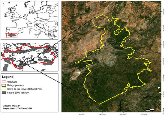
Figure 1.
Location of the study area. Enlarged figure shows the limits of the Sierra de las Nieves National and Natural Park. A map showing the Natura 2000 network in Andalusia (left bottom inset, grey area).
Approximately 4000 wildfire events were recorded in the province of Málaga during the 1988–2020 period, 65% of which burned areas of less than 1 ha. Almost all of these incidents were extinguished by fire-fighting forces.
2.2. Methodological Framework
This research was developed using a methodological framework divided into three steps to characterized each of the three fuel attributes assessed (Figure 2): biomass load, structural complexity, and live fuel moisture.
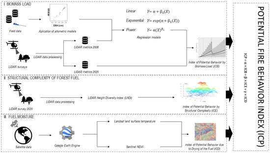
Figure 2.
Flowchart used to develop Wildfire Potential Behaviour Indices in complex Mediterranean forests.
2.3. Field Data
The field data used in this study were a local forest management inventory. Data from 450 plots (6.4% of the total study area) located on the forest perimeter “Sierra del Pinar”, which is completely within the limits of the study area (Supplementary Materials Figure S1), were used in this study. Circular plots were established at the intersections of a 200 × 200 m UTM grid for Pinus spp. forests and 167 × 167 m for Abies pinsapo forests with radii of 13 m. The diameter at breast height (dbh, 1.30 cm height) and total height (Ht) were measured for all trees of dbh ≥ 7.5 cm (Table 1). The shrub layer was estimated as area covered (%). The measurements were conducted in 2005.

Table 1.
Silvicultural variables of forest types in Sierra de las Nieves National Park (Málaga, southern Spain).
2.4. Forest Fuel Models
A map of fuel models was created by following Rothermel [14], based on the reclassification of previous land use cartography [32]. This cartograph was generated by means of photointerpretation of vegetation at 1:25,000 scale [32] (Figure 1, Supplementary Materials Table S1). Once forest fuel models were assigned to each vegetation polygon, additional information concerning vegetation cover, dominant and secondary tree species, shrub and herbaceous covers of a detail of 5–10% was added using REDIAM-SIOSE (2016, [32]). Information regarding the species composition of the shrub layer was obtained from the Spanish National Forest Map (1:50,000, [33]). Species with percentages of forest cover lower than 25% were eliminated. Finally, six forest types were considered (Supplementary Materials Table S2). Vegetation with forest cover lower than 10% was considered “not forests”. The forest fuel model map was developed using ArcGIS Pro 3.0 software and integrated into an ESRI format file geodatabase [34].
2.5. Remote Sensing Data
2.5.1. Airborne Laser Scanning Data
Airborne Laser Scanning (ALS) data were provided by Andalusian Environmental Information Network (REDIAM) and Spanish National Aerial Photography Programme (PNOA, [35]). The study area was surveyed in 2008 and 2020. ALS2008 data had an average point density of 2 pulses m−2, and ALS2020 had an average point density of 1.5 pulses m−2. The reference system employed was the European Terrestrial Reference System 89 (ETRS89) and UTM coordinate system. We assumed accurate georeferencing of 2008 and 2020 datasets during postprocessing and carried out no further co-registration. ALS2008 was divided into square tiles of 1 × 1 km (data are publicly available in the .las format at: https://portalrediam.cica.es/descargas/, accessed on 15 January 2020). ALS2020 data are provided in the .laz format, and each file comprises a square tile of 2 × 2 km (data are publicly available at: https://centrodedescargas.cnig.es/CentroDescargas/, accessed on 15 May 2023).
2.5.2. ALS Data Processing
ALS data were processed using a combination of FUSION LDV 3.50 [36] and LAStools v180520 [37] software. Raw ALS point clouds were converted into several intermediate products: DEM (Digital Elevation Model), normalised point clouds, and CHM (Canopy Height Model). This was done by first cleaning the noise from the point clouds. ALS points were classified as ground and non-ground (vegetation) returns using a morphological filter. Calculation of vegetation height was performed by employing the lasheight tool. The CloudMetrics tool was used to derive a suite of ALS canopy metrics. A complete description of ALS-derived canopy height metrics can be found in Mcgaughey [36].
2.5.3. Multispectral Images
Data preparation and image processing were performed with the Google Earth Engine (GEE, https://earthengine.google.com/, accessed on 1 June 2023), while the Earth Engine Python API was used to interact with Earth Engine Servers, using the Python programming language.
Landsat 8 and Sentinel 2-A images were used to calculate changes in fuel moisture. Surface temperature was calculated from images obtained by the TIRS sensor (Thermal Infrared Sensor) of the Landsat 8 satellite (band 10-TIRS-1, 100 m, https://earthexplorer.usgs.gov/, accessed on 15 May 2023). Surface temperature value (ºK) was obtained after previous processing of radiance registered by TIRS band 10. Information obtained by the ASTER sensor (Advanced Spaceborne Thermal Emission and Reflection Radiometer) on board the TERRA satellite was used as auxiliary information for this process, specifically the Global Emissivity Dataset (GED) product. GED has a global emissivity coverage with a spatial resolution of 100 m. Images corresponding to the 2 TIER1 catalogue (a higher level of quality control) and a processing level of 2 were used, corresponding to the elimination of atmospheric effects, for which the reflectivity at ground level was obtained.
Normalised Difference Vegetation Index (NDVI) was calculated from Sentinel 2-A images (Multi Spectral Instrument, 10 m, ESA, https://sentinels.copernicus.eu/web/sentinel/home, accessed on 16 May 2023).
2.6. Forest Fuel Characteristics
2.6.1. Biomass
Biomass load was calculated for each fuel model based on field data and allometric equations, both for tree and shrub layers. Three types of allometric equations were used: (i) allometric equations for Spanish coniferous forest species (input variables Ht and dbh, [38,39]); (ii) allometric equations for Spanish coniferous and hardwood species (input variable dbh [40]); and (iii) allometric equations for shrub species [41,42] (Supplementary Materials Table S3). Total biomass per plot was obtained by adding the biomass of trees and shrub strata.
Regression models were fitted to calculate the total biomass of each forest type using field inventory (Section 2.3) and ALS2008 metrics (Supplementary Materials Table S2) [43]. Once regression models were generated, a biomass map was obtained using ALS2020 metrics at a spatial resolution of 10 m. The cloudmetrics, CSV2grid, and mergeaster modules of FUSION and the ArcGIS Pro Model Builder tool were used during this process [34,36]. The 3-year time interval between the acquisition of field data (2005) and ALS2008 was considered negligible owing to forest-stand homogeneity and the low annual height and diameter growth in the study area.
2.6.2. Structural Complexity
Structural complexity of forest fuels was assessed by calculating the LiDAR Height Diversity Index (LHDI) regarding vegetation distribution and vertical diversity. LHDI is an index derived from the diversity index proposed by Shannon [44] and adapted by Listopad et al. [30] for estimation of biodiversity in plant formations (Equation (1)):
where ph is the proportion of returns in the height interval h with respect to the total number of returns.
Following Domingo et al. [45], we used a cell size of 10 m and a height interval of 0.5 m. In order to apply the LHDI equation, it was necessary to calculate the value of the product ph × ln(ph) in each of the tiles of the ALS point cloud, where ph is the value of each of the pixels in each of the height intervals considered. This process was conducted using a Python script and the ArcPy library of ArcGIS Pro [34] and ALS2020 data.
2.6.3. Fuel Moisture
Ful moisture was calculated using the index proposed by Chuvieco et al. [46], according to which the moisture of living fuel is strongly correlated with surface temperature and Normalized Difference Vegetation Index. This index was used based on the capacity of live fuels to retain or lose moisture throughout the year by analysing an annual multitemporal series image for a period between 2017 and 2021 (Section 2.5.3). The seasonal relative moisture index of live fuel (IRH) is expressed by Equation (2):
where Ts is the surface temperature of the vegetation or bare soil and NDVI is the value of the Normalized Difference Vegetation Index. NDVI and temperature and moisture indices were automated using the Google Earth Engine, Landsat 8 OLI-TIRS, and Sentinel 2-A catalogues. IRH was obtained for spring, and later summer. Annual drying index (IDA) was subsequently calculated as the difference between both values, which resulted in a raster dataset for each year. Finally, the fuel desiccation index (IDM) for the annual IDA series was obtained. This methodology was proposed owing to the absence of field fuel moisture data.
2.7. Potential Fire Behaviour Index
As a final part of the methodology, potential fire behaviour indices related to fuel attributes were generated, along with a synthetic global index of potential fire behaviour at a 10 m pixel scale throughout the study area:
- Potential Biomass Index (ICB): Fire danger associated with biomass load.
- Potential Structural Complexity Index (ICE): Fire danger associated with vegetation structure.
- Potential Fuel Desiccation Index (ICD): Fire danger associated with fuel moisture.
Thresholds were defined for each index to establish a common categorisation considering the distribution of normalised variable values. The categories of potential behaviour established were: (i) very low, (ii) low, (iii) moderate, (iv) high, and (v) very high.
The ICB, ICE, and ICD values were normalised, and a Potential Fire Behaviour Index (ICP) was obtained. The Potential Behaviour Index (ICP) was calculated as the weighted sum of the three partial indices (ICB, ICE, and ICD) (Equation (3)):
where ICP is the Potential Fire Behaviour Index, α is the weighting factor of the Potential Behaviour Biomass Index (ICB), β is the weighting factor of the Potential Behaviour Structural Complexity Index (ICE), and γ is the weighting factor of the Potential Behaviour Fuel Desiccation Index (ICD). The values of α, β, and γ were estimated by considering the relative weight that each of forest fuel variables have in fire behaviour, and the following values were therefore assigned as: α = 0.5, β = 0.3, and γ = 0.2 based on INFOCA expert assessment. ICP was mapped on a five-category scale, generating a fuel model map with additional information about potential fire behaviour. The resulting map was simplified by assigning an average value of the indices in each tile to the entire tile. The thresholds were subsequently applied to obtain the thematic maps with the levels of potential behaviour according to each index.
ICP = α × ICB + β × ICE + γ × ICD
3. Results
3.1. Fuel Model Map
Figure 3 shows the map of Rothermel’s fuel models obtained from the SIOSE 2016 (Table 2). The dominant fuel model in the area was Model 4, corresponding mainly to areas with the presence of Juniperus spp., following by Model 8, corresponding mainly to Pinus halepensis stands in the NE sector. Models 1 and 5 had relatively large areas, which corresponded mainly to grasslands located in the NW sector (Model 1) and to non-wooded shrubs in the central sector of the study area (Model 5). The remaining models (11 to 13) were not represented.
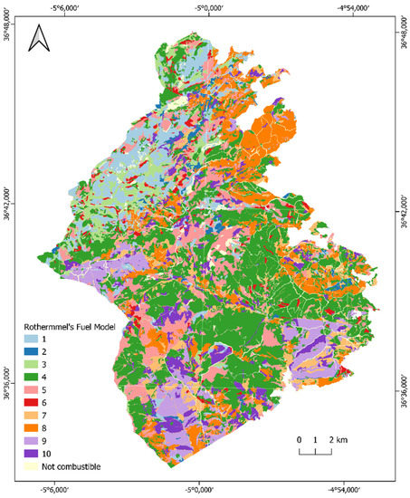
Figure 3.
Rothermmel’s fuel models of forest types in Sierra de las Nieves National Park (Málaga, southern Spain).
Table 2.
Rothermmel’s fuel models of forest types in Sierra de las Nieves National Park (Málaga, southern Spain).
3.2. Biomass Load of Forest Fuels
A biomass–ALS calibration model was used for the different forest types (Figure 4; see Supplementary Materials Table S2 for the selected metrics and model equations). The biomass models performed well for Abies pinsapo (R2 = 0.69), Juniperus spp. (R2 = 0.70), Pinus halepensis (R2 = 0.59), Pinus spp. mixed (R2 = 0.80), and Pinus spp.–Juniperus spp. (R2 = 0.59) forests.
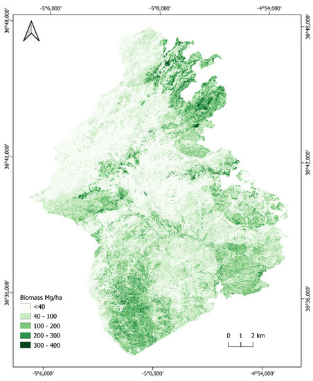
Figure 4.
Biomass of forest types in Sierra de las Nieves National Park (Málaga, southern Spain).
The highest values of biomass were obtained for Pinus halepensis forests (190.43 Mg ha−1), similar to other Pinus and evergreen Quercus forests (Table 2, Figure 4). However, the biomass of Abies pinsapo was, in relative terms, lower (53.77 Mg ha−1) than other wooded formations. Juniperus forests obtained intermediate values.
3.3. Structural Complexity
LHDI successfully differentiated among forest types (Figure 5; Table 3). The highest values of LHDI corresponded to Pinus spp.–evergreen (2.56), Q. suber (2.54), and Pinus mixed (2.49) forests, with the minimum being obtained for Juniperus (1.37) and shrubs (1.11).
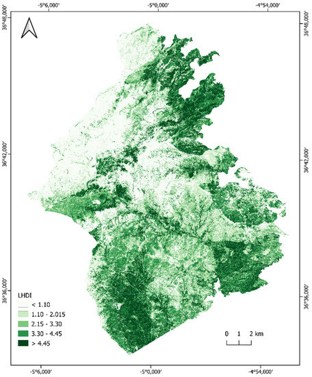
Figure 5.
LiDAR Height Diversity Index (LHDI) of forest types in Sierra de las Nieves National Park (Málaga, southern Spain).
Table 3.
Biomass, LiDAR Height Diversity Index (LHDI), and Fuel Desiccation Index (IDM) of forest types in Sierra de las Nieves National Park (Málaga, southern Spain). Mean ± standard deviation.
3.4. Fuel Desiccation Index (IDM)
The Fuel Desiccation Index (IDM), calculated as the temporal differences between a seasonal relative moisture index of live fuel (IRH) for spring and summer of each year, is showed in Figure 6. The minimum values of IDM were obtained for those areas dominated by shrubs (−396.71), with a maximum value for Pinus spp.–evergreen forests (−20.31) (Table 3).
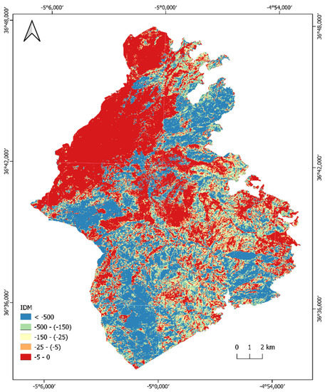
Figure 6.
Fuel Desiccation Index (IDM) of forest types in Sierra de las Nieves National Park (Málaga, southern Spain).
3.5. Potential Behaviour Indices
Biomass Index (ICB) values were high or very high for 11.86% of the area and low or very low for 77.07%. Structural Complexity Index (ICE) values were higher than ICB values and was high or very high for 37.23% of the area, and low or very low for 46.35%. Fuel Desiccation Index (ICD) was the opposite to ICB and ICE, with high or very high values for areas with a low biomass and a low structural complexity. The ICD value was high or very high for 45.93% of the area and low or very low for 44.50% (Table 4).
Table 4.
Surface (ha) and percentage (%) of Potential Behaviour Biomass Index (ICB), Potential Behaviour Structural Complexity Index (ICE), Potential Behaviour Fuel Desiccation Index (ICD), and Potential Fire Behaviour Index (ICP) of forest types in Sierra de las Nieves National Park (Málaga, southern Spain).
The ICP values were high or very high for 38.25% of the area, and low or very low for 45.96%. High or very high values were related to Pinus halepensis forests located in the north, Pinus pinaster forests located in the south, and mixed stands of Pinus pinaster and Quercus suber located in the east (Figure 7).
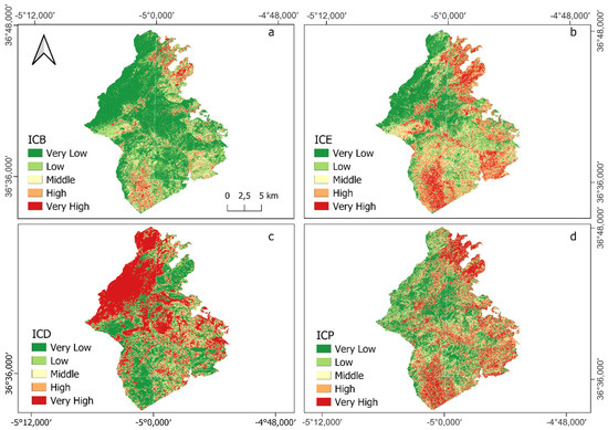
Figure 7.
(a) Potential Behaviour Biomass Index (ICB), (b) Potential Behaviour Structural Complexity Index (ICE), (c) Potential Behaviour Fuel Desiccation Index (ICD), and (d) Potential Fire Behaviour Index (ICP) of forest types in Sierra de las Nieves National Park (Málaga, southern Spain).
4. Discussion
Traditional maps of forest fuel models are useful tools in so far as they suppose a generalization of vegetation characteristics that allows their use in fire behaviour simulation tools [47]. However, numerous studies continue to provide highly descriptive cartographs that do not adequately represent the variation in forest fuels [48,49]. Although these maps are produced by means of photointerpretation at a detailed scale, a bias is introduced when assigning photo-interpreted covers to fuel models, especially in models under tree cover. Furthermore, these maps generally provide information regarding only fire behaviour in ground vegetation designed to simulate fire progression in conditions in which the forest canopy does not ignite. Some simulators, such as WildFire Analyst [50], already allow the integration of tree cover information, such as crown height, branches, or fuel load.
Remote sensing has been used for forest fuel mapping for more than two decades [6,17] at a lower cost and with highly accurate mapping products. However, cartography of forest fuel attributes that influence fire behaviour has many operational limitations [10]. These attributes are particularly important when attempting to characterize fuels in a quantitative and not only a qualitative manner, and for their use in fire behaviour models. It is, therefore, increasingly necessary to have metrics related to fire behaviour, and not only categorical forest fuel models using previous maps that were not necessarily developed for this purpose. This work proposes a methodology to improve fire fuels attributes maps by integrating field inventories, low density ALS, and satellite data in complex Mediterranean forests. Our results comprise maps of three key fire fuels attributes (biomass, vertical structure, and fuel moisture) that allow us to establish differences in potential fire behaviour. Thus, this cartograph can have a double use: as input in forest fire simulation modelling and for rapid detection of areas of special interest for wildfire prevention and extinction. The implications of these results depend on expectations about what forest fuel attribute maps communicate to decision makers and the nature of the decisions these maps are intended to inform.
4.1. Fuel Models and Biomass Load
The most frequently used fire fuel attributes are canopy height, structure (vertical and horizontal), fuel moisture, and fuel load (biomass) [10]. The mapping of fuel attributes, therefore, plays a larger role than simply determining fuel models [51,52]. Biomass is needed to estimated forests fuel loads. Fuel models serve as conventional approaches to biomass estimation, which, despite being a simpler approach, typically restrict spatial and temporal projections. Advances in LiDAR-ALS technology, which provides detailed information on vegetation structure, have made it possible to improve the estimation of fuel biomass attributes [52,53,54]. Integration of ALS and allometric models allows a better biomass estimation, which is essential to understand fuel load and its vertical and horizontal continuity. In the study area, the aboveground biomass of tree covers ranged from 190.43 Mg ha−1 (Pinus halepensis forests) to 53.77 Mg ha−1 (Abies pinsapo and Abies pinsapo-Quercus spp. forests). Those values are similar to other studies of Mediterranean forests [40,55,56]. ALS biomass models included metrics associated with height indicating different levels of LiDAR penetration [55,57]. Additional variables related to canopy cover and structure (standard deviation of the height distribution) were also included (Table S2). Empirical models derived from height data were used to estimate biomass load (Table 2). The selection of various height percentiles for various type of forests reflects the structural differences that exist between them, as evidenced by return distribution [58,59]. Our findings are consistent with previous research which found a strong correlation of biomass fuel load with ALS height metrics.
4.2. Structural Complexity of Forest Fuels
Vegetation structural complexity has a great influence on fire severity [45]. The presence of a continuous vertical layer of vegetation, formed as both a shrub layer and tree cover (low dead branches, species with ramifications close to the ground, etc.) facilitates fire transition from the surface to tree crown [29]. Depending on fire conditions, such as topography or wind intensity, fuel vertical continuity can lead to an energetic behaviour of the flame front, which prevents its extinction from land or air. A structural complexity analysis approach based on ALS data allows the inclusion of vertical and horizontal fuel structures, aspects that are very difficult to include when using approaches based on field data [58]. This approach provides a better understanding of fire behaviour based on LiDAR data analysis techniques with a high spatial resolution [59].
Vegetation structural complexity has been analysed in terms of diversity by Shannon [44], while Listopad et al. [30] transferred these equations to LiDAR data, assimilating vertical vegetation distribution to the LiDAR cloud. Previous studies have shown the ability of these LiDAR-derived indices to assess the structural characteristics of forests [28,60]. Here, we used the LiDAR Height Diversity Index (LHDI). This index expresses the level of vegetation homogeneity in the vertical distribution of returns. Comparisons of the results obtained in this study with similar data from other sites are limited because of the novelty of the method. While recognizing the limitations of comparisons, it is noteworthy that LHDI values obtained for complex Mediterranean forests were consistent with the expected vegetation structure of forest types. The highest values of LHDI were obtained for Quercus suber, mixed Pinus, and Pinus and broadleaved forests. However, differences between forest types were not significant, only between forest and non-forest types dominated by smaller species such as Juniperus. When applying LHDI to the Potential Behaviour Structural Complexity Index (ICE), high or very high values were obtained for 37.23% of the area. Once again, there was a correspondence between high and extremely high values with Pinus halepensis and Pinus pinaster forests located in the northern and southern areas, although Quercus suber forests also obtained high ICE values. Low and very low values covered 38.35% of the area, corresponding to low tree cover forests, which were, therefore, those with less structural complexity. The LiDAR Height Diversity Index contributed to the description of the vertical forest structure based on ALS in a practical way [57,61], facilitating its generalization to large surfaces, and with levels of information similar to much more complex systems.
4.3. Fuel Moisture
Fuel moisture, which is understood as the ratio between the total weight and the dry weight of the vegetation in live and dead fractions, is another fuel attribute that influences fire severity and behaviour [62]. The proportion of the front flame energy invested in evaporation of fuel moisture determines the remaining energy available for combustion of other volatiles and the solid vegetation fraction [59]. Fuel moisture is strongly correlated with climate, such as temperature, relative moisture, or prevailing winds. However, there are intrinsic vegetation factors that determine the ability of the vegetation to retain or lose moisture [63], such as species composition (morphological, physiological, etc.), and factors related to vegetation structure (fraction of area covered, age, etc.).
A fuel desiccation index was generated partially based on the workflow of Chuvieco et al. [46] and Romero Ramirez et al. [12]. The objective of the fuel desiccation index (IDM) proposed in this study is to assess the fuel based on the relative differences between forest types in terms of the ability to retain or lose moisture. IDM was sensitive to moisture content of dead fuel, as could be observed from the results obtained for annual seasonal moisture indices in areas dominated by grass. Fuel Desiccation Index (ICD) values were high or very high in 45.93% of grass and scrub areas. This would appear to indicate a correlation between ICD and the moisture content of dead fuels. On the contrary, 44.50% of the area obtained low or very low ICD values, which were related to areas with higher biomass and structural complexity values. These factors could contribute to changes in fuel moisture, through radiation levels or exposure to drying winds. Estimating fuel moisture is significantly complicated by vegetation spatial heterogeneity [20,64], which may be simplified by aggregating species in dominant forest types. Finally, heterogeneous vegetation type composition altered the temporal moisture response of vegetation. Using a temporal image series based on the Google Earth Engine (GEE) platform simplified the operational image data analysis [65].
4.4. Potential Forest Fire Behaviour Index
The understanding of fuel attributes and their relationship with fire behaviour is needed [66]. In this study, a Potential Fire Behaviour Index (ICP) was proposed. A relative weight of three fuel attributes (biomass, structural complexity, and fuel moisture) was considered to assess potential fire behaviour. Biomass was considered to be the principal fuel attribute (0.5), since it is the major factor in regard to determining energetic fire behaviour. High or very high ICP values were obtained in 37.25% of the total area, when compared to 44.96% for which the values were low or very low. The areas with the highest ICP value corresponded to Pinus halepensis and Pinus pinaster forests, although high values were also found for stands of Abies pinsapo forests. Our findings suggest that ICP can provide reliable information about which landscape locations are most prone to fire due to the vegetation strongly regulating fires in the Mediterranean area [67].
Based on well-established fuel model strategies, maps of fire fuel attributes provide a means of comprehending differences in potential fire behaviour either through direct interpretation of cartography or by incorporation into fire simulators. Important management implications arise from the ability to differentiate stands based on their potential response to fire initiation and spread. To map fuel hazards and prioritize locations where fuel reduction or removal could be used to reduce risk, it is necessary to identify stands with particular fuel attributes [64]. In the same direction, stands with complex fuel structures with hazardous fuels can be assessed for large landscapes using key fuel attributes and low-cost data. The use of simple landscape fire fuel attributes maps has been sparse, possibly as a result of a prevalent fire risk modelling paradigm that mandates probabilistic assessments of fire likelihood. However, our map-based approaches using a numerical rating of potential for fire transmission based on fuel biomass, structure, and moisture configuration simplified the computationally complicated and data-intensive methods that are used to characterize potential fire spread across landscapes. Complex probabilistic modelling efforts may yield little insight into which locations can be expected to burn over the next few years either due to a low fire incidence or the random nature of many of them in high-risk conditions in which the likelihood of burning is low, such as boreal forests [68,69]. These highlight the fact that probabilities are not appropriate for describing the risk of rare events with potential catastrophic effects and recommend qualitative methods or possibilistic measures in these situations. Therefore, the integration of field and remote sensing data allows the development of maps for fire management and firefighting based on expert knowledge and experience and fire behaviour modelling, through a rapid and updateable description of fuel attributes, such as fuel load, canopy height, and vegetation flammability.
4.5. Limitations
Our study characterized forest fuel attributes in a region particularly suited to unravelling the factors that modulate fire behaviour, due to the diversity of landscapes and vegetation formations. Additionally, we leveraged a robust collection of remote sensing data to quantify the components of forest fuel attributes. However, it is important to recognize the inherent limitations of our study. First, this study lacks field data to validate our results, due to the non-occurrence of forest fires in the study area. Nevertheless, there are good conceptual and empirical arguments that support our conclusions about the factors controlling the behaviour of forest fires and their quantification. Second, our forest fire behaviour index ignores information about topographic conditions, such as slope or aspect, which are known to influence fire behaviour. For a given fuel type, slope can be expected to accelerate combustion and fire spread rates in comparison with flat terrain [70]. We suspect that locations exposed to hazardous fuel will burn, irrespective of the contribution of slope or other topographic variables towards combustion rates. and therefore, these variables have a minimal influence on the fire behaviour index [70]. Third and perhaps most fundamentally important, we assigned the three different weights described in the estimation of the ICP based on the experience of INFOCA’s expert firefighting personnel. This problem is partly related to the previously above-mentioned scarcity of field data. However, we believe that the weights assigned for each of the three forest fuel attributes produced results consistent with those obtained by other authors. For example, Age and Skinner [71] showed that above-ground biomass (fuel load) is the most important contributor to fire behaviour. Furthermore, Rothermel [14] and Pimont et al. [72] found that in addition to fuel load, the spatial continuity (structural complexity) and moisture of these fuels strongly influences fire behaviour.
4.6. Applications
The resulting maps can offer cartographs to help wildland firefighters which do not always (or almost never) have the capacity to generate “real time” simulations in prevention and extinction actions. In determining whether or not to invest in a computationally and time-intensive modelling exercise, prospective users of these maps should consider whether or not a fire behaviour map with just three fuel attributes (load, structural complexity, and moisture) is useful for informing their decisions [73]. Nevertheless, these maps should be used with caution with consideration of their shortcomings and apparent limitations.
5. Conclusions
In this study, a new forest fire behaviour index based on fuel data using various attributes including fuel load, moisture, and structural complexity was proposed. Remote sensing was applied to improve fuel attribute characterisation and cartography, highlighting the utility of integrating multispectral and ALS data to estimate those attributes that are more closely related to the spatial organisation of vegetation (for example, canopy height, biomass, structural complexity, and moisture). The application of this methodology to the mapping of forest fuel models makes it possible to obtain attributes at an adequate spatial resolution by combining sensors that have already proved to be useful for the estimation of forest fuels during the last decade (COPERNICUS Program) with field data and low-density ALS data. The use of ALS data for forest fuel catheterization has become widespread in the last decade due to cost reduction and improvement of data analysis. Since the indices proposed are based on freely available remote sensing data, this method is transferable to other territories and different spatial scales. Despite the numerous limitations of these fuel data, pre-existing, coarse-scale fuel type data are insufficient for accurately assessing the spatial variation in fire management. Even though most of the variables that are commonly used to evaluate potential fire behaviour and fire likelihood at the landscape scale—such as topography, weather, wind speed and direction, season, and fire regime characteristics typically derived from historical data—were omitted from our fuel fire exposure metric, it still offers practical applications for guiding fire management decisions like proactive vegetation management and evacuation planning. The exposure metrics will need further evaluation before it can be used in other ecosystems that differ from our study area, despite the promising findings of our study.
Supplementary Materials
The following are available online at https://www.mdpi.com/article/10.3390/rs15082023/s1, Table S1. Forest types and fuel models present in Sierra de las Nieves National Park (Málaga, southern Spain); Table S2. ALS-derived metrics for biomass models of forest types in Sierra de las Nieves National Park (Málaga, Southern Spain); Table S3. Allometric equations for tree species used in the calculation of the aerial biomass load of the forest inventory plots. Diameter at breast height (d, 1.30 cm height) and total height (h).
Author Contributions
Conceptualisation, R.C.C. and R.M.N.-C.; methodology, R.C.C., R.M.N.-C. and M.Á.V.M.; formal analysis, R.C.C., M.Á.V.M., A.J.A.S. and F.R.G.; investigation, R.C.C. and R.M.N.-C.; resources, R.C.C.; data cleaning, R.C.C., M.Á.V.M. and F.R.G.; writing—original draft preparation, R.M.N.-C., R.C.C. and A.J.A.S.; writing—review and editing, all authors; supervision, R.M.N.-C.; project administration, R.C.C.; acquisition of funding, R.C.C. All authors have read and agreed to the published version of the manuscript.
Funding
This research was funded by Ministerio de Ciencia e Innovación (Spain) through the projects SILVADAPT.NET (RED2018-102719-T), EVIDENCE (Ref: 2822/2021) and REMEDIO (PID2021-128463OB-I00).
Institutional Review Board Statement
Not applicable.
Informed Consent Statement
Not applicable.
Data Availability Statement
The data presented in this study are available on request from the corresponding author. The data are not publicly available owing to institutional restrictions.
Acknowledgments
We would like to acknowledge the support provided by SILVADAPT.NET (RED2018-102719-T), EVIDENCE (Ref: 2822/2021), and REMEDIO (PID2021-128463OB-I00). We would also like to acknowledge the financial and institutional support of the University of Cordoba-Campus de Excelencia CEIA3. The authors acknowledge and thank the Mediterranean Forest Global Change Observatory for its support through the “Scientific Infrastructures for Global Change Monitoring and Adaptation in Andalusia (INDALO)—LIFEWATCH-2019-04-AMA-01” project, which was co-financed with FEDER funds corresponding to the Pluriregional Operational Programme of Spain 2014–2020. We are very grateful to the “Consejería de Medioambiente y Ordenación del Territorio” (Junta de Andalucía) and the “RED SEDA NETWORK” (Junta de Andalucía), for providing field work and data support.
Conflicts of Interest
The authors declare no conflict of interest.
References
- Lasslop, G.; Coppola, A.I.; Voulgarakis, A.; Yue, C.; Veraverbeke, S. Influence of Fire on the Carbon Cycle and Climate. Curr. Clim. Change Rep. 2019, 5, 112–123. [Google Scholar] [CrossRef]
- Mohajane, M.; Costache, R.; Karimi, F.; Bao Pham, Q.; Essahlaoui, A.; Nguyen, H.; Laneve, G.; Oudija, F. Application of remote sensing and machine learning algorithms for forest fire mapping in a Mediterranean area. Ecol. Indic. 2021, 129, 107869. [Google Scholar] [CrossRef]
- Ghorbanzadeh, O.; Blaschke, T.; Gholamnia, K.; Aryal, J. Forest Fire Susceptibility and Risk Mapping Using Social/Infrastructural Vulnerability and Environmental Variables. Fire 2019, 2, 50. [Google Scholar] [CrossRef]
- Han, S.; Han, Y.; Jin, Y.; Zhou, W. The method for calculating forest fire behaviour index. Fire Saf. Sci. 1992, 1, 77–82. [Google Scholar]
- Atchley, A.L.; Linn, R.; Jonko, A.; Hoffman, C.; Hyman, J.D.; Pimont, F.; Sieg, C.; Middleton, R.S. Effects of fuel spatial distribution on wildland fire behaviour. Int. J. Wildland Fire 2021, 30, 179–189. [Google Scholar] [CrossRef]
- Gale, M.G.; Cary, G.J.; van Dijk, A.I.J.M.; Yebra, M. Forest fire fuel through the lens of remote sensing: Review of approaches, challenges and future directions in the remote sensing of biotic determinants of fire behaviour. Remote. Sens. Environ. 2021, 255, 112282. [Google Scholar] [CrossRef]
- Gonzalez-Olabarria, J.R.; Reynolds, K.M.; Larrañaga, A.; Garcia-Gonzalo, J.; Busquets, E.; Pique, M. Strategic and tactical planning to improve suppression efforts against large forest fires in the Catalonia region of Spain. For. Ecol. Manag. 2018, 432, 612–622. [Google Scholar] [CrossRef]
- Hesseln, H. Wildland Fire Prevention: A Review. Curr. For. Rep. 2018, 4, 178–190. [Google Scholar] [CrossRef]
- Hély, C.; Flannigan, M.; Bergeron, Y.; McRae, D. Role of vegetation and weather on fire behaviour in the Canadian mixedwood boreal forest using two fire behaviour prediction systems. Can. J. For. Res. 2001, 31, 430–441. [Google Scholar] [CrossRef]
- Arroyo, L.A.; Pascual, C.; Manzanera, J.A. Fire models and methods to map fuel types: The role of remote sensing. For. Ecol. Manag. 2008, 256, 1239–1252. [Google Scholar] [CrossRef]
- Preisler, H.K.; Weise, D.R. Forest Fire Models. Encyclopedia of Environmetrics; John Wiley & Sons, Ltd.: Hoboken, NJ, USA, 2001. [Google Scholar]
- Romero Ramirez, F.J.; Navarro-Cerrillo, R.M.; Varo-Martínez, M.Á.; Quero, J.L.; Doerr, S.; Hernández-Clemente, R. Determination of forest fuels characteristics in mortality-affected Pinus forests using integrated hyperspectral and ALS data. Int. J. Appl. Earth Obs. Geoinf. 2018, 68, 157–167. [Google Scholar] [CrossRef]
- Sullivan, A.L. Inside the Inferno: Fundamental Processes of Wildland Fire Behaviour: Part 2: Heat Transfer and Interactions. Curr. For. Rep. 2017, 3, 150–171. [Google Scholar] [CrossRef]
- Rothermel, R.C. A Mathematical Model for Predicting Fire Spread in Wildland Fuels; Research Paper INT-115; U.S. Department of Agriculture, Intermountain Forest and Range Experiment Station: Ogden, UT, USA, 1972; Volume 115, 40p.
- Pastor, E.; Zárate, L.; Planas, E.; Arnaldos, J. Mathematical models and calculation systems for the study of wildland fire behaviour. PECS 2003, 29, 139–153. [Google Scholar] [CrossRef]
- Zylstra, P.; Bradstock, R.A.; Bedward, M.; Penman, T.D.; Doherty, M.D.; Weber, R.O.; Gill, A.M.; Cary, G.J. Biophysical mechanistic modelling quantifies the effects of plant traits on fire severity: Species, not surface fuel loads, determine flame dimensions in eucalypt forests. PLoS ONE 2016, 11, e0160715. [Google Scholar] [CrossRef]
- Chuvieco, E.; Aguado, I.; Salas, J.; García, M.; Yebra, M.; Oliva, P. Satellite Remote Sensing Contributions to Wildland Fire Science and Management. Curr. For. Rep. 2020, 6, 81–96. [Google Scholar] [CrossRef]
- Skowronski, N.S.; Gallagher, M.R.; Warner, T.A. Decomposing the interactions between fire severity and canopy fuel structure using multi-temporal, active, and passive remote sensing approaches. Fire 2020, 3, 7. [Google Scholar] [CrossRef]
- Campbell, J.B.; Wynne, R.H. Introduction to Remote Sensing; Guilford Press: New York, NY, USA, 2011. [Google Scholar]
- Yebra, M.; Dennison, P.E.; Chuvieco, E.; Riaño, D.; Zylstra, P.; Hunt, E.R., Jr.; Danson, F.M.; Qi, Y.; Jurdao, S. A global review of remote sensing of live fuel moisture content for fire danger assessment: Moving towards operational products. Remote Sens. Environ. 2013, 136, 455–468. [Google Scholar] [CrossRef]
- Chuvieco, E.; Riaño, D.; Van Wagtendok, J.; Morsdof, F. Fuel Loads and Fuel Type Mapping. In Wildland Fire Danger Estimation and Mapping: The Role of Remote Sensing Data; World Scientific: London, UK, 2003; pp. 119–142. [Google Scholar]
- Wang, P.; Wang, J.; Chen, Y.; Ni, G. Rapid processing of remote sensing images based on cloud computing. Future Gener. Comput. Syst. 2013, 29, 1963–1968. [Google Scholar] [CrossRef]
- Saatchi, S.; Halligan, K.; Despain, D.G.; Crabtree, R.L. Estimation of forest fuel load from radar remote sensing. IEEE Trans. Geosci. Remote Sens. 2007, 45, 1726–1740. [Google Scholar] [CrossRef]
- Andersen, H.E.; McGaughey, R.J.; Reutebuch, S.E. Estimating Forest canopy fuel parameters using LIDAR data. Remote Sens. Environ. 2005, 94, 441–449. [Google Scholar] [CrossRef]
- İnan, M.; Bilici, E.; Akay, A.E.; İnan, M.; Bilici, E.; Akay, A.E. Using Airborne LIDAR Data for Assessment of Forest Fire Fuel Load Potential. ISPAN 2017, 4W4, 255–258. [Google Scholar] [CrossRef]
- Huesca, M.; Riaño, D.; Ustin, S.L. Spectral mapping methods applied to LiDAR data: Application to fuel type mapping. Int. J. Appl. Earth Obs. Geoinf. 2018, 74, 159–168. [Google Scholar] [CrossRef]
- Marino, E.; Ranz, P.; Tomé, J.L.; Noriega, M.Á.; Esteban, J.; Madrigal, J. Generation of high-resolution fuel model maps from discrete airborne laser scanner and Landsat-8 OLI: A low-cost and highly updated methodology for large areas. Remote Sens. Environ. 2016, 187, 267–280. [Google Scholar] [CrossRef]
- Gelabert, P.J.; Montealegre, A.L.; Lamelas, M.T.; Domingo, D. Forest structural diversity characterization in Mediterranean landscapes affected by fires using Airborne Laser Scanning data. GISci. Remote Sens. 2020, 57, 497–509. [Google Scholar] [CrossRef]
- Moinuddin, K.A.M.; Sutherland, D. Modelling of tree fires and fires transitioning from the forest floor to the canopy with a physics-based model. Math. Comput. Simul. 2020, 175, 81–95. [Google Scholar] [CrossRef]
- Listopad, C.M.C.S.; Masters, R.E.; Drake, J.; Weishampel, J.; Branquinho, C. Structural diversity indices based on airborne LiDAR as ecological indicators for managing highly dynamic landscapes. Ecol. Indic. 2015, 57, 268–279. [Google Scholar] [CrossRef]
- Cabezudo, B.; Solanas, F.C.; Pérez Latorre, A.V. Vascular flora of the Sierra de las Nieves National Park and its surroundings (Andalusia, Spain). Phytotaxa 2022, 534, 1–111. [Google Scholar] [CrossRef]
- Red de Información Ambiental de Andalucía. Base Cartográfica SIOSE Andalucía 2016. Ocupación del Suelo; Red de Información Ambiental de Andalucía: Sevilla, Spain; Sistema de Información sobre el Patrimonio Natural de Andalucía, SIPNA Publicación: Sevilla, Spain, 2020. [Google Scholar]
- MITECO. Spanish National Forest Inventory; MITECO: Madrid, Spain, 2022.
- ESRI. 2022. Available online: https://www.esri.com/es-es/home (accessed on 21 January 2020).
- Centro Nacional de Información Geográfica. Segunda Cobertura LiDAR Nacional; CNIG: Madrid, Spain, 2022. [Google Scholar]
- McGaughey, R.J. FUSION/LDV: Software for LIDAR Data Analysis and Visualization; USDA Forest Service, PNW: Washington, DC, USA, 2007; pp. 28–30.
- Isenburg, M. LAStools; Rapidlasso GmbH: Gilching, Germany, 2017. [Google Scholar]
- Ruiz-Peinado, R.; del Rio, M.; Montero, G. New models for estimating the carbon sink capacity of Spanish softwood species. Forest Syst. 2011, 20, 176–188. [Google Scholar] [CrossRef]
- Ruiz-Peinado, R.; Montero, G.; del Rio, M. Biomass models to estimate carbon stocks for hardwood tree species. Forest Systems 2012, 21, 42–52. [Google Scholar] [CrossRef]
- Montero, G.; Ruiz-Peinado, R.; Muñoz, M. Producción de Biomasa y Fijación de CO2 por los Bosques Españoles; Monografías13; INIA: Madrid, Spain, 2005. [Google Scholar]
- Navarro Cerrillo, R.M.; Blanco Oyonarte, P. Estimation of above-ground biomass in shrubland ecosystems of southern Spain. Investig. Agraria Sist. Y Recur. For. 2006, 15, 197–207. [Google Scholar] [CrossRef]
- Pasalodos-Tato, M.; Ruiz-Peinado, R.; del Río, M.; Montero, G. Shrub biomass accumulation and growth rate models to quantify carbon stocks and fluxes for the Mediterranean region. Eur. J. For. Res. 2015, 134, 537–553. [Google Scholar] [CrossRef]
- Ene, L.T.; Næsset, E.; Gobakken, T.; Gregoire, T.G.; Ståhl, G.; Nelson, R. Assessing the accuracy of regional LiDAR-based biomass estimation using a simulation approach. Remote Sens. Environ. 2012, 123, 579–592. [Google Scholar] [CrossRef]
- Shannon, C.E. A mathematical theory of communication. Bell Syst. Tech. J. 1948, 27, 379–423. [Google Scholar] [CrossRef]
- Domingo, D.; Lamelas, M.T.; García, M.B. Characterization of vegetation structural changes using multi-temporal LiDAR and its relationship with severity in Calcena wildfire. Ecosistemas 2021, 30, 1–10. [Google Scholar] [CrossRef]
- Chuvieco, E.; Cocero, D.; Riaño, D.; Martin, P.; Martínez-Vega, J.; de La Riva, J.; Pérez, F. Combining NDVI and surface temperature for the estimation of live fuel moisture content in forest fire danger rating. Remote Sens. Environ. 2004, 92, 322–331. [Google Scholar] [CrossRef]
- Scott, J.H.; Burgan, R.E. Standard Fire Behaviour Fuel Models: A Comprehensive Set for Use with Rothermel’s Surface Fire Spread Model; Gen. Tech. Rep. RMRS-GTR-153; U.S. Department of Agriculture, Forest Service, Rocky Mountain Research Station: Fort Collins, CO, USA, 2005; Volume 153, 72p.
- Novo, A.; Fariñas-Álvarez, N.; Martínez-Sánchez, J.; González-Jorge, H.; Fernández-Alonso, J.M.; Lorenzo, H. Mapping Forest fire risk—A case study in Galicia (Spain). Remote Sens. 2020, 12, 3705. [Google Scholar] [CrossRef]
- Sandberg, D.V.; Ottmar, R.D.; Cushon, G.H. Characterizing fuels in the 21st Century. Int. J. Wildland Fire 2001, 10, 381–387. [Google Scholar] [CrossRef]
- Tecnosylva S.L. WildFire Analyst (2.9); Tecnosylva S.L.: León, Spain, 2014. [Google Scholar]
- Duff, T.; Keane, R.; Penman, T.; Tolhurst, K. Revisiting Wildland Fire Fuel Quantification Methods: The Challenge of Understanding a Dynamic, Biotic Entity. Forests 2017, 8, 351. [Google Scholar] [CrossRef]
- Cheney, N.P.; Gould, J.S.; McCaw, W.L.; Anderson, W.R. Predicting fire behaviour in dry eucalypt forest in southern Australia. For. Ecol. Manag. 2012, 280, 120–131. [Google Scholar] [CrossRef]
- Luo, S.; Wang, C.; Xi, X.; Nie, S.; Fan, X.; Chen, H.; Ma, D.; Liu, J.; Zou, J.; Lin, Y.; et al. Estimating Forest aboveground biomass using small-footprint full-waveform airborne LiDAR data. Int. J. Appl. Earth Obs. Geoinf. 2019, 83, 101922. [Google Scholar] [CrossRef]
- Nie, S.; Wang, C.; Zeng, H.; Xi, X.; Li, G. Above-ground biomass estimation using airborne discrete-return and full-waveform LiDAR data in a coniferous forest. Ecol. Ind. 2017, 78, 221–228. [Google Scholar] [CrossRef]
- García, M.; Riaño, D.; Chuvieco, E.; Danson, F.M. Estimating biomass carbon stocks for a Mediterranean forest in central Spain using LiDAR height and intensity data. Remote Sens. Environ. 2010, 114, 816–830. [Google Scholar] [CrossRef]
- Guerra-Hernández, J.; Narine, L.L.; Pascual, A.; Gonzalez-Ferreiro, E.; Botequim, B.; Malambo, L.; Godinho, S. Aboveground biomass mapping by integrating ICESat-2, SENTINEL-1, SENTINEL-2, ALOS2/PALSAR2, and topographic information in Mediterranean forests. Remote Sens. 2022, 59, 1509–1533. [Google Scholar] [CrossRef]
- Domingo, D.; Alonso, R.; Lamelas, M.T.; Montealegre, A.L.; Rodríguez, F.; de la Riva, J. Temporal transferability of pine forest attributes modeling using low-density airborne laser scanning data. Remote. Sens. 2019, 11, 261. [Google Scholar] [CrossRef]
- Mauro, F.; Hudak, A.T.; Fekety, P.A.; Frank, B.; Temesgen, H.; Bell, D.M.; McCarley, T.R. Regional modelling of forest fuels and structural attributes using airborne laser scanning data in Oregon. Remote Sens. 2021, 13, 261. [Google Scholar] [CrossRef]
- Marino, E.; Montes, F.; Tomé, J.L.; Navarro, J.A.; Hernando, C. Vertical Forest structure analysis for wildfire prevention: Comparing airborne laser scanning data and stereoscopic hemispherical images. Int. J. Appl. Earth Obs. Geoinf. 2018, 73, 438–449. [Google Scholar] [CrossRef]
- Domingo, D.; de la Riva, J.; Lamelas, M.T.; García-Martín, A.; Ibarra, P.; Echeverría, M.; Hoffrén, R. Fuel type classification using airborne laser scanning and Sentinel 2 data in Mediterranean forest affected by wildfires. Remote Sens. 2020, 12, 3660. [Google Scholar] [CrossRef]
- Wulder, M.A.; White, J.C.; Nelson, R.F.; Næsset, E.; Ørka, H.O.; Coops, N.C.; Hilker, T.; Bater, C.W.; Gobakken, T. Lidar sampling for large-area forest characterization: A review. Remote Sens. Environ. 2012, 121, 196–209. [Google Scholar] [CrossRef]
- Kucuk, O.; Saglam, B.; Bilgili, E. Canopy fuel characteristics and fuel load in young black pine trees. Biotechnol. Biotechnol. Equip. 2007, 21, 235–240. [Google Scholar] [CrossRef]
- Hudak, A.T.; Bright, B.C.; Pokswinski, S.M.; Loudermilk, E.L.; O’Brien, J.J.; Hornsby, B.S.; Klauberg, C.; Silva, C.A. Mapping Forest Structure and Composition from Low-Density LiDAR for Informed Forest, Fuel, and Fire Management at Eglin Air Force Base, Florida, USA. Can. J. Remote Sens. 2016, 42, 411–427. [Google Scholar] [CrossRef]
- Qi, Y.; Dennison, P.E.; Spencer, J.; Riaño, D. Monitoring live fuel moisture using soil moisture and remote sensing proxies. Fire Ecol. 2012, 8, 71–87. [Google Scholar] [CrossRef]
- Quintero, N.; Viedma, O.; Urbieta, I.R.; Moreno, J.M. Assessing landscape fire hazard by multitemporal automatic classification of landsat time series using the Google Earth Engine in West-Central Spain. Forests 2019, 10, 518. [Google Scholar] [CrossRef]
- Jolly, W.M. Sensitivity of a fire behaviour model to changes in live fuel moisture. In Proceedings of the Sixth Symposium on Fire and Forest Meteorology, Canmore, AB, Canada, 24–27 October 2005. [Google Scholar]
- Fares, S.; Bajocco, S.; Salvati, L.; Camarretta, N.; Dupuy, J.L.; Xanthopoulos, G.; Corona, P. Characterizing potential wildland fire fuel in live vegetation in the Mediterranean region. Ann. For. Sci. 2017, 74, 1. [Google Scholar] [CrossRef]
- Beverly, J.L.; McLoughlin, N.; Chapman, E. A simple metric of landscape fire exposure. Landsc. Ecol. 2021, 36, 785–801. [Google Scholar] [CrossRef]
- Beverly, J.L.; McLoughlin, N. Burn probability simulation and subsequent wildland fire activity in Alberta, Canada—Implications for risk assessment and strategic planning. For. Ecol. Manag. 2019, 451, 117490. [Google Scholar] [CrossRef]
- Van Wagtendonk, J.W. Fire as a physical process. In Fire in California’s Ecosystems; Sugihara, N.G., van Wagtendonk, J.W., Fites-Kaufman, J., Shaffer, K.E., Thode, A.E., Eds.; University of California Press: Berkeley, CA, USA, 2006; pp. 38–57. [Google Scholar]
- Agee, J.K.; Skinner, C. Basic principles of forest fuel reduction treatments. Forest Ecol. Manag. 2005, 211, 83–96. [Google Scholar] [CrossRef]
- Pimont, F.; Dupuy, J.L.; Linn, R.R.; Dupont, S. Impacts of tree canopy structure on wind flows and fire propagation simulated with FIRETEC. Ann. For. Sci. 2011, 68, 523–530. [Google Scholar] [CrossRef]
- Sakellariou, S.; Sfougaris, A.; Christopoulou, O.; Tampekis, S. Integrated wildfire risk assessment of natural and anthropogenic ecosystems based on simulation modeling and remotely sensed data fusion. IJDRR 2022, 78, 103129. [Google Scholar] [CrossRef]


Disclaimer/Publisher’s Note: The statements, opinions and data contained in all publications are solely those of the individual author(s) and contributor(s) and not of MDPI and/or the editor(s). MDPI and/or the editor(s) disclaim responsibility for any injury to people or property resulting from any ideas, methods, instructions or products referred to in the content. |
© 2023 by the authors. Licensee MDPI, Basel, Switzerland. This article is an open access article distributed under the terms and conditions of the Creative Commons Attribution (CC BY) license (https://creativecommons.org/licenses/by/4.0/).