Spatial–Temporal Fusion of 10-Min Aerosol Optical Depth Products with the GEO–LEO Satellite Joint Observations

Abstract

Geosynchronous equatorial orbit (GEO) satellite-derived AOD possesses huge advantages for monitoring atmospheric aerosol with high frequency; however, the data missing existing in the satellite-derived AOD products dramatically limits this expected advantage due to cloud obscuration and aerosol retrieval algorithm. In recent years, numerous AOD fusion algorithms have been proposed, while these algorithms are mostly developed to blend daily AOD products derived from low Earth orbit (LEO) satellites and generally neglect discrepancies from different categories of products. Therefore, a spatiotemporal fusion framework based on the Bayesian maximum entropy theorem, blending GEO with LEO satellite observations and incorporating data discrepancies (GL-BME), is developed to complementarily recover the Advanced Himawari-8 Imager (AHI) AOD products over East Asia. The results show that GL-BME significantly improves the average spatial completeness of AOD from 20.3% to 67.6% with ensured reliability, and the accuracy of merged AODs nearly maintains that of original AHI AODs. Moreover, a comparison of the monthly aerosol spatial distribution between the merged and original AHI AODs is conducted to evaluate the performance and significance of GL-BME, which indicates that GL-BME could further restore the real atmospheric aerosol situation to a certain extent on the basis of dramatic spatial coverage improvement.

1. Introduction

Atmospheric aerosols are multiphase systems consisting of solid and liquid particles and gaseous carriers suspended in the atmosphere with a size of approximately 10⁻³–10² μm [1]. Interactions among aerosols with radiation and clouds, including scattering and absorbing solar radiation and modifying cloud properties and lifetimes, are considered the most significant factors that generate uncertainty in the global climate system [2]. The aerosol optical depth (AOD) is a critical parameter for characterizing the spatiotemporal distribution of aerosols and can generally be acquired using ground-based and satellite observations. Ground-based observations (e.g., Aerosol Robotic Network, AERONET) can provide relatively accurate AOD values and regional analyses at a particular location; however, the sparse and uneven distribution of observation sites is not necessarily adequate for evaluating the continuous spatial variability of aerosols at an appropriate scale for atmospheric applications [3,4]. Satellite observations have the characteristic of contiguously mapping AOD in space to provide supplementary measurements for ground-based observations [5]. Some satellite-derived AOD products (including but not limited to sensors such as the moderate resolution imaging spectroradiometer (MODIS), multi-angle imaging spectro-radiometer (MISR), and visible infrared imaging radiometer suite (VIIRS)) have been widely applied to reveal the diurnal variation law of atmospheric aerosols [6,7,8,9].

However, the aerosol variation is relatively swift and can hardly be captured by the abovementioned polar-orbiting satellites because they pass through the same domain at most twice a day (but mostly two days or more) [10]. With the launch and operation of new-generation meteorological geostationary satellites, their high temporal resolution observation, up to the hour or even minute level, provides the possibility to monitor the spatiotemporal distribution and dynamic variability of aerosols [5,11,12]. This contributes to comprehending their mechanisms of formation and dissipation [13,14,15,16,17] and more precisely assessing their effects in predicting climate change, atmospheric environment, biochemical cycle, and human health [18,19,20]. Nevertheless, the current operational AOD products derived from GEO satellite sensors generally suffer from substantial data blanks from the perspective of spatial completeness, probably leading to the misestimation of the real aerosol loading level in scientific applications [21,22]. Additionally, the data missing in AOD products derived from the GEO satellites are mainly caused by the inability of the passive sensor to retrieve AOD under cloud obscuration and the intrinsic drawback of the retrieval algorithm on high-reflectance surfaces, such as snow-covered regions [23,24]. Therefore, it is necessary to improve spatial completeness and enhance the availability of AOD observation data retrieved from GEO satellites.

According to previous studies, each type of satellite sensor has its own limitations in providing complete aerosol loading information; however, different types of satellite sensors could compensate for each other in terms of coverage and accuracy to a certain extent [25,26,27,28]. For instance, at any observation moment for a GEO satellite sensor, there generally exists AOD data blank in the sun glint region, which hardly occurs for LEO satellite sensors at the same time [29]. Additionally, the active sensor onboard the LEO satellite (e.g., cloud–aerosol lidar with orthogonal polarization, CALIOP) has been proven to assist passive sensors in restoring the real aerosol information under thin clouds and haze conditions to a certain extent [24]. Thus, introducing LEO satellite-based observations possesses huge potential for optimally filling gaps in AOD products derived from GEO satellites.

Various fusion algorithms for satellite AOD products have been developed in recent years, which are primarily designed for recovering daily AOD products retrieved from LEO satellites and are probably not designed to combine GEO–LEO satellite observations with different spatiotemporal scales. These algorithms are basically categorized into two types. One type of AOD fusion method obtains AOD estimations by assimilating satellite observations and model simulations or seeking relationships between satellite-retrieved AOD products and other factors (e.g., meteorological parameters, topographical data, and land cover information). Example methods are the NDVI-based weighted linear regression [4], spatial–temporal hybrid fusion [30], optimum interpolation [16,31,32], machine learning [33,34,35,36,37,38,39], and even deep learning algorithms [40]. Nonetheless, these algorithms tend to suffer from at least one of the following shortcomings. First, the accuracies of the algorithms are easily affected by the under-fitting or over-fitting of the models. Second, the universality of the models is relatively poor owing to the end-to-end pattern in specific circumstances. Moreover, it is possible to make temporally or spatially adjacent AOD values significantly differ from each other when assimilating satellite-retrieved AOD products and model simulations with unstable accuracy and low spatial resolution. The other type of AOD fusion method is based only on AOD products derived from satellite sensors [41,42,43,44,45,46,47]. These statistical methods estimate missing AOD values by considering the adjacent temporal and/or spatial knowledge of the AOD images themselves. Example methods are universal kriging, spatiotemporal kriging, arithmetic and weighted average, geostatistical inverse modeling, and spatial statistical data fusion. Notably, discrepancies result from the different retrieval assumptions and inconsistencies of satellite sensors in viewing angles, spectral channels, temporal and spatial resolutions, and polarization when collecting atmospheric data [48]. From this perspective, most of the existing algorithms directly neglect the different degrees of heterogeneous discrepancy among the satellite-based AOD products involved in the fusion process, which will reduce the reliability of the merged AOD [38]. Accordingly, the statistical methods such as the cumulative distribution function [29] and Bayesian maximum entropy [24,49] are developed by explicitly minimizing or unifying discrepancies to ensure the consistency of the original satellite datasets, which provides a reference to blending GEO and LEO satellite observations with incorporating discrepancies of multi-source data categories. However, how to reconcile temporal inconsistency between GEO and LEO observations combined with maximally excavating the complemental advantages of GEO and LEO satellite sensors remains a challenge to be addressed.

The main purpose of this study is to develop a spatiotemporal AOD fusion framework combining LEO and GEO satellite observations to obtain 10-min Himawari-8 AHI AOD datasets with higher spatial coverage and ensured accuracy over East Asia. To be specific, the developed GL-BME fusion process is a pixel-based algorithm on the moving windows of Himawari-8 AOD to estimate the missing data with the sufficient excavation of complementary information from multi-source aerosol observations derived from GEO passive sensor AHI, LEO passive sensor MODIS, and LEO active sensor CALIOP. Furthermore, the discrepancies of multi-source satellite AOD products are incorporated by constructing probabilistic soft data of the original satellite AOD products. Moreover, the completeness and accuracy of the merged AOD datasets compared to the original AHI L2 AOD product are analyzed and discussed to evaluate the performance of the GL-BME fusion framework. Furthermore, a comparative analysis of the monthly averaged aerosol spatial distribution between the merged and original AHI AODs is conducted to evaluate the performance and efficiency of the GL-BME fusion algorithm in further restoring the real atmospheric aerosol situation.

2. Datasets

The datasets adopted in this study consist of satellite remote sensing products (e.g., AOD retrievals and atmospheric profile data) derived from Himawari-8 AHI, MODIS, and CALIOP as representatives of the GEO and LEO satellite sensors. Meanwhile, the ground-based AErosol RObotic NETwork (AERONET) and Maritime Aerosol Network (MAN) are employed to validate and analyze the satellite-based AOD products. The experimental period covers the whole of 2017, during which all the satellite-based products are of ensured quantity and quality, especially CALIOP products [50]. The information on datasets is briefly described in

Table 1. Information of datasets used in this study.

Satellite/Instrument	Product	Resolution		Collection/Version
		Spatial	Temporal
Himawari-8 AHI	Level 2 Aerosol Product	5 km	10 min	V3.0
	Level 2 Cloud Product	5 km	10 min	V1.0
Terra, Aqua-MODIS	MOD04_L2/MYD04_L2	10 km	daily	C6.1
CALIPSO-CALIOP	CAL_LID_L2_05kmAPro	5 km	daily	V4.20
	CAL_LID_L2_VFM	5 km	daily	V4.20
AERONET	AERONET Level 2.0	-	15 min	V3
MAN	Level 2.0 AOD	-	-	-

.

2.1. Himawari-8 AHI Data

The GEO meteorological satellite, Himawari-8, was successfully launched on 7 October 2014 by the Japan Meteorological Agency and started operating on 7 July 2015. The sensor AHI onboard Himawari-8 carries 16 bands from visible to infrared wavelengths with high spatial resolution ranging from 0.5 to 2 km and produces a full disk over the Asia-Pacific region at 10-min intervals. The target data to be recovered are the AHI Level 2 (L2) Version 3.0 AOD products at a spatial and temporal resolution of 5 km and 10 min, respectively, as listed in Table 1. To obtain AOD retrievals with low uncertainty, we extract AHI AOD at 500 nm with relatively high confidence (quality assurance flag: “very good” and “good”). In addition, the AHI L2 Version 1.0 cloud property products are adopted in this study to guarantee that most of the AHI AOD retrievals are cloud-free. The aforementioned datasets are obtained from the Japan Aerosol Exploration Agency (JAXA, Tokyo, Japan) Himawari Monitor website at http://www.eorc.jaxa.jp/ptree/index.html (accessed on 5 March 2022).

2.2. Terra and Aqua MODIS Data

The MODIS sensor is carried on Terra and Aqua, which are NASA Earth-Observing System (EOS) LEO satellites that pass through the equator at approximately 10:30 A.M. and 1:30 P.M. (local standard time, LST), respectively. MODIS Collection 6.1 (C6.1) L2 aerosol products, “MOD04_L2” and “MYD04_L2,” are adopted, in which each product file covers a 5-min interval. MODIS AOD retrievals at 500 nm are calculated by interpolating AOD retrievals at 470 and 550 nm based on the Ångström exponent for the 470–550 nm wavelength pair to match Himawari-8 AHI AOD observations at a spectral band of 500 nm. Meanwhile, the merged Dark Target (DT) and Deep Blue (DB) AOD products can achieve larger completeness with reliable accuracy except for snow/ice cover. Therefore, three datasets with quality assurance flag values from 2 to 3 are extracted and incorporated into the interpolation process: “Dark_Target_Deep_Blue_Combined” at 550 nm, “Effective_Optical_Depth_Best_Ocean” at 470 and 550 nm, and “Corrected_Optical_Depth_Land” at 470 and 550 nm. The aforementioned MODIS aerosol products are available on Level-1 and the Atmosphere Archive and Distribution System (LAADS) at http://ladsweb.nascom.nasa.gov/ (accessed on 5 March 2022).

2.3. CALIPSO CALIOP Data

The CALIOP is a multiwavelength (532 and 1064 nm) polarization-sensitive lidar for the global profiling of aerosols and clouds. CALIPSO is the NASA A-train LEO satellite constellation that crosses the equator at approximately 1:30 P.M. (LST), indicating that CALIPSO can provide nearly simultaneous and collocated observations with Aqua. Generally, the CALIOP Version 4.2 (V4.2) L2 products are considered to perform better than the previous versions owing to the improvements in detecting the surface, revising the aerosol lidar ratio, and updating the aerosol subtype of the troposphere. The aerosol profile product (L2_05kmAPro) provides CALIOP AOD retrievals with atmospheric volume description (AVD) by vertically integrating the extinction coefficient at 532 nm from the aerosol profiles. Pixels are screened over regions where no surface (AVD = 5) is detected within the whole profile and no aerosol particle layer (AVD = 3) appears within 250 m above the surface to remove the unreliable AOD caused by the gradually decaying lidar echo signal through clouds or heavy aerosols [51,52,53]. Additionally, the vertical feature mask (L2_VFM) product integrates the entire spatial range of the CALIOP profile and provides optimal layer characterization; it helps build a series of identification flags (cloud/aerosol) and provides guidance for controlling the quality of CALIOP and Aqua-MODIS AOD retrievals under cloud contamination. These two products are downloaded from the Atmospheric Science Data Center (Hampton, VA, USA) at https://eosweb.larc.nasa.gov/ (accessed on 5 March 2022).

2.4. Ground-Based Data

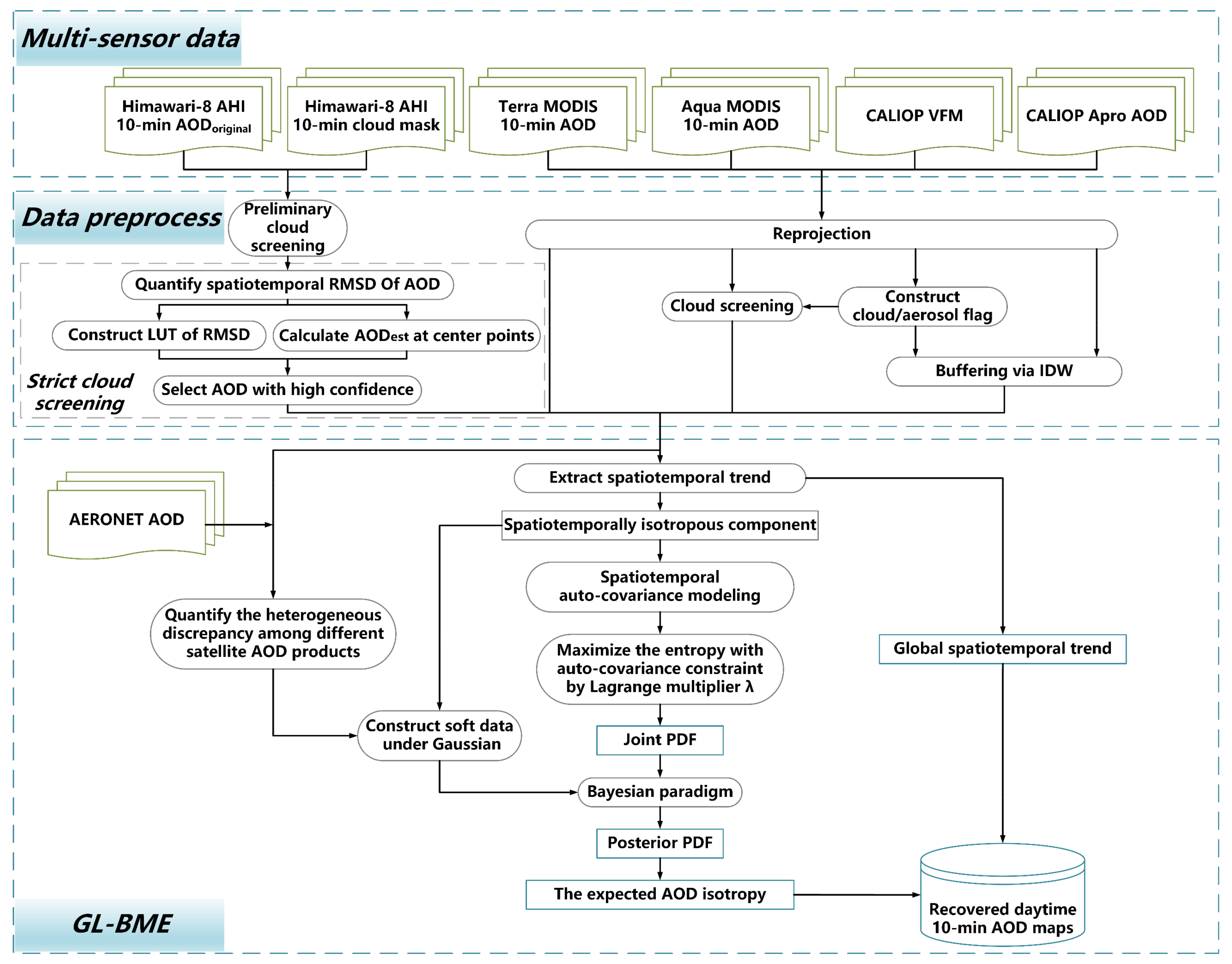
AERONET, a global network of calibrated sun photometers, can provide near-truth AOD measurements every 15 min at 340, 380, 440, 500, 670, 870, and 1020 nm wavelengths with an expected uncertainty of approximately 0.01 to 0.02 [54]. In this study, AERONET Level 2.0 (cloud-screened and quality-assured) version 3.0 AOD (Washington, DC, USA) measurements from 22 observation sites are adopted to serve as a reference for accuracy comparison between the satellite-based AOD retrievals and merged AODs. It is also used to quantify the discrepancy among satellite-based AOD products. MAN is mainly a periodical marine aerosol observation network using handheld Microtops II sun photometers on research vessel ships. MAN Level 2.0 AOD measurements are employed as a complementary part of the AERONET AOD over islands and oceans. It is notable that MAN measurements are often taken irregularly in time lags that vary with location and are of similar uncertainty (<0.02) to that of AERONET [55]. The aforementioned datasets are released on the website http://aeronet.gsfc.nasa.gov (accessed on 5 March 2022). The valid ground-based sites of AERONET and MAN are shown in Figure 1, and the elevation and geographic location are listed in Supporting Information Tables S1 and S2.

3. Methodology

The GL-BME fusion framework blending LEO and GEO satellite observations based on the Bayesian maximum entropy theorem is a pixel-based algorithm to recover the missing values with ensured accuracy in 10-min Himawari-8 AHI AOD images via incorporating discrepancies from different categories of products. As depicted in the flowchart in Figure 2, the GL-BME fusion framework is divided into two stages: (1) data preprocessing, in which multi-source satellite-based AOD products undergo a series of preprocesses, including space/time matching, quality control, and data combination, to ensure the spatiotemporal consistency and accuracy reliability of different AOD products; and (2) GL-BME fusion, in which the quality-assured AODs are blended based on the temporal and spatial autocorrelations to fill the data gaps, including constructing soft data under Gaussian distribution, modeling spatiotemporal covariance, estimating AOD isotropous component via the Bayesian paradigm, and adding global spatiotemporal trends to expected AOD isotropous components. More details on AOD fusion procedures and mathematical mechanisms are described in the following sections.

3.1. Data Preprocessing

The estimation accuracy of the merged AOD data largely depends on the quality of the input satellite-based AOD observations during the fusion process. To dispose of near-cloud contamination for AOD data with ensured reliability, the Himawari-8 AHI AOD retrievals after preliminary cloud screening (i.e., AOD_ori) further underwent strict quality control according to the AHI official L3 AOD algorithm [14]. For a center point $\left(x_0,y_0,t_0\right)$, the spatiotemporal variability at neighboring locations $\left(x_i,y_i,t_i\right)$ is quantified by the root mean square difference (RMSE) as follows:

$$\mathsf{\sigma }\left(∆L,∆t\right)=\sqrt{\frac{1}{N}{{\displaystyle \sum }}_1^N{\left(AO{D}_{ori}\left(x_i,y_i,t_i\right)-AO{D}_{ori}\left(x_0,y_0,t_0\right)\right)}^2}$$

(1)

where N is the total number of valid pixels within the calculation domain, ΔL = (($x_i$ − $x_0$)² + ($y_i$ − $y_0$)²)^1/2, and Δt = $t_i$ − $t_0$. Based on the corresponding AOD pairs at domain radius from 0 to 12.5 km and time ranges from 0 to 50 min, we establish the look-up-table (LUT) (seen in Supplementary Table S4) for $\mathsf{\sigma }\left(∆L,∆t\right)$. The estimated AOD at the center point, namely, $AO{D}_{est}\left(x_0,y_0,t_0\right)$, is interpolated from the AODs in a radius of 12.5 km and past of 1 h (except center point) with the inverse of their error variances as weights. It is expressed as follows:

$$AO{D}_{est}\left(x_0,y_0,t_0\right)={{\displaystyle \sum }}_{i=1}^N\frac{\frac{1}{{\sigma }_{ori}{\left(x_i,y_i,t_i\right)}^2}}{{{\displaystyle \sum }}_{i=1}^N\frac{1}{{\sigma }_{ori}{\left(x_i,y_i,t_i\right)}^2}}AO{D}_{ori}\left(x_i,y_i,t_i\right)$$

(2)

According to the joint Equations (3) and (4), $AO{D}_{pure}\left(x_0,y_0,t_0\right)$, the initial AHI AOD for the fusion process, is obtained from the $AO{D}_{ori}\left(x_0,y_0,t_0\right)$ if $AO{D}_{ori}\left(x_0,y_0,t_0\right)$ is within 2.58 ${\sigma }_{pure}\left(x_0,y_0,t_0\right)$ (i.e., the upper limit of the 99% confidence interval) based on the estimation of $AO{D}_{est}\left(x_0,y_0,t_0\right)$; otherwise, $AO{D}_{ori}\left(x_0,y_0,t_0\right)$ largely deviated from $AO{D}_{est}\left(x_0,y_0,t_0\right)$ is assigned to be a missing value due to near-cloud contamination. The $\sigma {\left(x_0,y_0,t_0\right)}^2$ at the center point is estimated via applying quadratic fitting in space and time of $\sigma {\left(∆L,∆t\right)}^2$.

$$AO{D}_{pure}\left(x_0,y_0,t_0\right)=\left\{\begin{array}{c} AO{D}_{ori}\left(x_0,y_0,t_0\right) if AO{D}_{ori}\left(x_0,y_0,t_0\right) \le AO{D}_{est}\left(x_0,y_0,t_0\right)+2.58{\sigma }_{pure}\left(x_0,y_0,t_0\right)\\ \mathit{\text{missing}} \mathit{\text{value}}\hspace{1em}\mathit{\text{else}}\hfill \end{array}\right.$$

(3)

$${\sigma }_{pure}\left(x_0,y_0,t_0\right)=\sqrt{\sigma {\left(x_0,y_0,t_0\right)}^2+{\sigma }_{est}{\left(x_0,y_0,t_0\right)}^2}$$

(4)

To match up other satellite-based AODs with Himawari-8 AHI AODs with a spatial resolution of 5 km, MODIS AOD, CALIOP AOD, and CALIOP cloud/aerosol identification flag are resampled into the same geographic girds as Himawari-8 AHI AOD using the cubic convolution interpolation method. Meanwhile, to compensate for the deficiency of CALIOP observations in spatial completeness, CALIOP datasets are expanded with a 40-km morphological buffer on both sides from the center of the original 5-km track based on inverse distance weighting (IDW) [51,56]. Benefiting from the similar scanning time and advantage of CALIOP in distinguishing clouds from aerosols, the dilated CALIOP cloud/aerosol identification flag is used to further screen Aqua MODIS AOD retrievals affected by cloud contamination. Similar to the strategies in our previous study [24], the cloud/aerosol identification grid will be set as a cloud flag if there exists any cloud flag pixel in interpolation and dilatation calculation since the potential abnormal AOD values contaminated by clouds should be excluded as much as possible to avoid error propagation in subsequent data fusion and recovery.

3.2. LEO/GEO-Integrated AOD Fusion Process

3.2.1. BME Method

The BME method is based on a knowledge processing framework with cognitive principles that can deal with the general knowledge base G (e.g., stochastic physical laws, empirical relationships, and scientific theories) and a specific knowledge base S (e.g., hard and soft data), which is beyond the reach of spatial statistics and linear geostatistics [57,58]. Hard data refers to data with accurate measurement or less error, while soft data generally has a certain degree of incompleteness or uncertainty. In this study, AOD observations provided by AERONET sites can be regarded as hard data, while AOD retrieved from satellite sensors could be regarded as soft data. The BME method contains three essential epistemological analysis stages: (1) the prior stage, (2) meta-prior stage, and (3) integration stage [59], which are briefly described as follows.

In the prior stage, the task is to obtain the joint probability density function (PDF) from G. For a vector of random variables x_map = [x_soft1, x_soft2…x_softm, x_k] at points x_soft1, x_soft2…x_softm with valid pixels and estimation point x_k with an invalid pixel, the expected information entropy function (Shannon’s information criterion) contained in the joint PDF of f_x(x_map) is defined by Equation (5):

$$H=-\int d{x}_{map}{f}_x\left(x_{map}\right)log{f}_x\left(x_{map}\right)$$

(5)

In general, when entropy is larger, that is, when there is more information, the probability distribution of the targeted random variables is more in tune with the actual situation [60,61]. The Lagrange multiplier λ_α is introduced to maximize entropy under the constraint of a set of functions of statistical spatiotemporal covariance moments (i.e., G), which is expressed as $g$_α(x_map) in this study [62]. The constructed function is expressed as follows:

$$F[x_{map},f_x\left(x_{map}),{\lambda }_{\alpha }\right]=-\int d{x}_{map}{f}_x\left(x_{map}\right)log{f}_x\left(x_{map}\right)-{{\displaystyle \sum }}_{\alpha =1}^N{\lambda }_{\alpha }\left[\int g_{\alpha }(x_{map})f_x\left(x_{map}\right)d{x}_{map}-g_{\alpha }\right]$$

(6)

where g_α denotes the mathematical expectation of $g$_α(x_map). By setting the first partial derivative with respect to x_map, f_x(x_map), and λ_α to zero, the joint PDF can then be solved using Equation (7):

$$f_x\left(x_{map}\right)=\frac{\exp \left[{{\displaystyle \sum }}_{\alpha =1}^N{\lambda }_{\alpha }{g}_{\alpha }(x_{map})\right]}{\int \exp \left[{{\displaystyle \sum }}_{\alpha =1}^N{\lambda }_{\alpha }{g}_{\alpha }(x_{map})\right]d{x}_{map}}$$

(7)

In the meta-prior stage, the task is to express S appropriately, which refers to the multi-source satellite-based AODs serving as soft data and are expressed as x_soft1, x_soft2…x_softm in this study. The construction process is described in detail in the following sections.

In the final integration stage, the posterior PDF can be obtained after updating the initial prior PDF by integrating G and S through operational Bayesian conditionalization [63], which is expressed as follows:

$$f\left(x_k|x_{soft1},x_{soft2}\dots x_{softm}\right)=\frac{f_x\left(x_{soft1},x_{soft2}\dots x_{softm},x_k\right)}{f_x\left(x_{soft1},x_{soft2}\dots x_{softm}\right)}=\frac{f_x\left(x_{map}\right)}{f_x\left(x_{soft1},x_{soft2}\dots x_{softm}\right)}$$

(8)

Finally, the nonlinear expected value at estimation point x_k is calculated using Equation (9):

$$\overline{x_k}=\int x_{k}f\left(x_k|x_{soft1},x_{soft2}\dots x_{softm}\right)d{x}_k$$

(9)

3.2.2. Soft Data Construction

Ground-based AOD observations acquired by AERONET and MAN are introduced to construct probabilistic soft data to reconcile the discrepancy from satellite-based AOD products, which is expressed as follows:

$$AO{D}_{sat,x,y,t}=AO{D}_{ground,x,y,t}+{\epsilon }_{x,y,t} \epsilon \sim N\left(\mu , {\sigma }^2\right)$$

(10)

where AOD_sat,x,y,t and AOD_ground,x,y,t are the satellite-based and AERONET or MAN AODs at the space–time coordinate (x, y, t), respectively, and the discrepancy ($\epsilon )$ approximately follows a normal distribution with mean (μ) and variance (σ²). Ground-based sites provide reduplicative point observations, whereas satellite observations provide images of a given area at a single time. Hence, to mitigate the influences of aerosol variability in space and time, the AOD values of the original satellite-based and merged data are extracted by spatially averaging 3 × 3 pixels (at least 20% valid pixels) centered at each ground-based site. Furthermore, the corresponding ground-based AODs are calculated by temporally averaging observations within ±30 min of the scanning time of each image [64]. Figure 3 depicts the Gaussian probability density functions of ε for satellite-based AODs, where the MODIS AOD product demonstrates the best data quality while the CALIOP AOD product generally possesses larger uncertainty than the MODIS and AHI AOD products due to the influences from surface reflection and sunlight [65,66,67,68]. For pixels where satellite-based AOD is valid, the Gaussian probability density soft data after discrepancy quantifying is expressed as follows:

$$AO{D}_{soft, sat }~N\left(AO{D}_{sat }+\mu , {\sigma }^2\right)$$

(11)

3.2.3. Spatiotemporal Covariance Modeling

For any variable Z(p) in the space/time random field (S/TRE), p = (s, t) denotes a spatiotemporal point (s is the geographic location, and t is time). It can be expressed using the following equation:

$$Z\left(p\right)=X\left(p\right)+m\left(p\right)$$

(12)

where the mean trend model X(p) is a function of parameter β. The zero-mean autocorrelated Gaussian process m(p) has covariance with parameter θ that varies at spatial lag γ = |s − s′| and temporal lag τ = |t − t′| (i.e., space/time distance between points p = (s, t) and p′= (s′, t′)). The fixed parameters β and θ can assist in describing the statistical distribution of variable Z [69]. In the BME method, all variables must be spatially homogenous and temporally stationary with constant mean and variance [70]. In this study, the spatiotemporal mean trend component is estimated and separated from the preprocessed satellite-based AOD datasets using a moving filter window of size 99 (pixels along-track) × 99 (pixels cross-track) × 3 (10 min). The remaining isotropic components are then employed to describe the spatiotemporal autocorrelation by modeling the covariance function. Figure 4a,b and

Table 2. Fitting results of the experimental covariance for the spatial and temporal lags based on three classical models (exponential, spherical, and Gaussian models).

Type/Parameters	Covariance vs. Spatial Lag			Covariance vs. Temporal Lag
	R2	RMB	RMSE	R2	SSE	RMSE
Exponential Model	0.94	1.110	0.0015	0.90	1.112	0.0016
Spherical Model	0.91	1.117	0.0017	0.86	1.116	0.0016
Gaussian Model	0.92	1.116	0.0016	0.82	1.114	0.0017

present the covariance modeling results for three theoretical fitting functions (i.e., exponential, spherical, and Gaussian models). It is demonstrated that the exponential fitting curve coincides the most with the experimental covariance, with the square of the Pearson correlation coefficient (R²) of 0.94 and 0.90, the relative mean bias (RMB) of 1.110 and 1.112, and the root-mean-square error (RMSE) of 0.0015 and 0.0016 under the condition of spatial lag and temporal lag, respectively. To sufficiently describe the sophisticated spatiotemporal variation process, we ultimately adopt the nested spatiotemporal covariance model with the superposition of two exponential functions [71,72]. Every model characterizes spatiotemporal dependency and is parameterized by partial sill variance ($c1$ or $c2$), spatial range (α_γ1 or α_γ2), and temporal range (α_τ1 or α_τ2):

$$C\left(\gamma ,\tau \right)=c1\mathit{exp}\left(-\frac{3\gamma }{a_{\gamma 1}}\right)\mathit{exp}\left(-\frac{3\tau }{a_{\tau 1}}\right)+c2\mathit{exp}\left(-\frac{3\gamma }{a_{\gamma 2}}\right)\mathit{exp}\left(-\frac{3\tau }{a_{\tau 2}}\right)$$

(13)

In this study, the interior point penalty function method is introduced to obtain the optimal parameter estimation of the above nested exponential models by constructing an unconstrained objective function as per our previous research [73]. Moreover, the nested spatiotemporal covariances are fitted for each month in this study due to the relatively large amount of 10-min AOD datasets to ensure the stability of the spatiotemporal covariance model and improve the efficiency of model fitting. Figure 4c shows a case of modeling the spatiotemporal covariance function over the study area. The parameter estimation results for every month during the study period are summarized in Supplementary Table S3.

4. Experimental Results and Analysis

4.1. Assessment of the Completeness of Merged AOD

A core objective of the GL-BME fusion framework is to maximally ameliorate the overall missing satellite-derived AOD products. Primarily, we quantitatively assess the spatial completeness of the original satellite-based and merged AOD datasets using the percentage of the number of pixels with valid AOD values over the experiment region. Figure 5 shows a comparison of the daily averaged AOD spatial completeness ratio among the original Himawari-8 AHI L2 AOD, merged AOD via only AHI AOD, and merged AOD via AHI, MODIS, and CALIOP AOD. The overall averaged spatial coverage of merged AOD after the GL-BME fusion process obviously improves from 20.3% to 67.6% compared to the original AOD. It can be found that the introduction of LEO sensors could additionally contribute to the spatial coverage improvement, approximately from 48.3% to 67.5%, which indicates that the introduction of LEO satellite sensors into the GL-BME fusion algorithm could further enhance the spatial completeness of the merged AOD. Moreover, the spatial completeness of the merged AOD exceeds 65% for almost half of the experimental period and even reaches up to 80% in a few days. The spatial distributions of annually averaged completeness for the original Himawari-8 AHI AOD data and merged AOD data are presented for comparison in Figure 6. As depicted in Figure 6a,b, the annually averaged completeness of the original AHI AOD data ranges from 0 to 39.2% with a median of 20.1%, whereas the annually averaged completeness of merged AOD data ranges from 41.3% to 98.2% with a median of 65.1%. Remarkably, the annually averaged completeness of the original Himawari-8 AHI AODs and merged AODs follows a consistent spatial variability pattern; that is, the coverage ratio is lowest in the southwest plateau region, followed by some high-latitude areas. As demonstrated in Figure 6c, there exists substantial improvement in the AOD completeness in the experimental regions, especially in the south of Mongolia and north of China, far from the Himawari-8 satellite nadir. The probable reason is that the original AHI AOD products periodically have intrinsic data blanks over these regions due to the combination of large viewing zenith and high surface reflectance, which could be well recovered by complementary AOD observations derived from LEO satellites.

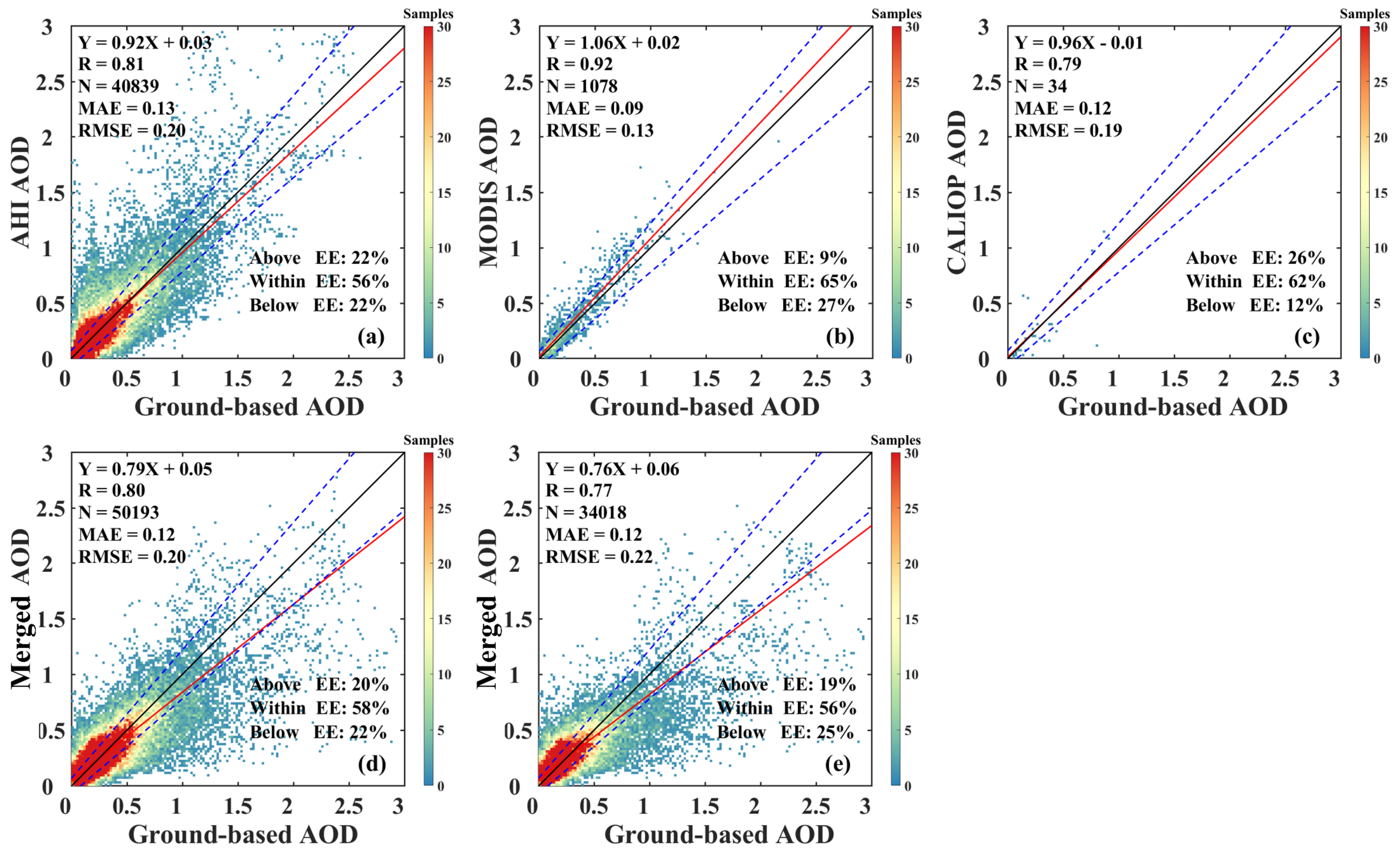
4.2. Accuracy Evaluation for Merged AOD

Another primary objective of the GL-BME fusion algorithm is to achieve high-quality merged AOD products. AERONET and MAN AOD observations are adopted to validate the merged AOD products and compare the accuracy between the merged AODs and original satellite-based AODs. The accuracy is quantitatively assessed by utilizing a set of evaluation metrics for statistical analysis, including the Pearson correlation coefficient (R), root-mean-square error (RMSE), mean absolute error (MAE), and expected error (EE) envelope combined with underestimation and overestimation ratios. The spatiotemporal matching strategy between all the satellite-based AODs and ground-based AODs is the same as the strategy mentioned in Section 3.2.2.

Figure 7 shows the validation results of the original satellite-based and merged AOD datasets against AERONET and MAN AOD observations over the whole experiment region during 2017. As shown in Figure 7a–c, the R, MAE, RMSE, above EE, within EE, and below EE based on 40,839 matchups from the original AHI AODs are 0.81, 0.13, 0.20, 22%, 56%, and 22%, respectively. For the 1078 matchups from the MODIS AODs, the R, MAE, RMSE, above EE, within EE, and below EE are 0.92, 0.09, 0.13, 9%, 65%, and 27%, respectively. For the 34 matchups from the CALIOP AOD datasets, the R, MAE, RMSE, above EE, within EE, and below EE are 0.79, 0.12, 0.19, 26%, 62%, and 22%, respectively. Figure 7d shows the overall accuracy of the merged AOD datasets over the whole experimental period and domain. The R, MAE, RMSE, above EE, within EE, and below EE based on 40,839 matchups are 0.80, 0.12, 0.20, 20%, 58%, and 22%, respectively. Additionally, Figure 7e demonstrates the accuracy of the merged AODs over areas where the initial AHI AODs are missing, with an R of 0.77 and approximately 56% of 34,018 matchups falling within the EE envelope. Moreover, the number of matchups below the EE envelope is higher than those above the EE envelope, with the underestimation mostly occurring at high aerosol loadings of >0.8. This is possibly due to the strict quality control process removing the cloud-influenced anomalies accompanied by the screening of some of the truly high AOD values. Admittedly, the comparison among Figure 7a,d,e demonstrates there exists a slight decrease in the accuracy of the merged AOD compared to the accuracy of the original AHI AOD, which is probably caused by AOD expectation estimation tending to be affected by spatiotemporally adjacent potential low AOD values and strict cloud screening preprocess to exclude some high AOD values to a certain extent. Overall, the merged AODs possess a relatively higher ratio within the EE envelop than the original AHI AODs, which indicates that the GL-BME fusion process could ensure the accuracy of the merged AOD dataset on the basis of dramatically enhancing the spatial coverage.

4.3. Error Analysis and Performance of AOD Fusion

Four-moment cases from different seasons are selected, in which the valid AOD pixels from the original Himawari-8 AHI possessed diverse spatial distributions to explore the AOD fusion details of the GL-BME. Figure 8a,b illustrates that there are data blanks in the original Himawari-8 AHI AOD, with the spatial coverage ranging from 27.3% to 34.2%. In contrast, the spatial coverage of the merged AOD datasets shows significant improvements, even up to 90% or more, which provide the possibility for spatiotemporally continuous analysis of aerosols. As shown in the third line of Figure 8, the estimation error variance (EEV) is adopted to evaluate the reliability of AOD expectation in the BME estimation. The EEV characterizes the estimation variance of the GL-BME fusion framework, which is calculated based on the number of available AODs within a certain spatiotemporal range centered at an estimated AOD pixel in the original satellite data as well as their spatiotemporal correlations. To be specific, when the original AOD is available, no fusion process is performed, and the EEV is 0 by default in this situation, and the EEV is updated along with the BME fusion process only when the original AOD is not available. Accordingly, the unreliable AOD estimations recovered by the GL-BME fusion algorithm are further excluded when the corresponding EEV is over 0.03 in this study, which are illustrated as blank areas in the second line of Figure 8. From the four selected moments throughout the experiment region, the highest EEV occurs over areas where there are not sufficient spatiotemporally adjacent AOD pixels, while the lowest EEV appears over areas where there exist enough valid adjacent AOD pixels in the original Himawari-8 AHI AOD with uniform spatiotemporal correlations.

Additionally, a comparison between the spatial distribution of the monthly merged AOD and monthly original L2 AHI AOD is conducted to further demonstrate the performance of the proposed GL-BME fusion process in restoring the real aerosol loading information. As illustrated in Figure 9, there remains a number of data blanks in the monthly averaged original AHI AOD maps, whereas the monthly averaged merged AOD maps after GL-BME fusion achieve complete coverage in each month. Furthermore, there are some specific improvements. First, sporadic noises with extremely high values caused by thin clouds or cloud edges are mixed with normal pixels in the original datasets, inevitably leading to an overestimation of the local pollution levels. The quality control strategy in this study screens these abnormal points during the fusion process, thus enabling the merged AOD to characterize the regional features of aerosols more accurately and stably. Second, the original AOD values are abnormally high in the immediate offshore area, wherein sediment is prone to accumulate, such as the sea areas near the Yangtze River Delta. In contrast, the merged AOD mitigates the excessive overestimation to a certain extent in individual months, particularly in August, September, and December. Third, the GL-BME fusion framework recovers the AOD values of the areas with relatively low aerosol loadings, such as the ocean and rural areas. Furthermore, there exist significant differences in some regions between the merged AOD and the original AHI AOD. For instance, it recovers relatively high values in heavily polluted areas (e.g., Beijing–Tianjin–Hebei region), obviously in January, February, March, and July. According to the comparisons of monthly averaged AOD among the ground-based AERONET AOD measurements, original and merged satellite-based AOD observations centered on two AERONET stations in Beijing (listed in Supplementary Table S5), the GL-BME fusion algorithm significantly increases the valid AOD observation days over Beijing in these months. Moreover, the ground-measured PM₁₀ concentrations in Beijing are adopted to supplementarily explain the reasonability of these recovered relatively high AOD values in the merged AOD dataset by comparing the variation trends of the monthly averaged satellite-based AODs and PM₁₀ throughout the year (seen in Supplementary Figure S1). It is demonstrated that the variation trends of monthly averaged merged AOD and monthly averaged PM₁₀ concentrations present a generally good consistency in Beijing during the experimental period. At the same time, the monthly averaged original AHI AOD demonstrates an obvious underestimation of the severity of atmospheric pollution in these months. Therefore, it is proven that the merged AOD after the GL-BME fusion could better characterize the real atmospheric pollution situation than the original AHI AOD product.

5. Conclusions

The data blanks in the geostationary satellite AOD products constrain its advantage and application in continuous monitoring of atmospheric aerosols with high frequency to a certain extent. In this study, we develop a spatiotemporal fusion framework maximally excavating the complementary advantages of LEO and GEO satellite sensors to obtain the Himawari-8 AHI 10-min AOD dataset with higher spatiotemporal coverage and desired accuracy. The proposed framework is a pixel-based AOD fusion algorithm on the moving windows of Himawari-8 AOD guided by the Bayesian maximum entropy theorem, combined with incorporating the discrepancies from different categories of products. The overall averaged spatial completeness of the merged AOD after GL-BME fusion significantly improves with an increment of nearly 50% (from 20.3% to 67.6%) over the original AHI AOD product and increases by nearly 20% than merged AOD via only AHI AOD, which shows the contribution of LEO to enhancing the performance of the merged AOD to a certain extent. The accuracy validation against AERONET and MAN AOD observations shows that there exists a slight decrease in the accuracy of the merged AOD compared to the accuracy of the original AHI AOD, yet the merged AODs possess a relatively higher ratio within the EE envelop than the original AHI AODs. Moreover, an estimation error variance analysis of the merged AOD for different moments indicates that the merged AODs via GL-BME fusion have sufficient reliability for aerosol-related applications, such as the assessment of aerosol radiation effects and their interaction with clouds. Furthermore, a comparison of the monthly averaged AOD maps between the original AHI AOD and merged AOD products shows that the merged AOD after the GL-BME fusion could better characterize the real atmospheric pollution situation than the original AHI AOD.

Since the quality of CALIOP data after 2017 is heavily influenced by low-energy laser shots, we accordingly adopt 2017 as the most recent study period and as a representative to evaluate the feasibility and performance of the GL-BME AOD fusion framework. Obviously, the proposed GL-BME fusion framework is also applicable to other geostationary satellites (e.g., the FY-4A and GOES-R series) and other years to substantially improve the availability of GEO satellite AOD products. Theoretically speaking, the merged AOD products could provide more spatiotemporally continuous information on aerosols, which is of practical significance for extensive atmospheric research and applications.

References

1. Lin, J.T.; Van Donkelaar, A.; Xin, J.Y.; Che, H.Z.; Wang, Y.S. Clear-sky aerosol optical depth over East China estimated from visibility measurements and chemical transport modeling. Atmos. Environ. 2014, 95, 258–267. [Google Scholar] [CrossRef]
2. Stocker, T.F.; Qin, D.; Plattner, G.K.; Tignor, M.M.B.; Allen, S.K.; Boschung, J.; Midgley, P.M. Contribution of working group I to the fifth assessment report of the intergovernmental panel on climate change. Clim. Chang. 2013, 5, 1–1552. [Google Scholar]
3. Sherman, J.P.; Sheridan, P.J.; Ogren, J.A.; Andrews, E.; Hageman, D.; Schmeisser, L.; Sharma, S.A. multi-year study of lower tropospheric aerosol variability and systematic relationships from four North American regions. Atmos. Chem. Phys. 2015, 15, 12487–12517. [Google Scholar] [CrossRef] [Green Version]
4. Zhang, T.; Zeng, C.; Gong, W.; Wang, L.; Sun, K.; Shen, H.; Zhu, Z. Improving spatial coverage for aqua MODIS AOD using NDVI-based multi-temporal regression analysis. Remote Sens. 2017, 9, 340. [Google Scholar] [CrossRef] [Green Version]
5. Anderson, T.L.; Charlson, R.J.; Bellouin, N.; Boucher, O.; Chin, M.; Christopher, S.A.; Haywood, J.; Kaufman, Y.J.; Kinne, S.; Ogren, J.A. An “a-train” strategy for quantifying direct climate forcing by anthropogenic aerosols. Bull. Am. Meteorol. Soc. 2005, 86, 1795. [Google Scholar] [CrossRef]
6. Barnaba, F.; Gobbi, G.P. Aerosol seasonal variability over the Mediterranean region and relative impact of maritime, continental and Saharan dust particles over the basin from MODIS data in the year 2001. Atmos. Chem. Phys. 2014, 4, 2367–2391. [Google Scholar] [CrossRef] [Green Version]
7. Pappas, V.; Hatzianastassiou, N.; Papadimas, C.; Matsoukas, C.; Kinne, S.; Vardavas, I. Evaluation of spatio-temporal variability of Hamburg Aerosol Climatology against aerosol datasets from MODIS and CALIOP. Atmos. Chem. Phys. 2013, 13, 8381–8399. [Google Scholar] [CrossRef] [Green Version]
8. Alexandrov, M.D.; Geogdzhayev, I.V.; Tsigaridis, K.; Marshak, A.; Levy, R.; Cairns, B. New statistical model for variability of aerosol optical thickness: Theory and application to MODIS data over ocean. J. Atmos. Sci. 2016, 73, 821–837. [Google Scholar] [CrossRef]
9. Abuelgasim, A.; Bilal, M.; Alfaki, I.A. Spatiotemporal variations and long term trends analysis of aerosol optical depth over the United Arab Emirates. Remote Sens. Appl. 2021, 23, 100532. [Google Scholar] [CrossRef]
10. Dubovik, O.; Schuster, G.L.; Xu, F.; Hu, Y.; Bösch, H.; Landgraf, J.; Li, Z. Grand challenges in satellite remote sensing. Front. Remote Sens. 2021, 2, 619818. [Google Scholar] [CrossRef]
11. Xie, Y.; Xue, Y.; Guang, J.; Mei, L.; She, L.; Li, Y.; Fan, C. Deriving a global and hourly data set of aerosol optical depth over land using data from four geostationary satellites: GOES-16, MSG-1, MSG-4, and Himawari-8. IEEE Trans. Geosci. Remote Sens. 2019, 58, 1538–1549. [Google Scholar] [CrossRef]
12. Chen, T.; Li, Z.; Kahn, R.A.; Zhao, C.; Rosenfeld, D.; Guo, J.; Chen, D. Potential impact of aerosols on convective clouds revealed by Himawari-8 observations over different terrain types in eastern China. Atmos. Chem. Phys. 2021, 21, 6199–6220. [Google Scholar] [CrossRef]
13. Andreae, M.O.; Rosenfeld, D.J. Aerosol–cloud–precipitation interactions. Part 1. The nature and sources of cloud-active aerosols. Earth-Sci. Rev. 2008, 89, 13–41. [Google Scholar] [CrossRef]
14. Kikuchi, M.; Murakami, H.; Suzuki, K.; Nagao, T.M.; Higurashi, A. Improved Hourly Estimates of Aerosol Optical Thickness Using Spatiotemporal Variability Derived from Himawari-8 Geostationary Satellite. IEEE Trans. Geosci. Remote Sens. 2018, 56, 3442–3455. [Google Scholar] [CrossRef]
15. Okuyama, A.; Andou, A.; Date, K.; Hoasaka, K.; Mori, N.; Murata, H.; Bessho, K. Preliminary validation of Himawari-8/AHI navigation and calibration. Earth Obs. Syst. XX 2015, 9607, 663–672. [Google Scholar]
16. Xia, X.; Min, J.; Wang, Y.; Shen, F.; Yang, C.; Sun, Z. Assimilating Himawari-8 AHI aerosol observations with a rapid-update data assimilation system. Atmos. Environ. 2019, 215, 116866. [Google Scholar] [CrossRef]
17. Lim, H.; Go, S.; Kim, J.; Choi, M.; Lee, S.; Song, C.K.; Kasai, Y. Integration of GOCI and AHI Yonsei aerosol optical depth products during the 2016 KORUS-AQ and 2018 EMeRGe campaigns. Atmos. Meas. Tech. 2021, 14, 4575–4592. [Google Scholar] [CrossRef]
18. Lippmann, M.; Ito, K.; Nadas, A.; Burnett, R.T. Association of particulate matter components with daily mortality and morbidity in urban populations. Res. Rep. Health Eff. Inst. 2000, 95, 5–72. [Google Scholar]
19. Tzanis, C.; Varotsos, C.; Christodoulakis, J.; Tidblad, J.; Ferm, M.; Ionescu, A.; Lefevre, R.A.; Theodorakopoulou, K.; Kreislova, K. On the corrosion and soiling effects on materials by air pollution in Athens, Greece. Atmos. Chem. Phys. 2011, 11, 12039–12048. [Google Scholar] [CrossRef] [Green Version]
20. Varotsos, C.; Ondov, J.; Tzanis, C.; Öztürk, F.; Nelson, M.; Ke, H.; Christodoulakis, J. An observational study of the atmospheric ultra-fine particle dynamics. Atmos. Environ. 2012, 59, 312–319. [Google Scholar] [CrossRef]
21. Carrer, D.; Ceamanos, X.; Six, B.; Roujean, J.L. AERUS-GEO: A newly available satellite-derived aerosol optical depth product over Europe and Africa. Geophys. Res. Lett. 2014, 41, 7731–7738. [Google Scholar] [CrossRef]
22. Ceamanos, X.; Six, B.; Riedi, J. Quasi-Global Maps of Daily Aerosol Optical Depth from a Ring of Five Geostationary Meteorological Satellites Using AERUS-GEO. J. Geophys. Res. Atmos. 2021, 126, 20. [Google Scholar] [CrossRef]
23. Lee, S.; Song, C.H.; Park, R.S.; Park, M.E.; Han, K.M.; Kim, J.; Woo, J.H. GIST-PM-Asia v1: Development of a numerical system to improve particulate matter forecasts in South Korea using geostationary satellite-retrieved aerosol optical data over Northeast Asia. Geosci. Model Dev. 2016, 9, 17–39. [Google Scholar] [CrossRef] [Green Version]
24. Xia, X.; Zhao, B.; Zhang, T.; Wang, L.; Gu, Y.; Liou, K.N.; Zhu, Z. Satellite-Derived Aerosol Optical Depth Fusion Combining Active and Passive Remote Sensing Based on Bayesian Maximum Entropy. IEEE Trans. Geosci. Remote Sens. 2021, 60, 1–13. [Google Scholar] [CrossRef]
25. Abdou, W.A.; Diner, D.J.; Martonchik, J.V.; Bruegge, C.J.; Kahn, R.A.; Gaitley, B.J.; Crean, K.A.; Remer, L.A.; Holben, B. Comparison of coincident MISR and MODIS aerosol optical depths over land and oceans scenes containing AERONET sites. J. Geophys. Res. 2005, 110, D10S07. [Google Scholar]
26. Kacenelenbogen, M.; Vaughan, M.A.; Redemann, J.; Hoff, R.M.; Rogers, R.R.; Ferrare, R.A.; Russell, P.B.; Hostetler, C.A.; Hair, J.W.; Holben, B.N. An accuracy assessment of the CALIOP/CALIPSO version 2/version 3 daytime aerosol extinction product based on a detailed multi-sensor, multi-platform case study. J. Geophys. Res. Atmos. 2011, 11, 3981–4000. [Google Scholar] [CrossRef] [Green Version]
27. Schuster, G.L.; Vaughan, M.; MacDonnell, D.; Su, W.; Winker, D.; Dubrovik, O.; Lapyonok, T.; Trepte, C. Comparison of CALIPSO aerosol optical depth retrievals to AERONET measurements, and a climatology for the LIDAR ratio of dust. J. Atmos. Chem. Phys. 2012, 12, 7431–7452. [Google Scholar] [CrossRef] [Green Version]
28. Han, B.; Ding, H.; Ma, Y.; Gong, W. Improving Retrieval Accuracy for Aerosol Optical Depth by Fusion of Modis and Caliop Data. Improv. Teh. Vjesn. 2017, 24, 3. [Google Scholar]
29. Ahn, S.; Chung, S.R.; Oh, H.J.; Chung, C.Y. Composite Aerosol Optical Depth Mapping over Northeast Asia from GEO-LEO Satellite Observations. Remote Sens. 2021, 13, 1096. [Google Scholar] [CrossRef]
30. Wang, Y.; Yuan, Q.; Li, T.; Shen, H.; Zheng, L.; Zhang, L. Large-scale MODIS AOD products recovery: Spatial-temporal hybrid fusion considering aerosol variation mitigation. ISPRS J. Photogramm. 2019, 157, 1–12. [Google Scholar] [CrossRef]
31. Li, K.; Bai, K.; Li, Z.; Guo, J.; Chang, N.B. Synergistic data fusion of multimodal AOD and air quality data for near real-time full coverage air pollution assessment. J. Environ. Manag. 2022, 302, 114121. [Google Scholar] [CrossRef] [PubMed]
32. Xiao, Q.; Wang, Y.; Chang, H.H.; Meng, X.; Geng, G.; Lyapustin, A.; Liu, Y. Fullcoverage high-resolution daily PM2.5 estimation using MAIAC AOD in the Yangtze River Delta of China. Remote Sens. Environ. 2017, 199, 437–446. [Google Scholar] [CrossRef]
33. Zhang, R.; Di, B.; Luo, Y.; Deng, X.; Grieneisen, M.L.; Wang, Z.; Zhan, Y. A nonparametric approach to filling gaps in satellite-retrieved aerosol optical depth for estimating ambient PM2.5 levels. Environ. Pollut. 2018, 243, 998–1007. [Google Scholar] [CrossRef] [PubMed]
34. Zhao, C.; Liu, Z.; Wang, Q.; Ban, J.; Chen, N.X.; Li, T. High-resolution daily AOD estimated to full coverage using the random forest model approach in the BeijingTianjin-Hebei region. Atmos. Environ. 2019, 203, 70–78. [Google Scholar] [CrossRef]
35. Ali, A.; Amin, S.E.; Ramadan, H.H.; Tolba, M.F. Enhancement of OMI aerosol optical depth data assimilation using artificial neural network. Neural Comput. Appl. 2013, 23, 2267–2279. [Google Scholar] [CrossRef]
36. Bi, J.; Belle, J.H.; Wang, Y.; Lyapustin, A.I.; Wildani, A.; Liu, Y. Impacts of snow and cloud covers on satellite-derived PM2.5 levels. Remote Sens. Environ. 2018, 221, 665–674. [Google Scholar] [CrossRef]
37. Park, S.; Lee, J.; Im, J.; Song, C.K.; Choi, M.; Kim, J.; Lee, S.; Park, R.; Kim, S.M.; Yoon, J.; et al. Estimation of spatially continuous daytime particulate matter concentrations under all sky conditions through the synergistic use of satellite-based AOD and numerical models. Sci. Total Environ. 2020, 713, 136516. [Google Scholar] [CrossRef]
38. Jiang, T.; Chen, B.; Nie, Z.; Ren, Z.; Xu, B.; Tang, S. Estimation of hourly full coverage PM2.5 concentrations at 1-km resolution in China using a two-stage random forest model. Atmos. Res. 2021, 248, 105146. [Google Scholar] [CrossRef]
39. Lanzaco, B.L.; Olcese, L.E.; Palancar, G.G.; Toselli, B.M. A method to improve MODIS AOD values, Application to South America. Aerosol Air Qual. Res. 2016, 16, 1509–1522. [Google Scholar] [CrossRef] [Green Version]
40. Li, L.; Franklin, M.; Girguis, M.; Lurmann, F.; Wu, J.; Pavlovic, N.; Breton, C.; Gilliland, F.; Habre, R. Spatiotemporal imputation of MAIAC AOD using deep learning with downscaling. Remote Sens. Environ. 2020, 237, 111584. [Google Scholar] [CrossRef]
41. Chatterjee, A.; Michalak, A.M.; Kahn, R.A.; Paradise, S.R.; Braverman, A.J.; Miller, C.E. A geostatistical data fusion technique for merging remote sensing and ground-based observations of aerosol optical thickness. J. Geophys. Res. 2010, 115, D20207. [Google Scholar] [CrossRef] [Green Version]
42. Xu, H.; Guang, J.; Xue, Y.; de Leeuw, G.; Che, Y.H.; Guo, J.; He, X.W.; Wang, T.K. A consistent aerosol optical depth (AOD) dataset over mainland China by integration of several AOD products. Atmos. Environ. 2015, 114, 48–56. [Google Scholar] [CrossRef]
43. Yang, J.; Hu, M. Filling the missing data gaps of daily MODIS AOD using spatiotemporal interpolation. Sci. Total Environ. 2018, 633, 677–683. [Google Scholar] [CrossRef] [PubMed]
44. Gupta, P.; Patadia, F.; Christopher, S.A. Multisensor data product fusion for aerosol research. IEEE Trans. Geosci. Remote Sens. 2008, 46, 1407–1415. [Google Scholar] [CrossRef]
45. Wang, J.; Brown, D.G.; Hammerling, D. Geostatistical inverse modeling for super-resolution mapping of continuous spatial processes. Remote Sens. Environ. 2013, 139, 205–215. [Google Scholar] [CrossRef]
46. Nguyen, H.; Cressie, N.; Braverman, A. Spatial statistical data fusion for remote sensing applications. J. Am. Stat. Assoc. 2012, 107, 1004–1018. [Google Scholar] [CrossRef]
47. Puttaswamy, S.J.; Nguyen, H.M.; Braverman, A.; Hu, X.; Liu, Y. Statistical data fusion of multi-sensor AOD over the continental United States. Geocarto Int. 2013, 29, 48–64. [Google Scholar] [CrossRef]
48. Kokhanovsky, A.A.; Breon, F.M.; Cacciari, A.; Carboni, E.; Diner, D.; Di Nicolantonio, W.; von Hoyningen-Huene, W. Aerosol remote sensing over land: A comparison of satellite retrievals using different algorithms and instruments. Atmos. Res. 2007, 85, 372–394. [Google Scholar] [CrossRef]
49. Tang, Q.; Bo, Y.; Zhu, Y. Spatiotemporal fusion of multiple-satellite aerosol optical depth (AOD) products using Bayesian maximum entropy method. J. Geophys. Res. Atmos. 2016, 121, 4034–4048. [Google Scholar] [CrossRef] [Green Version]
50. CALIPSO Low Laser Energy Technical Advisory for Data Users. Available online: https://www-calipso.larc.nasa.gov/resources/calipso_users_guide/advisory/advisory_2018-10-10-CALIPSO_Laser_Energy_Technical_Advisory_Ver03 (accessed on 20 March 2022).
51. Campbell, J.R.; Tackett, J.L.; Reid, J.S.; Zhang, J.; Curtis, C.A.; Hyer, E.J.; Winker, D.M. Evaluating nighttime CALIOP 0.532 μm aerosol optical depth and extinction coefficient retrievals. Atmos. Meas. Tech. 2012, 5, 2143–2160. [Google Scholar] [CrossRef] [Green Version]
52. Vaughan, M.A.; Powell, K.A.; Winker, D.M.; Hostetler, C.A.; Kuehn, R.E.; Hunt, W.H.; McGill, M.J. Fully automated detection of cloud and aerosol layers in the CALIPSO lidar measurements. J. Atmos. Ocean. Tech. 2009, 26, 2034–2050. [Google Scholar] [CrossRef]
53. Liu, Z.; Winker, D.; Omar, A.; Vaughan, M.; Trepte, C.; Hu, Y.; Lin, B. Effective lidar ratios of dense dust layers over North Africa derived from the CALIOP measurements. J. Quant. Spectrosc. Ra. 2011, 112, 204–213. [Google Scholar] [CrossRef]
54. Eck, T.F.; Holben, B.N.; Reid, J.S.; Dubovik, O.; Smirnov, A.; O’neill, N.T.; Kinne, S. Wavelength dependence of the optical depth of biomass burning, urban, and desert dust aerosols. J. Geophys. Res. Atmos. 1999, 104, 31333–31349. [Google Scholar] [CrossRef]
55. Smirnov, A.; Holben, B.N.; Slutsker, I.; Giles, D.M.; McClain, C.R.; Eck, T.F.; Jourdin, F. Maritime aerosol network as a component of aerosol robotic network. J. Geophys. Res. Atmos. 2009, 114, D6. [Google Scholar] [CrossRef] [Green Version]
56. Omar, A.H.; Winker, D.M.; Tackett, J.L.; Giles, D.M.; Kar, J.; Liu, Z.; Trepte, C.R. CALIOP and AERONET aerosol optical depth comparisons: One size fits none. J. Geophys. Res. Atmos. 2013, 118, 4748–4766. [Google Scholar] [CrossRef]
57. Akita, Y.; Chen, J.C.; Serre, M.L. The moving-window Bayesian maximum entropy framework: Estimation of PM (2.5) yearly average concentration across the contiguous United States. J. Exposure Sci. Environ. Epidemiol. 2012, 22, 496–501. [Google Scholar] [CrossRef] [Green Version]
58. Christakos, G.; Li, X. Bayesian maximum entropy analysis and mapping: A farewell to kriging estimators? Math. Geol. 1998, 30, 435–462. [Google Scholar] [CrossRef]
59. Nazelle, A.D.; Arunachalam, S.; Serre, M.L. Bayesian maximum entropy integration of ozone observations and model predictions: An application for attainment demonstration in North Carolina. Environ. Sci. Technol. 2010, 44, 5707–5713. [Google Scholar] [CrossRef] [Green Version]
60. Jaynes, E.T. Information theory and statistical mechanics. Phys. Rev. 1957, 106, 620–630. [Google Scholar] [CrossRef]
61. Jaynes, E.T. Notes on Present Status and Future Prospects. In Fundamental Theories of Physics; Springer: Dordrecht, The Netherlands, 1990; pp. 1–13. [Google Scholar]
62. Holben, B.N.; Eck, T.F.; Slutsker, I.A.; Tanre, D.; Buis, J.P.; Setzer, A.; Smirnov, A. AERONET—A federated instrument network and data archive for aerosol characterization. Remote Sens. Environ. 1998, 66, 1–16. [Google Scholar] [CrossRef]
63. Spadavecchia, L.; Williams, M. Can spatio-temporal geostatistical methods improve high resolution regionalisation of meteorological variables? Agricult. Forest Meteorol. 2009, 149, 1105–1117. [Google Scholar] [CrossRef]
64. Bilal, M.; Nichol, J.E. Evaluation of MODIS aerosol retrieval algorithms over the Beijing-Tianjin-Hebei region during low to very high pollution events. J. Geophys. Res-Atmos. 2015, 120, 7941–7957. [Google Scholar] [CrossRef] [Green Version]
65. Huang, Y.; Zhu, B.; Zhu, Z.; Zhang, T.; Gong, W.; Ji, Y.; Xia, X.; Wang, L.; Zhou, X.; Chen, X. Evaluation and comparison of MODIS collection 6.1 and collection 6 dark target aerosol optical depth over mainland China under various conditions including spatiotemporal distribution, haze effects, and underlying surface. Earth Space Sci. 2019, 6, 2575–2592. [Google Scholar] [CrossRef] [Green Version]
66. Zhang, T.; Wang, L.; Zhao, B.; Gu, Y.; Wong, M.S.; She, L.; Xia, X.; Dong, J.; Ji, Y.; Gong, W.; et al. A Geometry-Discrete Minimum Reflectance Aerosol Retrieval Algorithm (GeoMRA) for Geostationary Meteorological Satellite Over Heterogeneous Surfaces. IEEE Trans. Geosci. Remote Sens. 2022, 60, 1–14. [Google Scholar] [CrossRef]
67. Gong, W.; Huang, Y.; Zhang, T.; Zhu, Z.; Ji, Y.; Xiang, H. Impact and suggestion of column-to-surface vertical correction scheme on the relationship between satellite AOD and ground-level PM2. 5 in China. Remote Sens. 2017, 9, 1038. [Google Scholar] [CrossRef] [Green Version]
68. Zhang, T.; Gong, W.; Zhu, Z.; Sun, K.; Huang, Y.; Ji, Y. Semi-physical estimates of national-scale PM10 concentrations in China using a satellite-based geographically weighted regression model. Atmosphere 2016, 7, 88. [Google Scholar] [CrossRef] [Green Version]
69. Brooker, P.I. A parametric study of robustness of kriging variance as a function of range and relative nugget effect for a spherical semivariogram. Math. Geol. 1986, 18, 477–488. [Google Scholar] [CrossRef]
70. Cressie, N.A.C. Statistics for Spatial Data; Wiley: New York, NY, USA, 1993. [Google Scholar]
71. Genton, M.G.; Gorsich, D.J. Variogram model selection via nonparametric derivative estimation. Math. Geol. 2000, 32, 249–270. [Google Scholar] [CrossRef]
72. Christakos, G. Modern Spatiotemporal Geostatistics; Oxford University Press: London, UK, 2000. [Google Scholar]
73. Shi, T.; Han, Z.; Gong, W.; Ma, X.; Han, G. High-precision methodology for quantifying gas point source emission. J. Clean. Prod. 2021, 320, 128672. [Google Scholar] [CrossRef]
Figure 1. Spatial distribution of 22 AERONET (red circles) and MAN (brown triangle) sites.
Remotesensing 15 02038 g001
Figure 2. Flowchart of the AOD fusion by integrating LEO and GEO AOD products. (RMSD and PDF are the abbreviations of root-mean-square difference and probability density function, respectively).
Remotesensing 15 02038 g002
Figure 3. Gaussian probability density functions of the random discrepancy between (a) Himawari-8 AHI AODs, (b) MODIS AODs, and (c) CALIOP and AERONET AODs.
Remotesensing 15 02038 g003
Figure 4. (a,b) Experimental (circles) and fitted theoretical (solid line) covariance shown as a function of the spatial lag (0 to 250 km) and the temporal lag, respectively. The exponential model fitting is shown as red solid line, the spherical model fitting is shown as blue solid line, and the green solid line represents the Gaussian model fitting. (c) Experimental (gray solid dots) and fitted nested theoretical spatiotemporal covariance (color). The spatial lag (0 to 250 km) is shown on the left axis, and the temporal lag (0 to 200 min) is shown on the right axis and the spatiotemporal covariance on the vertical axis. Experimental covariance is calculated from the point pairs at specific distances according to AOD datasets after spatiotemporal trend removal, which is based on datasets from May 2017.
Remotesensing 15 02038 g004
Figure 5. Daily averaged AOD spatial completeness ratio in 2017 for the original Himawari-8 AHI AOD (green), merged AOD blending AHI, MODIS, and CALIOP AOD based on GL-BME (red) and merged AOD via only AHI AOD based on BME (blue).
Remotesensing 15 02038 g005
Figure 6. Spatial distribution of the annually averaged coverage ratio in 2017 for the (a) original Himawari-8 L2 AHI AOD datasets and (b) merged AOD datasets after GL-BME fusion, combined with (c) coverage improvement from original AHI AOD to merged AOD.
Remotesensing 15 02038 g006
Figure 7. Validation results of the (a) original Himawari-8 L2 AHI, (b) MODIS, (c) CALIOP, (d) merged AODs, and (e) merged AODs s for areas where the initial Himawari-8 AHI, MODIS, and CALIOP AODs are all missing with AERONET and MAN AODs as benchmarks. The black, blue, and red lines represent the 1:1 reference, EE envelop, and regression lines of the AOD matchups, respectively.
Remotesensing 15 02038 g007
Figure 8. Maps of the original Himawari-8 AHI AOD (first line), merged AOD (second line), and estimation error variance (EEV) of the merged AOD data (third line) in the experimental region on 15 February, 25 May, 20 October, and 3 December of 2017.
Remotesensing 15 02038 g008
Figure 9. Maps of the monthly spatial distribution in 2017 for the original Himawari-8 L2 AHI and merged AOD datasets. The color bar represents the AOD values.
Remotesensing 15 02038 g009