Article

MTCSNet: Mean Teachers Cross-Supervision Network for Semi-Supervised Cloud Detection

1
State Key Laboratory of Information Engineering in Surveying, Mapping and Remote Sensing, Wuhan University, 129 Luoyu Road, Wuhan 430079, China
2
China Ship Development and Design Center, 268 Zhangzhidong Road, Wuhan 430064, China
*
Author to whom correspondence should be addressed.
Remote Sens. 2023, 15(8), 2040; https://doi.org/10.3390/rs15082040
Submission received: 7 March 2023 / Revised: 2 April 2023 / Accepted: 10 April 2023 / Published: 12 April 2023
(This article belongs to the Section AI Remote Sensing)

Abstract

:
Cloud detection methods based on deep learning depend on large and reliable training datasets to achieve high detection accuracy. There will be a significant impact on their performance, however when the training data are insufficient or when the label quality is low. Thus, to alleviate this problem, a semi-supervised cloud detection method, named the mean teacher cross-supervision cloud detection network (MTCSNet) is proposed. This method enforces both consistency and accuracy on two cloud detection student network branches, which are perturbed with different initializations, for the same input image. For each of the two student branches, the respective teacher branches, used to generate high-quality pseudo labels, are constructed using an exponential moving average method (EMA). A pseudo one-hot label, produced by one teacher network branch, supervises the other student network branch with the standard cross-entropy loss, and vice versa. To incorporate additional prior information into the model, the presented method uses near-infrared bands instead of red bands as model inputs and injects strong data augmentations on unlabeled images fed into the student model. This induces the model to learn richer representations and ensure consistency constraints on the predictions of the same unlabeled image across different batches. To attain a more refined equilibrium between the supervised and semi-supervised loss in the training process, the proposed cloud detection network learns the optimal weights based on homoscedastic uncertainty, thus effectively exploiting the advantages of semi-supervised tasks and elevating the overall performance. Experiments on the SPARCS and GF1-WHU public cloud detection datasets show that the proposed method outperforms several state-of-the-art semi-supervised algorithms when only a limited number of labeled samples are available.

1. Introduction

With the rapid development of Earth observation technologies, we now have access to a large number of optical remote sensing images collected daily, which provide rich information for surface observation. However, the presence of clouds remains one of the main factors affecting the quality of optical remote-sensing images due to the global average annual cloud coverage rate of 66% [1]. Cloud contamination not only limits the visibility and clarity of optical remote sensing images, but also affects the accuracy of subsequent surface observations and hence, application such as land use classification [2], change detection [3,4], and estimation of atmospheric variability estimation [5]. Therefore, the accurate detection of clouds is a key task in the Earth observation domain.
Many researchers have applied deep learning methods to cloud detection tasks with the development of deep learning technology. Compared with the cloud detection methods based on spectral thresholding, the deep learning-based methods do not need to manually design the feature extraction method, but let the deep learning models themselves learn the semantic information related to cloud detection from the spatial and spectral features of the input remote sensing imagery data through training data. Many researchers have already proposed algorithms related to cloud detection based on deep learning, including CNN (Convolutional Neural Network) [6,7,8,9,10,11,12,13,14,15,16,17], GAN (Generative Adversarial Network) [18,19], and Attention Mechanism [20,21,22]. Some researchers have also constructed deep learning models specifically for cloud snow detection through feature fusion modules, adding geographical prior information, such as Wu et al. [23], Chen et al. [24], Zhang et al. [25], and Guo et al. [20]. Some researchers have also studied the cross-domain problem between different remote-sensing images [26,27].
Although the accuracy of cloud detection can be significantly improved by introducing prior information or designing a different network structure, most of them rely heavily on training data. If the training data are insufficient (or unrepresentative) or the training labels are inaccurate, the model may have cognitive bias, which will affect the final performance.
However, obtaining a large number of high-quality cloud labels is a challenging and time-consuming task. For instance, Figure 1a illustrates that highly mixed scenes and uneven terrain can lead to indistinct boundaries between clouds and background features, particularly in the case of thin cloud layers [17]. Additionally, Figure 1b,c reveals that various scales of scattered and thin clouds are commonly seen. These complexities demonstrate the difficulty in accurately labeling clouds. According to the annotation work of the Cityscapes dataset [28], it usually takes more than one hour to label an urban scene image of 1024 × 2048 pixels. In fact, unlabeled remote sensing imagery data are abundant and can be effectively utilized by semi-supervised methods to assist model training. This reduces the demand for a large number of high-quality labeled samples and lowers the annotation workload. Consequently, semi-supervised cloud detection is of great significance in detecting clouds in remote sensing images.
Cloud detection based on semi-supervision is a sub-task of semi-supervised semantic segmentation. In recent years, two primary research branches have been proposed for semi-supervised semantic segmentation, namely entropy minimization and consistency regularization. Minimizing entropy, also known as self-training, uses pseudo segmentation labels on unlabeled data obtained from a model previously trained on labeled data to retrain the model [29,30,31]. This process can be iterated multiple times. Nambiar et al. [32] proposed a multi-stage self-training approach for performing the detection of cloud, shadow, and snow on Sentinel-2 L1C images. This approach utilizes the noisy Fmask labels for training and a small human-labeled dataset for validation. At each iterative stage, a larger network architecture is used in comparison to the previous stage, and a new model is trained. The trained model is then used to generate new training labels for a bigger dataset, which are used to train the model in the next stage. This approach can help avoid the negative impact of too many noisy labels in Fmask in the early training process, however, the problem of noisy labels in the first training phase is still not addressed.
Consistency regularization is another commonly used method for semi-supervised semantic segmentation. The fundamental concept of this approach is to incentivize the model to produce similar predictions for identical samples when subjected to varying transformations [33,34,35]. Common perturbation methods include input-level perturbation (feeding the model with strong augmentation and weaky augmentation unlabeled images and constraining the model to predict them consistently, represented by PseudoSeg [36]), feature-level perturbation (perturbing the features output from the encoder part of the model and then constraining the model decoder to decode similar prediction results for the features before and after the perturbation, represented by CCT [37]), and network level perturbation (inputting unlabeled images into two different networks and constraining these two networks to predict same unlabeled image with the same result, represented by the method CPS [38]). Guo et al. [39] introduced a semi-supervised cloud detection method called SSCDnet, which presents a feature-level and output-level domain adaptation approach to minimize the differences between the distribution of labeled and unlabeled images. Moreover, the generated pseudo label is filtered by a double-thresholded screening strategy based on feedback from the output-level domain adaptation, which ensures the selection of dependable regions.
Most of the aforementioned methods focus on maintaining consistency between the generated pseudo labels before and after the perturbation without emphasizing the accuracy of these pseudo labels. However, low-quality pseudo labels can induce cognitive bias in the model, leading to adverse effects. Furthermore, most current semi-supervised methods set a hyperparameter λ to balance a trade-off between the supervised part and the semi-supervised part, which has a significant impact on the model’s performance. The optimal value of this hyperparameter varies for different datasets or tasks, thus requiring a lot of effort and experiment to find its best-fit value. To address these issues, this paper proposes a novel and simple semi-supervised approach for cloud detection named MTCSNet. MTCSNet constructs teacher branches of the student branches through EMA (Exponential Moving Average), which helps generate more accurate and stable pseudo-labels. Inspired by multi-task learning using uncertainty to weigh losses [40], MTCSNet learns the optimal weights for both supervised and semi-supervised losses based on homoscedastic uncertainty, resulting in better learning from the unlabeled images.
In summary, the contributions of this paper are summarized as follows:
(i)
The MTCSNet replaces the cross-supervision between student branches with cross-supervision between teacher and student branches, providing more accurate and stable supervision signals to the student branch. Furthermore, strong data augmentation is applied to unlabeled images fed to the student branch, which introduces more prior information and enforces consistency constraints on the prediction results of the same unlabeled image across different batches. Additionally, near-infrared band is used instead of red band as input to assist model training.
(ii)
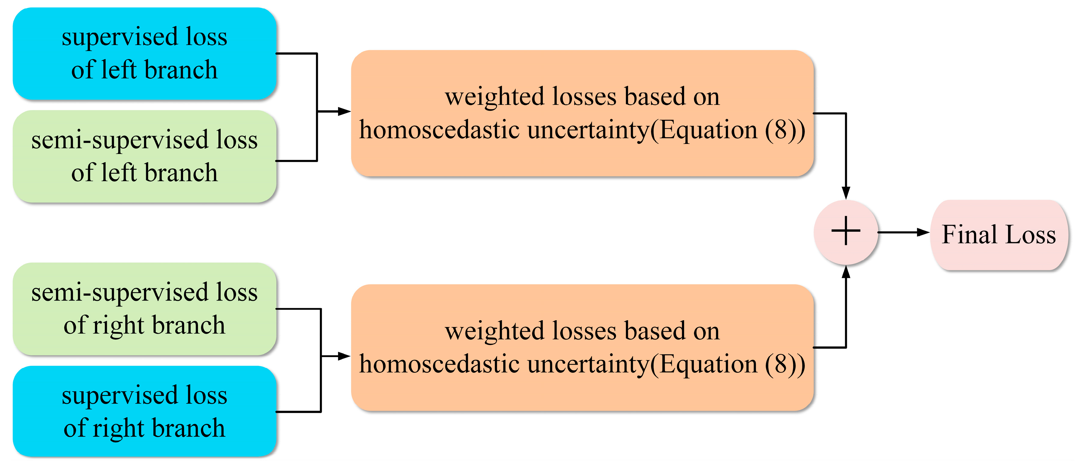
The MTCSNet learns the weights of supervised and semi-supervised losses based on homoscedastic uncertainty for improving model performance. The weights of supervised and semi-supervised losses are dynamically adjusted in every iteration instead of remaining constant. Losses with higher uncertainty will be assigned with smaller weights which results in a smoother and more effective training process. By avoiding fixed loss weights that drag on model performance, the proposed method can better benefit from both supervised and semi-supervised learning tasks. Details are introduced in Section 2.3.
(iii)
The effectiveness of the proposed method is verified on two cloud detection datasets. The results show that the proposed method can better utilize unlabeled data for learning and outperforms several state-of-the-art semi-supervised algorithms.

2. The Proposed Methods

The proposed MTCSNet comprises two student network branches that share the same structure, but differ in the way of initialization, as well as two teacher network branches that are created through EMA on student network branches. Additionally, near-infrared band is used instead of red band as input to the model. The proposed approach involves the feeding of both weakly augmented labeled and strongly augmented unlabeled images into two student network branches, while only the weakly augmented unlabeled images are fed into teacher network branches. The outputs of two student branches on labeled data are supervised independently by corresponding ground-truth labels. The output of left student branch for the weakly augmented labeled data and the strongly augmented unlabeled data are collectively referred to as the left pseudo segmentation map. This map is supervised using one-hot pseudo labels generated from the output of the right student branch for the weakly augmented labeled data and the output of the right teacher branch for the weakly augmented unlabeled data, respectively. It holds true for the right pseudo segmentation map likewise.
The process for calculating the loss can be summarized as follows: The supervised loss s u p l e f t is calculated based on the predicted results of the model’s left branch for labeled data and corresponding ground-truth labels. The semi-supervised loss u n s u p l e f t is calculated by the left pseudo segmentation map with pseudo labels from the right branch. Then, the comprehensive loss l e f t is calculated from s u p l e f t and u n s u p l e f t based on the homoscedastic uncertainty. Similarly, the loss r i g h t can be calculated for the right branch. Finally, the total loss t o t a l l y = l e f t + r i g h t is the sum of l e f t and r i g h t .

2.1. Motivation

The motivation for the proposed approach is derived from the following three aspects:
Consistency and accuracy: Most of the current methods constrain the prediction results before and after perturbation to be consistent, rather than consistent and correct at the same time. Once the predictions of unlabeled images are inaccurate, these imprecise pseudo-labels can introduce erroneous supervisory signals to the model, leading to confirmation bias and ultimate degrading consistency learning. Therefore, we construct teacher branches of student branches by EMA based on CPS. The teacher branches are used to generate high-quality and stable pseudo labels from unlabeled data. The pseudo label produced by one teacher network branch is utilized to supervise the other student network branch with the standard cross-entropy loss, and vice versa.
Moreover, to introduce more prior information into the model during the training process, strong data augmentations are performed for unlabeled images input to the student model and weak data augmentations for unlabeled images input to the teacher model. Considering that remote sensing images may be obtained from sensors with different resolutions, under different seasons, lighting, brightness conditions, etc., strong data augmentations are used including color jittering (randomly changing the brightness, contrast, and saturation of the image) and Gaussian blurring. In addition to spectral features, we also anticipate the model pays more attention to the texture features of clouds, so the input unlabeled images are turned into grayscale images with a probability of 0.2. Since the predictions output by the teacher branch are relatively accurate and stable, the predictions of the student model between different batches for the same unlabeled image subject to different strong data augmentation are also subject to the consistency regularity constraint.
Near-infrared band: Since the location of clouds is generally existent in the higher altitude region of the atmosphere, their temperature tends to be lower compared to other land covers. Additionally, water droplets and ice crystals presented in clouds scatter and absorb radiation in NIR band, which results in a higher reflectance in NIR band. Therefore, the features of clouds are more distinct in NIR band rather than in red band. As a result, in this study, NIR band is used as input to the model for training instead of red band.
Homoscedastic Uncertainty-based Loss Weighting (HULW): In most methods, a trade-off weight λ is set, which is an empirical value to assess the weights between supervised and semi-supervised losses, and the optimal λ needs to be re-explored once the dataset has transformed, or the method has improved, or even the proportion of labeled data has changed. Inspired by multi-task learning using uncertainty to weigh losses [40], the proposed method no longer uses a fixed value but uses homoscedastic uncertainty to measure the weight of supervised loss and semi-supervised loss, allowing the model to find an optimal weight during the training process, thus allowing the model to better balance supervised and semi-supervised tasks during training and achieve better performance.

2.2. MTCSNet Architecture

A novel semi-supervised cloud detection method named MTCSNet (Mean Teacher Cross-supervised Network) has been proposed, and its architecture is shown in Figure 2.
Before the proposed approach is introduced, relevant symbolic markers will be introduced first. The labeled training set is denoted by D L = x i , y i i = 1 | D L | , where x i X R H × W × C is the input remote sensing images of size H × W with C band channels, and y i Y 0 , 1 H × W × Y is the mask map, with the number of classes denoted by Y . The unlabeled training set is denoted by D U = x i i = 1 | D U | with | D L | | D U | . The total data set is denoted by D L & U = D L , D U .
As shown in Figure 2, MTCSNet has two branches and they have the same architecture, denoted by f θ : X R H × W × Y , where θ is the model parameter. The left branch is denoted by f θ l e f t s and the right branch is denoted by f θ r i g h t s . As mentioned in Section 2.1, to make the predictions of the left and right branches are consistent and correct, their respective teacher branches are constructed by the EMA of the student branches, denoted by f θ l e f t t and f θ r i g h t t , respectively. The whole model needs to be trained and optimized with parameters is denoted by θ s = θ l e f t s , θ r i g h t s .
The labeled image X l in Figure 2 is inputted to the left and right student branches of the network after weaky data augmentations, and the obtained output results are denoted by y ^ l e f t w e a k _ l and y ^ r i g h t w e a k _ l , respectively.
The unlabeled image X u in Figure 2 after weaky data augmentations is inputted to the left and right teacher branches of the network with gradient update stopped, and the obtained output results are denoted by y ^ l e f t w e a k _ u and y ^ r i g h t w e a k _ u , respectively. The unlabeled image X u in Figure 2 after strong data augmentations is inputted it to the left and right student branches of the network, and the obtained output results are denoted by y ^ l e f t s t r o n g _ u and y ^ r i g h t s t r o n g _ u , respectively.
Next, y ^ l e f t w e a k _ l and y ^ l e f t w e a k _ u are concatenated together in the batch dimension, and then obtain the hard pseudo label y ~ l e f t u & l for the left branch after softmax and argmax processing. Then y ^ l e f t w e a k _ l and y ^ l e f t s t r o n g _ u are concatenated together in the batch dimension to obtain the predicted result of the left branch y ^ l e f t u & l . The hard pseudo label y ~ r i g h t u & l and the predicted result y ^ r i g h t u & l for the right branch can be obtained by the same method.
As shown in Figure 2, The ground truth y is used to supervise y ^ l e f t w e a k _ l and y ^ r i g h t w e a k _ l , and the hard pseudo label y ~ l e f t u & l from the left branch to supervise the predicted outcome y ^ r i g h t u & l of the right branch, and vice versa. s u p and u n s u p represent the supervised loss function and the semi-supervised loss function, respectively, which are both cross-entropy loss functions in the proposed method.
EMA: After each batch, the parameters of the student model θ s are shared with the teacher model θ t by EMA, where θ n e w t = α × θ o l d t + 1 α × θ n e w s , α 0 , 1 controls the transfer weight between batches.

2.3. Homoscedastic Uncertainty-Based Loss Weighting (HULW)

The learning of labeled and unlabeled images by the model is treated as multi-task learning in MTCSNet, which involves the optimization of the model according to multiple objectives. This is essentially the unification of losses. To prevent the negative impact of fixed loss weights on model performance, MTCSNet uses homoscedastic uncertainty to learn the optimal weights of the supervised and the semi-supervised loss parts (HULW).
The most primitive approach of the unification of losses is shown in Equation (1), where the losses of different tasks are simply linearly weighted to sum:
L t o t a l = i ω i L i
However, this loss calculation method has a significant disadvantage because different tasks are very sensitive to the setting of ω i , and different ω i will induce big impact on the performance of the proposed model.
To avoid model performance being affected by fixed weights between the supervised and the semi-supervised losses, inspired by multi-task learning using uncertainty to weigh losses [40], MTCSNet learns optimal weights for the supervised and the semi-supervised task loss functions based on homoscedastic uncertainty. The optimal weights for each task depending on the magnitude of the task noise. In the Bayesian model, homoscedastic uncertainty, also called task uncertainty, reflects the uncertainty inherent in different tasks, which can be used as a basis for optimizing the weights of the loss function for each task in multitask learning.
Next, a multi-task loss function with two categorical outputs will be derived, which maximizes the fractional similarity estimation using homoscedastic uncertainty. The following definition of a probabilistic model with similar likelihoods is used for the classification problem:
p y f W x , σ = S o f t m a x ( 1 σ 2 f W x )
where f W x is the output of the neural network, x is the input data, and W is the weight. In general, the S o f t m a x function is used to directly compress the model output and sample the probability vector generated from it as the final result. But here it is adapted with the help of a positive scalar σ , to compress a scaled version of the model output using the S o f t m a x function, which can then be called the Boltzmann distribution, where the scalar σ used to scale the model output is called the temperature parameter. The magnitude of σ is related to its uncertainty.
The log-likelihood of Equation (2) can be written as the following equation:
l o g p y = c f W ( x ) , σ = 1 σ 2 f c W ( x ) l o g c e x p 1 σ 2 f c W ( x )
where f c W ( x ) is the c th element of the vector f W x .
In the maximum likelihood inference, we maximize the log-likelihood of the model parameters W and temperature σ , equivalently we want to minimize the objective ( W , σ ) :
= l o g p y = c f W x , σ = 1 σ 2 f c W ( x ) + l o g c e x p 1 σ 2 f c W ( x ) = 1 σ 2 ( f c W x + l o g c e x p f c W ( x ) ) + l o g c e x p 1 σ 2 f c W ( x ) c e x p f c W ( x ) 1 σ 2 = 1 σ 2 ( l o g S o f t m a x ( y , f W x ) ) + l o g c e x p 1 σ 2 f c W ( x ) c e x p f c W ( x ) 1 σ 2 = 1 σ 2 1 ( W ) + l o g c e x p 1 σ 2 f c W ( x ) c e x p f c W ( x ) 1 σ 2 1 σ 2 1 ( W ) + l o g σ
where the cross-entropy loss of y is denoted by 1 W = l o g S o f t m a x ( y , f W x ) . (Here, f W x is not scaled by the temperature parameter σ ). In the last transformation, the explicit transformation assumption is introduced: 1 σ c e x p 1 σ 2 f c W ( x ) c e x p f c W ( x ) 1 σ 2 when σ 1 . The purpose of this is to simplify the optimization objectives and also to improve the results based on experience.
Next, suppose the model consists of two discrete outputs y 1 , y 2 , which we model with two S o f t m a x likelihoods, the joint likelihood of which is:
p y 1 , y 2 f W x = p y 1 f W x p y 2 f W x
The log-likelihood of Equation (5) can be written as:
l o g p y 1 , y 2 f W x = log S o f t m a x y 1 = c ; f W x , σ 1 S o f t m a x ( y 2 = c ; f W x , σ 2 ) )
Next, as derived in Equation (4), the joint loss ( W , σ 1 , σ 2 ) is defined as:
= l o g p y 1 , y 2 f W x = l o g ( S o f t m a x y 1 = c ; f W x , σ 1 S o f t m a x y 2 = c ; f W x , σ 2 ) = 1 σ 1 2 f c W x + l o g c e x p 1 σ 1 2 f c W x     1 σ 2 2 f c W x + l o g c e x p 1 σ 2 2 f c W ( x ) 1 σ 1 2 1 ( W ) + 1 σ 2 2 2 ( W ) + l o g σ 1 + l o g σ 2
The model parameters W , σ 1   a n d   σ 2 will be optimized based on the final losses ( W , σ 1 , σ 2 ) . When the task noise σ takes a smaller (larger) value, it increases (decreases) the weight of the loss for that task. Also, the last two terms act as a regular rule to prevent that when σ is too large, it causes the weight of the task loss to converge to zero, leading to forward propagation nulling.
Such losses are smoothly differentiable and well-formed such that the task weights do not converge to zero. In contrast, a simple linear weighted summation of the losses for different tasks, as in Equation (1), followed by direct learning of the weights during training would result in a rapid convergence of the weights to zero.
In practice, to prevent the last two calculations from being negative, the Equation (7) is fine-tuned to the following form:
( W , σ 1 , σ 2 ) = 1 σ 1 2 1 ( W ) + 1 σ 2 2 2 ( W ) + l o g ( 1 + σ 1 2 ) + l o g ( 1 + σ 2 2 )

2.4. Training Process

For training: Figure 3 illustrates the loss calculation process of MTCSNet, and the final training loss for the student model is D L & U , θ s , σ :
D L & U , θ s , σ = l e f t D L & U , θ l e f t s , σ l e f t + r i g h t D L & U , θ r i g h t s , σ r i g h t
The task homoscedastic uncertainty parameters to be acquired for the two tasks in the left branch are denoted by σ l e f t = σ l e f t 1 , σ l e f t 2 . Similarly, the right branch is: σ r i g h t = σ r i g h t 1 , σ r i g h t 2 . The total task uncertainty parameter to be learned by the model is denoted by σ = σ l e f t , σ r i g h t .
The left branch loss l e f t D L & U , θ l e f t s , σ l e f t 1 , σ l e f t 2 is:
l e f t D L & U , θ l e f t s , σ l e f t 1 , σ l e f t 2 = 1 σ l e f t 1 2 s u p D L , θ l e f t s + 1 σ l e f t 2 2 u n s u p D L & U , θ l e f t s + l o g ( 1 + σ l e f t 1 2 ) + l o g ( 1 + σ l e f t 2 2 )
The right branch loss r i g h t D L & U , θ r i g h t s , σ r i g h t 1 , σ r i g h t 2 is:
r i g h t D L & U , θ r i g h t s , σ r i g h t 1 , σ r i g h t 2 = 1 σ r i g h t 1 2 s u p D L , θ r i g h t s + 1 σ r i g h t 2 2 u n s u p D L & U , θ r i g h t s + l o g ( 1 + σ r i g h t 1 2 ) + l o g ( 1 + σ r i g h t 2 2 )
The loss of supervision in Equations (10) and (11) is calculated as follows:
s u p D L , θ s = 1 D L Ω ( x , y ) D L ω Ω ( y ( ω ) , p θ s ( x ) ( ω ) )
where Ω represents a labeled image of size H × W and ( ) represents the cross-entropy loss calculated from the pixel truth label at pixel location ω and the segmentation prediction from p θ s ( x ) at that location.
The consistency loss in Equations (10) and (11) is calculated as follows:
u n s u p D L & U , θ s = 1 D L & U Ω ( x , y ) D L & U ω Ω ( y ~ ( ω ) , p θ s ( x ) ( ω ) )
where Ω represents an input image of size H × W and ( ) represents the cross-entropy loss calculated based on the pixel pseudo label from another branch at pixel location ω and the segmentation prediction of the current branch from p θ s ( x ) at that location.
For Inference: The left teacher branch of MTCSNet is used for inference.

3. Results

3.1. Datasets

Two datasets namely SPARCS (Spatial Procedures for Automated Removal of Cloud and Shadow Validation Data) [41] and GF1-WHU(GF-1 Cloud and Cloud Shadow Cover Validation Dataset) [42] are used to validate the proposed MTCSNet. An ablation study is performed on the SPARCS dataset. Performance comparisons of different semi-supervised methods are carried out on both datasets.
  • SPARCS dataset: The SPARCS dataset is a collection of 80 Landsat-8 satellite images, organized using the WRS2 path/row system, and captured between 2013 and 2014. To ensure a diverse representation of different pixel types, 1000 × 1000 pixel sub-images were manually selected from each image. The spatial distribution of the sub-images is relatively random located. The original annotated images are comprised of seven categories including “cloud”, “cloud shadow”, “shadow over water”, “snow/ice”, “water”, “land”, and “flooded”. The SPARCS dataset contains 11 bands of the imagery data, the detailed information of which can be found in Table 1. To efficiently expand the SPARCS dataset as well as to facilitate training, the original images are cropped into 512 × 512 size subgraphs with adjacent subgraphs overlapping by 12 rows or columns. As well, a random horizontal flip, vertical flip, and random rotational scaling strategy are used to expand the training data during training. We randomly divided them for training, validation, and testing according to the ratio of 7:1:2.
  • GF1-WHU dataset: The GF1-WHU dataset is a collection of 108 Level-2A scenes obtained from the GaoFen-1 Wide Field of View (WFV) imaging system. The WFV system has a 16 m spatial resolution and captures four multispectral bands across the visible to near-infrared spectral sections. The scenes were collected from various global land-cover types and under varying cloud conditions. The associated masks in the dataset contain two categories, namely “cloud” and “cloud shadow”. The GF1-WHU dataset contains four bands of data, the detailed information of which can be found in Table 2. We first crop the original image to 512 × 512 size without overlap and remove the edge sub-images with size less than 512 × 512 and the sub-images containing NoValue pixels. Then we filter out the sub-images with cloud pixel content between 5% and 70% (denoted as D i , i 1 , , 108 ). As well, we randomly select a sub-image from D i and put it into our result dataset, cycling through the above process until the amount of the result dataset is sufficient for 1000 sub-images. Finally, we randomly divided them for training, validation, and testing according to the ratio of 7:1:2.

3.2. Evaluation Metrics and Parameter Setting

The metrics of recall, precision, OA (overall accuracy), MIoU (mean intersection over union), and F1-score are used for assessing the accuracy of the proposed method. Let TP (true positive) denotes the number of cloud pixels that are correctly classified, TN (true negative) denotes the number of non-cloud pixels which are correctly classified, FP (false positive) denotes the number of non-cloud pixels which are incorrectly classified as cloud pixels, and FN (false negative) denotes the number of cloud pixels which are incorrectly classified as non-cloud pixels. The metrics are given as follows:
R e c a l l = T P T P + F N
P r e c i s i o n = T P T P + F P
O A = T P + T N T P + T N + F P + F N
M I o U = 1 k + 1 i = 0 k   T P F N + F P + T P
F 1 = 2 × R e c a l l × P r e c i s i o n R e c a l l + P r e c i s i o n
Implementation details. The proposed model is implemented by PyTorch. The model is trained by Adam optimizer. The initial learning rate is set to 1 × 10⁻⁴. The batch size is set to 20 for both labeled and unlabeled samples. Considering the size of the datasets, we train 1290 iterations for the SPARCS dataset and 1818 iterations for the GF1-WHU dataset. For the proposed method, the weights of two backbones of student branches are initialized with the same pre-trained weights on ImageNet and the weights of two segmentation heads (of DeepLabv3+) are initialized randomly. And instead of setting a fixed number of iterations, an early stop mechanism is used in MTCSNet, and training will be stopped when the model’s OA (overall accuracy) stops rising in five consecutive validations. The parameter shifting weight of the EMA is set to 0.99. Two NVIDIA GeForce RTX 3090s are used in all experiments.

3.3. Ablation Experiments

In this section, we study the impact of three components of the algorithm. (1) the use of NIR bands instead of red bands for cloud detection; (2) the mean-teacher cross-supervised algorithm; and (3) the use of uncertainty to measure the supervised and non-supervised losses.
Ablation studies are performed on the SPARCS dataset. Table 3 shows the quantitative performance of eight groups of experiments (numbered (1) to (8)) when the labeled ratio is 1/8. All the methods are based on DeepLabv3+ with ResNet-50.
In Table 3, experiment (1) is the supervised method. Experiment (1) trains the cloud detection network using only one-eighth of the labeled data. Experiment (2) is a Cross Pseudo Supervision (CPS) approach without any modification to train the cloud detection network. Experiment (3) is the CPS approach using the near-infrared band instead of the red band (NIR). Experiment (4) is the CPS approach using uncertainty to weigh supervised and semi-supervised losses (HULW). Experiment (5) is a CPS approach using crossover pseudo-supervision using mean teachers in the left and right branches of the network (MTCS). Experiment (6) is a CPS approach with Nir and MTCS. Experiments (7) is a CPS approach with HULW and MTCS. Experiment (8) is a CPS approach with NIR, HULW, and MTCS. Bold with * indicates the maximum value in this paper.
Effectiveness of using the NIR band for cloud detection instead of the red band. The results of Experiment 3 are 0.7 and 2.15 points higher than Experiment 2 in terms of OA (overall accuracy) and MIoU (mean intersection over union), respectively, indicating that clouds will be more clearly distinguished from other features in the NIR band compared to the red band, and using the NIR band to train the model can help the model extract more effective features and thus improve the prediction accuracy of the network.
Effectiveness of homoscedastic uncertainty-based loss weighting. The results of Experiment 4 are 0.81 and 2.5 points higher than Experiment 2 in terms of OA and MIoU, respectively, indicating that determining the optimal weights of supervised and semi-supervised losses based on homoscedastic uncertainty can help unlabeled remote sensing images better participate in the training of cloud detection networks than setting fixed weights to semi-supervised loss.
Effectiveness of cross-supervision between student branches and teacher branches of the network. The results of Experiment 4 are 1.16 and 3.98 points higher than Experiment 2 in terms of OA and MIoU, respectively, indicating that the use of mean teachers for crossover as supervision can, on the one hand, improve the quality of the pseudo labels that guide each other’s training between branches, and on the other hand, the strongly-augmented remote sensing images given as input to the student model can bring more prior information to the model, thus assisting the model to learn richer representations and ensure consistency constraints on the predictions of the same unlabeled image across different batches.
In conclusion, the findings from Experiments 6–7 indicate that the MTCS method utilizing either the NIR band or the HULW approach yields noteworthy improvements in both overall accuracy (OA) and mean intersection over union (MIoU), with gains of approximately 1.3 and 4.5 points, respectively, when compared to Experiment 2. Moreover, the adoption of three optimized methods concurrently in Experiment 8 results in a cumulative enhancement of 1.64 and 5.63 points in OA and MIoU, respectively, as compared to Experiment 2. Remarkably, the proposed approach outperforms the purely supervised scheme, which only employs labeled data, by a substantial margin, with improvements of 2.33 and 7.18 points in OA and MIoU, respectively.
Figure 4 Visualizations of ablation experiments on the SPARCS dataset at a labeled ratio of 1/8 show the visualization results of the ablation experiment. The first column of the figure is the input remote sensing image, the second column is the ground truth of the cloud, the third column is the prediction result of the CPS, and the fourth column is the prediction result of the CPS with the addition of the mean teacher cross-supervised (MTCS), the fifth column is the prediction result of replacing the red band input with the NIR band based on MTCS, and the sixth column is the prediction result of weighted by homoscedastic uncertainty for the supervised and the semi-supervised losses based on the fifth column. The black image element represents the non-cloud image element, the cyan image element represents the cloud image element, and the red image element represents the misclassified image element. In the sample shown in row Figure 4a missed detection rates gradually decreased (as shown in the green box). In the sample shown in row Figure 4b, the prediction result of CPS is seriously missed, and the CPS_MTCS method compensates the problem of missed detection but generates a large number of false detections. Finally, after MTCS with NIR and HULW, it can be seen that a good balance is achieved between the false detection rate and the missed detection rate, and a good prediction result is obtained. In the sample shown in row Figure 4c, the prediction results from experiments (1)–(4) show that the red areas missed inside the thin cloud gradually disappear, and the outline of the thin cloud edge is gradually precise and clear. In summary, the analysis of the visualization results shows that with the addition of each of the proposed improvement methods, the proposed method achieves increasingly better prediction results, while achieving higher accuracy and recall, the labeling of cloud image elements is gradually complete and accurate, and the contours of cloud boundaries are gradually refined and clear.
To assess the influence of augmenting the number of iterations on the effectiveness of the proposed method, a set of comparative experiments is conducted. The results are shown in Table 4. Specifically, Experiment 1 employs a purely supervised approach utilizing all available data, with no pre-determined number of iterations, and includes an early stop mechanism. Experiment 2 adopts a CPS method and uses only one-eighth of the labeled data, without any predefined number of iterations, but with an early stop mechanism. Finally, Experiment 3 utilizes the proposed approach with one-eighth of the labeled data, without any specified number of iterations, and also incorporates an early stop mechanism. The results in Table 4 show that the proposed method does not benefit from more iterations.

3.4. Comparison Experiments

Three current advanced semi-supervised methods, namely Mean Teacher [43], CCT (Cross-Consistency Training) [37], and CPS(Cross Pseudo Supervision) [38] are used to compare with the proposed method.

3.4.1. On the SPARCS Dataset

Table 5 shows the quantitative performance of the SPARCS dataset. As can be seen from the table, the proposed method achieves the highest overall accuracy for all three labeled data ratios, and it is noteworthy that the accuracy of the proposed method for the experiments with a 1/8 labeled data ratio even exceeds that of the fully supervised method with 1/2 labeled data, illustrating the effectiveness of the proposed method.
Figure 5 shows the visualization results of different methods when the proportion of labeled data is 1/2 on the SPARCS dataset. The first column is the input remote sensing image, the second column is the cloud image element true value labeling mask, the third column is the supervised method trained with labeled data only, the columns 4–6 are the prediction results of the semi-supervised comparison method, and the last column is the prediction results of the proposed method. In the figure, the cyan area represents the cloud image element, the black area represents the background image element, and the red area represents the wrongly separated image element.
The results in the first row of Figure 5 show that the proposed method is significantly better than the other comparison methods in detecting thin cloud regions at the edges of large thick clouds. The results in the second row of Figure 5 show that the proposed method also has the same accuracy in detecting the edges of finely-broken clouds as the other methods. The results in the third row of Figure 5 show that the proposed method can distinguish snow elements from cloud elements very well compared to the other methods. The green boxes in the fourth row of Figure 5 mark the two thin cloud regions that are not marked in the ground truth, and it can be seen that the proposed method detects the thin clouds located in these two regions very accurately compared to the other methods, which indicates that the proposed method has a good detection effect on thin clouds.
The above visualization results show that the proposed method provides the model with more prior information such as illumination and luminance due to the strong and weak data augmentations of the input unlabeled data of the teacher and student models, which allows the model to learn richer representations and thus obtain better detection results compared to other methods, especially in detecting thin clouds.

3.4.2. On the GF1-WHU Dataset

Table 6 shows the quantitative performance of the GF1-WHU dataset. As can be seen from the table, the proposed method achieves the highest scores in overall precision, average cross-merge ratio, F1 score, and accuracy in all experiments with labeled data ratios, except for recall precision.
Figure 6 shows the visualization results of different methods when the proportion of labeled data is 1/2 on the GF1-WHU dataset. The meaning of each column in Figure 6 is consistent with Figure 5. The first row is for detecting thin cloud regions, the second row is for detecting cloud pixels above snow cover, the third row is for detecting numerous small fragmented clouds, and the fourth row is for detecting large areas of thick clouds. It can be seen from the figure that the proposed method achieves better detection results compared to the benchmark methods for all four types of cloud detection.
Figure 7 presents a comparison of the number of parameters and overall accuracy (OA) for various semi-supervised algorithms, including the proposed method, when applied to the SPARCS dataset with a labeled ratio of 1/8. Notably, all semi-supervised algorithms maintain the same number of parameters as the original network model (DeepLabV3+), without introducing any additional parameters. Among these methods, the proposed approach demonstrates superior performance, achieving the highest overall accuracy (OA).

4. Discussion

For cloud detection tasks based on a semi-supervised method, different from previous methods that emphasize consistency regularization, this paper proposes a novel Mean Teacher Cross-supervised Network (MTCSNet) for semi-supervised cloud detection based on both consistency and accuracy. The MTCSNet constructs the teacher branches for the student branches by EMA, providing relatively accurate and stable supervision signals. This allows for consistent and accurate constraints between the output of the teacher branches and the student branches. By using the near-infrared band as the model input and applying strong data augmentations on the unlabeled data fed into the student model, the proposed method can incorporate more prior information, allowing the model to learn a more comprehensive representation. In addition, since the output of the teacher model is relatively stable and only weak data augmentations are applied to the unlabeled images fed into the teacher model, there is an implicit consistency regularization constraint on the outputs of the student model for the same unlabeled image across different batches, where the same image may have different strong augmentations in different batches. Finally, during the training process, the optimal weights for the supervised and the semi-supervised losses are learned automatically based on homoscedastic uncertainty, which helps to avoid the negative impact of fixed weights on model performance. In ablation experiments, the proposed semi-supervised cloud detection method shows a significant improvement in accuracy compared to the original method and purely supervised methods, and even outperforms supervised cloud detection methods which use all labeled data. In comparison experiments, the proposed method significantly outperforms several other semi-supervised cloud detection methods, significantly reduces the false detection rate, improves the completeness of cloud mask extraction, and has a clear advantage in thin cloud detection.
Furtherly, Figure 8 shows the training loss curves of MTCSNet on the SPARCS dataset. Among them, Figure 8a is a general plot of the six loss curves. Firstly, the decline curves of all three losses, hulw loss, supervised loss, and semi-supervised loss, for the left and right branches almost coincide, indicating that the left and right branches of the model have comparable performance and consistent boosting progress, which can play a good role in mutual supervision during training, indicating that the proposed semi-supervised cloud detection method is robust. Then the decline curves of supervised loss and semi-supervised loss almost overlap, supporting that the proposed MTCS architecture can indeed provide relatively accurate pseudo-labeling guidance, and this supervision is very stable and can play a similar supervisory effect to that of true-value labeling.
Figure 8c,d show the decline curves of supervised loss and semi-supervised loss of the left branch of the model, respectively, and Figure 8b shows the decline curves of the left branch hulw loss with the supervised loss and the semi-supervised loss constructions of the left branch of the model. From the figure, it can be seen that the supervised and the semi-supervised losses decline most rapidly within the first 300 iterations, and then, when entering a flat decline, the hulw loss constructed by us based on the homoscedastic uncertainty weighting can still balance the supervised and semi-supervised tasks well, making the losses continue to decline steadily so that the model does not become stuck in the status quo and promoting the model to continue to alternate between supervised and semi-supervised tasks, resulting in better performance.

5. Conclusions

The method utilizes cross-supervision between teacher and student branches instead of cross-supervision between student branches, and incorporates NIR bands as input, along with strong data augmentation on the unlabeled images input to the student branches. This approach introduces more a priori information and enables consistency constraints between different batches for the same unlabeled images, as well as consistency and accuracy constraints for all images within the same batch. Additionally, the optimal parameters of the supervised and semi-supervised losses are learned based on homoscedastic uncertainty, allowing for a better balance between the supervised and semi-supervised parts during training. As a result, the model can better benefit from learning from unlabeled images, ultimately improving its performance. The results on both cloud detection datasets show that the proposed method has better performance than other semi-supervised methods on the cloud detection task. However, the proposed method still has some limitations. For example, incorporating more combinations of spectral bands as inputs, and applying perturbations at the feature level, may potentially improve the performance of cloud detection models. In the future, we plan to conduct further research to investigate these aspects.

Author Contributions

Conceptualization, Z.L. and J.P.; Funding acquisition, J.P. and M.W.; Methodology, Z.L.; Software, Z.L. and Z.Z.; Supervision, J.P. and M.W.; Validation, Z.L. and Z.Z.; Writing—original draft, Z.L.; Writing—review & editing, J.P., M.W. and L.L. All authors have read and agreed to the published version of the manuscript.

Funding

This work was supported by the National Natural Science Foundation of China (grant number 41971422 and 42090011), Key Research and Development Plan Project of Hubei Province (grant number 2020BIB006), Key Project of Hubei Provincial Natural Science Foundation (grant number 2020CFA001), and LIESMARS Special Research Funding.

Data Availability Statement

Not applicable.

Acknowledgments

We thank Huanfeng Shen’s team from Wuhan University, China, for their providing a Gaofen-1 WFV cloud cover validation dataset. We are also thankful for M. Joseph Hughes, Oregon State University for providing the SPARCS validation dataset. We would like to sincerely thank the editors and reviewers for their time.

Conflicts of Interest

The authors declare no conflict of interest.

References

  1. Zhang, Y.; Rossow, W.B.; Lacis, A.A.; Oinas, V.; Mishchenko, M. Calculation of radiative fluxes from the surface to top of atmosphere based on ISCCP and other global data sets: Refinements of the radiative transfer model and the input data. J. Geophys. Res. Atmos. 2004, 109, D19105. [Google Scholar] [CrossRef] [Green Version]
  2. Zhu, Z.; Woodcock, C.E. Continuous change detection and classification of land cover using all available Landsat data. Remote Sens. Environ. 2014, 144, 152–171. [Google Scholar] [CrossRef] [Green Version]
  3. Yan, J.; Wang, L.; Song, W.; Chen, Y.; Chen, X.; Deng, Z. A time-series classification approach based on change detection for rapid land cover mapping. ISPRS J. Photogramm. Remote Sens. 2019, 158, 249–262. [Google Scholar] [CrossRef]
  4. Hu, Y.; Dong, Y.; Batunacun. An automatic approach for land-change detection and land updates based on integrated NDVI timing analysis and the CVAPS method with GEE support. ISPRS J. Photogramm. Remote Sens. 2018, 146, 347–359. [Google Scholar] [CrossRef]
  5. Ma, H.; Liang, S.; Shi, H.; Zhang, Y. An Optimization Approach for Estimating Multiple Land Surface and Atmospheric Variables From the Geostationary Advanced Himawari Imager Top-of-Atmosphere Observations. IEEE Trans. Geosci. Remote Sens. 2021, 59, 2888–2908. [Google Scholar] [CrossRef]
  6. Zhan, Y.; Wang, J.; Shi, J.; Cheng, G.; Yao, L.; Sun, W. Distinguishing Cloud and Snow in Satellite Images via Deep Convolutional Network. IEEE Geosci. Remote Sens. Lett. 2017, 14, 1785–1789. [Google Scholar] [CrossRef]
  7. Drönner, J.; Korfhage, N.; Egli, S.; Mühling, M.; Thies, B.; Bendix, J.; Freisleben, B.; Seeger, B. Fast Cloud Segmentation Using Convolutional Neural Networks. Remote Sens. 2018, 10, 1782. [Google Scholar] [CrossRef] [Green Version]
  8. Wu, X.; Shi, Z. Utilizing Multilevel Features for Cloud Detection on Satellite Imagery. Remote Sens. 2018, 10, 1853. [Google Scholar] [CrossRef] [Green Version]
  9. Chai, D.; Newsam, S.; Zhang, H.K.; Qiu, Y.; Huang, J. Cloud and cloud shadow detection in Landsat imagery based on deep convolutional neural networks. Remote Sens. Environ. 2019, 225, 307–316. [Google Scholar] [CrossRef]
  10. Francis, A.; Sidiropoulos, P.; Muller, J.-P. CloudFCN: Accurate and Robust Cloud Detection for Satellite Imagery with Deep Learning. Remote Sens. 2019, 11, 2312. [Google Scholar] [CrossRef] [Green Version]
  11. Ghassemi, S.; Magli, E. Convolutional Neural Networks for On-Board Cloud Screening. Remote Sens. 2019, 11, 1417. [Google Scholar] [CrossRef] [Green Version]
  12. Hughes, M.J.; Kennedy, R. High-Quality Cloud Masking of Landsat 8 Imagery Using Convolutional Neural Networks. Remote Sens. 2019, 11, 2591. [Google Scholar] [CrossRef] [Green Version]
  13. Jeppesen, J.H.; Jacobsen, R.H.; Inceoglu, F.; Toftegaard, T. A cloud detection algorithm for satellite imagery based on deep learning. Remote Sens. Environ. 2019, 229, 247–259. [Google Scholar] [CrossRef]
  14. Li, Z.; Shen, H.; Cheng, Q.; Liu, Y.; You, S.; He, Z. Deep learning based cloud detection for medium and high resolution remote sensing images of different sensors. ISPRS J. Photogramm. Remote Sens. 2019, 150, 197–212. [Google Scholar] [CrossRef] [Green Version]
  15. Wieland, M.; Li, Y.; Martinis, S. Multi-sensor cloud and cloud shadow segmentation with a convolutional neural network. Remote Sens. Environ. 2019, 230, 111203. [Google Scholar] [CrossRef]
  16. Peng, L.; Chen, X.; Chen, J.; Zhao, W.; Cao, X. Understanding the Role of Receptive Field of Convolutional Neural Network for Cloud Detection in Landsat 8 OLI Imagery. IEEE Trans. Geosci. Remote Sens. 2022, 60, 5407317. [Google Scholar] [CrossRef]
  17. Wu, K.; Xu, Z.; Lyu, X.; Ren, P. Cloud detection with boundary nets. ISPRS J. Photogramm. Remote Sens. 2022, 186, 218–231. [Google Scholar] [CrossRef]
  18. Wu, Z.; Li, J.; Wang, Y.; Hu, Z.; Molinier, M. Self-Attentive Generative Adversarial Network for Cloud Detection in High Resolution Remote Sensing Images. IEEE Geosci. Remote Sens. Lett. 2020, 17, 1792–1796. [Google Scholar] [CrossRef]
  19. Xie, W.; Yang, J.; Li, Y.; Lei, J.; Zhong, J.; Li, J. Discriminative Feature Learning Constrained Unsupervised Network for Cloud Detection in Remote Sensing Imagery. Remote Sens. 2020, 12, 456. [Google Scholar] [CrossRef] [Green Version]
  20. Guo, J.; Yang, J.; Yue, H.; Tan, H.; Hou, C.; Li, K. CDnetV2: CNN-Based Cloud Detection for Remote Sensing Imagery With Cloud-Snow Coexistence. IEEE Trans. Geosci. Remote Sens. 2021, 59, 700–713. [Google Scholar] [CrossRef]
  21. Zhang, J.; Wang, H.; Wang, Y.; Zhou, Q.; Li, Y. Deep network based on up and down blocks using wavelet transform and successive multi-scale spatial attention for cloud detection. Remote Sens. Environ. 2021, 261, 112483. [Google Scholar] [CrossRef]
  22. Zhang, J.; Wu, J.; Wang, H.; Wang, Y.; Li, Y. Cloud Detection Method Using CNN Based on Cascaded Feature Attention and Channel Attention. IEEE Trans. Geosci. Remote Sens. 2022, 60, 4104717. [Google Scholar] [CrossRef]
  23. Wu, X.; Shi, Z.; Zou, Z. A geographic information-driven method and a new large scale dataset for remote sensing cloud/snow detection. ISPRS J. Photogramm. Remote Sens. 2021, 174, 87–104. [Google Scholar] [CrossRef]
  24. Chen, Y.; Weng, Q.; Tang, L.; Liu, Q.; Fan, R. An Automatic Cloud Detection Neural Network for High-Resolution Remote Sensing Imagery With Cloud-Snow Coexistence. IEEE Geosci. Remote Sens. Lett. 2022, 19, 6004205. [Google Scholar] [CrossRef]
  25. Zhang, G.; Gao, X.; Yang, Y.; Wang, M.; Ran, S. Controllably Deep Supervision and Multi-Scale Feature Fusion Network for Cloud and Snow Detection Based on Medium- and High-Resolution Imagery Dataset. Remote Sens. 2021, 13, 4805. [Google Scholar] [CrossRef]
  26. Guo, J.; Yang, J.; Yue, H.; Li, K. Unsupervised Domain Adaptation for Cloud Detection Based on Grouped Features Alignment and Entropy Minimization. IEEE Trans. Geosci. Remote Sens. 2021, 60, 5603413. [Google Scholar] [CrossRef]
  27. Guo, J.; Yang, J.; Yue, H.; Chen, Y.; Hou, C.; Li, K. Cloud Detection From Remote Sensing Imagery Based on Domain Translation Network. IEEE Geosci. Remote Sens. Lett. 2021, 19, 5000805. [Google Scholar] [CrossRef]
  28. Cordts, M.; Omran, M.; Ramos, S.; Rehfeld, T.; Enzweiler, M.; Benenson, R.; Franke, U.; Roth, S.; Schiele, B. The Cityscapes Dataset for Semantic Urban Scene Understanding. In Proceedings of the IEEE/CVF Conference on Computer Vision and Pattern Recognition (CVPR), Seattle, WA, USA, 27–30 June 2016. [Google Scholar]
  29. Zhu, Y.; Zhang, Z.; Wu, C.; Zhang, Z.; He, T.; Zhang, H.; Manmatha, R.; Li, M.; Smola, A.J. Improving Semantic Segmentation via Efficient Self-Training. IEEE Trans. Pattern Anal. Mach. Intell. 2021. [Google Scholar] [CrossRef]
  30. Ibrahim, M.S.; Vahdat, A.; Ranjbar, M.; Macready, W.G. Semi-supervised semantic image segmentation with self-correcting networks. In Proceedings of the IEEE/CVF Conference on Computer Vision and Pattern Recognition, Seattle, WA, USA, 14–19 June 2020. [Google Scholar]
  31. Mendel, R.; De Souza, L.A.; Rauber, D.; Papa, J.P.; Palm, C. Semi-supervised segmentation based on error-correcting supervision. In Proceedings of the Computer Vision–ECCV 2020: 16th European Conference, Glasgow, UK, 23–28 August 2020. [Google Scholar]
  32. Nambiar, K.G.; Morgenshtern, V.I.; Hochreuther, P.; Seehaus, T.; Braun, M.H. A Self-Trained Model for Cloud, Shadow and Snow Detection in Sentinel-2 Images of Snow- and Ice-Covered Regions. Remote Sens. 2022, 14, 1825. [Google Scholar] [CrossRef]
  33. Zhong, Y.; Yuan, B.; Wu, H.; Yuan, Z.; Peng, J.; Wang, Y.X. Pixel Contrastive-Consistent Semi-Supervised Semantic Segmentation. In Proceedings of the 18th IEEE/CVF International Conference on Computer Vision (ICCV), Montreal, QC, Canada, 11–17 October 2021. [Google Scholar]
  34. Alonso, I.; Sabater, A.; Ferstl, D.; Montesano, L.; Murillo, A.C. Semi-Supervised Semantic Segmentation with Pixel-Level Contrastive Learning from a Class-wise Memory Bank. In Proceedings of the IEEE/CVF International Conference on Computer Vision (ICCV), Montreal, BC, Canada, 11–17 October 2021. [Google Scholar]
  35. Lai, X.; Tian, Z.; Jiang, L.; Liu, S.; Zhao, H.; Wang, L.; Jia, J. Semi-supervised Semantic Segmentation with Directional Context-aware Consistency. In Proceedings of the IEEE/CVF Conference on Computer Vision and Pattern Recognition (CVPR), Nashville, TN, USA, 19–25 June 2021. [Google Scholar]
  36. Zou, Y.; Zhang, Z.; Zhang, H.; Li, C.L.; Bian, X.; Huang, J.B.; Pfister, T. PseudoSeg: Designing Pseudo Labels for Semantic Segmentation. In Proceedings of the International Conference on Learning Representations (ICLR), Addis Ababa, Ethiopia, 26–30 April 2020. [Google Scholar]
  37. Ouali, Y.; Hudelot, C.; Tami, M. Semi-Supervised Semantic Segmentation with Cross-Consistency Training. In Proceedings of the IEEE/CVF Conference on Computer Vision and Pattern Recognition (CVPR), Seattle, WA, USA, 1 March 2020. [Google Scholar]
  38. Chen, X.; Yuan, Y.; Zeng, G.; Wang, J. Semi-Supervised Semantic Segmentation with Cross Pseudo Supervision. In Proceedings of the IEEE/CVF Conference on Computer Vision and Pattern Recognition (CVPR), Nashville, TN, USA, 20–25 June 2021. [Google Scholar]
  39. Guo, J.; Xu, Q.; Zeng, Y.; Liu, Z.; Zhu, X. Semi-Supervised Cloud Detection in Satellite Images by Considering the Domain Shift Problem. Remote Sens. 2022, 14, 2641. [Google Scholar] [CrossRef]
  40. Kendall, A.; Gal, Y.; Cipolla, R. Multi-Task Learning Using Uncertainty to Weigh Losses for Scene Geometry and Semantics. In Proceedings of the IEEE/CVF Conference on Computer Vision and Pattern Recognition (CVPR), Salt Lake City, UT, USA, 18–23 June 2018. [Google Scholar]
  41. Hughes, M.J.; Hayes, D.J. Automated Detection of Cloud and Cloud Shadow in Single-Date Landsat Imagery Using Neural Networks and Spatial Post-Processing. Remote Sens. 2014, 6, 4907. [Google Scholar] [CrossRef] [Green Version]
  42. Li, Z.; Shen, H.; Li, H.; Xia, G.; Gamba, P.; Zhang, L. Multi-feature combined cloud and cloud shadow detection in GaoFen-1 wide field of view imagery. Remote Sens. Environ. 2017, 191, 342–358. [Google Scholar] [CrossRef] [Green Version]
  43. Tarvainen, A.; Valpola, H. Mean teachers are better role models: Weight-averaged consistency targets improve semi-supervised deep learning results. In Proceedings of the 31st Annual Conference on Neural Information Processing Systems (NIPS), Long Beach, CA, USA, 4–9 December 2017. [Google Scholar]
Figure 1. A highly blended scene with thick and thin clouds of different scale sizes and fragmentation (cloud boundaries are marked by red lines). (a) indistinguishable cloud boundaries, (b) thin clouds, (c) various scales of finely-broken clouds.
Remotesensing 15 02040 g001
Figure 2. The architecture of the proposed method. Where the yellow direction arrow direction represents the processing workflow with labeled data, the dark blue arrow represents the processing workflow of unlabeled data after strong augmentation, and the light blue arrow represents the processing workflow of unlabeled data after weak augmentation.
Remotesensing 15 02040 g002
Figure 3. Loss calculation process of the proposed method. The sources of supervised loss L s u p D L , θ l e f t s / L s u p D L , θ r i g h t s and semi-supervised loss L u n s u p D L & U , θ l e f t s / L u n s u p D L & U , θ r i g h t s in the figure can be referred to Figure 2.
Remotesensing 15 02040 g003
Figure 4. Visualizations of ablation experiments on the SPARCS dataset at a labeled ratio of 1/8. (a) thick clouds, (b) large scale range of broken clouds of varying sizes, (c) thin clouds.
Remotesensing 15 02040 g004
Figure 5. Examples of cloud detection results on the SPARCS dataset at the labeled ratio of 1/2. (a) thin clouds at the edge of thick clouds, (b) finely-broken clouds, (c) clouds over snow, (d) thin clouds (not marked in the ground truth).
Remotesensing 15 02040 g005
Figure 6. Examples of cloud detection results on the GF1-WHU dataset at a labeled ratio of 1/2. (a) thin cloud regions, (b) cloud above snow cover, (c) numerous small fragmented clouds, (d) large areas of thick clouds.
Remotesensing 15 02040 g006
Figure 7. Models’ performance versus the number of parameters.
Remotesensing 15 02040 g007
Figure 8. Training loss curves of MTCSNet on SPARCS dataset. (a): six loss curves (left supervised loss, right supervised loss, left semi-supervised loss, right semi-supervised loss, left hulw loss, right hulw loss). (b): left hulw loss curve. (c): left supervised loss curve. (d): left semi-supervised loss curve.
Remotesensing 15 02040 g008
Table 1. The bandwidth and spatial resolution of the SPARCS dataset.
Spectral BandWavelength (μm)Res. (m)
Band 1—Ultra Blue0.435–0.45130
Band 2—Blue0.452–0.51230
Band 3—Green0.533–0.59030
Band 4—Red0.636–0.67330
Band 5—Near-infrared (Nir)0.851–0.87930
Band 6—Shortwave Infrared 11.566–1.65130
Band 7—Shortwave Infrared 22.107–2.29430
Band 9—Cirrus1.363–1.38430
Band 10—Thermal Infrared (TIRS) 110.60–11.19100
Band 11—Thermal Infrared (TIRS) 211.50–12.51100
Table 2. The bandwidth and spatial resolution of the GF1-WHU dataset.
Spectral BandWavelength (μm)Res. (m)
Band 1—Blue0.450–0.52016
Band 2—Green0.520–0.59016
Band 3—Red0.630–0.69016
Band 4—Near-infrared (NIR)0.770–0.89016
Table 3. Quantitative performance of ablation experiments on the SPARCS dataset.
MethodsMetrics
NIRHULWMTCSOAMIoUF1PrecisionRecall
(1)Supervised 94.0880.7981.2186.4576.58
(2)CPS 94.7782.3482.8191.8775.38
(3)MTCSNet 95.4784.4985.1993.7178.09
(4)MTCSNet 95.5884.8485.56* 93.8878.61
(5)MTCSNet 95.9386.3287.2491.583.36
(6)MTCSNet 96.1286.8987.8391.9884.04
(7)MTCSNet 96.0886.9387.9290.685.39
(8)MTCSNet* 96.41* 87.97* 88.9791.35* 86.72
Bold with * indicates maximum value.
Table 4. Quantitative performance with early stop mechanism.
MethodsLabel RatioMetrics
OAMIoUF1PrecisionRecall
DeepLabv3+1/195.9786.6687.6589.6285.77
CPS1/894.9582.7783.26* 93.1275.29
ours1/8* 96.41* 87.97* 88.9791.35* 86.72
Bold with * indicates maximum value.
Table 5. Quantitative performance comparison on the SPARCS dataset.
Label RatioMethodsOAMIoUF1PrecisionRecall
1/8DeepLabv3+94.0880.7981.2186.4576.58
MeanTeacher93.8479.6279.6988.7372.33
CCT94.6782.4283.0288.8377.92
CPS94.7782.3482.81* 91.8775.38
MTCSNet* 96.41* 87.97* 88.9791.35* 86.72
1/4DeepLabv3+94.6782.5883.2587.6579.27
MeanTeacher94.8182.5383.0491.4676.05
CCT95.2784.2885.0889.8780.78
CPS95.5084.8485.6391.9180.15
MTCSNet* 96.51* 88.16* 89.13* 92.75* 85.77
1/2DeepLabv3+95.2084.5285.4786.4784.49
MeanTeacher95.6485.3686.2191.5181.49
CCT95.4285.1586.1387.1985.09
CPS95.7685.9586.8989.9983.99
MTCSNet* 96.67* 88.77* 89.77* 92.17* 87.49
Bold with * indicates maximum value.
Table 6. Quantitative performance comparison on the GF1-WHU dataset.
Label RatioMethodsOAMIoUF1PrecisionRecall
1/8DeepLabv3+92.3783.6987.5087.0387.98
MeanTeacher92.4983.9287.7087.2688.14
CCT92.7284.4488.1986.90* 89.51
CPS92.9384.6788.2589.1387.38
MTCSNet* 93.19* 85.18* 88.66* 89.8087.55
1/4DeepLabv3+92.4883.9187.7087.0288.40
MeanTeacher92.7384.3988.0987.6388.55
CCT92.7484.4888.2386.9089.59
CPS92.9884.9288.5787.54* 89.61
MTCSNet* 93.38* 85.59* 89.04* 89.5988.49
1/2DeepLabv3+93.0484.9088.4688.9987.93
MeanTeacher92.8484.4688.0389.3786.74
CCT93.1385.1088.6289.1788.08
CPS93.2885.4088.8889.32* 88.44
MTCSNet* 93.87* 86.49* 89.71* 91.6287.87
Bold with * indicates maximum value.
Disclaimer/Publisher’s Note: The statements, opinions and data contained in all publications are solely those of the individual author(s) and contributor(s) and not of MDPI and/or the editor(s). MDPI and/or the editor(s) disclaim responsibility for any injury to people or property resulting from any ideas, methods, instructions or products referred to in the content.

