Reconstruction of Global Long-Term Gap-Free Daily Surface Soil Moisture from 2002 to 2020 Based on a Pixel-Wise Machine Learning Method

Abstract

Global, long-term, gap-free, high quality soil moisture products are extremely important for hydrological monitoring and climate change research. However, soil moisture products produced from satellite observations have data gaps due to the limited capabilities of satellite orbit/swath and retrieval algorithms, which limit the regional and global applications of soil moisture data in hydrology and agriculture studies. To solve this problem, we proposed a gap-filling method to reconstruct a global gap-free surface soil moisture product by applying the machine learning (Random Forest) algorithm on a pixel-by-pixel basis, taking into account the nonlinear relationship between surface soil moisture and the related surface environmental variables. The gap-filling method was applied to the NN-SM surface soil moisture product, which has a fraction of data gaps of around 50% globally on a multi-year average. A global daily gap-free surface soil moisture dataset from 2002 to 2020 was then generated. The reconstructed values of several sub-regions after manually eliminating the original values were cross-verified with the original data, and this clearly demonstrated the reliability of the reconstruction method with the correlation coefficient (R) ranging between 0.770 and 0.918, the Root Mean Square Error (RMSE) between 0.057 and 0.082 m³/m³, the unbiased Root Mean Square Error (ubRMSE) between 0.053 and 0.081 m³/m³, and Bias between −0.012 and 0.008 m³/m³. The accuracy of the reconstructed surface soil moisture dataset was evaluated using in situ observations of surface soil moisture at 12 sites from the International Soil Moisture Network (ISMN) and the Long-Term Agroecosystem Research (LTAR) network, and the results showed good accuracy in terms of R (0.610), RMSE (0.067 m³/m³), ubRMSE (0.045 m³/m³) and Bias (0.031 m³/m³). Overall, the reconstructed surface soil moisture dataset retained the characteristics of the NN-SM product, such as high accuracy and good spatiotemporal pattern. However, with the advantage of continuous spatiotemporal coverage, it is more suitable for further applications in the analysis of global surface soil moisture trends, land surface hydrological processes, and land-atmosphere energy and water exchanges, etc.

1. Introduction

Soil moisture (SM) is considered as one of the most important factors in hydrology, ecology, meteorology, and soil science [1,2]. A variety of applications have been developed which incorporate soil moisture, including vegetation growth simulation, soil freezing and thawing processes identification, drought and flood monitoring and forecasting, agricultural water productivity assessment, and environmental change studies [3,4,5,6,7,8]. Long-term soil moisture products with spatiotemporal continuity can help understand meteorological and hydrological processes.

Soil moisture data are mainly obtained by three methods: in situ observations, land surface model simulations, and satellite remote sensing observations [9,10,11]. In general, sparsely distributed in situ soil moisture observations are reliable at specific point locations, but have limited spatial coverage. Hydrological or land surface model simulation can provide soil moisture values both at the land surface and at various depths in the soil [12]. Although model simulation methods have adequate spatial coverage, the uncertainties due to external forcing, model structure, and model parameterization significantly affect the accuracy of soil moisture estimates [13]. In recent years, with the continuous development of space technology, satellite remote sensing observation has become one of the most important means to obtain SM products for use at regional and global scales [14,15]. Much progress has been made in retrieving soil moisture using spaceborne observations of active/passive microwave scattering/radiation energy, resulting in numerous global soil moisture products [16,17,18,19,20,21,22,23]. The remote sensing-based SM is usually referred to as the volumetric soil water content in the surface layer (generally with depth less than 5cm), hereafter referred to as surface soil moisture (SSM) in this study. Previous studies have shown that the surface soil moisture product from Soil Moisture Active Passive (SMAP) is currently the most accurate with ubRMSE close to 0.04 m³/m³ [24,25]. However, it has relatively short temporal coverage, i.e., from 2015 to present. Efforts have been made to improve the accuracy and the temporal coverage of remote sensing surface soil moisture by fusing different satellite data. For example, Xie et al. [26] fused different satellite-based surface soil moisture products using the Triple Collocation Analysis and Linear Weight Fusion methods and generated a Global Daily-scale Soil Moisture Fusion Dataset (GDSMFD) for the years 2011–2018 with 25 km spatial resolution. Yao et al. [27] used the deep learning algorithm to transfer the advantages of the SMAP product to the Advanced Microwave Scanning Radiometer-Earth Observing System (AMSR-E) and its successor AMSR-2 observations, and developed a global daily surface soil moisture dataset (hereafter referred to as NN-SM). The NN-SM dataset can reproduce the spatiotemporal distribution of surface soil moisture with the same reliability as the SMAP surface soil moisture product, and with a longer time series than the SMAP [28]. However, due to the impacts of the satellite orbit, radio frequency interference, vegetation interference, presence of ice, and snow or frozen ground, the acquired surface soil moisture products always have gaps in many areas. For example, the fractional number of valid observations in GDSMFD is 67.2%, and the fractional number of valid observations was low in high-altitude and high-latitude regions. This phenomenon makes it difficult to achieve spatial continuity in these surface soil moisture datasets and greatly hinders subsequent applications [29,30]. Furthermore, the data gaps vary with time and locations, making it difficult to analyze surface soil moisture characteristics in specific regions and time periods. Therefore, an effective strategy to reconstruct the missing data in the surface soil moisture product is required to improve the spatiotemporal integrity of the SM products.

The process of reconstructing missing values in surface soil moisture datasets is a critical step in generating comprehensive and accurate environmental data. To achieve this, several reconstruction or gap-filling methods have been developed and tested to obtain surface soil moisture time series with spatiotemporal integrity. These methods are based on either traditional statistical interpolation or machine learning methods. Statistical methods (such as multiple linear and nonlinear regression) are mainly based on the relationships between surface soil moisture and relevant determinant features. Due to the close and complex coupling between surface soil moisture and its determinants, the traditional statistical and interpolation methods are difficult to use effectively to perform high-quality regression in large study areas (e.g., global scale) and over long time periods; moreover, they often have large errors and offsets, even outliers [31,32,33,34]. Machine learning methods have excellent simulation capability for multivariate and nonlinear complex relationships and are widely used in the Earth system science and remote sensing community. Recently, different machine learning methods have been tested and compared to mimic the complex interactions between surface soil moisture, climate and biophysical variables in different regions, and then applied to regional surface soil moisture retrieval and gap-filling [35,36,37]. Research has been conducted to demonstrate the capability of the Random Forest (RF) to fit the non-linear relationship between SM and relevant features [36]. Based on these machine learning methods, some gap-free surface soil moisture datasets at different scales have been generated accordingly; e.g., Zhang et al. [37] developed a spatiotemporal partial convolutional neural network (CNN) framework to implement gap-filling for the AMSR-2 soil moisture product for the years 2013–2019. These studies have generally focused on algorithm evaluation or application in specific regions or periods, and few have been conducted to develop long-term gap-free datasets at the global scale.

Considering the critical role of spatio-temporally continuous surface soil moisture data and the capability of the machine learning method, this study attempts to generate a long-term surface soil moisture dataset at the global scale with spatiotemporal continuity. This is achieved by developing a machine learning model to fill the gaps in the NN-SM product, in order to provide surface soil moisture estimates for the period of 2002–2020 at daily resolution with high accuracy and global spatial extent. The main objectives are: (1) to develop a surface soil moisture reconstruction model using the Random Forest algorithm based on the correlation between surface soil moisture and various influencing factors of multiple surface environmental variables; (2) to generate a global spatiotemporal continuous daily gap-free surface soil moisture dataset from 2002 to 2020 by reconstructing the missing soil moisture data in the NN-SM product; (3) to demonstrate the reliability of the reconstructed gap-free surface soil moisture product by comparison with in situ observations.

2. Methods

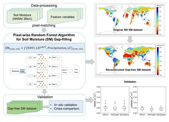
2.1. Gap-Filling Method Based on Random Forest Algorithm

The workflow of our study method is shown in Figure 1. The overall structure of this study is divided into three parts: (1) selection of feature variables that are strongly associated with surface soil moisture and can serve as independent variables for the surface soil moisture gap-filling model; (2) model training and application to establish the surface soil moisture gap-filling model by training a machine learning algorithm to identify the relationship between surface soil moisture and other independent environmental features on a pixel-by-pixel basis to generate the gap-free SM dataset at the global scale (special pixels were excluded, e.g., water, snow, ice, frozen soils or others); and (3) validation of the results by comparison with the in situ observations to illustrate the reliability of the reconstructed surface soil moisture dataset. In contrast to the traditional training model method, which inputs all samples from the whole study area into the model to obtain a training model to reconstruct the missing regions, this study uses the pixel-matching method and builds pixel-wise models for surface soil moisture gap-filling, which can improve the gap-filling accuracy and avoid the spatial discontinuity between the gap-filled values and the reference NN-SM data.

2.1.1. Principle of Random Forest

Random Forest is a highly flexible, accurate, and widely-used ensemble machine learning algorithm [38,39] that benefits from its ability to handle massive and high-dimensional datasets and to model the complex relationships between the dependent and independent variables [40]. Several specific steps are involved in the RF model. First, known values of the dependent and independent variables are input into the model as training samples. Then, a decision ‘forest’ is built by selecting different subsets of the samples to build multiple trees, and each decision tree in the forest provides a predicted value. Finally, the algorithm produces the overall average prediction value of each tree in a regression task. When splitting the tree nodes, the algorithm randomly selects a subset of features, and the optimal solution is obtained from these random combinations. As a result, the RF algorithm is not prone to overfitting and has a high tolerance for outliers and noise.

2.1.2. Selection of Feature Variables

In our study, we extracted the values of surface soil moisture data as well as the feature variables at the corresponding position pixel by pixel, and then calculated the correlation coefficient at each pixel. In addition to the dynamic variables, including Normalized Difference Vegetation Index (NDVI), land surface temperature difference between daytime and nighttime (ΔLST), and precipitation, some steady-state variables (land cover type, geographic locations) were also adopted as the independent variables for the RF-based soil moisture gap-filling model. It was confirmed that there are strong correlations between soil moisture and all the dynamic variables. These variables were selected because the surface soil moisture content is sensitive to land surface characteristics. Thus, vegetation affects surface soil moisture in different layers through the depth and extent of root distribution. Land surface temperature (LST) is mainly related to the evaporation of surface soil moisture, while precipitation can infiltrate into the soil pore space to replenish the water content of soil layers, affecting the surface soil moisture content. The validity of the selection of these feature variables has also been demonstrated by previous research results [36].

The RF algorithm can also show the relative contribution of each independent variable to the predicted variable. This contribution value is usually calculated after performing a random permutation on each feature of the data. The decrease in prediction quality can represent the importance score of the feature.

2.1.3. RF Model Establishment for SM Gap-Filling

The relationship between the SM and the selected feature variables can be expressed by:

$$S{M}_{\left(row, col\right)}=f\left(NDV{I}_{\left(row, col\right)},\Delta LS{T}_{\left(row, col\right)},P_{\left(row, col\right)},L{C}_{\left(row, col\right)}\right)$$

(1)

where $SM$ is the surface soil moisture (m³/m³), $NDVI$ is daily NDVI value, $P$ is daily total precipitation (mm), $\Delta LST$ is the daily value of daytime-nighttime LST difference (K), $LC$ is the land cover type at yearly step, and $row$ and $col$ are the row-column numbers corresponding to the latitude and longitude of each pixel.

In this study, we aim to build the pixel-wise RF model by fitting the surface soil moisture to the feature variables at each individual pixel. However, the accuracy of the model is limited by the insufficient number of data available from a single pixel due to gaps in the time series of NN-SM data. Assuming that the target pixel has similarity with the neighboring pixels in surface soil moisture and independent variables, the time series data in the 3 × 3 window of the target pixel neighborhood were taken as input to the model to increase the number of training samples.

For each pixel, all the valid data in the NN-SM time series and the corresponding independent variables are taken as the input and randomly divided into training and testing sets in a ratio of 7:3, and then the trained RF model is used to predict the absence in the time series of NN-SM. Unlike the sequential methods to separate the training and test samples, the random sample split method can randomly distribute the data between training and testing, thus ensuring the generalization ability of the model to unseen data. Each set of data contains a set of dependent variables and explanatory variables (NDVI, $\Delta LST$, P, LC). The training sets are used to build each training model, and the test sets are used to evaluate the quality of the training model. To avoid the confusion between the terms of ‘testing’ and ‘validation’, in this paper we use ‘testing’ to show the capability of the machine learning model when applied to the remaining untrained subset of the full dataset during the model development phase. We define ‘validation’ as the comparison with the in situ observations to show the accuracy of the final product, which will be described in the following sections. According to our results, the global mean of Bias was 0.0001 m³/m³ during training and 0.0003 m³/m³ during testing, which indicates that the trained model is not overfitted and is applicable to independent datasets. Finally, we reconstruct the soil moisture values in the gaps using the regression relationship constructed by the model and the feature variables.

The RF algorithm was implemented using the Regressor scikit-Learn package in Python. When splitting a node, the size of the random subset (max_features) and the number of trees (n estimators) are two key parameters that need to be determined as they affect the performance of the RF model. As recommended in the literature, after testing the model parameters [41,42], we set the parameter n_estimators as 100 and the value of max_features to none, which indicates that all features are always considered instead of a random subset.

Our computation is conducted on the big earth data cloud service platform provided by the Chinese Academy of Sciences. The adopted cloud hosting configuration includes 56 cores CPU and 160G memory, and the operating system is CentOS Linux. It takes about 5 h to complete the gap-filling for a single year at the global scale.

2.2. Evalution Metrics

First, we validated our method by creating artificial gaps in the original NN-SM dataset. We applied the trained RF model to predict SM values in these gaps, and then compared the simulated SM values with the original values that were manually removed. In addition, the reconstructed soil moisture values were quantitatively evaluated using in situ data.

Four error metrics, i.e., Bias ($Bias$, m³/m³), correlation coefficient ($R$), root mean square error ($RMSE$, m³/m³), and unbiased root mean square error ($ubRMSE$, m³/m³), were used to evaluate the results:

$$RMSE=\sqrt{\frac{{{\displaystyle \sum }}_{t=1}^N{\left(S{M}_E-S{M}_o\right)}^2}{N}}$$

(2)

$$R=\frac{Cov\left( S{M}_E-S{M}_o\right)}{{\sigma }_{S{M}_E}\ast {\sigma }_{S{M}_o}}$$

(3)

$$ubRMSE=\sqrt{\frac{ {{\displaystyle \sum }}_{i=1}^N{\left[\left(S{M}_E - E \left(S{M}_E\right)\right) - \left(S{M}_o - E \left(S{M}_o\right)\right)\right]}^2}{N}}$$

(4)

$$Bias=\frac{{{\displaystyle \sum }}_{t=1}^N\left( S{M}_E-S{M}_o\right)}{N}$$

(5)

where $S{M}_E$ (m³/m³) indicates the predicted surface soil moisture, $S{M}_o$ (m³/m³) indicates the reference or ground-truth of surface soil moisture (e.g., the in situ surface soil moisture observations), $N$ indicates the number of samples, ${\sigma }_{S{M}_E}$ (m³/m³)² and ${\sigma }_{S{M}_o}$ (m³/m³)² indicate the variance of $S{M}_E$ and $S{M}_o$, and $Cov\left( S{M}_E-S{M}_o\right)$ (m³/m³) is the covariance between the predicted and the reference surface soil moisture values.

3. Data

3.1. Surface Soil Moisture Product

The surface soil moisture dataset used in this study is called NN-SM, which is a long-term global daily dataset based mainly on AMSR-E/2 and SMAP (2002–2020) (https://doi.org/10.11888/Soil.tpdc.270960 (accessed on 1 January 2022)). The dataset was obtained from the National Tibetan Plateau/Third Pole Environment Data Center (https://data.tpdc.ac.cn, accessed on 1 January 2022). The resolution of this dataset is daily 36 km. This dataset is generated by Yao et al. [27] based on the neural network algorithm, which transfers the accuracy advantages of SMAP to AMSR-E/2. The SMAP standard surface soil moisture product, which has the advantage of good accuracy, is used as the training target, and the brightness temperatures of 6.9 GHz, 10.65 Hz, 18.7 Hz, 23.8 Hz, and 36.5 Hz of AMSR-E/2 are used as the input data to output long-term time series of surface soil moisture data. These bands are selected to generate the NN-SM product mainly because the 10.65 Hz to 23.8 GHz bands are very sensitive to surface soil moisture, while their relationship could be affected by land surface vegetation condition and emissivity, which can be reflected by the brightness temperatures in 6.9 GHz, 18.7 GHz, and 36.0 GHz bands. We used this dataset because it can reproduce the spatial and temporal distribution of SMAP SM and has a longer temporal coverage, and the accuracy is comparable to the SMAP surface soil moisture product [28].

3.2. Feature Variables Data

Table 1. The remote sensing data used in this study.

Variable Name	Data Name	Temporal Resolution	Spatial Resolution	Reference
Surface soil moisture	NN-SM	Daily	36 km	[28]
NDVI	MOD13C1	16 days	0.05°	[43]
LST	Global daily 0.05° spatiotemporal continuous land surface temperature dataset	Daily	0.05°	[44]
Precipitation	ERA5	Hourly	0.25°	[45]
Land Cover Type	MCD12C1	Yearly	0.05°	[46]

shows the list of the remote sensing data used in our study. The products of the feature variables (i.e., NDVI, LST, and precipitation) at different spatial resolutions were resampled to the same projection and 36 km spatial resolution as the NN-SM dataset using a bilinear interpolation method. The land cover data were resampled to 36 km spatial resolution using the Majority algorithm.

(a)

Normalized Difference Vegetation Index

The NDVI data used in our study is from the Moderate-resolution Imaging Spectroradiometer (MODIS) MOD13C1 product (http://reverb.echo.nasa.gov/reverb/, accessed on 1 January 2022). The spatial and the temporal resolution of the MOD13C1 NDVI data are 0.05° and 16 days, respectively. The Harmonic Analysis of Time Series (HANTS) method is used to construct the daily NDVI time series based on the 16-day MOD13C1 NDVI data following the reference [47]. The HANTS method is a time series reconstruction method based on harmonic analysis, and widely used to process satellite observed time series (e.g., NDVI) which may be contaminated by unfavorable atmospheric conditions or other factors [48]. HANTS has the advantages of decoupling the periodic vegetation phenology into harmonic components, preserving the slower phenological signals while eliminating high frequency noise induced by adverse atmospheric conditions or by instrument noise with low-pass filtering [49,50,51].

• (b) Land surface temperature

The LST dataset was downloaded from https://doi.org/10.11888/Meteoro.tpdc.271663 (accessed on 1 January 2022), which was produced by fusing the MODIS LST products and the ERA5-Land reanalysis LST based on the empirical orthogonal function interpolation method and cumulative distribution function matching method [44]. This LST dataset was used in this study because of its global spatiotemporal continuous coverage. The temporal resolution of this LST dataset is 4 times a day, with two observations in the daytime and two in the nighttime (Terra/Aqua satellites observe LST^Day/LST^Night, respectively); the spatial resolution is 0.05° and the temporal span is 2002–2020. We used data from Aqua satellite observations because it has a similar overpassing time (around 1:30 p.m.) with AMSR-E. $\Delta LST$ (K) is obtained by the following equation:

$$\Delta LST=\left|LS{T}_{Aqua}^{Day}-LS{T}_{Aqua}^{Night}\right|$$

(6)

• (c) ERA 5 Precipitation

The precipitation data are from the European Centre for Medium-Range Weather Forecasts reanalysis v5 product (ERA5) and are provided by the Copernicus Climate Change Service (C3S) Climate Date Store (https://cds.climate.copernicus.eu/, accessed on 1 January 2022). The ERA5 precipitation data have an original spatial resolution of 0.25° and a temporal resolution of 1 h, with accumulation to daily totals.

• (d) Land Cover Type

The land cover type data are from the MODIS global land cover product MCD12C1 (https://lpdaac.usgs.gov/products/mcd12c1v006, accessed on 1 July 2022), with a spatial resolution of 0.05° and a temporal resolution of 1 year [45]. This study used the International Geosphere Biosphere Programme (IGBP) global vegetation classification scheme from MCD12C1, which contains 17 major land cover types.

3.3. In Situ Observations Data

We used in situ soil moisture observations as reference to verify the gap-filled SM results. The in situ surface soil moisture data from 12 measurement sites (Figure 2,

Table 2. List of validation sites.

Networks	Sites Names	Stations	Climate Regime	IGBP Land Cover	Measured Depth	Reference
Tibetan Plateau (Asia)	Pali	24	Arid	Barren/sparse	5 cm	[55]
	Naqu	57	Polar	Grasslands
OZNET (Australia)	Yanco	12	Semi-arid	Croplands/Grasslands	5–8 cm	[56]
	Kyeamba	8	Temperate	Croplands
REMEDHUS (Europe)	REMEDHUS	23	Temperate	Croplands	5 cm	[57]
AMMA (Africa)	Benin	4	Arid	Savannas	5 cm	[58,59,60,61]
	Niger	3	Arid	Grasslands
USDA (North America)	Little River	33	Temperate	Croplands	5 cm	[62,63,64,65,66]
	Little Washita	20	Temperate	Grasslands
	Walnut Gulch	19	Arid	Shrub open rangeland
	Fort Cobb	15	Temperate	Croplands
	Reynolds Creek	20	Arid	Grasslands

) are provided by the ISMN website (https://ismn.earth/en/, accessed on 1 July 2022) [52,53,54] and the Long-Term Agroecosystem Research (LTAR) network (https://ltar.ars.usda.gov/, accessed on 1 July 2022).

4. Results

4.1. RF Training Results

4.1.1. Importance of Feature Variables in RF Model Construction

Figure 3 shows the spatial distribution of the most important feature variables in the RF construction at each pixel. Daily values of NDVI, $\Delta LST$ and precipitation are important factors in most parts of the world, which was confirmed by the sensitivity and correlation between soil moisture and input variables [67]. In general, daily precipitation and surface soil moisture were positively correlated, and high surface soil moisture values were accompanied by high precipitation. In tropical rainforest areas (such as the Amazon basin and the Congo basin) with higher vegetation density, NDVI contributes the most to the predicted surface soil moisture in the RF gap-filling model, similar to the results found the previous study [68]. In the dry land regions (usually with long sunshine hours and large diurnal temperature ranges) such as the Sahara Desert, Central Asia and West Asia, the day-night land surface temperature difference is related to the soil moisture status, partly because wet (dry) soil generally results in high (low) evapotranspiration and further causes the decrease (increase) of daytime land surface temperature. Meanwhile, the response of NDVI to surface soil moisture change has a relatively long time lag, which may also reduce the importance of NDVI in explaining the soil moisture change in the dry land areas. Furthermore, the uncertainty of the precipitation data (generally very low amount of precipitation in these regions) may be related to the relative low importance of the precipitation. These factors lead to $\Delta LST$ being an important feature of the model to explain the dynamic variations of soil moisture in these dry land regions.

4.1.2. Evaluation of Model Performance

Figure 4 shows the global distribution of R and RMSE between the RF model predicted surface soil moisture and the reference (NN-SM) values for the test samples. The surface soil moisture values predicted by the RF model showed a strong correlation with the NN-SM values for most of the test samples around the world. The global average value of R is 0.68, indicating a moderate-to-strong correlation between the predicted and reference values of surface soil moisture on a global scale. Notably, higher correlation coefficients were obtained for several regions, including southern Asia, southern and central Africa, and northern North America. Additionally, particularly high correlation coefficients were observed in Australia, where vegetation cover was low to moderate. Regions with high vegetation cover, such as the Amazon and Congo rainforests, were found to have lower R than other regions. This result was expected, because dense vegetation cover and persistently high levels of surface soil moisture can make accurate predictions of surface soil moisture difficult. The overall RMSE at the global scale is 0.044 m³/m³ (Figure 4b). Our analysis revealed those areas with sparse vegetation or bare soil, such as arid, semi-arid, and desert regions, had low values of RMSE, as expected, since low soil moisture values and a narrow range are predominant in these regions. For example, locations such as Australia, the Sahara, and southern North America had low RMSE values. The areas with medium to high vegetation or covered by alpine flora, such as southern Asia, India, and southeastern Australia, were found to have higher RMSE values. One possible reason is that the C-and X-bands are sensitive to the presence of vegetation, and the amount and density of vegetation cover can significantly affect the accuracy of surface soil moisture obtained by AMSR-E/2. This suggests that the model based on AMSR-E/2 observations may be less effective in accurately predicting surface soil moisture levels in these types of environments, particularly in areas near the Earth’s equator. The L-band sensor on board SMAP is less affected by vegetation and therefore may have better accuracy in the densely vegetated regions. The R values of the test samples are mostly medium to high, indicating a significant correlation between the predicted and observed surface soil moisture values. In addition, the RMSE values are moderate but within a range that is acceptable and reasonable. The results presented above demonstrate that the trained random forest models performed well and could be used to reconstruct the missing values of the NN-SM.

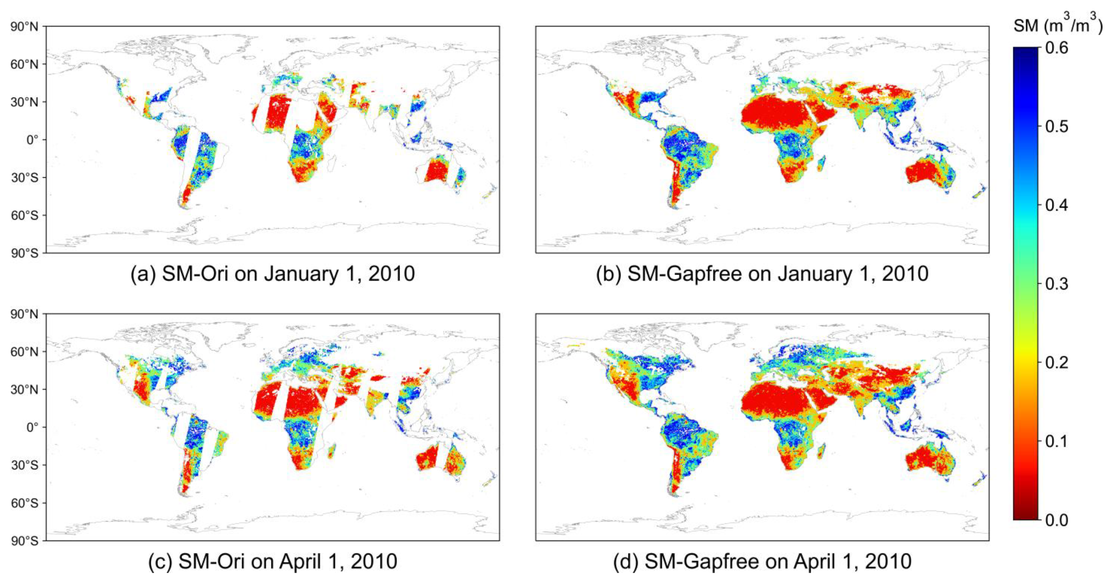
4.2. Reconstruction Results and Cross-Comparison

Figure 5 shows the spatial distributions of the fractional valid observations (valid surface soil moisture values recorded in the dataset) of the original NN-SM (SM-Ori) and gap-free dataset after reconstruction (SM-Gapfree). As expected, fewer observations are available in the high-altitude areas, such as the Tibetan Plateau, and in high-latitude regions in the northern hemisphere in the original NN-SM. The global average coverage of the NN-SM product is 53.2% (excluding Antarctica and Greenland), while the global coverage ratio of our gap-free SSM dataset has increased significantly (up to 85%). The global coverage ratio of our gap-free SSM dataset can even reach 100% for areas without snow/ice, frozen soil or water coverage. For the high-altitude areas and high-latitude regions, the reconstruction method is influenced by the special pixels, e.g., water, snow/ice, frozen soils pixels.

The coverage ratio also shows a temporal variation. Figure 6 shows the global averaged land coverage ratio of the original NN-SM data and our gap-free SM data at daily step in 2015. The daily fraction of valid data in the original NN-SM data ranges from 21.4% to 74.55%, with low values from December to the following February (winter in the Northern Hemisphere) and high values from June to August (summer in the Northern Hemisphere). The gaps could be significantly reduced and gap-free soil moisture data could be obtained temporally by our method. This gap-free database is important for comprehensive analysis and research.

The reconstructed surface soil moisture dataset from 2002 to 2020 was produced by applying the gap-filling algorithm developed in Section 2 to the original NN-SM product. Figure 7 shows the results of the original and reconstructed global daily surface soil moisture on 1 January, 1 April, 1 July, and 1 October in 2010. The left column of Figure 7 lists the original NN-SM with gaps (referred to as SM-Ori), and the right column presents the SM after gap-filling using the proposed method (SM-Gapfree). The original NN-SM product does not cover Antarctica and Greenland due to the persistent snow and ice cover, so we have not included these regions in the reconstructed SM dataset. The resulting gap-free dataset shows significant improvements in representing the continuity and variability of surface soil moisture at a global scale and demonstrates the effectiveness of a pixel-wise training approach in the RF algorithm.

Moreover, we compared the reconstructed results obtained using our pixel-wise RF with the results from the RF trained in a traditional global uniform (TGU) manner gap-filling method; the TGU gap-filling method takes all samples in the model to build a training model that uniformly fills the global missing data. The global uniform gap filling method has been widely used in previous studies [41]. Here, we implement the global uniform gap filling method following the procedure of Sun and Hao [41] for comparison with our pixel-wise method. The comparisons of reconstructed surface soil moisture produced by the traditional training model and the pixel-wise machine learning model proposed in this study are shown in Figure 8. As shown in Figure 8(c1–c4), we can see obvious spatial discontinuity in the reconstructed results obtained by traditional training methods. In contrast, the pixel-wise method proposed in this study performs better in terms of spatial continuity, and no obvious boundary could be found around the filled regions in Figure 8(d1–d4). This indicates that the gap-filling approach in our study is superior to the traditional method.

In addition to evaluating the reconstruction results in gaps, we also evaluated the results of the RF model by creating artificial gaps in the NN-SM dataset and then compared the surface soil moisture values predicted by the RF model with the original values of the NN-SM dataset that had been removed. We carried out such a cross-comparison in five sub-regions across different continents on typical winter and summer days, 1 January 2019 and 1 July 2019, respectively, as shown in Figure 9. Overall, the simulated surface soil moisture results have a high consistency with the original products as demonstrated in these sub-regions (Figure 9), indicating that the RF model can reproduce the values of the original NN-SM dataset. Differences could be found in some areas in Figure 9(c1,d1,h1,i1), where the simulated surface soil moisture values slightly overestimated or underestimated the corresponding original values, probably impacted by the land use and land cover type. The overestimation occurred primarily in short vegetation areas such as croplands and grasslands, while the underestimation occurred primarily in woody areas. Forest generally has a higher vegetation optical depth than croplands and grasslands; this may introduce larger uncertainty in the soil moisture retrieved from microwave brightness temperature observations for forest regions, which could partly explain the difference. We also observed significant seasonal variations in surface soil moisture in croplands and grasslands. During the peak growing season, the vegetation optical depth is higher than that during the early and end stages of the growing seasons, and it can also affect the accuracy of the NN-SM soil moisture and our gap-filling results.

We created scatterplots to further demonstrate quantitatively the agreement between simulated surface soil moisture and the original NN-SM data over the five sub-regions on 1 January and 1 July in randomly selected years of 2003, 2008, 2014 and 2019 (Figure 10 and Figure 11). The simulated surface soil moisture showed high agreement with the original NN-SM data, with R values ranging from 0.768 to 0.919, RMSE values from 0.053 to 0.082 m³/m³, ubRMSE values from 0.053 to 0.081 m³/m³, and bias values from −0.007 to 0.010 m³/m³, respectively.

Figure 12 shows the boxplots of the evaluation metrics (R, RMSE, ubRMSE and Bias), and it clearly shows the good accuracy of our pixel-wise RF method. Figure 13 shows the histogram distribution of the reconstructed surface soil moisture values in the typical simulated sub-regions by different methods on 1 January and 1 July 2019, respectively. Regardless of high or low surface soil moisture values, our method generally produced results consistent with the distribution of the original data. The distribution of the results by the global uniform method shows large bias in terms of peak and frequency, when compared with the original data.

4.3. Validation Using the In Situ Observations

The reconstructed surface soil moisture values were validated using the in situ observations at the selected 12 validation sites. For a better comparison, we present the statistical metrics between the datasets of the original SM (SM-Ori), the gap-filled SM (referred to as SM-Recon), the result of merging the original SM and the gap-filled SM (referred to as SM-Gapfree), respectively, with the in situ observations in

Table 3. Statistical comparisons of the SM-Ori, SM-Recon, and SM-Gapfree with the in situ SM.

	R			RMSE (m3/m3)			ubRMSE (m3/m3)			Bias (m3/m3)
Sites	SM -Ori	SM -Recon	SM -Gapfree	SM -Ori	SM -Recon	SM -Gapfree	SM -Ori	SM -Recon	SM -Gapfree	SM -Ori	SM -Recon	SM -Gapfree
Benin	0.800	0.853	0.818	0.120	0.112	0.117	0.058	0.042	0.052	0.105	0.104	0.104
Fort Cobb	0.495	0.447	0.453	0.061	0.049	0.061	0.061	0.048	0.061	−0.004	−0.006	−0.002
Kyemba	0.740	0.613	0.708	0.105	0.108	0.105	0.079	0.074	0.076	0.070	0.079	0.073
Little River	0.539	0.552	0.505	0.138	0.126	0.137	0.054	0.037	0.051	0.127	0.121	0.127
Little Washita	0.498	0.391	0.452	0.066	0.052	0.065	0.062	0.051	0.061	0.024	0.011	0.023
Naqu	0.810	0.751	0.809	0.075	0.072	0.074	0.071	0.054	0.053	−0.025	−0.049	−0.052
Niger	0.786	0.669	0.708	0.033	0.044	0.038	0.025	0.023	0.026	0.021	0.037	0.029
Pali	0.598	0.811	0.811	0.051	0.03	0.038	0.028	0.029	0.032	−0.043	−0.009	−0.02
Remedhus	0.835	0.76	0.826	0.036	0.034	0.034	0.036	0.034	0.034	−0.001	0.002	−0.001
Reynolds Creek	0.497	0.423	0.468	0.069	0.057	0.07	0.067	0.057	0.067	0.016	0.003	0.018
Walnut Gulch	0.574	0.553	0.572	0.065	0.051	0.058	0.044	0.028	0.036	0.047	0.043	0.046
Yanco	0.770	0.628	0.737	0.080	0.072	0.076	0.062	0.062	0.061	0.050	0.036	0.045
all	0.662	0.621	0.656	0.075	0.067	0.073	0.054	0.045	0.051	0.032	0.031	0.033

and Figure 14. For the results of SM-Ori, SM-Recon, and SM-Gapfree, the range of R was between 0.391 and 0.853, the ubRMSE values were between 0.023 m³/m³ and 0.074 m³/m³, and the Bias values were between −0.049 m³/m³ and 0.104 m³/m³. Some low R values were found, mainly due to large differences between the original SM data and the observations at the in situ sites. The mean R, RMSE, ubRMSE, and Bias of the reconstructed gap-free SM (original) data were 0.656 (0.662), 0.073 m³/m³ (0.075 m³/m³), 0.051 m³/m³ (0.054 m³/m³), and 0.033 m³/m³ (0.032 m³/m³), respectively. Overall, the accuracy of the reconstructed surface soil moisture products was high, and the reconstructed surface soil moisture product maintained the same level of accuracy as the original NN-SM product (Table 3 and Figure 14), which verified the reliability and usability of the generated spatiotemporal continuous SM products.

Figure 15 shows the time series of the reconstructed (SM-Recon) and the in situ observations at 6 selected validation sites (each from one continent) from 2010 to 2016 to further validate the performance of the reconstructed products. The variation of in situ surface soil moisture ranged from 0.1 to 0.6 m³/m³ with different magnitudes at different sites, and the reconstructed surface soil moisture data could reproduce similar daily dynamics to the observations. The reconstructed surface soil moisture showed inter-annual variability and correlated with the temporal pattern of precipitation at most sites. Low values of surface soil moisture occurred mainly in the dry seasons and winter frozen periods, and high values of surface soil moisture occurred mainly during the wet and rainy summer seasons. In general, the reconstructed surface soil moisture data could not only maintain temporal consistency with the in situ surface soil moisture data, but also reflected the dynamic variability of surface soil moisture. The reliability of the proposed method and the usability of the established gap-free surface soil moisture product were demonstrated by the time series validation, which is of great practical significance for the application and analysis of long-time series products.

Figure 16 shows the scatterplots of the reconstructed surface soil moisture (also the original values) against the in situ observations. The reconstructed surface soil moisture values at different sites were not significantly different from the site observations, indicating a good agreement with the in situ surface soil moisture values. For example, the comparison at the Benin site in Africa showed that the R for the original product was 0.800 (ubRMSE was 0.058 m³/m³), while the R for the reconstructed data was 0.853 (ubRMSE was 0.042 m³/m³); for the Little River site in the United States, the correlation for the original surface soil moisture product was 0.539 (ubRMSE was 0.054 m³/m³), while the correlation of the reconstructed results changed to 0.553 (ubRMSE was 0.037 m³/m³). This was a satisfactory validation of the research method, since our goal was to extend the established original surface soil moisture products to the areas where data were missing, rather than to improve the accuracy of the retrieval algorithm itself. The R values are high, ranging from 0.553 to 0.853. The lower RMSE values are 0.034 m³/m³ at the REMEDHUS sites and 0.044 m³/m³ at the Niger sites, where the dynamic range of surface soil moisture is small. The lower R values at the Little River sites compared to the original surface soil moisture may be due to errors in the original product. In addition, the reconstructed results have lower Bias values, indicating that the reconstructed product has good consistency and stability.

5. Discussion

5.1. The Proposed Pixel-Wise RF Method and the Gap-Filling Results

Applications of surface soil moisture products based on satellite remote sensing observations are often hampered by gaps in the time series. The spatiotemporal gaps in the satellite remotely sensed surface soil moisture data are caused by a variety of factors, such as different satellite revisit times, human-induced radio frequency interference contamination, presence of ice, snow or frozen ground, and high uncertainty of retrievals in coastal and mountain areas; some of these problems cannot be mitigated by increasing the number of sensors or improving the data fusion techniques [69,70,71,72,73]. The successful applications of machine learning based gap-filling methods at regional scale are based on the fact that SM is somehow related to other variables, e.g., precipitation, NDVI, LST, terrain. In this study, we reconstructed the data to fill the gaps in the NN-SM product using the RF algorithm in a pixel-wise manner, which performed much better than the global uniform RF model for surface soil moisture gap-filling, as shown in the results section. The global gap-free dataset with spatiotemporal continuity (SM-Gapfree) could be obtained by merging our gap-filled values with the original NN-SM dataset. The accuracy of the gap-filling and the obtained gap-free dataset were well illustrated by comparison with the ground observations.

We also realize that the physical basis of our gap-filling method for the pixels covered by snow/ice or frozen soil need further investigation. Although it may be controversial, some datasets retain the surface soil moisture values for these special pixels (water, snow, ice, frozen soil or others); for example, the ERA5 global reanalysis data also gives the soil moisture value for the water and snow/ice covered pixels. It is also noteworthy that even though the amount of liquid water in the frozen soil is very small, it is not negligible. For example, a recent study shows that the soils in permafrost regions of Alaska contain 5–25% liquid water at near freezing temperatures; this plays a very important role, particularly in promoting permafrost thaw, controlling cold-season carbon emissions, and enhancing the microbial carbon release prior to permafrost collapse [74]. Similar results were also found in high altitude areas in the Tibetan Plateau, such as Naqu and Maqu, where both surface and root zone soil moisture values based on in situ observations were above zero even during the cold winter [55,75]. To avoid the controversy, in this study, we used a method to exclude (flag) the pixels covered by frozen soil, snow/ice and water. The water and permanent snow/ice covered pixels were first masked based on the annual MODIS land cover product; further, pixels with daytime land surface temperature lower than 0 °C were labeled and excluded in our daily soil moisture dataset. We constructed a flag layer to easily distinguish different data quality levels of our gap-free dataset: “0” represents the original surface soil moisture value from NN-SM; “1” represents the gap-filled surface soil moisture value; “2” represents the excluded pixels relating to areas that are covered by water or snow/ice, and frozen soils. A similar strategy to exclude the special pixels is also commonly adopted in other microwave remote sensing soil moisture product, e.g., the ESA-CCI soil moisture product, which provides a flag of ‘Snow_coverage_or_temperature_below_zero’ based on land surface temperature [76]. Further studies will be conducted to explore the rationale for and possibility of obtaining soil moisture values in frozen soil to further improve our understanding.

5.2. Uncertainty Analysis of the Gap-Free Results

Most satellite-based surface soil moisture products have data gaps. The NN-SM data product can reproduce the spatial and temporal distribution of SMAP SM with a longer time series, and the accuracy is comparable to that of the SMAP surface soil moisture product. However, there are inevitable gaps in the NN-SM product, mainly caused by various factors such as satellite revisit times, human-induced radio frequency interference, presence of ice, snow or frozen ground, and errors of soil moisture retrievals in coastal and mountain regions.

A variety of machine learning techniques have been evaluated and applied to fill gaps in surface soil moisture data [35,36,37]. The successful regional applications of machine learning-based gap-filling methods are built on the assumptions that surface soil moisture is somehow related to other variables, such as precipitation, NDVI, LST, etc. However, when the model is established by training the machine learning in a traditional way, it cannot fully fit all the details and often results in a boundary effect between the filled and the original values (a phenomenon where the reconstruction results do not quite match the spatial characteristics of the original NN-SM product in some areas, as shown in Figure 8). This study proposed to build a pixel-wise machine learning model by training the model with the sample data developed in each pixel, and it performed much better in terms of spatial continuity and accuracy. The quantitative validation based on in situ observations also shows the validity of the gap-filling method and the good accuracy of the generated gap-free surface soil moisture dataset.

The uncertainty in the original NN-SM dataset should be mentioned because the gap-free SM in this study is obtained by filling the gaps in the NN-SM dataset. The errors in the original surface soil moisture product, as shown in Figure 11, will inevitably be transferred to the reconstructed product. The external uncertainties in the selected input datasets as feature variables will certainly be propagated into the gap-free SM dataset. In addition to the uncertainties of the NDVI and LST data (mainly based on MODIS) themselves, the use of the satellite-based instantaneous information as a surrogate to characterize the all-weather surface state will also introduce uncertainties [77,78]. In addition, the relationship between surface soil moisture and precipitation is complicated, including some mismatch between the adopted ERA5 precipitation and NN-SM dataset which could be seen during the study; this certainly affects the accuracy of the reconstructed surface soil moisture. Precipitation is one of the most important factors affecting surface soil moisture, as it is the main source of soil moisture. The inherent errors in the precipitation data can affect the prediction of surface soil moisture when propagated through reconstruction models [79].

In addition, the setting of parameters is very important for the training accuracy of the machine learning method. The purpose of adjusting the parameters is to achieve the maximum harmony of the deviation and variance in the model. The models of this study are established pixel-by-pixel; considering the computation time, we did not search for the optimal parameter at each pixel. This uncertainty may affect the parameter generalization of the proposed gap-filling model to some extent. In addition, the spatial component was not considered during the samples separation. Since our model is based on a pixel-by-pixel basis, the model itself is constructed within each pixel and its neighborhood pixels. We also notice that the RF algorithm can lead to more centralized values in the predicted results. This could happen because RF tends to fit to the mean of the dependent variable while ignoring the extremes. It may overestimate the likelihood of average outcomes and underestimate the probability of extreme outcomes. This problem is especially severe for the global uniform method. The pixel-wise RF method proposed in this study significantly improves the accuracy under the extreme conditions, but some bias still exists. Further improvement on the RF algorithm may be helpful to solve this problem.

6. Conclusions

In this paper, a pixel-wise machine learning (Random Forest) model was developed to fill the gaps in the NN-SM product and the reconstructed gap-free of surface soil moisture product was generated from 2002 to 2020. Various feature variables were used to build the pixel-wise RF model, such as NDVI, precipitation, LST, land cover type. The model training and validation, as well as the application, were conducted in a pixel-by-pixel manner to account for the difference between different geographical locations, which proved to be helpful improving the gap-filling accuracy and spatial discontinuity of the dataset. The evaluation was conducted by comparing the reconstructed SM with the in situ surface soil moisture observations and by cross-comparison with the original surface soil moisture product.

The main conclusions of this study are as follows: (1) The NN-SM dataset frequently exhibits gaps on a global scale. These gaps are not restricted to specific geographical regions or seasons, as they are observed in both warm and cold periods and regions. The largest fraction of non-valid data is more than 80%, and the average gap percentage is about 53% globally. (2) The pixel-wise RF method developed in this study has a stronger gap-filling ability after careful quality evaluation, which achieved a good agreement with the NN-SM, with R of 0.649 and RMSE of 0.050 m³/m³ globally. These well-validated indicators ensure the reliability of the long-term dataset of surface soil moisture that will be produced by subsequent steps. (3) The pixel-wise RF model performed well based on the comparison with the original NN SM product as demonstrated over the ten simulated areas with R ranging from 0.770 to 0.918, ubRMSE from 0.053 to 0.081 m³/m³, and Bias from −0.012 to 0.008 m³/m³. Compared to the in situ surface soil moisture observations of the ISMN networks, the pixel-wise RF model achieved good performance with R of 0.610, ubRMSE of 0.045 m³/m³ and Bias of 0.031 m³/m³. The evaluation results highlighted the high accuracy and reliability of the generated global long-term gap-free surface soil moisture dataset. In conclusion, our research demonstrates that a pixel-wise training approach for the Random Forest machine learning can effectively reconstruct global gap-free surface soil moisture products. The approach we have developed holds promise for future application to soil moisture products from other satellite missions, provided that sufficient time series samples are available.

References

1. Gianotti, D.J.S.; Akbar, R.; Feldman, A.F.; Salvucci, G.D.; Enthekabi, D. Terrestrial Evaporation and Moisture Drainage in a Warmer Climate. Geophys. Res. Lett. 2020, 47, e2019GL086498. [Google Scholar] [CrossRef]
2. Oki, T.; Kanae, S.; Musiake, K. Global hydrological cycle and world water resources. Membrane 2003, 28, 206–214. [Google Scholar] [CrossRef]
3. Liu, Y.; Zhu, Y.; Zhang, L.Q.; Ren, L.L.; Yuan, F.; Yang, X.L.; Jiang, S.H. Flash droughts characterization over China: From a perspective of the rapid intensification rate. Sci. Total Environ. 2020, 704, 135373. [Google Scholar] [CrossRef] [PubMed]
4. Wei, L.Y.; Jiang, S.H.; Ren, L.L.; Yuan, F.; Zhang, L.Q. Performance of Two Long-Term Satellite-Based and GPCC 8.0 Precipitation Products for Drought Monitoring over the Yellow River Basin in China. Sustainability 2019, 11, 4969. [Google Scholar] [CrossRef]
5. Zhang, L.Q.; Liu, Y.; Ren, L.L.; Jiang, S.H.; Yang, X.L.; Yuan, F.; Wang, M.H.; Wei, L.Y. Drought Monitoring and Evaluation by ESA CCI Soil Moisture Products Over the Yellow River Basin. IEEE J. Sel. Top. Appl. Earth Obs. Remote Sens. 2019, 12, 3376–3386. [Google Scholar] [CrossRef]
6. Teuling, A.J. CLIMATE HYDROLOGY A hot future for European droughts. Nat. Clim. Chang. 2018, 8, 364–365. [Google Scholar] [CrossRef]
7. Laiolo, P.; Gabellani, S.; Campo, L.; Silvestro, F.; Delogu, F.; Rudari, R.; Pulvirenti, L.; Boni, G.; Fascetti, F.; Pierdicca, N.; et al. Impact of different satellite soil moisture products on the predictions of a continuous distributed hydrological model. Int. J. Appl. Earth Obs. Geoinf. 2016, 48, 131–145. [Google Scholar] [CrossRef]
8. Collow, T.W.; Robock, A.; Wu, W. Influences of soil moisture and vegetation on convective precipitation forecasts over the United States Great Plains. J. Geophys. Res. Atmos. 2014, 119, 9338–9358. [Google Scholar] [CrossRef]
9. Dirmeyer, P.A.; Guo, Z.C.; Gao, X. Comparison, validation, and transferability of eight multiyear global soil wetness products. J. Hydrometeorol. 2004, 5, 1011–1033. [Google Scholar] [CrossRef]
10. Njoku, E.G.; Jackson, T.J.; Lakshmi, V.; Chan, T.K.; Nghiem, S.V. Soil moisture retrieval from AMSR-E. IEEE Trans. Geosci. Remote Sens. 2003, 41, 215–229. [Google Scholar] [CrossRef]
11. Robock, A.; Vinnikov, K.Y.; Srinivasan, G.; Entin, J.K.; Hollinger, S.E.; Speranskaya, N.A.; Liu, S.X.; Namkhai, A. The Global Soil Moisture Data Bank. Bull. Am. Meteorol. Soc. 2000, 81, 1281–1299. [Google Scholar] [CrossRef]
12. Al-Yaari, A.; Wigneron, J.P.; Ducharne, A.; Kerr, Y.; de Rosnay, P.; de Jeu, R.; Govind, A.; Al Bitar, A.; Albergel, C.; Munoz-Sabater, J.; et al. Global-scale evaluation of two satellite-based passive microwave soil moisture datasets (SMOS and AMSR-E) with respect to Land Data Assimilation System estimates. Remote Sens. Environ. 2014, 149, 181–195. [Google Scholar] [CrossRef]
13. Raoult, N.; Delorme, B.; Ottle, C.; Peylin, P.; Bastrikov, V.; Maugis, P.; Polcher, J. Confronting Soil Moisture Dynamics from the ORCHIDEE Land Surface Model with the ESA-CCI Product: Perspectives for Data Assimilation. Remote Sens. 2018, 10, 1786. [Google Scholar] [CrossRef]
14. Loew, A.; Ludwig, R.; Mauser, W. Derivation of surface soil moisture from ENVISAT ASAR wide swath and image mode data in agricultural areas. IEEE Trans. Geosci. Remote Sens. 2006, 44, 889–899. [Google Scholar] [CrossRef]
15. Zeng, J.Y.; Li, Z.; Chen, Q.; Bi, H.Y.; Qiu, J.X.; Zou, P.F. Evaluation of remotely sensed and reanalysis soil moisture products over the Tibetan Plateau using in-situ observations. Remote Sens. Environ. 2015, 163, 91–110. [Google Scholar] [CrossRef]
16. Du, J.Y.; Kimball, J.S.; Jones, L.A.; Kim, Y.; Glassy, J.; Watts, J.D. A global satellite environmental data record derived from AMSR-E and AMSR2 microwave Earth observations. Earth Syst. Sci. Data 2017, 9, 791–808. [Google Scholar] [CrossRef]
17. Du, J.Y.; Kimball, J.S.; Shi, J.C.; Jones, L.A.; Wu, S.L.; Sun, R.J.; Yang, H. Inter-Calibration of Satellite Passive Microwave Land Observations from AMSR-E and AMSR2 Using Overlapping FY3B-MWRI Sensor Measurements. Remote Sens. 2014, 6, 8594–8616. [Google Scholar] [CrossRef]
18. Feng, X.M.; Li, J.X.; Cheng, W.; Fu, B.J.; Wang, Y.Q.; Lu, Y.H.; Shao, M.A. Evaluation of AMSR-E retrieval by detecting soil moisture decrease following massive dryland re-vegetation in the Loess Plateau, China. Remote Sens. Environ. 2017, 196, 253–264. [Google Scholar] [CrossRef]
19. Kim, H.; Parinussa, R.; Konings, A.G.; Wagner, W.; Cosh, M.H.; Lakshmi, V.; Zohaib, M.; Choi, M. Global-scale assessment and combination of SMAP with ASCAT (active) and AMSR2 (passive) soil moisture products. Remote Sens. Environ. 2018, 204, 260–275. [Google Scholar] [CrossRef]
20. Kim, S.; Liu, Y.Y.; Johnson, F.M.; Parinussa, R.M.; Sharma, A. A global comparison of alternate AMSR2 soil moisture products: Why do they differ? Remote Sens. Environ. 2015, 161, 43–62. [Google Scholar] [CrossRef]
21. Tuttle, S.E.; Salvucci, G.D. A new approach for validating satellite estimates of soil moisture using large-scale precipitation: Comparing AMSR-E products. Remote Sens. Environ. 2014, 142, 207–222. [Google Scholar] [CrossRef]
22. van der Velde, R.; Su, Z.B.; van Oevelen, P.; Wen, J.; Ma, Y.M.; Salama, M.S. Soil moisture mapping over the central part of the Tibetan Plateau using a series of ASAR WS images. Remote Sens. Environ. 2012, 120, 175–187. [Google Scholar] [CrossRef]
23. Yang, H.; Weng, F.Z.; Lv, L.Q.; Lu, N.M.; Liu, G.F.; Bai, M.; Qian, Q.Y.; He, J.K.; Xu, H.X. The FengYun-3 Microwave Radiation Imager On-Orbit Verification. IEEE Trans. Geosci. Remote Sens. 2011, 49, 4552–4560. [Google Scholar] [CrossRef]
24. Chan, S.K.; Bindlish, R.; O’Neill, P.E.; Njoku, E.; Jackson, T.; Colliander, A.; Chen, F.; Burgin, M.; Dunbar, S.; Piepmeier, J.; et al. Assessment of the SMAP Passive Soil Moisture Product. IEEE Trans. Geosci. Remote Sens. 2016, 54, 4994–5007. [Google Scholar] [CrossRef]
25. Colliander, A.; Jackson, T.J.; Bindlish, R.; Chan, S.; Das, N.; Kim, S.B.; Cosh, M.H.; Dunbar, R.S.; Dang, L.; Pashaian, L.; et al. Validation of SMAP surface soil moisture products with core validation sites. Remote Sens. Environ. 2017, 191, 215–231. [Google Scholar] [CrossRef]
26. Xie, Q.; Jia, L.; Menenti, M.; Hu, G. Global soil moisture data fusion by Triple Collocation Analysis from 2011 to 2018. Sci. Data 2022, 9, 687. [Google Scholar] [CrossRef] [PubMed]
27. Yao, P.; Shi, J.; Zhao, T.; Lu, H.; Al-Yaari, A. Rebuilding long time series global soil moisture products using the neural network adopting the microwave vegetation index. Remote Sens. 2017, 9, 35. [Google Scholar] [CrossRef]
28. Yao, P.; Lu, H.; Shi, J.; Zhao, T.; Yang, K.; Cosh, M.H.; Gianotti, D.J.S.; Entekhabi, D. A long term global daily soil moisture dataset derived from AMSR-E and AMSR2 (2002–2019). Sci. Data 2021, 8, 143. [Google Scholar] [CrossRef]
29. Cho, E.S.; Su, C.H.; Ryu, D.; Kim, H.; Choi, M. Does AMSR2 produce better soil moisture retrievals than AMSR-E over Australia? Remote Sens. Environ. 2017, 188, 95–105. [Google Scholar] [CrossRef]
30. Long, D.; Bai, L.L.; Yan, L.; Zhang, C.J.; Yang, W.T.; Lei, H.M.; Quan, J.L.; Meng, X.Y.; Shi, C.X. Generation of spatially complete and daily continuous surface soil moisture of high spatial resolution. Remote Sens. Environ. 2019, 233, 111364. [Google Scholar] [CrossRef]
31. Guo, G.; Zhao, B. Monitoring soil moisture content with modis data. Soil 2004, 36, 219–221. [Google Scholar]
32. Llamas, R.M.; Guevara, M.; Rorabaugh, D.; Taufer, M.; Vargas, R. Spatial Gap-Filling of ESA CCI Satellite-Derived Soil Moisture Based on Geostatistical Techniques and Multiple Regression. Remote Sens. 2020, 12, 665. [Google Scholar] [CrossRef]
33. Sandholt, I.; Rasmussen, K.; Andersen, J. A simple interpretation of the surface temperature/vegetation index space for assessment of surface moisture status. Remote Sens. Environ. 2002, 79, 213–224. [Google Scholar] [CrossRef]
34. Wang, G.J.; Garcia, D.; Liu, Y.; de Jeu, R.; Dolman, A.J. A three-dimensional gap filling method for large geophysical datasets: Application to global satellite soil moisture observations. Environ. Model. Softw. 2012, 30, 139–142. [Google Scholar] [CrossRef]
35. Ahmad, S.; Kalra, A.; Stephen, H. Estimating soil moisture using remote sensing data: A machine learning approach. Adv. Water Resour. 2010, 33, 69–80. [Google Scholar] [CrossRef]
36. Liu, Y.X.Y.; Yang, Y.P.; Jing, W.L.; Yue, X.F. Comparison of Different Machine Learning Approaches for Monthly Satellite-Based Soil Moisture Downscaling over Northeast China. Remote Sens. 2018, 10, 31. [Google Scholar] [CrossRef]
37. Zhang, Q.; Yuan, Q.Q.; Li, J.; Wang, Y.; Sun, F.J.; Zhang, L.P. Generating seamless global daily AMSR2 soil moisture (SGD-SM) long-term products for the years 2013–2019. Earth Syst. Sci. Data 2021, 13, 1385–1401. [Google Scholar] [CrossRef]
38. Chan, J.C.-W.; Paelinckx, D. Evaluation of Random Forest and Adaboost tree-based ensemble classification and spectral band selection for ecotope mapping using airborne hyperspectral imagery. Remote Sens. Environ. 2008, 112, 2999–3011. [Google Scholar] [CrossRef]
39. Rodriguez-Galiano, V.F.; Ghimire, B.; Rogan, J.; Chica-Olmo, M.; Rigol-Sanchez, J.P. An assessment of the effectiveness of a random forest classifier for land-cover classification. ISPRS J. Photogramm. Remote Sens. 2012, 67, 93–104. [Google Scholar] [CrossRef]
40. Hutengs, C.; Vohland, M. Downscaling land surface temperatures at regional scales with random forest regression. Remote Sens. Environ. 2016, 178, 127–141. [Google Scholar] [CrossRef]
41. Sun, H.; Xu, Q. Evaluating Machine Learning and Geostatistical Methods for Spatial Gap-Filling of Monthly ESA CCI Soil Moisture in China. Remote Sens. 2021, 13, 2848. [Google Scholar] [CrossRef]
42. Rahmati, O.; Falah, F.; Dayal, K.S.; Deo, R.C.; Mohammadi, F.; Biggs, T.; Moghaddam, D.D.; Naghibi, S.A.; Bui, D.T. Machine learning approaches for spatial modeling of agricultural droughts in the south-east region of Queensland Australia. Sci. Total Environ. 2020, 699, 134230. [Google Scholar] [CrossRef]
43. Didan, K. MOD13C1 MODIS/Terra Vegetation Indices 16-Day L3 Global 0.05Deg CMG V006. Distributed by NASA EOSDIS Land Processes DAAC. 2015. Available online: https://doi.org/10.5067/MODIS/MOD13C1.006 (accessed on 5 February 2023).
44. Yu, P.; Zhao, T.; Shi, J.; Ran, Y.; Jia, L.; Ji, D.; Xue, H. Global spatiotemporally continuous MODIS land surface temperature dataset. Sci. Data 2022, 9, 143. [Google Scholar] [CrossRef] [PubMed]
45. Hersbach, H.; Bell, B.; Berrisford, P.; Hirahara, S.; Horányi, A.; Muñoz-Sabater, J.; Nicolas, J.; Peubey, C.; Radu, R.; Schepers, D.; et al. The ERA5 global reanalysis. Q. J. R. Meteorol. Soc. 2020, 146, 1999–2049. [Google Scholar] [CrossRef]
46. Friedl, M.; Sulla-Menashe, D. MCD12C1 MODIS/Terra+Aqua Land Cover Type Yearly L3 Global 0.05Deg CMG V006. distributed by NASA EOSDIS Land Processes DAAC. 2015. Available online: https://doi.org/10.5067/MODIS/MCD12C1.006 (accessed on 5 February 2023).
47. Zhou, J.; Jia, L.; Menenti, M.; Liu, X. Optimal Estimate of Global Biome—Specific Parameter Settings to Reconstruct NDVI Time Series with the Harmonic ANalysis of Time Series (HANTS) Method. Remote Sens. 2021, 13, 4251. [Google Scholar] [CrossRef]
48. Menenti, M.; Azzali, S.; Verhoef, W.; Vanswol, R. Mapping agroecological zones and time lag in vegetation growth by means of fourier analysis of time series of NDVI images. In Proceedings of the Symp on Remote Sensing for Oceanography, Hydrology and Agriculture, at the Cospar 29th Plenary Meeting, Washington, DC, USA, 28 August–5 September 1992; pp. 233–237. [Google Scholar]
49. Zhou, J.; Jia, L.; van Hoek, M.; Menenti, M.; Lu, J.; Hu, G.; Ieee. An optimization of parameter settings in HANTS for global NDVI time series reconstruction. In Proceedings of the 36th IEEE International Geoscience and Remote Sensing Symposium (IGARSS), Beijing, China, 10–15 July 2016; pp. 3422–3425. [Google Scholar]
50. Roerink, G.J.; Menenti, M.; Verhoef, W. Reconstructing cloudfree NDVI composites using Fourier analysis of time series. Int. J. Remote Sens. 2000, 21, 1911–1917. [Google Scholar] [CrossRef]
51. Verhoef, W. Application ofHarmonic Analysis ofNDVI Time Series (HANTS). In Fourier Analysis of Temporal NDVI in the Southern African and American Continents; DLOWinand Staring Centre: Wageningen, The Netherlands, 1996; pp. 19–24. [Google Scholar]
52. Dorigo, W.A.; Wagner, W.; Hohensinn, R.; Hahn, S.; Paulik, C.; Xaver, A.; Gruber, A.; Drusch, M.; Mecklenburg, S.; van Oevelen, P.; et al. The International Soil Moisture Network: A data hosting facility for global in situ soil moisture measurements. Hydrol. Earth Syst. Sci. 2011, 15, 1675–1698. [Google Scholar] [CrossRef]
53. Smith, A.B.; Walker, J.P.; Western, A.W.; Young, R.I.; Ellett, K.M.; Pipunic, R.C.; Grayson, R.B.; Siriwardena, L.; Chiew, F.H.S.; Richter, H. The Murrumbidgee soil moisture monitoring network data set. Water Resour. Res. 2012, 48. [Google Scholar] [CrossRef]
54. Dorigo, W.A.; Xaver, A.; Vreugdenhil, M.; Gruber, A.; Hegyiova, A.; Sanchis-Dufau, A.D.; Zamojski, D.; Cordes, C.; Wagner, W.; Drusch, M. Global Automated Quality Control of In Situ Soil Moisture Data from the International Soil Moisture Network. Vadose Zone J. 2013, 12. [Google Scholar] [CrossRef]
55. Yang, K.; Qin, J.; Zhao, L.; Chen, Y.; Tang, W.; Han, M.; Chen, Z.; Lv, N.; Ding, B.; Wu, H.; et al. A multiscale soil moisture and freeze-thaw monitoring network on the third pole. Bull. Am. Meteorol. Soc. 2013, 94, 1907–1916. [Google Scholar] [CrossRef]
56. Rudiger, C.; Hancock, G.; Hemakumara, H.M.; Jacobs, B.; Kalma, J.D.; Martinez, C.; Thyer, M.; Walker, J.P.; Wells, T.; Willgoose, G.R. Goulburn River experimental catchment data set. Water Resour. Res. 2007, 43. [Google Scholar] [CrossRef]
57. Sanchez, N.; Martinez-Fernandez, J.; Scaini, A.; Perez-Gutierrez, C. Validation of the SMOS L2 Soil Moisture Data in the REMEDHUS Network (Spain). IEEE Trans. Geosci. Remote Sens. 2012, 50, 1602–1611. [Google Scholar] [CrossRef]
58. Pellarin, T.; Laurent, J.P.; Cappelaere, B.; Decharme, B.; Descroix, L.; Ramier, D. Hydrological modelling and associated microwave emission of a semi-arid region in South-western Niger. J. Hydrol. 2009, 375, 262–272. [Google Scholar] [CrossRef]
59. Cappelaere, B.; Descroix, L.; Lebel, T.; Boulain, N.; Ramier, D.; Laurent, J.P.; Favreau, G.; Boubkraoui, S.; Boucher, M.; Moussa, I.B.; et al. The AMMA-CATCH experiment in the cultivated Sahelian area of south-west Niger—Investigating water cycle response to a fluctuating climate and changing environment. J. Hydrol. 2009, 375, 34–51. [Google Scholar] [CrossRef]
60. de Rosnay, P.; Gruhier, C.; Timouk, F.; Baup, F.; Mougin, E.; Hiernaux, P.; Kergoat, L.; LeDantec, V. Multi-scale soil moisture measurements at the Gourma meso-scale site in Mali. J. Hydrol. 2009, 375, 241–252. [Google Scholar] [CrossRef]
61. Mougin, E.; Hiernaux, P.; Kergoat, L.; Grippa, M.; de Rosnay, P.; Timouk, F.; Le Dantec, V.; Demarez, V.; Lavenu, F.; Arjounin, M.; et al. The AMMA-CATCH Gourma observatory site in Mali: Relating climatic variations to changes in vegetation, surface hydrology, fluxes and natural resources. J. Hydrol. 2009, 375, 14–33. [Google Scholar] [CrossRef]
62. Bosch, D.D.; Sheridan, J.M.; Lowrance, R.R.; Hubbard, R.K.; Strickland, T.C.; Feyereisen, G.W.; Sullivan, D.G. Little river experimental watershed database. Water Resour. Res. 2007, 43. [Google Scholar] [CrossRef]
63. Cosh, M.H.; Jackson, T.J.; Starks, P.; Heathman, G. Temporal stability of surface soil moisture in the Little Washita River watershed and its applications in satellite soil moisture product validation. J. Hydrol. 2006, 323, 168–177. [Google Scholar] [CrossRef]
64. Moran, M.S.; Emmerich, W.E.; Goodrich, D.C.; Heilman, P.; Collins, C.D.H.; Keefer, T.O.; Nearing, M.A.; Nichols, M.H.; Renard, K.G.; Scott, R.L.; et al. Preface to special section on fifty years of research and data collection: US Department of Agriculture Walnut Gulch Experimental Watershed. Water Resour. Res. 2008, 44, W05S01. [Google Scholar] [CrossRef]
65. Seyfried, M.S.; Murdock, M.D.; Hanson, C.L.; Flerchinger, G.N.; Van Vactor, S. Long-term soil water content database, Reynolds Creek Experimental Watershed, Idaho, United States. Water Resour. Res. 2001, 37, 2847–2851. [Google Scholar] [CrossRef]
66. Sullivan, D.G.; Batten, H.L.; Bosch, D.; Sheridan, J.; Strickland, T. Little river experimental watershed, Tifton, Georgia, United States: A geographic database. Water Resour. Res. 2007, 43, W09475. [Google Scholar] [CrossRef]
67. Chen, T.; de Jeu, R.A.M.; Liu, Y.Y.; van der Werf, G.R.; Dolman, A.J. Using satellite based soil moisture to quantify the water driven variability in NDVI: A case study over mainland Australia. Remote Sens. Environ. 2014, 140, 330–338. [Google Scholar] [CrossRef]
68. Wang, S.; Li, R.; Wu, Y.; Zhao, S.; Wang, X. Soil Moisture Inversion Based on Environmental Variables and Machine Learning. Trans. Chin. Soc. Agric. Mach. 2022, 53, 332–341. [Google Scholar]
69. Zheng, C.; Jia, L.; Zhao, T. A 21-year dataset (2000–2020) of gap-free global daily surface soil moisture at 1-km grid resolution. Sci. Data 2023, 10, 139. [Google Scholar] [CrossRef]
70. Dorigo, W.; Wagner, W.; Albergel, C.; Albrecht, F.; Balsamo, G.; Brocca, L.; Chung, D.; Ertl, M.; Forkel, M.; Gruber, A.; et al. ESA CCI Soil Moisture for improved Earth system understanding: State-of-the art and future directions. Remote Sens. Environ. 2017, 203, 185–215. [Google Scholar] [CrossRef]
71. Xiao, Z.Q.; Jiang, L.M.; Zhu, Z.L.; Wang, J.D.; Du, J.Y. Spatially and Temporally Complete Satellite Soil Moisture Data Based on a Data Assimilation Method. Remote Sens. 2016, 8, 49. [Google Scholar] [CrossRef]
72. Zhang, L.X.; Zhao, T.J.; Jiang, L.M.; Zhao, S.J. Estimate of Phase Transition Water Content in Freeze-Thaw Process Using Microwave Radiometer. IEEE Trans. Geosci. Remote Sens. 2010, 48, 4248–4255. [Google Scholar] [CrossRef]
73. Zhao, T.J.; Zhang, L.X.; Jiang, L.M.; Zhao, S.J.; Chai, L.N.; Jin, R. A new soil freeze/thaw discriminant algorithm using AMSR-E passive microwave imagery. Hydrol. Process. 2011, 25, 1704–1716. [Google Scholar] [CrossRef]
74. James, S.R.; Minsley, B.J.; McFarland, J.W.; Euskirchen, E.S.; Edgar, C.W.; Waldrop, M.P. The Biophysical Role of Water and Ice Within Permafrost Nearing Collapse: Insights from Novel Geophysical Observations. J. Geophys. Res. Earth Surf. 2021, 126, e2021JF006104. [Google Scholar] [CrossRef]
75. Su, Z.; Wen, J.; Dente, L.; van der Velde, R.; Wang, L.; Ma, Y.; Yang, K.; Hu, Z. The Tibetan Plateau observatory of plateau scale soil moisture and soil temperature (Tibet-Obs) for quantifying uncertainties in coarse resolution satellite and model products. Hydrol. Earth Syst. Sci. 2011, 15, 2303–2316. [Google Scholar] [CrossRef]
76. Van der Vliet, M.; van der Schalie, R.; Rodriguez-Fernandez, N.; Colliander, A.; de Jeu, R.; Preimesberger, W.; Scanlon, T.; Dorigo, W. Reconciling Flagging Strategies for Multi-Sensor Satellite Soil Moisture Climate Data Records. Remote Sens. 2020, 12, 3439. [Google Scholar] [CrossRef]
77. Roy, D.P.; Borak, J.S.; Devadiga, S.; Wolfe, R.E.; Zheng, M.; Descloitres, J. The MODIS Land product quality assessment approach. Remote Sens. Environ. 2002, 83, 62–76. [Google Scholar] [CrossRef]
78. Wu, X.D.; Wen, J.G.; Xiao, Q.; You, D.Q.; Dou, B.; Lin, X.; Hueni, A. Accuracy Assessment on MODIS (V006), GLASS and MuSyQ Land-Surface Albedo Products: A Case Study in the Heihe River Basin, China. Remote Sens. 2018, 10, 2045. [Google Scholar] [CrossRef]
79. Hossain, F.; Anagnostou, E.N. Numerical investigation of the impact of uncertainties in satellite rainfall estimation and land surface model parameters on simulation of soil moisture. Adv. Water Resour. 2005, 28, 1336–1350. [Google Scholar] [CrossRef]
Figure 1. The workflow of data reconstruction by the pixel-wise RF method.
Remotesensing 15 02116 g001
Figure 2. Locations of validation sites (the background map is the land use and land cover map based on MCD12C1 data in 2019).
Remotesensing 15 02116 g002
Figure 3. The spatial distribution of the most contributing feature variable in the RF model for SM gap-filling at each pixel.
Remotesensing 15 02116 g003
Figure 4. The statistical metrics of (a) R and (b) RMSE (m3/m3) between the predicted SM values and NN-SM of the testing samples.
Remotesensing 15 02116 g004
Figure 5. Fraction of valid observations in the NN-SM product (a) and reconstructed gap-free product (c) in 2002–2020 (with daily step), and latitudinal plots of valid observations percentage of the NN-SM product (b) and reconstructed gap-free product (d). Reconstructed gap-free product, in black line; reconstructed gap-free product if the special pixels (i.e., permanent snow/ice, frozen soil and water) are not accounted, in magenta line. Note: water and snow/ice covered areas are masked out and displayed in white color.
Remotesensing 15 02116 g005
Figure 6. Global average of fractional valid data (with daily step) in 2015: the daily NN-SM product (grey line), the reconstructed gap-free product (orange line), and reconstructed gap-free product if the special pixels (i.e., permanent snow/ice, frozen soil and water) are not accounted (magenta line).
Remotesensing 15 02116 g006
Figure 7. Global daily maps of the original and reconstructed gap-free SM on 1 January, 1 April, 1 July, and 1 October in 2010.
Remotesensing 15 02116 g007aRemotesensing 15 02116 g007b
Figure 8. Comparison of the soil moisture gap-filling results by different methods at four selected regions on 10 July 2011, with original global SM (a). The top panel shows the original surface soil moisture (b1b4), and the middle and bottom panels show the gap-filled surface soil moisture values obtained by the traditional method (c1c4) and the pixel-wise method developed in this study (d1d4).
Remotesensing 15 02116 g008
Figure 9. Comparison of the simulated soil moisture results with the original values in the manually eliminating regions on 1 January 2019 and 1 July 2019, with original global SM (a,b). The original SM (cl), reconstructed SM (c1l1) and land cover type (c2l2) spatial information of ten simulated regions, respectively. The legend of the land cover type is the same as for Figure 2.
Remotesensing 15 02116 g009
Figure 10. Scatterplots of the reconstructed surface soil moisture against and original values over the sub-regions on 1 January of 2003, 2008, 2014 and 2019. Note: the color density indicates the number of samples.
Remotesensing 15 02116 g010
Figure 11. Scatterplots of the reconstructed surface soil moisture against and original values over the sub-regions on 1 July of 2003, 2008, 2014 and 2019. Note: the color density indicates the number of samples.
Remotesensing 15 02116 g011
Figure 12. Boxplots of the gap-filled surface soil moisture by the traditional global uniform (TGU) gap-filling method and our pixel-wise method in ten sub-regions compared with the original NN SM values.
Remotesensing 15 02116 g012
Figure 13. Histogram distribution of surface soil moisture values reconstructed by the traditional global uniform (TGU) gap-filling method (green dashed line) and our pixel-wise method (red dashed line) in the typical simulated sub-regions respectively on 1 January 2019 (a,b) and 1 July 2019 (c,d). The blue dashed line is the fitted distribution curve of the original NN-SM data.
Remotesensing 15 02116 g013
Figure 14. Boxplots of the SM-Ori, SM-Recon and SM-Gapfree products compared with the in situ SM observations.
Remotesensing 15 02116 g014
Figure 15. Time series of SM-Ori (grey hollow circles), SM-Recon (red hollow circles), in situ SM (Obs-SM in blackline) and precipitation (blue columnar) in 2010–2016.
Remotesensing 15 02116 g015
Figure 16. Scatter plots of the SM-Ori and SM-Recon values against Obs-SM (x-axis) for 2002–2020 over the selected 6 validation sites.
Remotesensing 15 02116 g016