Continuous Decimeter-Level Positioning in Urban Environments Using Multi-Frequency GPS/BDS/Galileo PPP/INS Tightly Coupled Integration

Abstract

Time- and precision-critical applications, such as autonomous driving, have extremely rigorous standards for continuous high-precision positioning. The importance of precise point positioning (PPP) technology for self-navigation equipment is self-evident by delivering decimeter-/centimeter-level absolute position accuracy in a global coordinate framework. Nevertheless, the prolonged initialization period renders PPP almost too difficult to be widely used for time-critical applications in real transportation scenarios, for example, in city canyons and overpasses. We proposed a method to accomplish continuous decimeter-level positioning by leveraging triple-frequency GNSS observations with an Inertial Navigation System (INS) aiding in urban environments. In the proposed method, the inertial measurements and the original tri-frequency pseudorange and carrier phase measurements are tightly fused in an extended Kalman filter to obtain the optimal state estimate. Afterwards, with precise extra-wide-lane (EWL) and wide-lane (WL) Uncalibrated Phase Delay (UPD) products, the EWL and WL ambiguities can be resolved sequentially to implement instantaneous decimeter-level positioning. Exploiting the short-term high-precision characteristic of the INS, the continuity of the PPP solution can be ameliorated noticeably, and the ability of decimeter-level positioning can be maintained effortlessly throughout the navigation process. With land vehicle data collected, several experiments are undertaken to comprehensively assess the capability of the proposed system in urban scenarios, taking the solution obtained by a commercial post-processing software as the reference. The single-epoch decimeter-level position estimation can be captured instantaneously for WL ambiguity-fixed PPP solutions. Furthermore, for WL ambiguity-fixed PPP/INS-integrated solutions, the position estimation is better than 0.2 m for horizontal components and improved by 40–90% compared with that of the WL ambiguity-fixed PPP solutions. More importantly, the availability rate of positioning accuracy is better than 0.3 m in the horizontal direction and 0.5 m in the up direction reaching 93.91%, whereas it is only 53.78% for WL ambiguity-fixed PPP solutions. Overall, the WL ambiguity-fixed PPP/INS-integrated solutions have the favorable performance to maintain continuous decimeter-level positioning for self-navigation equipment, even if full GNSS outages are encountered.

1. Introduction

Continuous and reliable high-precision positioning is an essential prerequisite to guarantee the safe and reliable operation of autonomous driving equipment [1,2]. The ability of the Global Navigation Satellite System (GNSS) to deliver decimeter-/centimeter-level positioning services and to maintain the consistency of position information with the global coordinate frame is extremely indispensable for wide-area autonomous navigation equipment [3,4]. By constructing double-differenced (DD) observations between satellites and user receivers, the differential GNSS technology can eliminate most of the common errors, thereby achieving instantaneous centimeter-level positioning [5,6]. However, the users have to pay extra for the deployment of reference stations or commercial Continuously Operating Reference Stations (CORSs) service to implement instantaneous precise position estimation. Additionally, the performance of positioning is limited by the baseline distance between the stations and users for the main reason that the atmospheric delay errors remain to be considered in long-distance applications [7].

Precise point positioning (PPP) has been widely researched owing to its flexibility and cost-effectiveness [8,9,10]. However, the prolonged convergence period of PPP is a critical factor limiting its application to the time-critical equipment. Fortunately, new opportunities for fast and precise positioning emerge from multi-frequency GNSS observations [11,12,13,14]. Jonkman et al. [15] first showed that the partial ambiguity resolution with triple-frequency observation can achieve reasonable positioning accuracy. On that basis, Li et al. [16] fully studied the use of triple-frequency data to improve positioning on Real-Time Kinematic (RTK). Li et al. [17] demonstrated that multi-frequency Multi-GNSS Experiment (MGEX) observations were beneficial to diminish the convergence period of PPP and raise the fixing rate of ambiguity in their study. Utilizing Galileo-only triple-/quad-/five-frequency observations, it was capable of achieving decimeter-level position estimation within one epoch. Relatedly, the effect of multi-frequency GNSS on rapid convergence and instantaneous decimeter-level positioning was also significantly ameliorated in kinematic scenarios [18]. Geng et al. [19] implemented multi-GNSS single-epoch PPP wide-lane ambiguity resolution (WAR) on a global scale with tri-frequency observations. Results demonstrate that instantaneous single-epoch solutions can be obtained with the horizontal accuracy of about 0.3 m and the vertical accuracy of 0.77 m at 99% of all epochs in dynamic tests. Li et al. [20] designed a set of vehicle-borne dynamic experiments in urban environments. They obtained a BDS PPP solution for wide-lane ambiguity resolution by jointly processing multi-frequency measurements from BDS-2 and BDS-3. The same reveals that it was also promising to sustain decimeter-level position estimation for the combination of multi-frequency measurements of BDS in a complex urban environment with many buildings and intersections.

Nevertheless, the GNSS fails to address the immediacy and continuity demands in certain urban scenarios, such as tunnels and overpasses, owing to the fragility of electromagnetic wave signals. As an autonomous and spontaneous piece of navigation equipment, the Inertial Navigation System (INS) can complement the advantages of the GNSS to mitigate the unavailability of positioning caused by GNSS degradation [21,22]. The integrated positioning system has been recognized as a standard configuration in the field of professional surveying and autonomous driving [23]. According to previous research, Tightly Coupled Integration (TCI) performs better in terms of continuity and reliability, compared to loosely coupled integration [24,25,26,27,28,29,30]. As early as 2000, Scherzinger [31] demonstrated that with the assistance of the INS, the double-differenced ambiguity can be resolved in 1–4 s even if the GPS is interrupted for up to 60 s. Kjørsvik et al. [32] acquired a positioning accuracy of a few decimeters with a tightly coupled PPP/INS strategy, an improvement of 30–40% compared to a PPP-only solution. In studies by Rabbou and El-Rabbany [33] and Gao et al. [34], the undifferenced multi-constellation GNSS and INS tightly coupled solutions can still provide position estimation better than 0.5 m in the horizontal and vertical directions after a 30 s full GNSS occlusion, which suggests that the PPP/INS has the potential to maintain continuous precise positioning throughout the navigation.

However, the first initialization and re-initialization after the GNSS long-term interruption for an integrated system are still thorny issues in real urban environments, and the undifferenced narrow-lane (NL) ambiguity with insufficient accuracy in real-time self-driving applications is difficult to resolve instantaneously and correctly, rendering continuous high-precision positioning almost arduous to obtain. Therefore, we introduce triple-frequency WL ambiguity-fixed (WLAF) PPP into a tightly coupled PPP/INS-based integrated system to realize instantaneous and continuous decimeter-level positioning for time- and precision-critical applications. Optimal estimates of navigation state (position, velocity, and attitude) as well as ambiguity are captured in the proposed system by tightly fusing IMU data with raw multi-frequency pseudorange and carrier phase measurements. Subsequently, the final navigation solution can be accessed by sequentially solving the ultra-wide-lane and wide-lane ambiguities in a step-by-step fixed manner. The contributions of this paper are highlighted as follows:

(1)

A GPS/BDS/Galileo PPP/INS tightly coupled approach is proposed, integrating the original multi-frequency pseudorange and carrier phase observations.

(2)

EWL and WL ambiguities are resolved instantaneously, allowing the system to achieve continuous decimeter-level positioning.

(3)

The effectiveness of the algorithm is verified by two sets of experiments in open-sky and harsh scenarios, and the advantage of the proposed method in terms of convergence time is demonstrated by simulation experiments.

The remainder of the paper is organized as follows: after the introduction, a triple-frequency uncombined precise point positioning approach is shown, followed by the WL ambiguity resolution. A core component, a multi-frequency PPP/INS tightly coupled system based on the original measurements, is presented. Then, we exhibit the equipment, experimental situation, and processing strategy. Two vehicle-borne tests are used to comprehensively assess the capabilities of the proposed approach, and a detailed analysis and comparison are performed for typical scenarios, followed by discussion. Lastly, conclusions and prospects are drawn.

2. Materials and Methods

Aiming to implement WL ambiguity-fixed PPP/INS tightly coupled integration, at first, we characterize the basic triple-frequency uncombined PPP observational equation. Then, the EWL and WL ambiguity resolution strategy and procedure are presented. Finally, starting with the error equations of the INS, a WL ambiguity-fixed PPP/INS tight fusion model is constructed.

2.1. Triple-Frequency PPP Model

The GNSS uncombined pseudorange $P_{r,i}^s$ and phase observation $L_{r,i}^s$ equation between user receiver and satellite for frequency $i$ can be expressed as

$$\{\begin{array}{c}{P}_{r,i}^s={\rho }_r^s+c\cdot \left(t_r-t^s\right)+{\gamma }_i\cdot I_{r,1}^s+T_r^s+b_{r,i}-b_i^s+e_{r,i}^s\\ L_{r,i}^s={\rho }_r^s+c\cdot \left(t_r-t^s\right)-{\gamma }_i\cdot I_{r,1}^s+T_r^s+{\lambda }_i\cdot N_{r,i}^s+{\lambda }_i\cdot \left(B_{r,i}-B_i^s\right)+{\epsilon }_{r,i}^s\end{array}$$

(1)

where ${\rho }_r^s$ represents the geometric range between satellite $s$ and user receiver $r$; $t_r$ and $t^s$ are, respectively, user receiver and satellite clock offsets; $c$ is the velocity of light in vacuum; $I_{r,1}^s$ denotes the ionospheric propagation delay for the first frequency; $T_r^s$ is the neutral tropospheric propagation delay, whose dry component is corrected based on the Saastamoinen model [35], and the wet component is modeled as a random walk process; ${\gamma }_i=f_1^2/f_i^2$ and ${\lambda }_i$ are the multiplication coefficient of frequency dependence and the wavelength for carrier phase observation at frequency $i$, respectively; $N_{r,i}^s$ stands for the integer carrier phase ambiguity; $b_{r,i}$ and $b_i^s$ are the receiver- and satellite-specific pseudorange measurement hardware delays; $B_{r,i}$ and $B_i^s$ are the corresponding carrier phase measurement hardware delays, which can be absorbed by ambiguity parameter; and $e_{r,i}^s$ and ${\epsilon }_{r,i}^s$ are the totals of the noise and multipath of the pseudorange and phase observations, respectively.

After employing the precise clock and orbit products offered by the International GNSS Service (IGS), the linear measurement equations for the tri-frequency pseudorange and carrier phase can be formulated as

$$\{\begin{array}{l}{v}_{P,1}^s={\mathit{n}}^s\cdot \delta \mathit{r}+c\cdot \delta t_r+m{f}^s\cdot zwd+{\gamma }_1\cdot \delta I_1^s+e_1^s\hfill \\ v_{P,2}^s={\mathit{n}}^s\cdot \delta \mathit{r}+c\cdot \delta t_r+m{f}^s\cdot zwd+{\gamma }_2\cdot \delta I_1^s+e_2^s\hfill \\ v_{P,3}^s={\mathit{n}}^s\cdot \delta \mathit{r}+c\cdot \delta t_r+m{f}^s\cdot zwd+{\gamma }_3\cdot \delta I_1^s+IFB+e_3^s\hfill \end{array}$$

(2)

$$\{\begin{array}{c}{v}_{L,1}^s={\mathit{n}}^s\cdot \delta \mathit{r}+c\cdot \delta t_r+m{f}^s\cdot zwd-{\gamma }_1\cdot \delta I_1^s+\delta N_1^s+{\epsilon }_1^s\\ v_{L,2}^s={\mathit{n}}^s\cdot \delta \mathit{r}+c\cdot \delta t_r+m{f}^s\cdot zwd-{\gamma }_2\cdot \delta I_1^s+\delta N_2^s+{\epsilon }_2^s\\ v_{L,3}^s={\mathit{n}}^s\cdot \delta \mathit{r}+c\cdot \delta t_r+m{f}^s\cdot zwd-{\gamma }_3\cdot \delta I_1^s+\delta N_3^s+{\epsilon }_3^s\end{array}$$

(3)

where $v_{P,i}^s$ and $v_{L,i}^s$ of ($i$ = 1, 2, 3) denote the Observed-Minus-Computed (OMC) values of pseudorange and carrier phase observations on frequency $i$, incorporating modeled error compensation, e.g., earth rotation effects, antenna phase center offset and phase center variation, tide loading, relativistic effects, etc. ${\mathit{n}}^s$ represents the unit line-of-sight direction vector from the receiver phase center to the phase center of the satellite, $\delta \mathit{r}$ is the three-dimensional position error vector, $\delta I_1$ represents the slant ionospheric delay correction for the first frequency, $m{f}^s$ denotes the global mapping function of tropospheric delay [36] for projecting the slant delay to the zenith delay, $zwd$ represents the zenith tropospheric wet delay, and $\delta N_i$ denotes the ambiguity correction on frequency $i$.

Unlike dual-frequency processing, in the proposed system, more measurement deviations need to be modeled and calibrated finely to yield unbiased state estimates. Therefore, we address the various types of biases involved in the system in detail. Typically, for dual-frequency PPP, the pseudorange hardware delay originating from the satellite and the receiver can be entirely accommodated by the receiver clock and the ionosphere [13]. Yet, in the case of triple-frequency PPP data fusion processing, the satellite pseudorange hardware delay from the third frequency fails to be encompassed by the ionospheric estimate because the latter incorporates the differential code bias between the first and second frequency observations. To this end, we employ a differential code bias (DCB) product supplied by the School of Geodesy and Geophysics, Chinese Academy of Sciences, to calibrate the code hardware delay for all triple-frequency measurements. Given that the receiver code biases have different effects on triple-frequency observations, an extra code bias parameter, inter-frequency bias (IFB), ought to be estimated in order to fuse the pseudorange observations of the third frequency [7,20], as shown in Equation (2). Relatedly, the effect of the inter-frequency clock bias (IFCB) on the parameter estimation ought to be considered in the joint processing of the triple-frequency data since there is a difference between the precise clock products derived with L1/L2 and the satellite clocks derived with L1/L5. For simplicity, in this study, the IFCB of BDS and Galileo is omitted attributing to its minimal effect, whereas the IFCB of GPS Block IIF satellites is advanced estimated for use in order to rectify the carrier phase observations at the third frequency [37,38]. Due to the differences in code hardware delay among different GNSSs, if the receiver clock bias is shared by multiple systems, the inter-system biases (ISBs) ought to be accounted and parameterized for pseudorange and phase observations to compensate for these effects in multi-GNSS PPP data processing [10], which can be formulated as the differences between receiver clock offsets as follows:

$${\mathrm{ISB}}_{G,Oth}=t_{r,Oth}-t_{r,G}$$

(4)

Considering all the above-mentioned types of modeled deviations, the system state in the joint processing of multi-frequency measurements can be derived as

$${\mathit{X}}_{\mathrm{GNSS}}=\left[\delta \mathit{r},\delta {\mathit{t}}_r,zwd,\delta {\mathit{I}}_1^s,IFB,\delta N_1^s,\delta N_2^s,\delta N_3^s\right]$$

(5)

where $\delta t_r=\left[t_{r,G},{\mathrm{ISB}}_{G,C},{\mathrm{ISB}}_{G,E}\right]$ refer to the receiver clock offset of GPS and inter-system biases, respectively, and $\mathit{I}\mathit{F}\mathit{B}=\left[IF{B}_G,IF{B}_C,IF{B}_E\right]$ denote the inter-frequency biases for GPS/BDS/Galileo. After that, we can execute a least-squares estimator to retrieve the optimal state.

2.2. Wide-Lane Ambiguity Resolution

The precise satellite UPD products are vital for carrier phase ambiguity resolution and are essential for recovering the integer properties of ambiguity. Here, satellite EWL and WL UPDs are derived with open-source software entitled GREAT-UPD [39], exploiting observations from a globally distributed set of MGEX stations.

Following the acquisition of the original zero-difference float ambiguity estimate, a reference satellite needs to be selected to construct a single-difference ambiguity relative to the remaining one in order to eliminate the receiver-related hardware bias absorbed by the ambiguity [40]. Thus, the single-differenced EWL and WL ambiguities can be obtained and written as follows:

$$\{\begin{array}{c}{\tilde{N}}_{wl}^{p,q}={\tilde{N}}_1^{p,q}-{\tilde{N}}_2^{p,q}\\ {\tilde{N}}_{ewl}^{p,q}={\tilde{N}}_2^{p,q}-{\tilde{N}}_3^{p,q}\end{array}$$

(6)

$$\{\begin{array}{c}{N}_{wl}^{p,q}={\tilde{N}}_{wl}^{p,q}+d_{wl}^q-d_{wl}^p\\ N_{ewl}^{p,q}={\tilde{N}}_{ewl}^{p,q}+d_{ewl}^q-d_{ewl}^p\end{array}$$

(7)

where ${(·)}^{p,q}={(·)}^p-{(·)}^q$ denotes a differential operator between the reference satellites $p$ and another satellite $q$, ${\tilde{N}}_i^{p,q}$ is the single-differenced float ambiguity on frequency $i$, ${\tilde{N}}_{ewl}^{p,q}$ and ${\tilde{N}}_{wl}^{p,q}$ are single-differenced float ambiguities for extra-wide lane and wide lane, respectively, $N_{ewl}^{p,q}$ and $N_{wl}^{p,q}$ denote the corresponding single-differenced integer ambiguities, respectively, and $d_{ewl}^p$ and $d_{wl}^p$ represent the satellite EWL and WL UPDs, respectively.

With the preceding precise satellite UPD products, the ambiguity of EWL and WL could be addressed sequentially in a cascading manner [40]. It is important to note that EWL and WL have longer wavelengths compared to NL, which significantly masks hardware biases in contaminations, allowing the corresponding ambiguities to be resolved instantaneously. To be specific, the satellite EWL UPDs estimated can be employed to rectify the EWL ambiguity, while the receiver UPDs can be eliminated using single-differenced observations between the reference satellite and the remaining satellites, as shown in Equations (6) and (7). After eliminating the receiver and satellite hardware delays, the rounding strategy is taken to solve the EWL ambiguity instantaneously [9,41]. As soon as integer EWL ambiguities are yielded, these integers should be applied as constraints to the float solutions, improving the estimation of the float ambiguity and enhancing its covariance update. Similarly, the WL ambiguities are corrected with satellite WL UPDs and hence recovered to integers. The system state and the corresponding variance matrix are then updated with the integer WL ambiguity. Taking advantage of the long wavelength of EWL and WL ambiguities, those ambiguities could be resolved instantaneously, resulting in a PPP solution with the WL ambiguity resolution. Specifically, after obtaining the integer EWL and WL ambiguities, constraints can be imposed on the state estimator to implement the WLAF solution according to the following equations:

$${\overline{N}}_{ewl}^{p,q}-{\widehat{N}}_{ewl}^{p,q}+{\epsilon }_{ewl}=\left(\delta N_2^p-\delta N_2^q\right)-\left(\delta N_3^p-\delta N_3^q\right)$$

(8)

$${\overline{N}}_{wl}^{p,q}-{\widehat{N}}_{wl}^{p,q}+{\epsilon }_{wl}=\left(\delta N_1^p-\delta N_1^q\right)-\left(\delta N_2^p-\delta N_2^q\right)$$

(9)

where ${\overline{N}}_{ewl}^{p,q}$ and ${\overline{N}}_{wl}^{p,q}$ denote the integer EWL and WL ambiguities, respectively. ${\widehat{N}}_{ewl}^{p,q}$ and ${\widehat{N}}_{wl}^{p,q}$ denote the float EWL and WL ambiguities, respectively. ${\epsilon }_{ewl}$ and ${\epsilon }_{wl}$ are the noise.

2.3. WLAF PPP/INS Tightly Coupled System

The dynamic process of the INS navigation parameters can typically be depicted by the phi-angle model [42] in the Earth-Centered Earth-Fixed (ECEF) frame $e$, which can be expressed as follows:

$$\left[\begin{array}{c}\dot{\varphi }\\ \delta {\dot{v}}^e\\ \delta {\dot{r}}^e\end{array}\right]=\left[\begin{array}{c}-{\omega }_{ie}^e\times \mathit{\varphi }-C_b^e\delta {\omega }_{ib}^b+{\xi }_{\varphi }\\ C_b^e{f}^b\times \mathit{\varphi }-2{\omega }_{ie}^e\times \delta v^e+C_b^e\delta f^b+{\xi }_v\\ \delta v^e+{\xi }_r\end{array}\right]$$

(10)

where $i$ and $b$ are the inertial and IMU body frames, respectively, with the latter being described in the right–front–up order. $\mathit{\varphi }$ is the Rodrigues rotation vector of the misalignment angle which denotes the attitude error of IMU frame relative to ECEF frame; ${\mathit{r}}^e$ and ${\mathit{v}}^e$ represent the position and velocity vectors in the ECEF frame, respectively; ${\mathbf{\omega }}_{ie}^e$ stands for the rotation angular rate of the ECEF frame relative to the inertial frame projected in ECEF frame; ${\mathit{C}}_b^e$ is the rotation matrix from IMU frame to ECEF frame; ${\mathit{f}}^b$ stands for the specific force in the IMU frame; $\delta {\mathbf{\omega }}_{ib}^b$ and $\delta {\mathit{f}}^b$ represent synthetic systematic errors of gyroscopes and accelerometers; and ${\mathbf{\xi }}_{\mathit{\varphi }}$, ${\mathbf{\xi }}_{\mathit{v}}$, and ${\mathit{\xi }}_{\mathit{r}}$ are the system-driven noise of the random walk process for attitude, velocity, and position.

The Inertial Measurement Unit (IMU) sensor errors, including gyroscope and accelerometer biases, ought to be estimated in real time to minimize the accumulation of error, which can typically be characterized by a first-order Gauss–Markov process [43] and expressed as follows:

$$\left[\begin{array}{c}{\dot{b}}_g\\ {\dot{b}}_a\end{array}\right]=\left[\begin{array}{c}-\frac{1}{{\tau }_g}{b}_g+w_g\\ -\frac{1}{{\tau }_a}{b}_a+w_a\end{array}\right]$$

(11)

where ${\mathit{b}}_g$ and ${\mathit{b}}_a$ refer to the gyroscope and accelerometer bias errors, respectively, ${\mathit{w}}_g$ and ${\mathit{w}}_a$ refer to the Gaussian noise of the gyroscope and accelerometer measurement outputs, respectively, and ${\mathbf{\tau }}_g$ and ${\mathbf{\tau }}_a$ denote the gyroscope and accelerometer correlation times for the first-order Markov process. One should note that rough values of these parameters could be derived by performing a time series analysis based on the Allan variance technique. Thus, the system state associated with the INS can be formulated as follows:

$$X_{INS}=\left[\mathit{\varphi },\delta v^e,\delta r^e,b_g,b_a\right]$$

(12)

In summary, the comprehensive state vector of triple-frequency uncombined tightly coupled PPP/INS integration can be derived from Equations (5) and (10):

$$\begin{array}{cc}{\mathit{X}}_{TCI}& =\left[{\mathit{X}}_{INS},{\mathit{X}}_{GNSS}\right]\\ & =\left[\mathit{\varphi },\delta v^e,\delta r^e,b_g,b_a,\delta t_r,zwd,\delta I_1^s,IFB,\delta N_1^s,\delta N_2^s,\delta N_3^s\right]\end{array}$$

(13)

Here, we combine the GNSS-related state and the position in the INS-related state as one parameter. Furthermore, considering the inconsistency of the GNSS antenna phase center with the IMU center, i.e.,

$$\delta {\mathit{r}}^e=\delta \mathit{r}+\left({\mathit{l}}^e\times \right)\cdot \mathit{\varphi }$$

(14)

we can synthesize Equations (2), (3), (10) and (14) to derive the measurement model of the proposed tightly coupled system. Thus, for triple-frequency uncombined PPP/INS tight integration, the linearization of pseudorange and carrier phase observations for one satellite–receiver pair can be derived using

$$\{\begin{array}{l}{v}_{P,1}^s={\mathit{n}}^s\left({\mathit{l}}^e\times \right)\cdot \mathit{\varphi }+{\mathit{n}}^s\cdot \delta {\mathit{r}}^e+c\cdot \delta t_r+m{f}^s\cdot zwd+{\gamma }_1\cdot \delta I_1^s+e_1^s\hfill \\ v_{P,2}^s={\mathit{n}}^s\left({\mathit{l}}^e\times \right)\cdot \mathit{\varphi }+{\mathit{n}}^s\cdot \delta {\mathit{r}}^e+c\cdot \delta t_r+m{f}^s\cdot zwd+{\gamma }_2\cdot \delta I_1^s+e_2^s\hfill \\ v_{P,3}^s={\mathit{n}}^s\left({\mathit{l}}^e\times \right)\cdot \mathit{\varphi }+{\mathit{n}}^s\cdot \delta {\mathit{r}}^e+c\cdot \delta t_r+m{f}^s\cdot zwd+{\gamma }_3\cdot \delta I_1^s+IFB+e_3^s\hfill \end{array}$$

(15)

$$\{\begin{array}{c}{v}_{L,1}^s={\mathit{n}}^s\left({\mathit{l}}^e\times \right)\cdot \mathit{\varphi }+{\mathit{n}}^s\cdot \delta {\mathit{r}}^e+c\cdot \delta t_r+m{f}^s\cdot zwd-{\gamma }_1\cdot \delta I_1^s+\delta N_1^s+{\epsilon }_1^s\\ v_{L,2}^s={\mathit{n}}^s\left({\mathit{l}}^e\times \right)\cdot \mathit{\varphi }+{\mathit{n}}^s\cdot \delta {\mathit{r}}^e+c\cdot \delta t_r+m{f}^s\cdot zwd-{\gamma }_2\cdot \delta I_1^s+\delta N_2^s+{\epsilon }_2^s\\ v_{L,3}^s={\mathit{n}}^s\left({\mathit{l}}^e\times \right)\cdot \mathit{\varphi }+{\mathit{n}}^s\cdot \delta {\mathit{r}}^e+c\cdot \delta t_r+m{f}^s\cdot zwd-{\gamma }_3\cdot \delta I_1^s+\delta N_3^s+{\epsilon }_3^s\end{array}$$

(16)

where $\left(\right)\times$ denotes the skew-symmetric matrix, the position error vector $\delta {\mathit{r}}^e$ is relative to IMU center, and ${\mathit{l}}^e$ is the lever arm in the ECEF frame, which can be measured accurately before data collection.

3. Algorithm Architecture

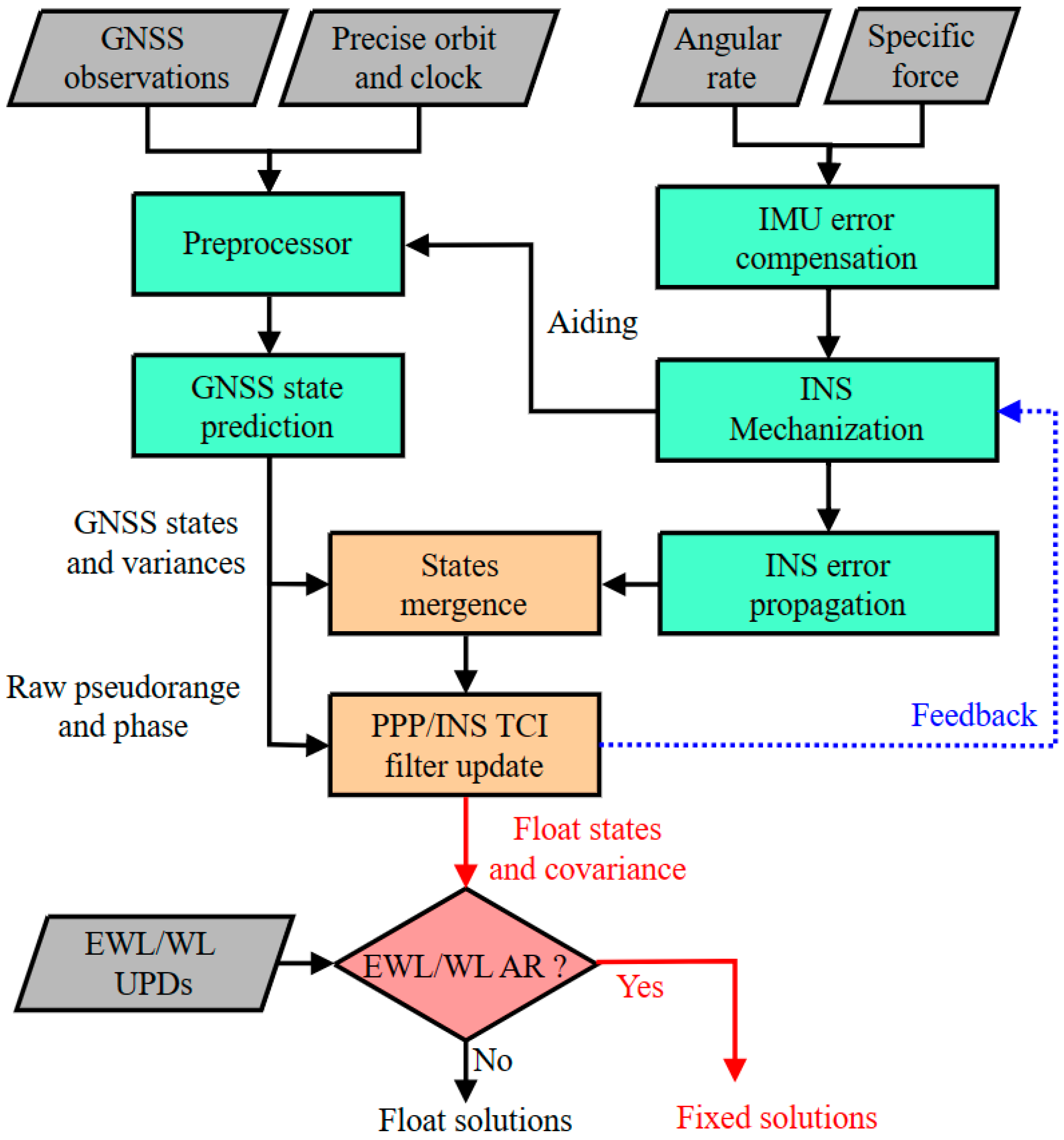
The schematic of the proposed algorithm is presented in Figure 1, consisting of the GNSS module, INS module, fusion module, and ambiguity resolution module. Once the system is initialized, it enters the navigation and filter update phase driven by the INS mechanization. The extended Kalman filter (KF) is employed to fuse the GNSS and IMU sensor measurements to estimate the PPP/INS TCI state. In which, the original GNSS pseudorange and carrier phase observations are responsible for measurement updates to correct the system state. The INS short-term high-precision position is employed to assist in the identification and isolation of GNSS anomaly observations. The GNSS preprocessing includes anomaly pseudorange extraction and carrier phase cycle jump detection. In this study, the latter is implemented based on the well-known TurboEdit method. During a complete GNSS outage, only the INS mechanization and KF time updates are performed, and the measurement updates are dropped.

The estimation of navigation state and float carrier phase ambiguity is captured using measurement updates. Afterwards, the float ambiguity and the corresponding variance are incorporated into the AR module to be resolved and constrained to the estimator, thereby yielding a navigation solution for WLAF. At the same time, the sensor bias of the IMU is simultaneously calibrated for state propagation in the next time step, as shown by the blue arrow in Figure 1.

In practical terms, compared to WL ambiguity-fixed PPP, the attribute of WL ambiguity in PPP/INS-integrated solutions is unchanged so that the WL ambiguity resolution module and strategy can be shared by the PPP estimator and PPP/INS estimator.

4. Experiment Description

To resolve the EWL and WL ambiguities, the multi-frequency GNSS observations from MGEX on DOY 351 in 2020, at 106 stations with 30 s sampling rates, were collected in order to estimate precise EWL and WL UPDs using GREAT-UPD. To assess the performance of our proposed approach, we arranged a vehicle-borne experiment with a multi-GNSS and multi-frequency board (Septentrio AsteRx4) equipped with an antenna (Trimble Zephyr Model 2), a tactical-grade Fiber Optical Gyro (FOG)-IMU (StarNeto XW-GI7660), around Wuhan City in China on 16 December 2020. The specific technical information of the IMU sensors is shown in

Table 1. Technical parameters of the GNSS (Septentrio) and IMU (StarNeto XW-GI7660) sensors.

IMU	Offsets		Random Walk
	Gyro. (°/h)	Acc. (mGal)	Angle (°/$\sqrt{h}$)	Velocity (mg/$\sqrt{h}$)
	0.3	100	0.01	--
GNSS	GPS Signal	BDS Signal	Galileo Signal	Sample Rate
	L1/L2/L5	B1I/B2I/B3I	E1/E5a/E5b	1 Hz

. The illustration of the experimental equipment is presented in Figure 2, and the lever arm between the IMU center and GNSS antenna phase center was accurately measured before the experiment. The time synchronization was carried out at the hardware level to unit timestamps from inertial sensors to GPS time.

The GNSS and IMU measurements were collected at 1 Hz and 200 Hz, respectively. The raw data included two observation periods: the first was from Coordinated Universal Time (UTC) 8:30 to 9:10 in a near urban environment (Traj. A), and the latter was from UTC 9:20 to 9:40 in real urban GNSS-challenged environments (Traj. B). The trajectories of two datasets are displayed on Google Maps in Figure 3. The corresponding travel velocities are shown in Figure 4.

In the data process, the products of the precise orbit, clock, and earth rotation parameterizer (ERP) released by GFZ (German Research Center for Geosciences) were adopted. Pseudorange and carrier phase observations on GPS L1/L2/L5, BDS B1I/B2I/B3I, and Galileo E1/E5a/E5b were employed in an undifferenced and uncombined mode. The weights of the different satellite measurements were assigned according to an elevation-dependent strategy with a prior accuracy of 3 m and 0.03 cycles for pseudorange and carrier phase, respectively. The cutoff elevation angle was preset to 7° to weed out low-quality measurements. In this study, we modeled the residual ionospheric delay as white noise, while the tropospheric wet delay in the zenith direction was modeled as a random walk process with a spectral density of 6 mm/$\sqrt{h}$. The ISBs, IFBs, and ambiguity parameters were described using constant processes. The power spectral densities (PSDs) of attitude and velocity were set to 0.01°/$\sqrt{h}$ and 0.01 mg/$\sqrt{Hz}$, respectively. It should be noted that in order to obtain as many solutions as possible, provided that the number of satellites did not fall below a predetermined minimum, an ambiguity-fixed solution was chosen instead of a float solution, despite the risk of an incorrect resolution.

The reference station instrumented with a Septentrio receiver was placed in an open area close to the trajectory. The reference scheme was computed using the commercial Inertial Explorer (IE) version 8.7 software with a bi-directional smoothed post-processing kinematic (PPK) and INS tightly integrated processing mode [44]. The scheme enabled a centimeter-level accuracy position estimation with an ambiguity resolution of 94.10%. Thus, the ground truth yielded up to an order of magnitude with greater accuracy than the proposed scheme to be assessed.

5. Results and Analysis

Based on the above theoretical analysis and vehicle-borne experiment, the performance of continuous decimeter-level positioning based on WL ambiguity-fixed PPP/INS tight fusion is adequately tested and evaluated. It should be noted that the estimated accuracy of velocity and attitude for the GNSS/INS-integrated system mainly depends on the grade of IMU, whereas the absolute position accuracy is determined by the quality of the carrier phase and ambiguity resolution [30]. Thus, only the performance of positioning is of interest in the proposed method.

5.1. Instantaneous Decimeter-Level Positioning Performance of WLAF PPP

The position differences in Traj. A calculated by the float PPP and proposed WLAF PPP solutions, with respect to the references, are shown in Figure 5. The RMS of position errors is (0.24, 0.15, 0.42) m in the east, north, and up directions for the WLAF PPP, compared to (0.50, 0.22, 0.53) m for float PPP, which suggests improvements of (52.30%, 29.68%, 20.60%) after WL ambiguity resolution is imposed on the float PPP solutions. It should be noted that three re-convergences take place and are marked in light blue shades, owing to the overpasses during the second half of Traj. A. Therefore, both float PPP and WL ambiguity-fixed PPP lack several epochs of solutions and present the re-initializations to varying degrees. Fortunately, the nearly instantaneous decimeter-level positioning is foreseeable, thanks to WL ambiguity resolution, which can be attributed to the super-long wavelength of EWL and WL observations. In particular, the WLAF PPP can significantly shorten the time of convergence and accomplish fast decimeter-level positioning within a few seconds. Taking the vertical direction as an example, single-epoch instantaneous decimeter-level positioning can be easily achieved for WLAF PPP solutions, while re-convergence takes approximately 85 s for float PPP, where “convergence” is defined as the epoch when the accuracy is less than 0.5 m for 30 consecutive epochs.

Moreover, the positioning availability is an invaluable metric for assessing positioning systems, where we define “positioning availability” as the proportion of epochs whose position errors are less than certain thresholds to the total epochs. We, in the contribution, set three threshold levels:

Level 1: less than 1.0 m in the horizontal direction and 1.5 m in the up direction;

Level 2: less than 0.5 m in the horizontal direction and 1.0 m in the up direction;

Level 3: less than 0.3 m in the horizontal direction and 0.5 m in the up direction.

Figure 6 and

Table 2. Availability of positioning at three threshold levels in two processing strategies and the corresponding percentages of improvement.

Availability	Processing Strategies		Improvement
	Float PPP	WLAF PPP
Level 1	90.36%	98.14%	7.78%
Level 2	71.78%	95.25%	32.70%
Level 3	54.58%	85.78%	57.16%

show the positioning availability percentages at three accuracy threshold levels. It can be seen that the availability rate of Level 3 is up to 85.78% for WLAF PPP solutions while it is only 54.58% for float PPP solutions. These statistics suggest the percentages of availability of positioning at three accuracy threshold levels are ameliorated (7.78%, 32.70%, 57.16%) in the WLAF PPP mode, compared to the float PPP solutions. These facts convey that pronounced improvements in availability can be achieved in the WL ambiguity-fixed PPP solutions, even if the GNSS suffers from some irregularities in urban areas.

Nevertheless, even the WLAF PPP will encounter more severe challenges in more complex and harsh environments due to the limitation and fragility of the GNSS. A close look at the number series of available satellites from Traj. B in Figure 3 exposes that there are only few available satellites (less than 10) in certain environments where there are many buildings and trees, which significantly degrades the continuity and availability of PPP solutions. Comparing the references, Figure 7 depicts the positioning errors series of Traj. B for all three components in float PPP and WLAF PPP modes. The RMS of position bias drops from (1.61, 1.04, 1.47) m for the float PPP solutions to (1.49, 0.98, 1.19) m for the WLAF PPP solutions, with an accuracy improvement of (7.50%, 5.75%, 18.86%) in the east, north, and up directions, respectively, as presented in

Table 3. RMSs of position bias of the float PPP and WLAF PPP of Traj. B relative to the reference.

RMS (m)	East	North	Up
Float PPP	1.61	1.04	1.47
WLAF PPP	1.49	0.98	1.19
Improv. (%)	7.50	5.75	18.86

. However, the rate of availability is only 58.42% for WL ambiguity-fixed PPP solutions at Level 2. In spite of the support of WL ambiguity resolution, a single positioning system still cannot bring about the desired and acceptable consequence and rigorously fulfill the required accuracy and availability in autonomous driving during the occlusions from the structures and crossovers blockage.

5.2. INS Aiding Effect on Continuous Decimeter-Level Positioning

Figure 8 demonstrates the positioning differences in WLAF PPP and WLAF PPP/INS solutions for both trajectories. As expected, the positioning accuracy, continuity, and reliability are considerably enhanced in WLAF PPP/INS solutions, compared to the WLAF PPP-only solutions. The statistics of position RMS are calculated and presented in

Table 4. RMSs of position bias of the WLAF PPP- and WLAF PPP/INS-integrated solutions of the two trajectories relative to the reference.

RMS (m)	Traj. A			Traj. B
	East	North	Up	East	North	Up
WLAF PPP	0.24	0.15	0.42	1.49	0.98	1.19
WLAF PPP/INS	0.08	0.09	0.21	0.19	0.09	0.57
Improv. (%)	67.78	40.26	50.48	87.27	91.14	51.93

for the two trajectories. For the first trajectory, the RMS of position errors is (0.08, 0.09, 0.21) m in the east, north, and up directions for the WLAF PPP/INS, compared to (0.24, 0.15, 0.42) m for the WLAF PPP solutions. The RMS of position bias for the second trajectory drops significantly from (1.49, 0.98, 1.19) m for the WLAF PPP solutions to (0.19, 0.09, 0.57) m for the WLAF PPP/INS solutions in all three directions, with an improvement of (87.27%, 91.14%, 51.93%) when compared to the WLAF PPP solutions. The positioning performance of both experiments is significantly ameliorated, especially for Traj. B where the observation condition is more severe and harsh.

Figure 9 and

Table 5. The availability rate of positioning at three threshold levels in float PPP, WLAF PPP, float PPP/INS, and WLAF PPP/INS modes.

Availability Rate	Traj. A			Traj. B
	Level 1	Level 2	Level 3	Level 1	Level 2	Level 3
Float PPP	90.36%	71.78%	54.58%	74.54%	43.91%	13.47%
WLAF PPP	98.14%	95.25%	85.78%	77.21%	53.78%	27.58%
Float PPP/INS	96.85%	93.30%	87.64%	95.94%	89.85%	75.09%
WLAF PPP/INS	99.14%	98.31%	94.55%	96.49%	93.91%	76.48%

further demonstrate that the rates of availability of positioning of both trajectories at three threshold levels are significantly improved with the assistance of the INS. Taking a typical accuracy of 0.5 m in autonomous driving as an example, the percentage of positioning availability of the second track at Level 2 for the WLAF PPP/INS is 93.91%, as opposed to 89.85% for the float PPP/INS, 53.78% for the WLAF PPP, and 43.91% for the float PPP solutions. Moreover, for the demand for higher precision, Level 3, the availability rate of positioning of the WLAF PPP/INS tightly coupled solutions is still up to 76.48%, whereas it is only 27.58% for the WLAF PPP-only solutions.

In addition, in order to intuitively exhibit the contribution of the INS on positioning continuity, the trajectories of two typical scenes are displayed in Figure 10. The directions of movement are denoted by red arrows. The yellow, red, blue, and green lines stand for the solutions of the float PPP, WLAF PPP, WLAF PPP/INS, and reference benchmark. The colored dots on the lines stand for the corresponding positioning solutions. Figure 10a shows that with the assistance of the INS, the continuity of position estimation can be perfectly maintained, even in a tunnel where the GNSS is completely interrupted, and the decimeter-level positioning can be obtained instantaneously after the GNSS signals are relocked. Two snapshots in Figure 10b show another typical scenario, where the GNSS frequently encounters occlusions in a wooded environment. It should be noted that to avoid the overlay among four tracks, the float PPP and WLAF PPP solutions are shown in the top panel of snapshot b, while the PPP/INS and reference solutions are shown in the bottom. The trajectory determined by the WLAF PPP/INS tightly coupled positioning coincides well with the reference benchmarks with very little deviations. In contrast, the float PPP and WLAF PPP solutions tend to have significant deviations and even lack during GNSS-challenged periods. Overall, for both trajectories, great improvements are achieved in terms of positioning availability and continuity through WL ambiguity-fixed PPP/INS-integrated solutions, as opposed to corresponding PPP-only solutions.

To further investigate the role of WL ambiguity resolution in PPP/INS tightly coupled integration, a few simulated full GNSS outages are carried out. The full outage, namely gap, is here defined to be the complete interruption of all GNSS observations to the integrated navigation system in some scenarios, such as long tunnels and continuous occlusion overpasses. The constraint effect of the INS is dramatically weakened for the PPP/INS tightly coupled solutions under the above circumstances, owing to degraded positioning accuracy caused by the long-term independent mechanization of the INS. Therefore, four full GNSS outages of different durations are simulated individually at the same epoch point. Figure 11 depicts the position error time series of WLAF PPP, float PPP/INS, and WLAF PPP/INS tightly integrated solutions during the GNSS outages. It can be noted that in short-term simulated outages (e.g., 10 s and 30 s), the continuous position information of the INS makes the tightly coupled solutions more stable than the WLAF PPP-only solutions. However, as the outage time increases (e.g., 60 s and 90 s), whether it is float PPP/INS or WLAF PPP/INS solutions, the contribution of the INS to the integrated algorithm gradually weakens. Fortunately, when the GNSS signals are relocked, due to the benefit of WL ambiguity resolution, the WLAF PPP/INS tightly coupled solutions can realize the decimeter-level positioning faster than the float PPP/INS solutions. In the 60 s full GNSS outage simulated test, the convergence time of the position error at Level 3 is only 31 s for the WLAF PPP/INS solutions, while that of the float PPP/INS solutions is 74 s.

6. Discussion

In view of the slow initialization of PPP-based tightly coupled schemes in urban scenarios and the difficulty in narrow-lane ambiguity resolution, this study proposes a tightly coupled approach for the PPP/INS, exploiting triple-frequency observations. Two of the advantages ensure that the proposed system can achieve stable and continuous high-precision positioning. Firstly, the ambiguity can be resolved instantaneously by virtue of the long wavelength of the ultra-wide lane and wide lane combination, which ensures that the system can perform fast initialization in spite of frequent disturbances. Secondly, the tightly integrated design allows the short-term high accuracy of the INS to be employed to bridge the positioning of GNSS interruption scenarios and further accelerate the re-positioning of the signal after recapture, thus enabling continuous position estimation. As illustrated in Figure 11, the proposed system is capable of considerably shorter convergence times compared to conventional methods, which offers a new possibility for time-critical applications.

In the face of long-term satellite signal loss, the proposed system still struggles to perform high-precision navigation tasks during the pure INS prediction phase, which is a common problem with INS-based positioning approaches. The integration of additional sensors is therefore beneficial in alleviating this deficiency. Furthermore, the method proposed in this paper requires a hardware capable of receiving and demodulating measurements at multiple frequencies. With advances in manufacturing processes and cost control, it is foreseeable that it will be accessible to the mass market in the near future.

7. Conclusions

In this paper, we established a triple-frequency PPP/INS tightly coupled positioning system, in which under the combined effect of (extra-) wide-lane ambiguity resolution and an INS, continuous decimeter-level positioning could be obtained without difficulty, utilizing GPS/BDS/Galileo triple-frequency observations. After a detailed and rigorous analysis of the mathematical algorithm, a PPP/INS tightly coupled approach with WL ambiguity resolution was presented. To assess the positioning performance of the proposed system, two sets of vehicle-borne data in urban environments were processed.

Compared to float PPP, the introduction of WL ambiguity resolution could dramatically ameliorate position accuracy and achieve decimeter-level positioning within a few seconds. Due to the virtue of their long wavelengths, the EWL and WL ambiguities could be resolved easily, which provided the basis for instantaneous and precise positioning. The RMS of position bias was (0.24, 0.15, 0.42) m in the east, north, and up directions with the improvements of (52.30%, 29.68%, 20.60%) after WL ambiguity resolution was imposed on the float PPP solutions in urban experiments. The percentage of positioning accuracy better than 0.3 m in horizontal directions and 0.5 m in vertical direction was up to 85.78% for the WLAF PPP solutions of the total epochs, which was only 54.58% for the float PPP solutions.

For the position estimation of WLAF PPP/INS tightly coupled integration, compared to the WLAF PPP solutions, dramatic improvements of (67.78%, 40.26%, 50.48%) and (87.27%, 91.14%, 51.93%) could be attained for both experiments, even if the GNSS suffered from frequent and serious challenges in urban areas. In the second set of experiments where the environment was more severe, the percentage of positioning accuracy was better than 0.3 m in horizontal directions and 0.5 m in the vertical direction, still reaching 76.48% of epochs, as opposed to only 27.58% and 13.47% for the WLAF PPP and float PPP solutions, respectively. In addition, in some typical scenarios, such as tunnels and wooded areas, the positioning continuity of the integrated system could be maintained smoothly when compared to the WLAF PPP-only solutions. Moreover, after the GNSS was completely out of lock for about one minute, the WLAF PPP/INS-integrated system showed better robustness in maintaining decimeter-level positioning than the float PPP/INS solutions.

In this study, however, continuous decimeter-level precise positioning was tricky and troublesome for a peculiarly long period of GNSS outages, affected by the grade of the inertial sensor and observation scenarios. Therefore, we have to introduce multi-sensor information, such as cameras and lidars, to boost continuous positioning capability, which will be the focus of future research.

References

- Kuutti, S.; Fallah, S.; Katsaros, K.; Dianati, M.; Mccullough, F.; Mouzakitis, A. A survey of the 34 state-of-the-art localization techniques and their potentials for autonomous vehicle applications. IEEE Internet Things J. 2018, 5, 829–846. [Google Scholar] [CrossRef]
- Reid, T.G.; Houts, S.E.; Cammarata, R.; Mills, G.; Agarwal, S.; Vora, A.; Pandey, G. Localization requirements for autonomous vehicles. arXiv 2019, arXiv:1906.01061. [Google Scholar] [CrossRef]
- Kassas, Z.M.; Closas, P.; Gross, J. Navigation systems panel report navigation systems for autonomous and semi-autonomous vehicles: Current trends and future challenges. IEEE Aerosp. Electron. Syst. Mag. 2019, 34, 82–84. [Google Scholar] [CrossRef]
- Joubert, N.; Reid, T.G.; Noble, F. Developments in modern GNSS and its impact on autonomous vehicle architectures. In Proceedings of the 2020 IEEE Intelligent Vehicles Symposium (IV), Las Vegas, NV, USA, 19 October–13 November 2020; pp. 2029–2036. [Google Scholar]
- Takasu, T.; Yasuda, A. Development of the low-cost RTK-GPS receiver with an open source program package RTKLIB. In Proceedings of the International Symposium on GPS/GNSS, International Convention Center Jeju Korea, Seogwipo-si, Korea, 4–6 November 2009; Volume 1, pp. 1–6. [Google Scholar]
- He, H.; Li, J.; Yang, Y.; Xu, J.; Guo, H.; Wang, A. Performance assessment of single-and dual-frequency BeiDou/GPS single-epoch kinematic positioning. GPS Solut. 2014, 18, 393–403. [Google Scholar] [CrossRef]
- Odolinski, R.; Teunissen, P.; Odijk, D. Combined GPS+ BDS for short to long baseline RTK positioning. Meas. Sci. Technol. 2015, 26, 045801. [Google Scholar] [CrossRef]
- Zumberge, J.; Heflin, M.; Jefferson, D.; Watkins, M.; Webb, F. Precise point positioning for the efficient and robust analysis of GPS data from large networks. J. Geophys. Res. Solid Earth 1997, 102, 5005–5017. [Google Scholar] [CrossRef]
- Ge, M.; Gendt, G.; Rothacher, M.A.; Shi, C.; Liu, J. Resolution of GPS carrier-phase ambiguities in precise point positioning (PPP) with daily observations. J. Geod. 2008, 82, 389. [Google Scholar] [CrossRef]
- Li, X.; Zhang, X.; Ren, X.; Fritsche, M.; Wickert, J.; Schuh, H. Precise positioning with current multi-constellation global navigation satellite systems: GPS, GLONASS, Galileo and BeiDou. Sci. Rep. 2015, 5, 8328. [Google Scholar] [CrossRef]
- Henkel, P.; Gunther, C. Precise point positioning with multiple Galileo frequencies. In Proceedings of the 2008 IEEE/ION Position, Location and Navigation Symposium, Monterey, CA, USA, 5–8 May 2008; pp. 592–599. [Google Scholar]
- Gu, S.; Lou, Y.; Shi, C.; Liu, J. BeiDou phase bias estimation and its application in precise point positioning with triple-frequency observable. J. Geod. 2015, 89, 979–992. [Google Scholar] [CrossRef]
- Li, P.; Zhang, X.; Ge, M.; Schuh, H. Three-frequency BDS precise point positioning ambiguity resolution based on raw observables. J. Geod. 2018, 92, 1357–1369. [Google Scholar] [CrossRef]
- Li, X.; Li, X.; Liu, G.; Feng, G.; Yuan, Y.; Zhang, K.; Ren, X. Triple-frequency PPP ambiguity resolution with multi-constellation GNSS: BDS and Galileo. J. Geod. 2019, 93, 1105–1122. [Google Scholar] [CrossRef]
- Jonkman, N.; Teunissen, P.; Joosten, P.; Odijk, D. GNSS long baseline ambiguity resolution: Impact of a third navigation frequency. In Geodesy Beyond 2000: The Challenges of the First Decade IAG General Assembly Birmingham, July 19–30, 1999; Springer: Berlin/Heidelberg, Germany, 2000; pp. 349–354. [Google Scholar]
- Li, B.; Li, Z.; Zhang, Z.; Tan, Y. ERTK: Extra-wide-lane RTK of triple-frequency GNSS signals. J. Geod. 2017, 91, 1031–1047. [Google Scholar] [CrossRef]
- Li, P.; Jiang, X.; Zhang, X.; Ge, M.; Schuh, H. GPS+ Galileo+ BeiDou precise point positioning with triple-frequency ambiguity resolution. GPS Solut. 2020, 24, 78. [Google Scholar] [CrossRef]
- Feng, Y.; Li, B. Wide area real time kinematic decimetre positioning with multiple carrier GNSS signals. Sci. China Earth Sci. 2010, 53, 731. [Google Scholar] [CrossRef]
- Geng, J.; Guo, J.; Chang, H.; Li, X. Toward global instantaneous decimeter-level positioning using tightly coupled multi-constellation and multi-frequency GNSS. J. Geod. 2019, 93, 977–991. [Google Scholar] [CrossRef]
- Li, X.; Li, X.; Liu, G.; Yuan, Y.; Freeshah, M.; Zhang, K.; Zhou, F. BDS multi-frequency PPP ambiguity resolution with new B2a/B2b/B2a+ b signals and legacy B1I/B3I signals. J. Geod. 2020, 94, 107. [Google Scholar] [CrossRef]
- Petovello, M.G. Real-Time Integration of a Tactical-Grade IMU and GPS for High-Accuracy Positioning and Navigation; Citeseer: Princeton, NJ, USA, 2003. [Google Scholar]
- Zhang, Y.; Gao, Y. Performance analysis of a tightly coupled kalman filter for the integration of un-differenced GPS and inertial data. In Proceedings of the 2005 National Technical Meeting of The Institute of Navigation, San Diego, CA, USA, 24–26 January 2005; pp. 270–275. [Google Scholar]
- Xia, X.; Meng, Z.; Han, X.; Li, H.; Tsukiji, T.; Xu, R.; Zhang, Z.; Ma, J. Automated Driving Systems Data Acquisition and Processing Platform. arXiv 2022, arXiv:2211.13425. [Google Scholar]
- Xia, X.; Hashemi, E.; Xiong, L.; Khajepour, A. Autonomous Vehicle Kinematics and Dynamics Synthesis for Sideslip Angle Estimation Based on Consensus Kalman Filter. IEEE Trans. Control Syst. Technol. 2022, 31, 179–192. [Google Scholar] [CrossRef]
- Gao, L.; Xiong, L.; Xia, X.; Lu, Y.; Yu, Z.; Khajepour, A. Improved vehicle localization using on-board sensors and vehicle lateral velocity. IEEE Sens. J. 2022, 22, 6818–6831. [Google Scholar] [CrossRef]
- Liu, W.; Xia, X.; Xiong, L.; Lu, Y.; Gao, L.; Yu, Z. Automated vehicle sideslip angle estimation considering signal measurement characteristic. IEEE Sens. J. 2021, 21, 21675–21687. [Google Scholar] [CrossRef]
- Xiong, L.; Xia, X.; Lu, Y.; Liu, W.; Gao, L.; Song, S.; Yu, Z. IMU-based automated vehicle body sideslip angle and attitude estimation aided by GNSS using parallel adaptive Kalman filters. IEEE Trans. Veh. Technol. 2020, 69, 10668–10680. [Google Scholar] [CrossRef]
- Kim, J.; Jee, G.I.; Lee, J.G. A complete GPS/INS integration technique using GPS carrier phase measurements. In Proceedings of the IEEE 1998 Position Location and Navigation Symposium (Cat. No. 98CH36153), Atlanta, GA, USA, 20–23 April 1996; pp. 526–533. [Google Scholar]
- Groves, P.D. Principles of GNSS, inertial, and multisensor integrated navigation systems, [Book review]. IEEE Aerosp. Electron. Syst. Mag. 2015, 30, 26–27. [Google Scholar] [CrossRef]
- Liu, S.; Sun, F.; Zhang, L.; Li, W.; Zhu, X. Tight integration of ambiguity-fixed PPP and INS: Model description and initial results. GPS Solut. 2016, 20, 39–49. [Google Scholar] [CrossRef]
- Scherzinger, B.M. Precise robust positioning with inertial/GPS RTK. In Proceedings of the 13th International Technical Meeting of the Satellite Division of The Institute of Navigation (ION GPS 2000), Salt Lake City, UT, USA, 19–22 September 2000; pp. 155–162. [Google Scholar]
- Kjørsvik, N.; Gjevestad, J.; Brøste, E.; Gade, K.; Hagen, O. Tightly coupled precise point positioning and inertial navigation systems. In Proceedings of the International Society for Photgrammetry and Remote Sensing European Calibration and Orientation Workshop, Casteldefels, Spain, 10–12 February 2010. [Google Scholar]
- Abd Rabbou, M.; El-Rabbany, A. Integration of multi-constellation GNSS precise point positioning and MEMS-based inertial systems using tightly coupled mechanization. Positioning 2015, 6, 81. [Google Scholar] [CrossRef]
- Gao, Z.; Zhang, H.; Ge, M.; Niu, X.; Shen, W.; Wickert, J.; Schuh, H. Tightly coupled integration of multi-GNSS PPP and MEMS inertial measurement unit data. GPS Solut. 2017, 21, 377–391. [Google Scholar] [CrossRef]
- Saastamoinen, J. Contributions to the theory of atmospheric refraction. Bull. Géodésique (1946–1975) 1972, 105, 279–298. [Google Scholar] [CrossRef]
- Böhm, J.; Niell, A.; Tregoning, P.; Schuh, H. Global Mapping Function (GMF): A new empirical mapping function based on numerical weather model data. Geophys. Res. Lett. 2006, 33, L07304. [Google Scholar] [CrossRef]
- Pan, L.; Zhang, X.; Li, X.; Liu, J.; Li, X. Characteristics of inter-frequency clock bias for Block IIF satellites and its effect on triple-frequency GPS precise point positioning. GPS Solut. 2017, 21, 811–822. [Google Scholar] [CrossRef]
- Thoelert, S.; Steigenberger, P.; Montenbruck, O.; Meurer, M. Signal analysis of the first GPS III satellite. GPS Solut. 2019, 23, 92. [Google Scholar] [CrossRef]
- Li, X.; Han, X.; Li, X.; Liu, G.; Feng, G.; Wang, B.; Zheng, H. GREAT-UPD: An open-source software for uncalibrated phase delay estimation based on multi-GNSS and multi-frequency observations. GPS Solut. 2021, 25, 66. [Google Scholar] [CrossRef]
- Li, X.; Liu, G.; Li, X.; Zhou, F.; Feng, G.; Yuan, Y.; Zhang, K. Galileo PPP rapid ambiguity resolution with five-frequency observations. GPS Solut. 2020, 24, 24. [Google Scholar] [CrossRef]
- Dong, D.N.; Bock, Y. Global positioning system network analysis with phase ambiguity resolution applied to crustal deformation studies in California. J. Geophys. Res. Solid Earth 1989, 94, 3949–3966. [Google Scholar] [CrossRef]
- Shin, E.H. Estimation Techniques for Low-Cost Inertial Navigation. Ph.D. Thesis, The University of Calgary, Calgary, AB, Canada, 2005. [Google Scholar]
- Brown, R.; Hwang, P. Introduction to Random Signals and Applied Kalman Filtering; John Wiley & Sons Inc.: New York, NY, USA, 1992; p. 512. [Google Scholar]
- NovAtel. Inertial Explorer, version 8.9; NovAtel: Calgary, AB, Canada, 2022. [Google Scholar]
Figure 1.
Flowchart of WL ambiguity-fixed PPP/INS tightly coupled integration. After the float solution is obtained, the corresponding states and covariance are employed for the ambiguity solution. Once the ambiguity is successfully resolved, then the WLAF PPP/INS solution is output, as shown by the red arrow in the figure.
Figure 2.
Snapshot of the experimental platform.
Figure 3.
Two trajectories of the vehicle-borne experiment in Wuhan City, China, on 16 December 2020. The number of available GPS/BDS/Galileo satellites and corresponding Position Dilution Of Precision (PDOP) values are shown in the bottom of the corresponding panel.
Figure 4.
The vehicle travel speed sequences for the two experiments with Traj. A on the left and Traj. B on the right.
Figure 5.
Position differences in float PPP (red dots) and WLAF PPP (blue dots) solutions in the east, north, and up directions. The results were acquired from Traj. A. RMSs of two solutions are shown on the upper and lower sides of the sequence in corresponding colors. The small panel of the second interruption in the vertical direction is shown on the right.
Figure 6.
The percentage of positioning availability at three threshold levels in float PPP and WLAF PPP modes, which are drawn with the colors red and blue, respectively.
Figure 7.
Position differences in float PPP (red dots) and WLAF PPP (blue dots) solutions in the east, north, and up directions for Traj. B. The green horizontal dashed lines on the top and middle indicate a range of ±0.5 m; whereas, the dashed line on the bottom indicates ±1.0 m, which represents the Level 2 availability limit.
Figure 8.
Position error sequences of WLAF PPP solutions (red dots) and WLAF PPP/INS-integrated solutions (green dots) in the east, north, and up directions. The results are calculated from Traj. A and Traj. B, shown in the top and bottom panels, respectively. The purple dashed horizontal line within the first two rows of each panel indicates a range of ±0.3 m, while the dashed line within the third row indicates ±0.5 m, which is representative of the third level of position availability boundaries.
Figure 9.
The availability rate of positioning at three threshold levels in float PPP, WLAF PPP, float PPP/INS, and WLAF PPP/INS modes, drawn with the red, blue, cyan, and green columns, respectively. The availability rates of positioning of Traj. A are displayed in the top of the panel, while those of Traj. B are displayed in the bottom of the panel, stuffed with slashes and backslashes, respectively.
Figure 10.
Snapshots of vehicle-borne trajectory in two typical scenarios: a tunnel (a) and wooded areas (b), overlaid in Google Maps. The two tracks escorted by the dashed red polygons represent the above two scenes.
Figure 11.
Position bias sequences in east, north, and up directions during four GNSS–simulated outages. The top, middle, and bottom panels stand for the WLAF PPP, float PPP/INS, and WLAF PPP/INS, respectively. The panels from left to right denote different interruption durations, namely gaps marked in the shades. The arrow points to the epoch where the position error converges to Level 3, and the corresponding convergence time is placed next to it.