Abstract
Accurate precipitation measurements are essential for understanding hydrological processes in high-altitude regions. Conventional gauge measurements often yield large underestimations of actual precipitation, prompting the development of statistical methods to correct the measurement bias. However, the complex conditions at high altitudes pose additional challenges to the statistical methods. To improve the correction of precipitation measurements in high-altitude areas, we selected the Yakou station, situated at an altitude of 4147 m on the Tibetan plateau, as the study site. In this study, we employed the machine learning method XGBoost regression to correct precipitation measurements using meteorological variables and remote sensing data, including Global Satellite Mapping of Precipitation (GSMaP), Integrated Multi-satellitE Retrievals for GPM (IMERG) and Climate Hazards Group InfraRed Precipitation with Station data (CHIRPS). Additionally, we examined the transferability of this method between different stations in our study site, Norway, and the United States. Our results show that the Yakou station experiences a large underestimation of precipitation, with a magnitude of 51.4%. This is significantly higher than similar measurements taken in the Arctic or lower altitudes. Furthermore, the remote sensing precipitation datasets underestimated precipitation when compared to the Double Fence Intercomparison Reference (DFIR) precipitation observation. Our findings suggest that the machine learning method outperformed the traditional statistical method in accuracy metrics and frequency distribution. Introducing remote sensing data, especially the GSMaP precipitation, could potentially replace the role of in situ wind speed in precipitation correction, highlighting the potential of remote sensing data for correcting precipitation rather than in situ meteorological observation. Moreover, our results indicate that the machine learning method with remote sensing data demonstrated better transferability than the traditional statistical method when we cross-validated the method with sites located in different countries. This study offers a promising strategy for obtaining more accurate precipitation measurements in high-altitude regions.
1. Introduction
Accurate in situ precipitation measurements are important for assessing the hydrological impacts of climate change, determining water resource availability, estimating and forecasting flood risk, and understanding the Earth’s energy balance. Accurate measurements of precipitation at high altitudes become even more necessary. These areas, such as the Tibetan Plateau, supplying water resources for a wide range of downstream regions, have high spatiotemporal precipitation variability but with few precipitation gauges [1]. These gauges have obvious measurement bias, limiting their capacity to validate the spatially distributed precipitation datasets.
Solid evidence shows that true precipitation has been underestimated in high wind speed conditions, especially in high mountain areas [2,3]. For instance, Sugiura et al. [4] indicated that the catch ratios of the gauges in Canada, Russia, and the United States range from 53.9 to 67.6%. Jia et al. [5] found that solid precipitation was underestimated by 13% on a glacier at a high altitude. The primary reason for this underestimation is that gauge instruments cannot accurately capture precipitation at high altitudes. When high wind conditions occur in the vicinity of a gauge, the gauge collects less precipitation than what actually fell. Additionally, the precipitation that falls into the gauge may evaporate before it can be measured. Precipitation gauges can also collect less precipitation than what actually fell due to factors such as gauge design, clogging, or icing. The Double Fence Intercomparison Reference (DFIR) was designed to minimize the under-catch of precipitation [6] and was typically used as the actual value of precipitation in correcting other instruments.
Various correction methods have been developed to address the underestimation of precipitation measurements. Correcting precipitation measurements requires consideration of several factors, such as the type of instruments used, the meteorological conditions of the measurement site, and the period for which the data were collected. Statistical correction methods have been developed by the World Meteorological Organization (WMO) to account for wind effects, evaporation loss, and gauge under-catch since the last century [7]. These methods have been improved over time to apply in Siberian regions [8], Arctic regions [9,10], and western Canada [11]. With the advancement of new precipitation instruments such as the Geono T200B, WMO conducted a Solid Precipitation Intercomparison Experiment (WMO-SPICE) to cover automatic gauges but not the traditional manual instruments in the earlier comparison [12]. Based on the measurements, Wolff et al. [13] presented a continuous adjustment function for correcting wind-induced loss of solid precipitation based on data from a Norwegian field study. Kochendorfer et al. [14] simplified the transfer function to an exponential formula using wind speed and air temperature as inputs. This transfer function method (TFM) was examined [15] and applied to other regions. For example, Smith et al. [16] used the transfer function to adjust the wind-induced under-catch of solid precipitation in the Climate Change Canada Automated Surface Observation Network (CCCASON) and provides access to an hourly adjusted data set. Using the TFM method recalibrated with a local dataset, Zhao et al. [17] corrected the precipitation observation in the Qilian Mountains in Northwest China.
These studies have shown that the statistical TFM method can be used for correcting precipitation measurements in high wind conditions. However, the appropriate methods may differ depending on the type of precipitation gauge and the measurement location. For instance, Sugiura et al. [4] have argued that the WMO correction equations are unsuitable for high wind speeds in high-latitude regions. Similarly, Smith et al. [18] found that the performance of transfer functions varies greatly by site, suggesting caution in their application. Zhao et al. [17] suggested that the transfer functions should be fitted to the local dataset. Additionally, we also noticed that current precipitation measurement correction only includes a few meteorological variables, such as air temperature and wind speed, while others, such as radiation and ground moisture, are not considered. It remains unclear whether these meteorological variables can contribute to precipitation measurement correction.
The precipitation correction methods described above are mainly intended for ground-based measurement instruments. While these methods can provide more accurate precipitation estimates for a few stations, they cannot account for larger areas with limited coverage, such as high-altitude regions. In recent years, remotely sensed (RS) precipitation products have been developed rapidly and have been validated and applied in many areas. Satellite precipitation uses near-infrared, passive microwave, and multi-sensor joint algorithms to invert precipitation, providing precipitation information that covers a wide range of terrain, including high altitudes. The current mainstream satellite precipitation products include Tropical Rainfall Measuring Mission (TRMM) [19], CPC MORPHing technique (CMORPH) [20], Global Satellite Mapping of Precipitation (GSMaP) [21], and Integrated Multi-satellitE Retrievals for GPM (IMERG) [22], among others. However, evaluating remotely sensed precipitation products remains challenging due to the lack of accurate ground-based precipitation measurement equipment at high altitudes, such as the DFIR. On the other hand, remotely sensed precipitation products provide data information different from ground-based observations. Can this remotely sensed information be used to make precipitation corrections that differ from traditional methods? This is a promising direction for precipitation measurement correction under the rapid development of remote sensing technology.
As mentioned above, combining in situ meteorological variables with remotely sensed precipitation datasets may improve the accuracy of in situ precipitation measurements. Machine learning methods have emerged as a promising approach to accomplish this task. These methods have strong data generalization capabilities and have successfully fused precipitation data and corrected remotely sensed precipitation. For instance, Gagne et al. [23] applied multiple machine learning algorithms to correct precipitation forecasts from the Storm Scale Ensemble Forecast system, which resulted in improved reliability and skill of the forecasts compared to the original ensemble. Similarly, Wang et al. [24] suggested that customized deep learning methods can effectively correct precipitation with fine spatial and temporal resolutions. These results suggested that machine learning can remove negative biases and placement mistakes in precipitation forecasts, thereby improving flood and hydrological process predictions. However, it is important to note that these machine-learning methods only correct spatially distributed precipitation products and do not target in situ measurements.
In summary, while efforts have been made to correct wind-induced precipitation, challenges remain when correcting precipitation measurements at high altitudes. Currently, precipitation measurement corrections are limited to a few stations with so-called “true value” observations, such as the DFIR. There is a lack of extension of these corrections to more sites equipped with only common precipitation measurement instruments, such as the T200B. In high-altitude areas, it is even more crucial to utilize additional meteorological variables and remote sensing data to ensure the stability and accuracy of precipitation correction due to the extreme scarcity of meteorological stations. To improve the correction of precipitation measurements in high-altitude areas, we employed machine learning to correct precipitation measurements using additional meteorological variables and remote sensing data. Furthermore, we assessed the transferability of this machine learning method among different stations in our study site and in Norway and the United States.
2. Data and Methods
2.1. Study Site and Data
The Yakou station, a high-altitude site in the northwestern Tibetan plateau (4147 m, 100.243E, 38.014N), was chosen as the study area (Figure 1). The system is located on a mountain peak with a seasonal snowpack. The underlying is a sparse alpine meadow of less than 10 cm, mixed with a cold desert. The maximum wind speed would exceed 10 m/s. The average air temperature is −4.8 °C, the average relative humidity is 59.9%, and the average atmospheric pressure is 612.7 hPa. Snowfall frequently occurs, but the accumulated snowpack is usually less than 30 cm [25].
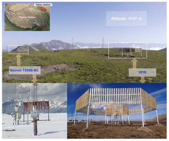
Figure 1.
The Yakou station map. The figure shows the location of the Yakou station at the Tibetan plateau (the red dot), the relative positions, and close-up photos of the precipitation instruments (the T200B and DFIR).
We constructed a Double Fence Intercomparison Reference (DFIR) precipitation observation system according to WMO standards. The system includes double fences to prevent under-measurement of precipitation, and a T200B instrument with three sensors was installed at the center of the fences. This study used the DFIR observation as the true precipitation measurements, as suggested in numerous previous studies [14,17].
For comparison, a Geonor T200B Precipitation instrument was installed near the DFIR, about 20 m away. This T200B also has three weighing sensors and is the same model used in the DFIR. The DFIR and T200B data were preprocessed using a low-pass filtering method to exclude coarse differences, and the cumulative precipitation weight was converted to precipitation per unit time step, following the method of Pan et al. [11]. The detailed introduction for other observations can be found in the previous paper [26].
The selected data period was from 21 September 2016 to 31 August 2020. We preprocessed the DFIR and T200B data into time intervals of 1 h, 6 h, and one day to compare the performance of the machine learning method on different time intervals. For each case of different time intervals, we divided the study period into two halves. The first half was for training the model, and the second half was for prediction or validation.
Snow depth, soil temperature, and moisture data were filtered to remove excessive noise. The details of the meteorological observations used in the machine learning method are listed in Table 1.

Table 1.
The meteorological variables and remote sensing data used in this study. The temporary and spatial resolutions are listed for the remote sensing data. The temporary resolutions are listed for the data on the Yakou site.
For validating the transfer capacity of the machine learning method, we also used the precipitation data from a Norway station and a United States station, which was published in the paper [14].
Remote Sensing Precipitation
We used remotely sensed precipitation datasets from IMERG, GSMaP, and Climate Hazards Group InfraRed Precipitation with Station data (CHIRPS). The information of the three remote sensing datasets is listed in Table 1. IMERG is a Level 3 product that is part of the Global Precipitation Measurement (GPM) program, which is the next-generation global satellite observation initiative of the National Aeronautics and Space Administration (NASA) and the Japan Aerospace Exploration Agency (JAXA) [22]. The GPM carries the GPM Microwave Imager (GMI), the Visible and Infrared Scanner (VIRS), and the Dual-frequency Precipitation Radar (DPR), with the latter being able to detect internal cloud structures better and improve precipitation information acquisition. IMERG includes the IMERG-E, IMERG-L, and IMERG-F products, with lag times of 4 h, 12 h, and 4 months, respectively. IMERG-F, one of the precipitation products used in this study, was corrected using the Global Precipitation Climatology Centre (GPCC) monthly rainfall observation.
GSMaP is a high spatiotemporal resolution precipitation product developed by the Japan Science Technology Agency (JST) and JAXA, which integrated observation information from multiple microwave sensors such as GMI, TMI, AMSU-A, AMSR2, and infrared observation information [21]. The product includes the microwave-IR combined product (GSMaP-MVK), the near-real-time product (GSMaP-NRT), and the gauge-calibrated rainfall product (GSMaP-Gauge). GSMaP-Gauge was used in this study by combining the daily observed precipitation of the Climate Prediction Center (CPC) based on GSMaP-MVK.
CHIRPS is a precipitation product developed by the United States Geological Survey and the Climate Hazards Group, which combines infrared cold cloud duration measurements, satellite imagery, and observations from multiple sources to provide a long-time series and high-resolution precipitation product for climate change analysis and drought monitoring research [27]. The CHIRPS v2.0 precipitation product was used in this study.
The remotely sensed data presented here have time scales of 0.5 H and 1 H. Therefore, to unify the time scales of remote sensing and ground observation data, we resampled them to daily data when performing cross-comparisons of remotely sensed precipitation in this study.
2.2. Method
We aim to correct the T200B precipitation measurements using a machine learning method, in which relevant meteorological variables are selected (Figure 2). After selecting the key features (meteorological variables), the hyper-parameters were calibrated, and the machine learning method was trained to validate the performance of the precipitation correction. Remotely sensed precipitation was also incorporated into the machine learning method to explore whether the RS data can improve precipitation correction. Finally, after building and examining the machine-learning model at the Yakou station, we also examined the transferability of the machine-learning method to other sites worldwide, such as the United States and Norway.
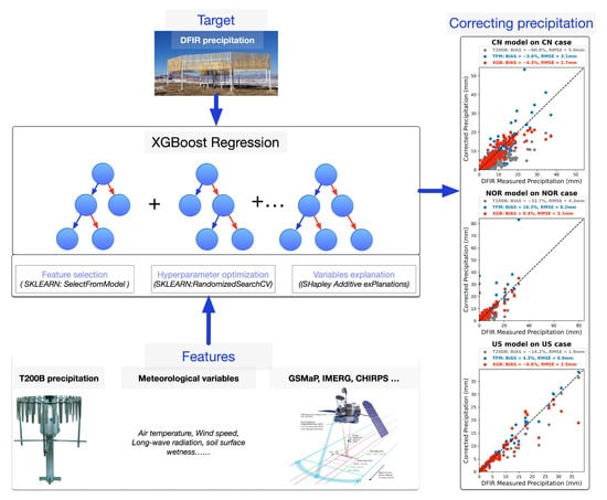
Figure 2.
The methodology of the XGBoost regression-based precipitation correction. The features include the T200 precipitation, remote sensing precipitation, and other meteorological variables. The target is the DFIR precipitation. After feature selection and hyperparameter optimization, the trained XGB model was used in correcting precipitations. The photo of the satellite is from the NASA GPM website (https://gpm.nasa.gov/missions/GPM, accessed on 2 March 2023).
Our study chose the XGBoost (Extreme Gradient Boosting) method as the machine learning method. XGBoost is a scalable tree-boosting system that uses a sparsity-aware algorithm and weighted quantile sketch for approximate tree learning [28]. It is an efficient algorithm for Gradient Boosting that iteratively generates multiple weak learners and adds their prediction results to obtain a final prediction with better performance. It is a tree-based model that uses the sum of the predictions of each tree for a given sample as the final prediction. The algorithm keeps adding trees and splitting features to grow a tree, and each time a tree is added, it learns a new function to fit the residuals of the last prediction. The predicted value of a sample is the sum of the corresponding scores of each tree. Based on the above advantages, we think the XGBoost regression (XGB) method is suitable for correcting precipitation measurements.
We also chose the traditional transfer function model (TFM) [14], as the comparison refers to the XGB method. For a fair comparison, the XGB and TFM methods were trained or fitted with the same training data, then validated with the same validation data.
Before training the XGBoost regression model, we used the RandomizedSearchCV function in scikit-learn [29] to tune the hyperparameters used. These hyperparameters include the number of estimators, the learning rate, the minimum loss reduction, the maximum depth of a tree, the minimum sum of instance weight needed in a child, the maximum delta step, the subsample ratio of the training instances, the subsample ratio, and the regularization terms on weights.
Selecting Features and Explaining the Contribution of the Features
To increase the robustness of the XGBoost regression, we employed feature selection algorithms to identify the most relevant variables from the total of 14 meteorological variables. Specifically, we utilized the SelectFromModel transformer in the scikit-learn package, which selects variables based on their weighted relevances in the XGBoost regression model, and the SequentialFeatureSelector transformer, which adds or removes variables based on the cross-validation score.
For a given number m of variables to be selected from the total of , we used the aforementioned synthesis method to identify the variable combination, resulting in 14 variable combinations. We then compared their accuracies, assessed their reliability, and made our final choice.
Given that XGBoost regression is a tree-based machine learning model, we employed SHAP (SHapley Additive exPlanations) [30], which includes a specific package for explaining the output of tree-based machine learning models. The SHAP value method is based on cooperative game theory and is used to increase the transparency and interpretability of machine learning models. We utilized this package to illustrate the impact of each variable on the model output.
Our approach allowed us to select the most relevant variables and avoid overfitting, thereby increasing the robustness of our regression model.
2.3. The Transfer Function Method
The transfer function model (TFM) developed in [14] was chosen as the comparison reference, since it has been tested in previous studies using reliable data sources. The TFM method is,
where is the catch efficiency which can be obtained by Equation (2) using the DFIR and T200B observation. [mm] is the observed precipitation to be corrected, such as the T200B observation. [mm] is the corrected precipitation or the DFIR observation. a, b, and c are coefficients calibrated using the observed wind speed (U [m/s]), air temperature (), and the observed . In this study, a, b, and c were recalibrated using our observations in Table 1. If a, b, and c were calibrated, then Equation (1) can be used to correct the T200B observation out of the training period.
2.4. Accuracy Metrics
The root-mean-square error () and the total mass bias () were used to measure the performance of the precipitation correction methods.
The and could be formulated as,
where and represent the precipitation before and after the correction at the day. n is the number of precipitation events intervals.
3. Results
3.1. How Much Precipitation Was Under-Estimated?
3.1.1. In Situ Underestimation
We compared the measured precipitation by the DFIR and T200B to clarify how much precipitation was underestimated by the T200B (Figure 3). The T200B captured 1415.6 mm of precipitation during the study period, while the DFIR captured 2855.8 mm. The annual precipitation was estimated to be about 713.9 mm/year from the DFIR and 353.9 mm/year from the T200B, considering that the study period spanned about four years. The precipitation from the T200B accounts for 49.6% of the DFIR. This means that the T200B underestimated precipitation by more than one-half. The T200B is a single-fenced instrument, and therefore, it is likely that a significant amount of precipitation was not captured.
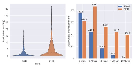
Figure 3.
Comparison between the T200B and DFIR observations of precipitation. The (left) is the frequency distribution of the two types of observations. The (right) is the segmented statistical precipitation for the two types of observations.
We analyzed the frequency distribution of precipitation from the T200B and the DFIR in daily intervals. The mean precipitation for the T200B was 2.4 mm/day, with a standard deviation of 2.8 mm/day. For the DFIR, the corresponding values were 4.8 mm/day and 5.8 mm/day. The maximum precipitation captured by the T200B was 19.5 mm/day, while the DFIR captured a maximum of 37.1 mm/day, much larger than that of the T200B.
The segmented statistics in 5 mm intervals showed that the T200B captured less precipitation in almost all ranges. In small precipitation events (0–5 mm/day), the T200B captured 20.9% more precipitation than the DFIR. However, the T200B captured less precipitation in the other ranges than the DFIR. The underestimation percentage was 49.1% for 5–10 mm/day events, increasing to 68.4% for 10–15 mm/day events, 87.5% for 15–20 mm/day events, and 100% for precipitation greater than 20 mm/day. These results indicate that the T200B has a limited capacity to capture heavy precipitation events. The heavier the precipitation, the more the T200B missed. It should be noted that this does not mean the T200B cannot capture heavy precipitation but rather that it underestimated heavy precipitation events to a greater degree.
We separately analyzed the possible missing precipitation captured by the DFIR and T200B. During the approximately four years, the DFIR was found to have missed approximately 9.5 mm of precipitation measured by the T200B, while the T200B missed approximately 127.8 mm of precipitation that the DFIR measured. The results suggest that the DFIR can detect more precipitation than the T200B. We also found that neither the T200B nor the DFIR can effectively observe small precipitation events, particularly those less than 1 mm/day. Over the four years, both the T200B and the DFIR missed approximately 600 small precipitation events (<1 mm/day) each.
3.1.2. Misestimation of Precipitation by Remotely Sensed Precipitation
We compared the remotely sensed precipitation to clarify how much precipitation was underestimated by the IMERG, GSMaP, and CHIRPS (Figure 4). The IMERG, GSMaP, and CHIRPS datasets all underestimated precipitation compared to the DFIR observations. The IMERG estimated a total of 1585.7 mm for the entire study period and had the most underestimation at 44.5%, while the CHIRPS estimated a total of 2822.6 mm and had the least underestimation at 1.2%. On the deviation error, the GSMaP had the least RMSE of 4.2 mm/day, while the CHIRPS had an RMSE of 9.2 mm/day. All three datasets had large deviations from the truth, but relatively speaking, the IMERG and GSMaP datasets were closer to the DFIR observations, while the CHIRPS had a very large bias, even up to 140 mm/day.
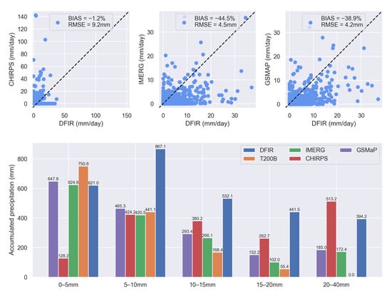
Figure 4.
The comparison among remotely sensed precipitations and in situ DFIR observations. The upper subfigures are the scatter plots between the DFIR and the remotely sensed precipitations (CHIRPS, IMERG, and GSMaP). The lower bar graph compares precipitation datasets in different daily precipitation ranges from 0–5 mm/day to 20–40 mm/day. The precipitation values are labeled above each bar.
We investigated the performance of precipitation datasets in daily precipitation ranges from 0–5 mm/day to 20–40 mm/day. In each range, precipitation values were summed as the total precipitation for each dataset. The 0–5 mm/day range had the smallest difference between the remotely sensed datasets and the DFIR, except for the CHIRPS. In this range, the DFIR had a total value of 621.0 mm, while the GSMaP and the IMERG were 647.8 mm and 624.6 mm, respectively. The CHIRPS had a small value of 128.2 mm.
The accumulated precipitation of the GSMaP and IMERG was high in small precipitation ranges, but low in large precipitation ranges. In contrast, the CHIRPS exhibited the opposite tendency, having a substantial underestimation in smaller precipitation events, but approaching the DFIR observations at heavy precipitation events (20–40 mm). Moreover, the GSMaP and IMERG approximated T200B in smaller precipitation event ranges. For precipitation events above 10 mm/day, the remotely sensed precipitation values were relatively reasonable compared to the DFIR, whereas T200B had only a few observed events, particularly in the 20–40 mm/day range.
In short, the remotely sensed precipitation datasets underestimated precipitation to varying extents. Even so, they performed better than the T200B observation in high precipitation events, especially in the 20–40 mm/day range. It indicates that remotely sensed precipitation is seldom influenced by wind, which is a major factor influencing in situ precipitation measurements.
3.2. How Can the Machine Learning Method Promote the Bias Correction of Single Fenced Precipitation Measurements?
3.2.1. Feature Selection
Firstly, we used all variables observed at the Yakou station (Figure 5). All meteorological variables were used as the training set, and the DFIR data were used as the true values. The XGBoost regression algorithm was used for training. The training results showed that the and were 0.93 and 0.73 mm, respectively. The and were 0.83 and 1.36 mm in the validation period, respectively.
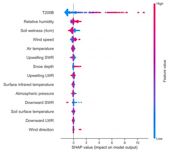
Figure 5.
The SHAP values of all meteorological variables. Each line in the graph represents a feature; the horizontal coordinates are SHAP values. A dot represents a sample. The redder the color, the larger the value of the feature itself. The bluer the color, the smaller the value of the feature itself.
We utilized SHAP values to evaluate the contribution or importance of each meteorological variable to the model’s prediction. The SHAP values provide an indication of how much the corrected precipitation is likely to change with the alteration of each feature. The results present a preliminary view of the importance of each variable in achieving the best score when all variables were employed. Figure 5 depicts the importance of all meteorological variables. Among them, the precipitation from the T200B observations is deemed the most influential, followed by relative humidity, soil surface wetness, wind speed, and air temperature. In this case, the T200B values have the broadest SHAP value ranging from −1 to about 11, signifying their significant influence on the corrected results. The larger the T200B precipitation observation, the greater the corrected precipitation. Notably, the variable importance would change if the composition of the variables were altered, such as if some were removed or added.
We utilized various feature selection algorithms, including the SELECTMODEL, to pinpoint the most significant meteorological variables for precipitation correction. By doing so, we avoided overfitting the machine-learning-based precipitation correction model. Our results demonstrated that selecting too few or too many variables did not enhance the accuracy of the precipitation correction model. Instead, a U-shaped trend in the accuracy (as measured by the RMSE) of precipitation correction was observed as the number of variables increased, highlighting the significance of selecting variables with stronger correlation to enable more precise precipitation correction learning (Figure 6).
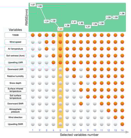
Figure 6.
The change of according to different variable combinations in the XGB regression method. There are 14 columns in which the selected variables are marked orange. The number of selected variables increased from 1 to 14 along the X-axis. The corresponding is noted at the top of each column.
After several selection iterations, T200B precipitation, air temperature, wind speed, surface soil moisture, and upward longwave radiation were identified as the primary correlations to be calibrated. The resulting SHAP values suggest that, in addition to the T200B variable, air temperature, wind speed, soil surface wetness, and upwelling longwave radiation have the widest range of effects on corrected results (Figure 7). Wind speed had a positive relationship with the magnitude of the correction for precipitation, while lower air temperature corresponded to higher corrected precipitation. Surprisingly, smaller soil moisture led to larger corrected precipitation.

Figure 7.
The SHAP value of the selected five variables. Each line in the graph represents a feature, and the horizontal coordinates are SHAP values. A dot represents a sample. The redder the color, the larger the value of the feature itself. The bluer the color, the smaller the value of the feature itself.
The use of these five variables resulted in the most accurate correction. During the training period, the and were 0.91 and 0.81 mm, respectively. During the validation period, the and were 0.86 and 1.24 mm, respectively. This result was superior to using the full set of meteorological variables for machine learning, indicating that only a few key meteorological variables are necessary to better recover precipitation values from T200B observations to close to the true value.
3.2.2. Corrected Precipitation Results Using In Situ Meteorological Variables
We utilized two methods, XGB and TFM, to correct the T200B precipitation observation. The XGB employed the five features selected in Section 3.2.1 for training and prediction, while the TFM solely used air temperature and wind speed, as required by the method.
Our results demonstrate that the XGB method outperforms the TFM method in all cases (Figure 8). It achieved the best BIAS accuracies of −2.7%, −5.0%, and −7.0% for 1 h, 6 h, and 1 day intervals, respectively, while the TFM had corresponding accuracies of −27.6%, −8.5%, and −13.3%. Compared to the significant underestimation of the T200B observation (with approximately 50% underestimated), both the XGB and TFM methods showed considerable improvement in the BIAS measure. The XGB method had the least BIAS.
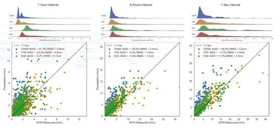
Figure 8.
The corrected precipitation results are presented in three separate columns for 1 h, 6 h, and 1 d intervals. Each column represents the total precipitation during the respective time step. The XGBoost-corrected results (XGB), traditional transfer function method-corrected results (TFM), and the uncorrected T200B observation (Y-axis) are compared with the DFIR observation (X-axis). The comparisons include scatter plots and frequency distributions. A distinct color represents each correction method. For example, the XGBoost method is in green. The accuracy of each method is listed in the scatter plots. Only data from the validation period are used here.
Regarding RMSE, the XGB method outperformed the T200B observation, particularly in the 6 h interval case, where XGB achieved an RMSE of 1.2 mm, half that of the T200B observation.
Both the XGB and TFM methods significantly improved the frequency distribution of corrected precipitation. The original T200B precipitation distribution was concentrated in the lower values on all time scales, which differs from the DFIR precipitation distribution. After correction, the T200B precipitation in the low-value interval was suppressed, and precipitation in the high-value interval was increased. The corrected precipitation of the XGB and TFM methods was closer to the DFIR precipitation in the frequency distribution.
The frequency distributions of corrected precipitation of the XGB and TFM methods differed. On the 1 h interval, the frequency distribution of precipitation obtained by the XGB correction method was closer to the DFIR precipitation. The TFM method corrected the original T200B precipitation, but many corrected precipitation values were still clustered in the low-value range. On the 6 h interval, the frequency distribution of corrected precipitation for both the XGB and TFM methods was closer to that of the DFIR precipitation. The XGB precipitation correction agreed better with the DFIR of both low and high values of precipitation, while the TFM precipitation tended to be underestimated in the high-value interval. This was evident from the scatterplot, where the TFM precipitation was largely biased below the 1:1 line in the high-value interval on the 6 h case (Figure 8). In the 1-day case, a similar problem existed: the TFM-corrected precipitation was prone to underestimating the actual precipitation in the high-value interval.
3.3. How Could Remotely Sensed Precipitation Be Used in Machine Learning to Promote Precipitation Correction?
We integrated remotely sensed precipitation data into the XGB regression method to improve precipitation correction (Figure 9). We compared three datasets: (1) the corrected precipitation from the XGB method with the remotely sensed data, (2) the corrected precipitation from the traditional TFM method, and (3) the uncorrected T200B data. To ensure consistency, we selected daily remotely sensed data and analyzed our results daily. We also divided the study period into two halves, using the first half for training and the second half for validation.
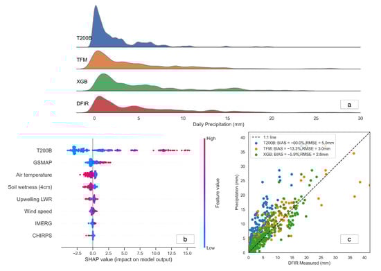
Figure 9.
The corrected precipitation results by integrating the remotely sensed precipitation (GSMAP, IMERG, and CHIRPS). (a) The frequency distributions of precipitation datasets using the XGB and TFM methods of the T200B and the DFIR. (b) The importance of explanation using SHAP values. Each line in the graph represents a feature; the horizontal coordinates are SHAP values. A dot represents a sample. The redder the color, the larger the value of the feature itself. The bluer the color, the smaller the value of the feature itself. (c) The comparison between the corrected precipitation and the truth value using the DFIR observation. The accuracies (BIAS and RMSE) are listed in the upper left.
Our results demonstrate a marginal improvement in the accuracy of the XGB regression method, including the BIAS and RMSE, following the incorporation of remotely sensed precipitation data into the machine-learning regression. Specifically, the BIAS and RMSE of the XGB method utilizing remotely sensed data were −5.9% and 2.8 mm, respectively, while the accuracy of the XGB method sans remotely sensed data was −7.0% and 2.9 mm, respectively. Furthermore, the frequency distribution of precipitation data corrected by integrating remotely sensed data was much closer to the actual precipitation of the DFIR.
We also utilized SHAP values to analyze the contribution of remotely sensed data in the XGB regression model. Our results indicate that the T200B data remain the most influential variable in the final corrected results. However, the GSMaP product in the remotely sensed precipitation data ranks second in importance, playing a more significant role than other variables, including ground-based observations and other remote sensing products. This suggests that the GSMaP data replace part of the influence that arises from the role of in situ wind speed on precipitation correction. The SHAP plot indicates that the greater the precipitation measured by GSMaP, the greater its corresponding corrected precipitation value. Moreover, the precipitation observation of GSMaP is in good agreement with the actual precipitation, as shown in Figure 4. The other two types of remotely sensed precipitation products, IMERG and CHIRPS, have limited influence on precipitation correction, and their SHAP values are restricted to a very narrow interval.
Our findings suggest that the remotely sensed GSMaP data are more valuable for precipitation correction in this high-altitude region than the air temperature and wind speed observations.
4. Discussion
4.1. Can the Machine Learning Method Be Transferred to Other Regions?
One of our biggest concerns is the transferability of the XGB correction method from one site to another with completely different environmental conditions. To address this issue, we compared the performance of the XGB method at the Yakou site in China (CN) with that of stations in Norway (NOR) and the United States (US), using data from [14] (Figure 10). We trained the XGB model on one site and then applied the trained model to another site. For example, we trained the XGB model on the CN station, and then the trained model was used to correct the single-fence T200B precipitation in the NOR station only using the data from the NOR station.
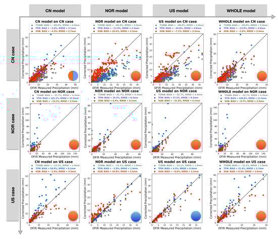
Figure 10.
The transferring performance of the XGB precipitation correction method between different sites in Norway (NOR), the United States (US), and our study area in China (CN). The X-axis represents the trained model in CN, NOR, and US, while the Y-axis represents the site cases in CN, NOR, and US. Each subfigure displays the result of the trained model applied to a specific site. For example, ’CN model on US case’ indicates that the trained CN model using CN data was applied to correct the US case. The WHOLE model was trained using the training data from NOR, US, and CN. The XGB results (in red) are the uncorrected T200B or single-alter gauge observation (in grey) and the traditional TFM correction (in blue) are scattered. The BIAS and RMSE are listed in each subfigure. A solid cycle located in the lower-right of each subfigure indicates if the XGB model outperforms the TFM model, with orange meaning the XGB model outperforms the TFM model in RMSE and BIAS, and blue meaning the opposite. Half blue and half orange indicate that the XGB model outperforms the TFM model in one of the RMSE and BIAS metrics.
In this study, we also compared the performance of the XGB method with that of the TFM method in various scenarios. The TFM method was developed to correct wind-induced undercatch of precipitation, particularly snowfall. The TFM method only uses wind speed and air temperature as inputs and has demonstrated good agreement at both the Norway (NOR) and the United States (US) stations [14].
In our comparison, we utilized five features: wind speed, air temperature, two remotely sensed precipitation datasets (the GSMaP and IMERG), and the uncorrected single-alter precipitation observation (T200B). We used DFIR observations from three sites as the truth precipitation for XGB training or the regression of the TFM method. The wind speed, air temperature, and single-alter precipitation observation were obtained from the US, NOR, and CN stations, respectively. The datasets were divided into two halves of equal length in chronological order, with the first half being the training dataset and the second half being the evaluation dataset. Notably, for a fair comparison, we calibrated the parameters for XGB and TFM using the same training dataset and evaluated them on the same target dataset. The parameters of the TFM method reported in [14] were not used in this study.
We first examined the performance of the XGB and TFM models in correcting local precipitation in three separate sites using only local data for training and validation. Results showed that both methods effectively corrected the underestimation of single-fence precipitation measurements in the NOR, US, and CN sites. The underestimation ranged from 60.0 to 14.2%, but after correction, the BIAS decreased to a range between 0.4% and 6.6%. The XGB method outperformed the TFM method in the NOR site regarding RMSE and BIAS, while the TFM method outperformed the XGB method in the US site. In the CN site, the RMSE of the XGB method was better than the TFM, but the TFM had a better BIAS. Overall, both methods effectively corrected local precipitation in the three sites.
Next, we examined the transferability of the XGB and TFM methods across the three sites. This involved training a model using local data and using the trained model to correct precipitation in another site. It means there are six cross-examinations. The results showed that the XGB method had better transferability than the TFM method. In the cross-examinations (Figure 10), the XGB model outperformed the TFM method in five out of six cases, such as the ‘CN model on US case’. For example, in the ‘CN model on US case’, the XGB model was trained using data from the CN site and then used to correct single-fence precipitation data in the US site. This correction reduced the BIAS from −14.4% to −5.6%, while the TFM method did not correct the underestimation. This illustrates the superior transferability of the XGB method. These findings suggest that reasonable precipitation corrections can be made at a site without corresponding DFIR precipitation data using a trained machine-learning model from another location.
Our results also suggest that the introduction of remote sensing data greatly enhances the migration capability of the XGB machine learning model across different sites with varying environmental conditions. In Figure 10, the XGB model was trained using all the training data from the three sites (named as WHOLE model) and was then used to separately correct the single-fence precipitation in each of the three sites. In two out of three sites, the XGB correction model outperformed other model sets, including the local model set, such as the ‘CN model on CN case’. This implies that introducing more data can improve the capacity of the machine-learning model. However, this is not the case for the TFM model, where all three site tests indicated that introducing more data brings more errors for the TFM.
We evaluated the machine learning model’s ability to transfer between the Yakou (CN) site and the Norway and United States sites. Our results show that machine learning methods incorporating remote sensing data have better transferability than traditional methods. This improved transferability may be attributed to two factors. The first is the better generalization ability of machine learning, particularly the XGBoost method [28], which can eliminate outliers and achieve better learning results. The second factor is the use of remotely sensed precipitation data. In this study, we introduced remotely sensed precipitation data GSMaP [21] and IMERG [22]. Satellite data are less likely to be affected by ground conditions than ground-based meteorological data. For example, ground-based precipitation observations can be influenced by wind speeds [31], whereas satellite data are not affected by wind speed. Satellite data have a significant advantage in precipitation observations for high wind speeds, as our study shows. As more and better remote sensing precipitation data become available, it could be expected to obtain better machine learning-corrected precipitation results.
4.2. Advantages and Notices of Applying Machine Learning Method in Correcting Precipitation Measurement
We found that increasing the number of variables did not necessarily lead to better training results. On the contrary, removing irrelevant variables led to better results, making the trained model more robust. Our machine-learning model was optimal with five variables, and the RMSE for the validation period was 1.24 mm. However, after adding variables such as downward longwave radiation, the model’s accuracy was not improved, and it was 1.28 mm. Although the change in accuracy due to the addition of variables was relatively small, it illustrated that adding variables of low importance or relevance did not improve the accuracy of the learning model.
The XGBoost feature selection algorithm could automatically identify the critical variables according to their importance, such as air temperature, wind speed, surface soil moisture, and upward longwave radiation. In traditional calibration methods, wind speed and air temperature were usually substituted as the main variables for calculating various precipitation losses [4]. In addition to essential variables such as wind speed, the feature selection method identified upward longwave radiation, a radiation-related meteorological element, as a critical factor in precipitation correction, which had been neglected in previous correction methods. Our SHAP variable contribution plots showed that upward longwave radiation and soil surface moisture contributed significantly to the precipitation correction results (Figure 7). We believe that longwave radiation, closely associated with radiative energy transfer, affects precipitation capture rate. Therefore, precipitation occurrence is likely to significantly relate to surface longwave radiation. A similar study also reported the influence of blowing snow or snowfall on long wave radiation [32], but this finding has not been introduced into the precipitation correction. These findings suggest that the machine learning algorithm can uncover the hidden longwave radiation as an essential influence factor, which is a variable often ignored in previous empirical algorithms. In this case, the feature selection method of machine learning suggests an excitingly different approach from the traditional correction methods.
It should be noted that scale difference exists between remotely sensed precipitation products and in-situ meteorological observations. The GSMaP and IMERG have a resolution of , about a 10 km resolution grid. The CHIRPS have a finer resolution of . The three RS precipitation datasets have a wider cover than the point-scale precipitation measurements, leading to a spatial scale issue. It is possible that higher resolution remotely sensed precipitation data would better contribute to the precipitation correction. For example, some studies have used ground radar to bridge the scale gaps between precipitation gauge and satellite [33]. The spatial representativeness of the in situ instruments, such as the T200B and DFIR, should also be considered in the future comparison.
4.3. Implications of Machine-Learning Method on Obtaining More Accurate Precipitation in the High Altitude Region in the Future
We tested a machine learning method for correcting precipitation measurements that differ from traditional statistical models. This method performed better than traditional models at the high-altitude site. This method used more meteorological variables than traditional methods, such as long-wave radiation and surface soil moisture. Traditional statistical models only use air temperature and wind speed as inputs [10], mainly considering the transferability of the method: as many regions historically did not have other observations besides air temperature and wind speed. Given that those meteorological variables deployed in high-altitude areas are becoming increasingly abundant [26], it is hopeful to include more meteorological variables in the future correction of precipitation measurement, promoting machine learning and traditional statistical models.
The addition of remote sensing precipitation data can promote the transferability of precipitation correction methods based on machine learning. Although ground observation meteorological variables such as air temperature and precipitation are still needed, with the improvement of remote sensing observation capabilities, machine learning is expected to use only remote sensing precipitation to obtain ground precipitation “truth”. This depends on three aspects: (1) Richer remote sensing data. The current trend of remote sensing precipitation products has integrated multi-source platform precipitation [34]. More ‘big’ remote sensing data is expected to be included with the launch of more satellite precipitation observations (such as FengYun-4A [35]). (2) More advanced machine learning methods. For example, some work has used different deep-learning methods to correct precipitation occurrence and intensity separately [36]. Some of the latest developments, such as in Long Short-Term Memory (LSTM) [37] and transformer methods [38], are expected to be applied to the correction of precipitation measurement. (3) More comprehensive model verification. In addition to site verification, verifying the hydrological effects of precipitation correction with watershed-scale hydrological models can more accurately evaluate the hydrological effects of precipitation correction [39].
Our work is based on the premise that DFIR equipment is used as the “actual” precipitation. However, the maintenance cost of establishing a DFIR device in the current high-altitude environment would be huge. Because such equipment still requires manual maintenance, it is also unimaginable to widely establish such equipment in high-altitude areas. Therefore, it is necessary to establish a small number of DFIRs in key areas. Our observations show that the T200B precipitation at high altitudes can underestimate DFIR precipitation by more than 50%, which far exceeds the observed precipitation in other regions [40]. However, in the Tibetan Plateau region spanning multiple meteorological zones [41], DFIR precipitation is rare, illustrating the necessity of deploying DFIR in high-altitude areas. If there is no such device as DFIR to provide actual precipitation, the widely used reanalysis precipitation data and remote sensing precipitation data can only be validated using sparse, uncorrected precipitation data, which will inevitably bring misunderstandings of hydrological processes.
5. Conclusions
In contrast to the traditional TFM method, we utilized a machine-learning approach (XGBoost) to correct precipitation measurements at high altitudes. This method incorporated both meteorological variables and remote sensing precipitation data. We also investigated the transferability of the XGBoost regression method across the Yakou site and other sites in Norway and the United States.
Our findings revealed that the T200B instrument inadequately captured precipitation at high altitudes. Specifically, the underestimation of precipitation reached 51.4% of DFIR measurements, notably higher than similar measurements in the Arctic or lower altitudes. Furthermore, we observed that both the T200B and DFIR methods failed to effectively capture small precipitation events, particularly those less than 1 mm/day. Notably, remote sensing precipitation datasets, including CHIRPS, IMERG, and GSMaP, consistently underestimated precipitation when compared to DFIR observations. While IMERG and GSMaP datasets were closer to DFIR observations, the CHIRPS dataset exhibited significant bias. Despite this, remote sensing data performed better than T200B observations during high precipitation events, and we found that remotely sensed precipitation was rarely influenced by wind, a major factor that influences in situ precipitation measurements.
The XGBoost method demonstrated superior performance in correcting precipitation measurements at high altitudes. Specifically, the XGBoost method improved the bias at the Yakou site from −61.3 to −2.7% at a 1 h interval, whereas the traditional TFM method improved the bias from −61.3 to −27.6%. Both the XGBoost and TFM methods exhibited considerable improvement in the BIAS measure and the frequency distribution of corrected precipitation. However, the XGBoost precipitation correction agreed better with the DFIR for both low and high precipitation values, while the TFM precipitation tended to be underestimated in the high-value interval. After incorporating remotely sensed precipitation data into the XGBoost method, the BIAS and RMSE slightly improved. Though only a slight improvement, remote sensing data, specifically GSMaP precipitation, ranked second in importance and replaced part of the influence of in situ wind speed on precipitation correction. Consequently, our results suggest a potential opportunity to use remote sensing data rather than in situ meteorological observations to correct precipitation, indicating a more straightforward and widespread use.
Our findings suggest that the machine learning method excels at identifying crucial prospective variables related to bias correction. In addition to air temperature and wind speed, which are conventionally utilized for correcting precipitation, the machine learning method automatically selected soil surface moisture, upwelling longwave radiation, and remote sensing data (specifically GSMaP) to achieve optimal corrected outcomes.
We also investigated the transferability of the XGBoost method among the NOR, US, and CN sites. Results indicate that the XGBoost method had superior transferability over the TFM method. Specifically, the XGBoost model outperformed the TFM method in five out of six cases when the trained XGBoost model was cross-validated among different sites. This suggests that reasonable precipitation corrections can be made at a site without corresponding DFIR precipitation data using a trained machine-learning model from another location. Additionally, our results suggest that the introduction of remote sensing data enhances the migration capability of the XGBoost machine learning model across different sites with varying environmental conditions. Its enhanced transferability is a result of two factors: enhanced generalization capability of machine learning and utilization of remotely sensed precipitation data. Given that satellite data have a significant advantage in precipitation observations for high wind speeds, we anticipate that as more and better remote sensing precipitation data become available, machine learning-corrected precipitation outcomes will continue to be improved.
Our research highlights the potential of combining advanced machine learning techniques with richer remote sensing data as a promising future strategy for achieving more accurate precipitation predictions in high-altitude regions.
Author Contributions
Conceptualization, H.L. (Hongyi Li); methodology, H.L. (Hongyi Li); coding, H.L. (Hongyi Li); validation, H.L. (Hongyi Li).; writing—original draft preparation, H.L. (Hongyi Li); writing—review and editing, H.L. (Hongyi Li), H.L. (Huajin Lei), Y.Z., X.H.; visualization, H.L. (Hongyi Li); supervision, H.L. (Hongyi Li); Data, H.L. (Hongyi Li), Y.Z., H.L. (Huajin Lei), X.H. All authors have read and agreed to the published version of the manuscript.
Funding
This research was funded by the Joint Funds of the National Natural Science Foundation of China (U22A20564) and the National Natural Science Foundation of China (Grant numbers: 41971325).
Data Availability Statement
The data presented in this study are available on request from the corresponding author. The data are not publicly available due to the data sharing policy.
Conflicts of Interest
The authors declare no conflict of interest.
Abbreviations
The following abbreviations are used in this manuscript:
| BIAS | total mass BIAS |
| CCCASON | Climate Change Canada Automated Surface Observation Network |
| CHIRPS | Climate Hazards Group InfraRed Precipitation with Station data |
| CMORPH | CPC MORPHing technique |
| CN station | Yakou station in ChiNa |
| DFIR | Double Fence Intercomparison Reference |
| GSMaP | Global Satellite Mapping of Precipitation |
| IMERG | Integrated Multi-satellitE Retrievals for GPM |
| NOR station | the used station in NORway |
| RMSE | Root-Mean-Square Error |
| SHAP | SHapley Additive exPlanations |
| TFM | Transfer Function Method |
| TRMM | Tropical Rainfall Measuring Mission |
| US station | the used station in United States |
| WMO | World Meteorological Organization |
| WMO-SPICE | WMO - Solid Precipitation Intercomparison Experiment |
| XGBoost | Extreme Gradient Boosting |
| XGB | XGBoost regression method |
References
- Ma, J.; Li, H.; Wang, J.; Hao, X.; Shao, D.; Lei, H. Reducing the Statistical Distribution Error in Gridded Precipitation Data for the Tibetan Plateau. J. Hydrometeorol. 2020, 21, 2641–2654. [Google Scholar] [CrossRef]
- Yang, D.; Goodison, B.E.; Metcalfe, J.R.; Louie, P.; Leavesley, G.; Emerson, D.; Hanson, C.L.; Golubev, V.S.; Elomaa, E.; Gunther, T.; et al. Quantification of Precipitation Measurement Discontinuity Induced by Wind Shields on National Gauges. Water Resour. Res. 1999, 35, 491–508. [Google Scholar] [CrossRef]
- Chen, R.; Liu, J.; Kang, E.; Yang, Y.; Han, C.; Liu, Z.; Song, Y.; Qing, W.; Zhu, P. Precipitation Measurement Intercomparison in the Qilian Mountains, North-Eastern Tibetan Plateau. Cryosphere 2015, 9, 1995–2008. [Google Scholar] [CrossRef]
- Sugiura, K.; Ohata, T.; Yang, D. Catch Characteristics of Precipitation Gauges in High-Latitude Regions with High Winds. J. Hydrometeorol. 2006, 7, 984–994. [Google Scholar] [CrossRef]
- Jia, Y.; Li, Z.; Wang, F.; Chen, P. Correction of Precipitation Measurement for Weighing Precipitation Gauges in a Glacierized Basin in the Tianshan Mountains. Front. Earth Sci. 2023, 11, 1115299. [Google Scholar] [CrossRef]
- Yang, D. Double Fence Intercomparison Reference (DFIR) vs. Bush Gauge for “True” Snowfall Measurement. J. Hydrol. 2014, 509, 94–100. [Google Scholar] [CrossRef]
- Goodison, B.E.; Louie, P.Y.T.; Yang, D. WMO Solid Precipitation Measurement Intercomparison–Final Report; Technical Report WMO/TD—No. 872; World Meteorological Organization: Geneva, Switzerland, 1998. [Google Scholar]
- Yang, D.; Ohata, T. A Bias-Corrected Siberian Regional Precipitation Climatology. J. Hydrometeorol. 2001, 2, 122–139. [Google Scholar] [CrossRef]
- Yang, D. An Improved Precipitation Climatology for the Arctic Ocean. Geophys. Res. Lett. 1999, 26, 1625–1628. [Google Scholar] [CrossRef]
- Yang, D.; Kane, D.; Zhang, Z.; Legates, D.; Goodison, B. Bias Corrections of Long-Term (1973–2004) Daily Precipitation Data over the Northern Regions. Geophys. Res. Lett. 2005, 32, L19501. [Google Scholar] [CrossRef]
- Pan, X.; Yang, D.; Li, Y.; Barr, A.; Helgason, W.; Hayashi, M.; Marsh, P.; Pomeroy, J.; Janowicz, R.J. Bias Corrections of Precipitation Measurements across Experimental Sites in Different Ecoclimatic Regions of Western Canada. Cryosphere 2016, 10, 2347–2360. [Google Scholar] [CrossRef]
- WMO. IOM Report, 131. WMO Solid Precipitation Intercomparison Experiment (SPICE) (2012–2015); WMO: Geneva, Switzerland, 2018. [Google Scholar]
- Wolff, M.A.; Isaksen, K.; Petersen-Øverleir, A.; Ødemark, K.; Reitan, T.; Brækkan, R. Derivation of a New Continuous Adjustment Function for Correcting Wind-Induced Loss of Solid Precipitation: Results of a Norwegian Field Study. Hydrol. Earth Syst. Sci. 2015, 19, 951–967. [Google Scholar] [CrossRef]
- Kochendorfer, J.; Rasmussen, R.; Wolff, M.; Baker, B.; Hall, M.E.; Meyers, T.; Landolt, S.; Jachcik, A.; Isaksen, K.; Brækkan, R.; et al. The Quantification and Correction of Wind-Induced Precipitation Measurement Errors. Hydrol. Earth Syst. Sci. 2017, 21, 1973–1989. [Google Scholar] [CrossRef]
- Kochendorfer, J.; Nitu, R.; Wolff, M.; Mekis, E.; Rasmussen, R.; Baker, B.; Earle, M.E.; Reverdin, A.; Wong, K.; Smith, C.D.; et al. Testing and Development of Transfer Functions for Weighing Precipitation Gauges in WMO-SPICE. Hydrol. Earth Syst. Sci. 2018, 22, 1437–1452. [Google Scholar] [CrossRef]
- Smith, C.D.; Mekis, E.; Hartwell, M.; Ross, A. The Hourly Wind-Bias-Adjusted Precipitation Data Set from the Environment and Climate Change Canada Automated Surface Observation Network (2001–2019). Earth Syst. Sci. Data 2022, 14, 5253–5265. [Google Scholar] [CrossRef]
- Zhao, Y.; Chen, R.; Han, C.; Wang, L.; Guo, S.; Liu, J. Correcting Precipitation Measurements Made with Geonor T-200B Weighing Gauges near the August-One Ice Cap in the Qilian Mountains, Northwest China. J. Hydrometeorol. 2021, 22, 1973–1985. [Google Scholar] [CrossRef]
- Smith, C.D.; Ross, A.; Kochendorfer, J.; Earle, M.E.; Wolff, M.; Buisán, S.; Roulet, Y.A.; Laine, T. Evaluation of the WMO Solid Precipitation Intercomparison Experiment (SPICE) Transfer Functions for Adjusting the Wind Bias in Solid Precipitation Measurements. Hydrol. Earth Syst. Sci. 2020, 24, 4025–4043. [Google Scholar] [CrossRef]
- Liu, Z.; Ostrenga, D.; Teng, W.; Kempler, S. Tropical Rainfall Measuring Mission (TRMM) Precipitation Data and Services for Research and Applications. Bull. Am. Meteorol. Soc. 2012, 93, 1317–1325. [Google Scholar] [CrossRef]
- Joyce, R.J.; Janowiak, J.E.; Arkin, P.A.; Xie, P. CMORPH: A Method That Produces Global Precipitation Estimates from Passive Microwave and Infrared Data at High Spatial and Temporal Resolution. J. Hydrometeorol. 2004, 5, 487–503. [Google Scholar] [CrossRef]
- Kubota, T.; Aonashi, K.; Ushio, T.; Shige, S.; Takayabu, Y.N.; Kachi, M.; Arai, Y.; Tashima, T.; Masaki, T.; Kawamoto, N.; et al. Global Satellite Mapping of Precipitation (GSMaP) Products in the GPM Era. In Satellite Precipitation Measurement: Volume 1; Levizzani, V., Kidd, C., Kirschbaum, D.B., Kummerow, C.D., Nakamura, K., Turk, F.J., Eds.; Advances in Global Change Research; Springer International Publishing: Cham, Switzerland, 2020; pp. 355–373. [Google Scholar] [CrossRef]
- Huffman, G.J.; Bolvin, D.T.; Braithwaite, D.; Hsu, K.L.; Joyce, R.J.; Kidd, C.; Nelkin, E.J.; Sorooshian, S.; Stocker, E.F.; Tan, J.; et al. Integrated Multi-satellite Retrievals for the Global Precipitation Measurement (GPM) Mission (IMERG). In Satellite Precipitation Measurement: Volume 1; Levizzani, V., Kidd, C., Kirschbaum, D.B., Kummerow, C.D., Nakamura, K., Turk, F.J., Eds.; Advances in Global Change Research; Springer International Publishing: Cham, Switzerland, 2020; pp. 343–353. [Google Scholar] [CrossRef]
- Gagne, D.J.; McGovern, A.; Xue, M. Machine Learning Enhancement of Storm-Scale Ensemble Probabilistic Quantitative Precipitation Forecasts. Weather Forecast. 2014, 29, 1024–1043. [Google Scholar] [CrossRef]
- Wang, F.; Tian, D.; Carroll, M. Customized Deep Learning for Precipitation Bias Correction and Downscaling. Geosci. Model Dev. 2023, 16, 535–556. [Google Scholar] [CrossRef]
- Li, H.; Li, X.; Yang, D.; Wang, J.; Gao, B.; Pan, X.; Zhang, Y.; Hao, X. Tracing Snowmelt Paths in an Integrated Hydrological Model for Understanding Seasonal Snowmelt Contribution at Basin Scale. J. Geophys. Res. Atmos. 2019, 124, 8874–8895. [Google Scholar] [CrossRef]
- Che, T.; Li, X.; Liu, S.; Li, H.; Xu, Z.; Tan, J.; Zhang, Y.; Ren, Z.; Xiao, L.; Deng, J.; et al. Integrated Hydrometeorological, Snow and Frozen-Ground Observations in the Alpine Region of the Heihe River Basin, China. Earth Syst. Sci. Data 2019, 11, 1483–1499. [Google Scholar] [CrossRef]
- Funk, C.; Peterson, P.; Landsfeld, M.; Pedreros, D.; Verdin, J.; Shukla, S.; Husak, G.; Rowland, J.; Harrison, L.; Hoell, A.; et al. The Climate Hazards Infrared Precipitation with Stations—A New Environmental Record for Monitoring Extremes. Sci. Data 2015, 2, 150066. [Google Scholar] [CrossRef] [PubMed]
- Chen, T.; Guestrin, C. XGBoost: A Scalable Tree Boosting System. In KDD ’16: Proceedings of the 22nd ACM SIGKDD International Conference on Knowledge Discovery and Data Mining; Association for Computing Machinery: New York, NY, USA, 2016; pp. 785–794. [Google Scholar] [CrossRef]
- Pedregosa, F.; Varoquaux, G.; Gramfort, A.; Michel, V.; Thirion, B.; Grisel, O.; Blondel, M.; Prettenhofer, P.; Weiss, R.; Dubourg, V.; et al. Scikit-Learn: Machine Learning in Python. J. Mach. Learn. Res. 2011, 12, 2825–2830. [Google Scholar]
- Lundberg, S.M.; Erion, G.; Chen, H.; DeGrave, A.; Prutkin, J.M.; Nair, B.; Katz, R.; Himmelfarb, J.; Bansal, N.; Lee, S.I. From Local Explanations to Global Understanding with Explainable AI for Trees. Nat. Mach. Intell. 2020, 2, 56–67. [Google Scholar] [CrossRef]
- Masuda, M.; Yatagai, A.; Kamiguchi, K.; Tanaka, K. Daily Adjustment for Wind-Induced Precipitation Undercatch of Daily Gridded Precipitation in Japan. Earth Space Sci. 2019, 6, 1469–1479. [Google Scholar] [CrossRef]
- Yang, Y.; Palm, S.P.; Marshak, A.; Wu, D.L.; Yu, H.; Fu, Q. First Satellite-Detected Perturbations of Outgoing Longwave Radiation Associated with Blowing Snow Events over Antarctica. Geophys. Res. Lett. 2014, 41, 730–735. [Google Scholar] [CrossRef]
- Chandrasekar, V.; Chen, H. A Machine Learning Approach to Derive Precipitation Estimates at Global Scale Using Space Radar and Ground-Based Observations. In Proceedings of the IGARSS 2020—2020 IEEE International Geoscience and Remote Sensing Symposium, Waikoloa, HI, USA, 26 September–2 October 2020; pp. 5376–5379. [Google Scholar] [CrossRef]
- Lei, H.; Zhao, H.; Ao, T. Ground Validation and Error Decomposition for Six State-of-the-Art Satellite Precipitation Products over Mainland China. Atmos. Res. 2022, 269, 106017. [Google Scholar] [CrossRef]
- Ren, J.; Xu, G.; Zhang, W.; Leng, L.; Xiao, Y.; Wan, R.; Wang, J. Evaluation and Improvement of FY-4A AGRI Quantitative Precipitation Estimation for Summer Precipitation over Complex Topography of Western China. Remote Sens. 2021, 13, 4366. [Google Scholar] [CrossRef]
- Lei, H.; Zhao, H.; Ao, T. A Two-Step Merging Strategy for Incorporating Multi-Source Precipitation Products and Gauge Observations Using Machine Learning Classification and Regression over China. Hydrol. Earth Syst. Sci. 2022, 26, 2969–2995. [Google Scholar] [CrossRef]
- Yang, X.; Yang, S.; Tan, M.L.; Pan, H.; Zhang, H.; Wang, G.; He, R.; Wang, Z. Correcting the Bias of Daily Satellite Precipitation Estimates in Tropical Regions Using Deep Neural Network. J. Hydrol. 2022, 608, 127656. [Google Scholar] [CrossRef]
- Karozis, S.; Klampanos, I.A.; Sfetsos, A.; Vlachogiannis, D. A Deep Learning Approach for Spatial Error Correction of Numerical Seasonal Weather Prediction Simulation Data. Big Earth Data 2023, 1–20. [Google Scholar] [CrossRef]
- Lei, H.; Zhao, H.; Ao, T.; Hu, W. Quantifying the Reliability and Uncertainty of Satellite, Reanalysis, and Merged Precipitation Products in Hydrological Simulations over the Topographically Diverse Basin in Southwest China. Remote Sens. 2023, 15, 213. [Google Scholar] [CrossRef]
- Sevruk, B.; Ondrás, M.; Chvíla, B. The WMO Precipitation Measurement Intercomparisons. Atmos. Res. 2009, 92, 376–380. [Google Scholar] [CrossRef]
- Lei, H.; Li, H.; Zhao, H.; Ao, T.; Li, X. Comprehensive Evaluation of Satellite and Reanalysis Precipitation Products over the Eastern Tibetan Plateau Characterized by a High Diversity of Topographies. Atmos. Res. 2021, 259, 105661. [Google Scholar] [CrossRef]


Disclaimer/Publisher’s Note: The statements, opinions and data contained in all publications are solely those of the individual author(s) and contributor(s) and not of MDPI and/or the editor(s). MDPI and/or the editor(s) disclaim responsibility for any injury to people or property resulting from any ideas, methods, instructions or products referred to in the content. |
© 2023 by the authors. Licensee MDPI, Basel, Switzerland. This article is an open access article distributed under the terms and conditions of the Creative Commons Attribution (CC BY) license (https://creativecommons.org/licenses/by/4.0/).