

High Spatial and Temporal Soil Moisture Retrieval in Agricultural Areas Using Multi-Orbit and Vegetation Adapted Sentinel-1 SAR Time Series
 , , and
Abstract
:1. Introduction
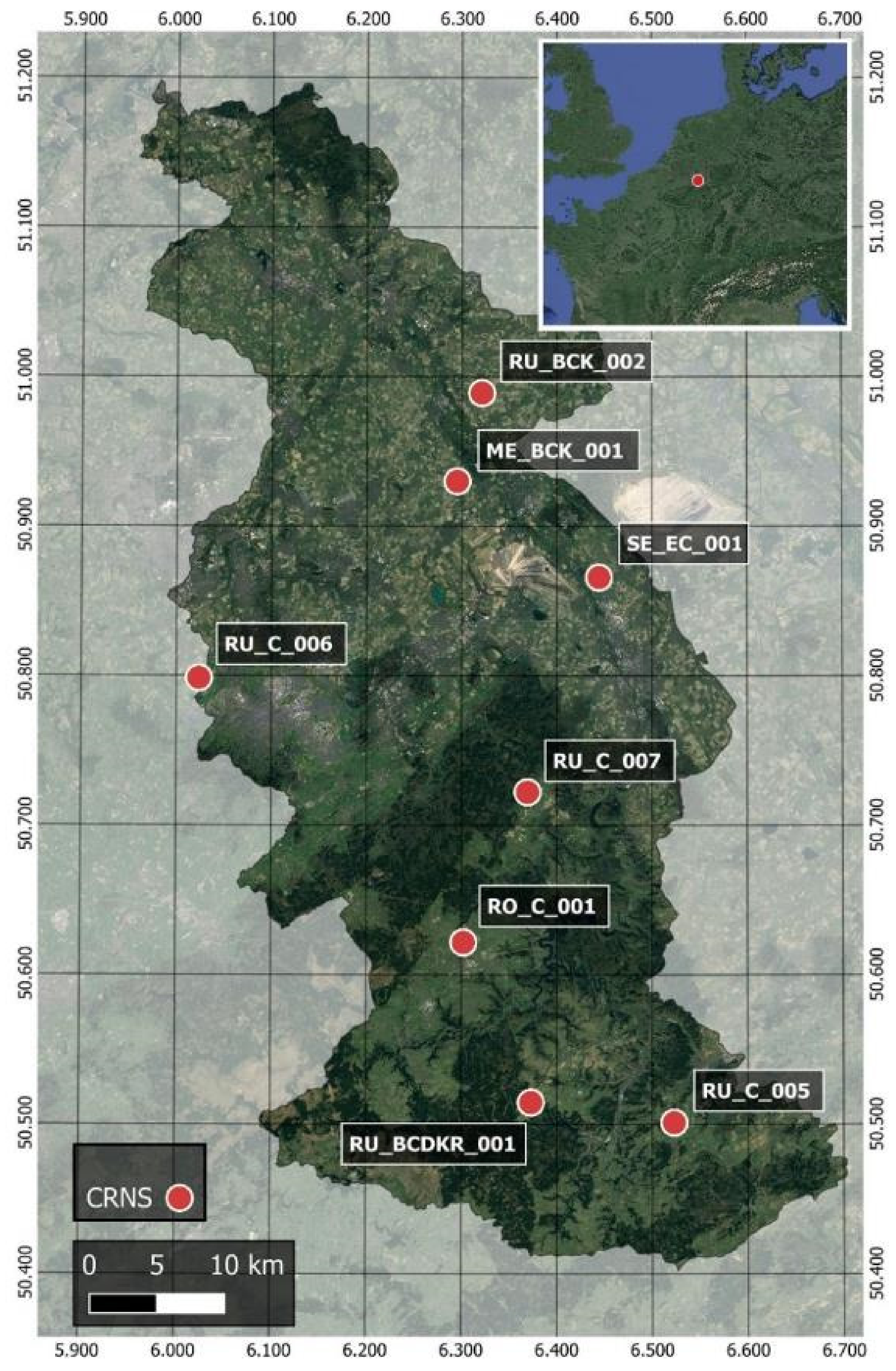
2. Study Area
3. Data
3.1. Sentinel-1 C-Band SAR
3.2. CORINE Land Cover Data
3.3. OpenLandMap Data
3.4. Global Land Data Assimilation System (GLDAS)
3.5. Cosmic-Ray Neutron Probe (CRNP) Stations
3.6. Capacitance Stations
4. Methods
4.1. Preprocessing
4.1.1. Masking
4.1.2. Spatial Filtering
4.1.3. Incidence Angle Normalization
4.1.4. Fourier Transformation
4.1.5. Vegetation Correction
4.2. Soil Moisture Estimation
4.2.1. Alpha Approximation
4.2.2. Soil Moisture to Dielectric Constant Inversion
5. Results and Discussion
5.1. Incidence Angle Normalization
5.2. Fourier Series Transformation
5.3. Vegetational Correction
5.4. Effect of Individual Processing Steps on Soil Moisture Estimation
6. Conclusions
Author Contributions
Funding
Data Availability Statement
Acknowledgments
Conflicts of Interest
References
- Velasco-Muñoz, J.F.; Aznar-Sánchez, J.A.; Batlles-delaFuente, A.; Fidelibus, M.D. Sustainable Irrigation in Agriculture: An Analysis of Global Research. Water 2019, 11, 1758. [Google Scholar] [CrossRef]
- Haddeland, I.; Heinke, J.; Biemans, H.; Eisner, S.; Flörke, M.; Hanasaki, N.; Konzmann, M.; Ludwig, F.; Masaki, Y.; Schewe, J.; et al. Global water resources affected by human interventions and climate change. Proc. Natl. Acad. Sci. USA 2014, 111, 3251–3256. [Google Scholar] [CrossRef] [PubMed]
- FAO. Status of the World’s Soil Resources: Main Report; FAO: Rome, Italy, 2015; ISBN 9789251090046. [Google Scholar]
- Campbell, B.M.; Beare, D.J.; Bennett, E.M.; Hall-Spencer, J.M.; Ingram, J.S.I.; Jaramillo, F.; Ortiz, R.; Ramankutty, N.; Sayer, J.A.; Shindell, D. Agriculture production as a major driver of the Earth system exceeding planetary boundaries. Ecol. Soc. 2017, 22, 8. [Google Scholar] [CrossRef]
- Fischer, G.; Tubiello, F.N.; van Velthuizen, H.; Wiberg, D.A. Climate change impacts on irrigation water requirements: Effects of mitigation, 1990–2080. Technol. Forecast. Soc. Change 2007, 74, 1083–1107. [Google Scholar] [CrossRef]
- Mohanty, B.P.; Cosh, M.H.; Lakshmi, V.; Montzka, C. Soil Moisture Remote Sensing: State-of-the-Science. Vadose Zone J. 2017, 16, 1–9. [Google Scholar] [CrossRef]
- Green, J.K.; Seneviratne, S.I.; Berg, A.M.; Findell, K.L.; Hagemann, S.; Lawrence, D.M.; Gentine, P. Large influence of soil moisture on long-term terrestrial carbon uptake. Nature 2019, 565, 476–479. [Google Scholar] [CrossRef]
- Vereecken, H.; Huisman, J.A.; Pachepsky, Y.; Montzka, C.; van der Kruk, J.; Bogena, H.; Weihermüller, L.; Herbst, M.; Martinez, G.; Vanderborght, J. On the spatio-temporal dynamics of soil moisture at the field scale. J. Hydrol. 2014, 516, 76–96. [Google Scholar] [CrossRef]
- Jagdhuber, T.; Hajnsek, I.; Papathanassiou, K.P.; Bronstert, A. Soil moisture retrieval under agricultural vegetation using fully polarimetric SAR. In Proceedings of the IEEE International Geoscience and Remote Sensing Symposium (IGARSS), Munich, Germany, 22–27 July 2012; IEEE: Piscataway, NJ, USA; pp. 1481–1484, ISBN 978-1-4673-1159-5. [Google Scholar]
- Jagdhuber, T.; Hajnsek, I.; Bronstert, A.; Papathanassiou, K.P. Soil Moisture Estimation Under Low Vegetation Cover Using a Multi-Angular Polarimetric Decomposition. IEEE Trans. Geosci. Remote Sens. 2013, 51, 2201–2215. [Google Scholar] [CrossRef]
- Fersch, B.; Jagdhuber, T.; Schrön, M.; Völksch, I.; Jäger, M. Synergies for Soil Moisture Retrieval Across Scales from Airborne Polarimetric SAR, Cosmic Ray Neutron Roving, and an In Situ Sensor Network. Water Resour. Res. 2018, 54, 9364–9383. [Google Scholar] [CrossRef]
- Babaeian, E.; Sadeghi, M.; Jones, S.B.; Montzka, C.; Vereecken, H.; Tuller, M. Ground, Proximal, and Satellite Remote Sensing of Soil Moisture. Rev. Geophys. 2019, 57, 530–616. [Google Scholar] [CrossRef]
- Bartalis, Z.; Naeimi, V.; Hasenauer, S.; Wagner, W. ASCAT Soil Moisture Product Handbook; ASCAT Soil Moisture Report Series, No. 15; Institute of Photogrammetry and Remote Sensing, Vienna University of Technology: Vienna, Austria, 2008. [Google Scholar]
- Njoku, E.G.; Jackson, T.J.; Lakshmi, V.; Chan, T.K.; Nghiem, S.V. Soil moisture retrieval from AMSR-E. IEEE Trans. Geosci. Remote Sens. 2003, 41, 215–229. [Google Scholar] [CrossRef]
- JAXA. GCOM-W1 “SHIZUKU” Data Users Handbook, 1st ed.; Japan Aerospace Exploration Agency: Tokyo, Japan, 2013; Available online: https://gportal.jaxa.jp/gpr/assets/mng_upload/GCOM-W/GCOM-W1_SHIZUKU_Data_Users_Handbook_EN.pdf (accessed on 2 March 2022).
- Kerr, Y.H.; Waldteufel, P.; Wigneron, J.-P.; Martinuzzi, J.; Font, J.; Berger, M. Soil moisture retrieval from space: The Soil Moisture and Ocean Salinity (SMOS) mission. IEEE Trans. Geosci. Remote Sens. 2001, 39, 1729–1735. [Google Scholar] [CrossRef]
- Chan, S.K.; Bindlish, R.; O’Neill, P.E.; Njoku, E.; Jackson, T.; Colliander, A.; Chen, F.; Burgin, M.; Dunbar, S.; Piepmeier, J.; et al. Assessment of the SMAP Passive Soil Moisture Product. IEEE Trans. Geosci. Remote Sens. 2016, 54, 4994–5007. [Google Scholar] [CrossRef]
- Choi, M.; Hur, Y. A microwave-optical/infrared disaggregation for improving spatial representation of soil moisture using AMSR-E and MODIS products. Remote Sens. Environ. 2012, 124, 259–269. [Google Scholar] [CrossRef]
- Molero, B.; Merlin, O.; Malbéteau, Y.; Al Bitar, A.; Cabot, F.; Stefan, V.; Kerr, Y.; Bacon, S.; Cosh, M.H.; Bindlish, R.; et al. SMOS disaggregated soil moisture product at 1 km resolution: Processor overview and first validation results. Remote Sens. Environ. 2016, 180, 361–376. [Google Scholar] [CrossRef]
- Knipper, K.R.; Hogue, T.S.; Franz, K.J.; Scott, R.L. Downscaling SMAP and SMOS soil moisture with moderate-resolution imaging spectroradiometer visible and infrared products over southern Arizona. J. Appl. Remote Sens. 2017, 11, 26021. [Google Scholar] [CrossRef]
- Montzka, C.; Rötzer, K.; Bogena, H.; Sanchez, N.; Vereecken, H. A New Soil Moisture Downscaling Approach for SMAP, SMOS, and ASCAT by Predicting Sub-Grid Variability. Remote Sens. 2018, 10, 427. [Google Scholar] [CrossRef]
- Das, N.N.; Entekhabi, D.; Dunbar, R.S.; Chaubell, M.J.; Colliander, A.; Yueh, S.; Jagdhuber, T.; Chen, F.; Crow, W.; O’Neill, P.E.; et al. The SMAP and Copernicus Sentinel 1A/B microwave active-passive high resolution surface soil moisture product. Remote Sens. Environ. 2019, 233, 111380. [Google Scholar] [CrossRef]
- Fang, B.; Lakshmi, V.; Bindlish, R.; Jackson, T.J. AMSR2 Soil Moisture Downscaling Using Temperature and Vegetation Data. Remote Sens. 2018, 10, 1575. [Google Scholar] [CrossRef]
- Piles, M.; Sanchez, N.; Vall-llossera, M.; Camps, A.; Martinez-Fernandez, J.; Martinez, J.; Gonzalez-Gambau, V. A Downscaling Approach for SMOS Land Observations: Evaluation of High-Resolution Soil Moisture Maps Over the Iberian Peninsula. IEEE J. Sel. Top. Appl. Earth Obs. Remote Sens. 2014, 7, 3845–3857. [Google Scholar] [CrossRef]
- Schönbrodt-Stitt, S.; Ahmadian, N.; Kurtenbach, M.; Conrad, C.; Romano, N.; Bogena, H.R.; Vereecken, H.; Nasta, P. Statistical Exploration of SENTINEL-1 Data, Terrain Parameters, and in-situ Data for Estimating the Near-Surface Soil Moisture in a Mediterranean Agroecosystem. Front. Water 2021, 3, 3408. [Google Scholar] [CrossRef]
- Hachani, A.; Ouessar, M.; Paloscia, S.; Santi, E.; Pettinato, S. Soil moisture retrieval from Sentinel-1 acquisitions in an arid environment in Tunisia: Application of Artificial Neural Networks techniques. Int. J. Remote Sens. 2019, 40, 9159–9180. [Google Scholar] [CrossRef]
- Datta, S.; Das, P.; Dutta, D.; Giri, R.K. Estimation of Surface Moisture Content using Sentinel-1 C-band SAR Data through Machine Learning Models. J. Indian Soc. Remote Sens. 2021, 49, 887–896. [Google Scholar] [CrossRef]
- Bauer-Marschallinger, B.; Freeman, V.; Cao, S.; Paulik, C.; Schaufler, S.; Stachl, T.; Modanesi, S.; Massari, C.; Ciabatta, L.; Brocca, L.; et al. Toward Global Soil Moisture Monitoring with Sentinel-1: Harnessing Assets and Overcoming Obstacles. IEEE Trans. Geosci. Remote Sens. 2019, 57, 520–539. [Google Scholar] [CrossRef]
- Balenzano, A.; Mattia, F.; Satalino, G.; Lovergine, F.P.; Palmisano, D.; Peng, J.; Marzahn, P.; Wegmüller, U.; Cartus, O.; Dąbrowska-Zielińska, K.; et al. Sentinel-1 soil moisture at 1 km resolution: A validation study. Remote Sens. Environ. 2021, 263, 112554. [Google Scholar] [CrossRef]
- Peng, J.; Albergel, C.; Balenzano, A.; Brocca, L.; Cartus, O.; Cosh, M.H.; Crow, W.T.; Dabrowska-Zielinska, K.; Dadson, S.; Davidson, M.W.; et al. A roadmap for high-resolution satellite soil moisture applications–confronting product characteristics with user requirements. Remote Sens. Environ. 2021, 252, 112162. [Google Scholar] [CrossRef]
- Li, J.; Wang, S. Using SAR-Derived Vegetation Descriptors in a Water Cloud Model to Improve Soil Moisture Retrieval. Remote Sens. 2018, 10, 1370. [Google Scholar] [CrossRef]
- Bogena, H.R.; Montzka, C.; Huisman, J.A.; Graf, A.; Schmidt, M.; Stockinger, M.; von Hebel, C.; Hendricks-Franssen, H.J.; van der Kruk, J.; Tappe, W.; et al. The TERENO-Rur Hydrological Observatory: A Multiscale Multi-Compartment Research Platform for the Advancement of Hydrological Science. Vadose Zone J. 2018, 17, 180055. [Google Scholar] [CrossRef]
- Korres, W.; Reichenau, T.G.; Fiener, P.; Koyama, C.N.; Bogena, H.R.; Cornelissen, T.; Baatz, R.; Herbst, M.; Diekkrüger, B.; Vereecken, H.; et al. Spatio-temporal soil moisture patterns—A meta-analysis using plot to catchment scale data. J. Hydrol. 2015, 520, 326–341. [Google Scholar] [CrossRef]
- Montzka, C.; Canty, M.; Kunkel, R.; Menz, G.; Vereecken, H.; Wendland, F. Modelling the water balance of a mesoscale catchment basin using remotely sensed land cover data. J. Hydrol. 2008, 353, 322–334. [Google Scholar] [CrossRef]
- EDO—European Drought Observatory. Reports of Severe Drought. Available online: https://edo.jrc.ec.europa.eu/edov2/php/index.php?id=1051 (accessed on 14 February 2022).
- Marx, A. Dürremonitoring Deutschland. Available online: https://www.ufz.de/index.php?de=47252 (accessed on 14 February 2022).
- Zacharias, S.; Bogena, H.; Samaniego, L.; Mauder, M.; Fuß, R.; Pütz, T.; Frenzel, M.; Schwank, M.; Baessler, C.; Butterbach-Bahl, K.; et al. A Network of Terrestrial Environmental Observatories in Germany. Vadose Zone J. 2011, 10, 955–973. [Google Scholar] [CrossRef]
- Montzka, C.; Bogena, H.R.; Weihermuller, L.; Jonard, F.; Bouzinac, C.; Kainulainen, J.; Balling, J.E.; Loew, A.; dall’Amico, J.T.; Rouhe, E.; et al. Brightness Temperature and Soil Moisture Validation at Different Scales During the SMOS Validation Campaign in the Rur and Erft Catchments, Germany. IEEE Trans. Geosci. Remote Sens. 2013, 51, 1728–1743. [Google Scholar] [CrossRef]
- Hasan, S.; Montzka, C.; Rüdiger, C.; Ali, M.; Bogena, H.R.; Vereecken, H. Soil moisture retrieval from airborne L-band passive microwave using high resolution multispectral data. ISPRS J. Photogramm. Remote Sens. 2014, 91, 59–71. [Google Scholar] [CrossRef]
- Montzka, C.; Jagdhuber, T.; Horn, R.; Bogena, H.R.; Hajnsek, I.; Reigber, A.; Vereecken, H. Investigation of SMAP Fusion Algorithms with Airborne Active and Passive L-Band Microwave Remote Sensing. IEEE Trans. Geosci. Remote Sens. 2016, 54, 3878–3889. [Google Scholar] [CrossRef]
- Montzka, C.; Bogena, H.; Zreda, M.; Monerris, A.; Morrison, R.; Muddu, S.; Vereecken, H. Validation of Spaceborne and Modelled Surface Soil Moisture Products with Cosmic-Ray Neutron Probes. Remote Sens. 2017, 9, 103. [Google Scholar] [CrossRef]
- Mengen, D.; Montzka, C.; Jagdhuber, T.; Fluhrer, A.; Brogi, C.; Baum, S.; Schüttemeyer, D.; Bayat, B.; Bogena, H.; Coccia, A.; et al. The SARSense Campaign: Air- and Space-Borne C- and L-Band SAR for the Analysis of Soil and Plant Parameters in Agriculture. Remote Sens. 2021, 13, 825. [Google Scholar] [CrossRef]
- Balenzano, A.; Satalino, G.; Iacobellis, V.; Gioia, A.; Manfreda, S.; Rinaldi, M.; de Vita, P.; Miglietta, F.; Toscano, P.; Annicchiarico, G.; et al. A ground network for SAR-derived soil moisture product calibration, validation and exploitation in Southern Italy. In Proceedings of the IEEE International Geoscience and Remote Sensing Symposium (IGARSS), Quebec City, QC, Canada, 13–18 July 2014; IEEE: Piscataway, NJ, USA; pp. 3382–3385, ISBN 978-1-4799-5775-0. [Google Scholar]
- Torres, R.; Snoeij, P.; Geudtner, D.; Bibby, D.; Davidson, M.; Attema, E.; Potin, P.; Rommen, B.; Floury, N.; Brown, M.; et al. GMES Sentinel-1 mission. Remote Sens. Environ. 2012, 120, 9–24. [Google Scholar] [CrossRef]
- Schubert, A.; Small, D.; Miranda, N.; Geudtner, D.; Meier, E. Sentinel-1A Product Geolocation Accuracy: Commissioning Phase Results. Remote Sens. 2015, 7, 9431–9449. [Google Scholar] [CrossRef]
- Fletcher, K. ESA’s Radar Observatory Mission for GMES Operational Services; ESA SP ESA-SP-1322/1; European Space Agency: Noordwijk, The Netherlands, 2012. [Google Scholar]
- Gorelick, N.; Hancher, M.; Dixon, M.; Ilyushchenko, S.; Thau, D.; Moore, R. Google Earth Engine: Planetary-scale geospatial analysis for everyone. Remote Sens. Environ. 2017, 202, 18–27. [Google Scholar] [CrossRef]
- ESA. The Sentinel Application Platform (SNAP), a Common Architecture for All Sentinel Toolboxes Being Jointly Developed by Brockmann Consult, Array Systems Computing and C-S. Available online: http://step.esa.int/main/download/ (accessed on 4 February 2023).
- Google. Sentinel-1 Algorithms. Available online: https://developers.google.com/earth-engine/sentinel1 (accessed on 18 November 2019).
- Büttner, G. CORINE Land Cover and Land Cover Change Products. In Land Use and Land Cover Mapping in Europe; Manakos, I., Braun, M., Eds.; Springer: Dordrecht, The Netherlands, 2014; pp. 55–74. ISBN 978-94-007-7968-6. [Google Scholar]
- European Environment Agency. Corine Land Cover 2018 (CLC2018). Available online: https://www.copernicus.eu/en/access-data/copernicus-services-catalogue/corine-land-cover-2018-raster-100m-version-202020u1-may (accessed on 15 February 2023).
- Hengl, T.; de Jesus, J.M.; Heuvelink, G.B.M.; Ruiperez Gonzalez, M.; Kilibarda, M.; Blagotić, A.; Shangguan, W.; Wright, M.N.; Geng, X.; Bauer-Marschallinger, B.; et al. SoilGrids250m: Global gridded soil information based on machine learning. PLoS ONE 2017, 12, e0169748. [Google Scholar] [CrossRef]
- Hallikainen, M.; Ulaby, F.; Dobson, M.; El-rayes, M.; Wu, L. Microwave Dielectric Behavior of Wet Soil-Part 1: Empirical Models and Experimental Observations. IEEE Trans. Geosci. Remote Sens. 1985, GE-23, 25–34. [Google Scholar] [CrossRef]
- Rodell, M.; Houser, P.R.; Jambor, U.; Gottschalck, J.; Mitchell, K.; Meng, C.-J.; Arsenault, K.; Cosgrove, B.; Radakovich, J.; Bosilovich, M.; et al. The Global Land Data Assimilation System. Bull. Amer. Meteor. Soc. 2004, 85, 381–394. [Google Scholar] [CrossRef]
- Beaudoing, H.; Rodell, M.; NASA; GSFC; HSL. GLDAS Noah Land Surface Model L4 3 Hourly 0.25 × 0.25 Degree; Version 2.1; Goddard Earth Sciences Data and Information Services Center (GES DISC): Greenbelt, MD, USA, 2020. [Google Scholar]
- Derber, J.C.; Parrish, D.F.; Lord, S.J. The New Global Operational Analysis System at the National Meteorological Center. Weather Forecast. 1991, 6, 538–547. [Google Scholar] [CrossRef]
- Adler, R.F.; Huffman, G.J.; Chang, A.; Ferraro, R.; Xie, P.P.; Janowiak, J.; Rudolf, B.; Schneider, U.; Curtis, S.; Bolvin, D.; et al. The Version-2 Global Precipitation Climatology Project (GPCP) Monthly Precipitation Analysis (1979–Present). J. Hydrometeorol. 2003, 4, 1147–1167. [Google Scholar] [CrossRef]
- Huffman, G.J.; Adler, R.F.; Morrissey, M.M.; Bolvin, D.T.; Curtis, S.; Joyce, R.; McGavock, B.; Susskind, J. Global Precipitation at One-Degree Daily Resolution from Multisatellite Observations. J. Hydrometeorol. 2001, 2, 36–50. [Google Scholar] [CrossRef]
- Hualan, R.; Beaudoing, H. README Document for NASA GLDAS Version 2 Data Products. 2019. Available online: https://data.mint.isi.edu/files/raw-data/GLDAS_NOAH025_M.2.0/doc/README_GLDAS2.pdf (accessed on 30 November 2021).
- Jakobi, J.; Huisman, J.A.; Vereecken, H.; Diekkrüger, B.; Bogena, H.R. Cosmic Ray Neutron Sensing for Simultaneous Soil Water Content and Biomass Quantification in Drought Conditions. Water Resour. Res. 2018, 54, 7383–7402. [Google Scholar] [CrossRef]
- Zreda, M.; Shuttleworth, W.J.; Zeng, X.; Zweck, C.; Desilets, D.; Franz, T.; Rosolem, R. COSMOS: The COsmic-ray Soil Moisture Observing System. Hydrol. Earth Syst. Sci. 2012, 16, 4079–4099. [Google Scholar] [CrossRef]
- Desilets, D.; Zreda, M.; Ferré, T.P.A. Nature’s neutron probe: Land surface hydrology at an elusive scale with cosmic rays. Water Resour. Res. 2010, 46, 2454. [Google Scholar] [CrossRef]
- Baatz, R.; Bogena, H.R.; Hendricks Franssen, H.-J.; Huisman, J.A.; Qu, W.; Montzka, C.; Vereecken, H. Calibration of a catchment scale cosmic-ray probe network: A comparison of three parameterization methods. J. Hydrol. 2014, 516, 231–244. [Google Scholar] [CrossRef]
- Macelloni, G.; Paloscia, S.; Pampaloni, P.; Sigismondi, S.; de Matthaeis, P.; Ferrazzoli, P.; Schiavon, G.; Solimini, D. The SIR-C/X-SAR experiment on Montespertoli: Sensitivity to hydrological parameters. Int. J. Remote Sens. 1999, 20, 2597–2612. [Google Scholar] [CrossRef]
- Pope, K.O.; Rey-Benayas, J.M.; Paris, J.F. Radar remote sensing of forest and wetland ecosystems in the Central American tropics. Remote Sens. Environ. 1994, 48, 205–219. [Google Scholar] [CrossRef]
- Hall, D.K.; Riggs, G.A.; Solomonson, V.; NASA; MODAPS; SIPS. MODIS/Terra Snow Cover Daily L3 Global 500 m SIN Grid; NASA National Snow and Ice Data Center Distributed Active Archive Center: Boulder, CO, USA, 2015. [Google Scholar]
- JAXA. Land Surface Tempereture (LST). Available online: https://suzaku.eorc.jaxa.jp/GCOM_C/data/update/Algorithm_LST_en.html (accessed on 14 June 2022).
- Deutscher Wetterdienst. Wetter- und Klimalexikon. Available online: https://www.dwd.de/DE/service/lexikon/Functions/glossar.html?lv2=100310&lv3=100464#:~:text=Bodenfrost%20kann%20bereits%20bei%20einer,unter%200%20%C2%B0C%20liegen (accessed on 9 August 2022).
- Danklmayer, A.; Chandra, M. Precipitation induced signatures in SAR images. In 2009 3rd European Conference on Antennas and Propagation; IEEE: Berlin, Germany, 2009; pp. 3433–3437. [Google Scholar]
- Rees, W.G.; Satchell, M.J.F. The effect of median filtering on synthetic aperture radar images. Int. J. Remote Sens. 1997, 18, 2887–2893. [Google Scholar] [CrossRef]
- Schaufler, S.; Bauer-Marschallinger, B.; Hochstöger, S.; Wagner, W. Modelling and correcting azimuthal anisotropy in Sentinel-1 backscatter data. Remote Sens. Lett. 2018, 9, 799–808. [Google Scholar] [CrossRef]
- Weiß, T.; Ramsauer, T.; Jagdhuber, T.; Löw, A.; Marzahn, P. Sentinel-1 Backscatter Analysis and Radiative Transfer Modeling of Dense Winter Wheat Time Series. Remote Sens. 2021, 13, 2320. [Google Scholar] [CrossRef]
- Mattia, F.; Satalino, G.; Dente, L.; Pasquariello, G. Using a priori information to improve soil moisture retrieval from ENVISAT ASAR AP data in semiarid regions. IEEE Trans. Geosci. Remote Sens. 2006, 44, 900–912. [Google Scholar] [CrossRef]
- Mattia, F. Coherent and incoherent scattering from tilled soil surfaces. Waves Random Complex Media 2011, 21, 278–300. [Google Scholar] [CrossRef]
- Harfenmeister, K.; Spengler, D.; Weltzien, C. Analyzing Temporal and Spatial Characteristics of Crop Parameters Using Sentinel-1 Backscatter Data. Remote Sens. 2019, 11, 1569. [Google Scholar] [CrossRef]
- Quast, R.; Albergel, C.; Calvet, J.-C.; Wagner, W. A Generic First-Order Radiative Transfer Modelling Approach for the Inversion of Soil and Vegetation Parameters from Scatterometer Observations. Remote Sens. 2019, 11, 285. [Google Scholar] [CrossRef]
- Bhogapurapu, N.; Dey, S.; Homayouni, S.; Bhattacharya, A.; Rao, Y.S. Field-scale soil moisture estimation using sentinel-1 GRD SAR data. Adv. Space Res. 2022, 70, 3845–3858. [Google Scholar] [CrossRef]
- Gao, Q.; Zribi, M.; Escorihuela, M.J.; Baghdadi, N. Synergetic Use of Sentinel-1 and Sentinel-2 Data for Soil Moisture Mapping at 100 m Resolution. Sensors 2017, 17, 1966. [Google Scholar] [CrossRef]
- Zribi, M.; Andre, C.; Decharme, B. A Method for Soil Moisture Estimation in Western Africa Based on the ERS Scatterometer. IEEE Trans. Geosci. Remote Sens. 2008, 46, 438–448. [Google Scholar] [CrossRef]
- Macelloni, G.; Paloscia, S.; Pampaloni, P.; Marliani, F.; Gai, M. The relationship between the backscattering coefficient and the biomass of narrow and broad leaf crops. IEEE Trans. Geosci. Remote Sens. 2001, 39, 873–884. [Google Scholar] [CrossRef]
- Balenzano, A.; Mattia, F.; Satalino, G.; Davidson, M.W.J. Dense Temporal Series of C- and L-band SAR Data for Soil Moisture Retrieval Over Agricultural Crops. IEEE J. Sel. Top. Appl. Earth Obs. Remote Sens. 2011, 4, 439–450. [Google Scholar] [CrossRef]
- Voronovich, A.G. Wave Scattering from Rough Surfaces; Springer: Berlin/Heidelberg, Germany, 1994; ISBN 9783642975448. [Google Scholar]
- Balenzano, A.; Satalino, G.; Lovergine, F.; Rinaldi, M.; Iacobellis, V.; Mastronardi, N.; Mattia, F. On the use of temporal series of L-and X-band SAR data for soil moisture retrieval. Capitanata plain case study. Eur. J. Remote Sens. 2013, 46, 721–737. [Google Scholar] [CrossRef]
- Chen, Q.; Liu, J.; Tang, Z.; Zeng, J.; Li, Y. Study on the relationship between soil moisture and its dielectric constant obtained by space-borne microwave radiometers and scatterometers. IOP Conf. Ser. Earth Environ. Sci. 2014, 17, 12143. [Google Scholar] [CrossRef]
- Gruber, A.; de Lannoy, G.; Albergel, C.; Al-Yaari, A.; Brocca, L.; Calvet, J.-C.; Colliander, A.; Cosh, M.; Crow, W.; Dorigo, W.; et al. Validation practices for satellite soil moisture retrievals: What are (the) errors? Remote Sens. Environ. 2020, 244, 111806. [Google Scholar] [CrossRef]
- Arias, M.; Campo-Bescós, M.Á.; Álvarez-Mozos, J. On the influence of acquisition geometry in backscatter time series over wheat. Int. J. Appl. Earth Obs. Geoinf. 2022, 106, 102671. [Google Scholar] [CrossRef]
- Widhalm, B.; Bartsch, A.; Goler, R. Simplified Normalization of C-Band Synthetic Aperture Radar Data for Terrestrial Applications in High Latitude Environments. Remote Sens. 2018, 10, 551. [Google Scholar] [CrossRef]
- Jackson, T.J.; O’Neill, P.E.; Swift, C.T. Passive microwave observation of diurnal surface soil moisture. IEEE Trans. Geosci. Remote Sens. 1997, 35, 1210–1222. [Google Scholar] [CrossRef]
- Welch, P. The use of fast Fourier transform for the estimation of power spectra: A method based on time averaging over short, modified periodograms. IEEE Trans. Audio Electroacoust. 1967, 15, 70–73. [Google Scholar] [CrossRef]
- Ford, T.W.; Harris, E.; Quiring, S.M. Estimating root zone soil moisture using near-surface observations from SMOS. Hydrol. Earth Syst. Sci. 2014, 18, 139–154. [Google Scholar] [CrossRef]
- Hirschi, M.; Mueller, B.; Dorigo, W.; Seneviratne, S.I. Using remotely sensed soil moisture for land–atmosphere coupling diagnostics: The role of surface vs. root-zone soil moisture variability. Remote Sens. Environ. 2014, 154, 246–252. [Google Scholar] [CrossRef]


| Soil Depth [m] | Clay [%] | Sand [%] | SOC [g/kg] | Bulk Density [kg/m³] | |||
|---|---|---|---|---|---|---|---|
| Rotation (mainly Sugar beet, Potato, Maize, Cereals) | Aachen | RU_C_006 | 0 | 24.5 | 18.7 | 23 | 1276.3 |
| 0.10 | 24.6 | 18.4 | 20 | 1280.0 | |||
| 6.0275, 50.7985 | 0.30 | 26.3 | 18.8 | 10 | 1425.9 | ||
| 0.60 | 28.9 | 18.3 | 5 | 1490.7 | |||
| Gevenich | RU_BCK_002 | 0 | 22.8 | 21.1 | 15 | 1312.2 | |
| 0.10 | 22.9 | 21.2 | 13 | 1323.4 | |||
| 6.3235, 50.9892 | 0.30 | 25.6 | 21.3 | 7 | 1420.5 | ||
| 0.60 | 27.7 | 20.9 | 2 | 1482.2 | |||
| Merzenhausen | ME_BCK_001 | 0 | 15.9 | 23.6 | 20 | 1306.1 | |
| 0.10 | 16.2 | 23.6 | 15 | 1349.3 | |||
| 6.2974, 50.9303 | 0.30 | 17.4 | 23.4 | 5 | 1453.2 | ||
| 0.60 | 18.2 | 24.1 | 4 | 1494.3 | |||
| Selhausen | SE_C_001 | 0 | 17.1 | 20.2 | 11 | 1315.7 | |
| 0.10 | 17.1 | 20.2 | 12 | 1321.9 | |||
| 6.4471, 50.8659 | 0.30 | 19.2 | 20.8 | 7 | 1458.2 | ||
| 0.60 | 20.6 | 20.9 | 0 | 1497.2 | |||
| Meadow | Kall | RU_C_005 | 0 | 25.0 | 22.9 | 36 | 1222.7 |
| 0.10 | 25.0 | 22.8 | 38 | 1236.2 | |||
| 6.5264, 50.5013 | 0.30 | 26.8 | 23.3 | 10 | 1365.6 | ||
| 0.60 | 29.4 | 23.0 | 7 | 1414.9 | |||
| Kleinhau-Hürtgenwald | RU_C_007 | 0 | 18.5 | 36.9 | 43 | 1093.0 | |
| 0.10 | 18.4 | 36.6 | 42 | 1123.9 | |||
| 6.3720, 50.7224 | 0.30 | 19.1 | 37.1 | 20 | 1227.4 | ||
| 0.60 | 20.8 | 39.1 | 9 | 1346.4 | |||
| Rollesbroich | RO_C_001 | 0 | 19.2 | 35.2 | 43 | 1139.6 | |
| 0.10 | 19.4 | 35.2 | 40 | 1153.5 | |||
| 6.3042, 50.6219 | 0.30 | 19.7 | 35.6 | 24 | 1271.7 | ||
| 0.60 | 21.2 | 36.7 | 10 | 1393.9 | |||
| Schönes-eiffen | RU_BCDKR_001 | 0 | 22.6 | 33.6 | 59 | 1054.1 | |
| 0.10 | 22.7 | 33.3 | 60 | 1095.9 | |||
| 6.3755, 50.5149 | 0.30 | 24.3 | 34.5 | 27 | 1179.1 | ||
| 0.60 | 25.3 | 35.8 | 16 | 1357.2 |
| Soil Depth [m] | Clay [%] | Sand [%] | SOC [g/kg] | Bulk Density [kg/m³] | |||
|---|---|---|---|---|---|---|---|
| Wheat | Apulian Tavoliere | 6.0275, 50.7985 | 0 | 17.8 | 41.2 | 87 | 958.5 |
| 0.10 | 17.9 | 41.2 | 82 | 1038.9 | |||
| 0.30 | 18.7 | 41.4 | 24 | 1117.4 | |||
| 0.60 | 19.8 | 43.8 | 13 | 1307.9 |
| Median Backscatter Value | Incidence Angle Normalized Median Backscatter Value | |||||||
|---|---|---|---|---|---|---|---|---|
| Orbit | 88 | 15 | 37 | 239 | 88 | 15 | 37 | 239 |
| VV | 0.147 | 0.112 | 0.107 | 0.091 | 0.111 | 0.095 | 0.105 | 0.106 |
| Mean R² | Mean uRMSE | ||||||
|---|---|---|---|---|---|---|---|
| Test Site | IA | IA + FS | IA + FS + VA | IA | IA + FS | IA + FS + VA | |
| 2018 | Rur | 0.36 | 0.47 | 0.58 | 0.056 | 0.052 | 0.046 |
| Apulian Tavoliere 0.025 m | 0.36 | 0.39 | 0.44 | 0.058 | 0.058 | 0.056 | |
| Apulian Tavoliere 0.1 m | 0.37 | 0.39 | 0.42 | 0.060 | 0.059 | 0.057 | |
| 2019 | Rur | 0.27 | 0.48 | 0.55 | 0.058 | 0.045 | 0.042 |
| Apulian Tavoliere 0.025 m | 0.15 | 0.16 | 0.49 | 0.081 | 0.081 | 0.059 | |
| Apulian Tavoliere 0.1 m | 0.36 | 0.36 | 0.39 | 0.065 | 0.067 | 0.066 | |
| 2020 | Rur | 0.47 | 0.57 | 0.68 | 0.054 | 0.047 | 0.041 |
| Apulian Tavoliere 0.025 m | 0.19 | 0.17 | 0.29 | 0.074 | 0.069 | 0.063 | |
| Apulian Tavoliere 0.1 m | 0.29 | 0.27 | 0.39 | 0.069 | 0.066 | 0.063 | |
| R² | uRMSE [vol. %] | |||||||||
|---|---|---|---|---|---|---|---|---|---|---|
| CRNP | IA | IA + FS | IA + FS + VA | IA | IA + FS | IA + FS + VA | SM Range | VV Range | ||
| Crop dominated | 2018 | RU_C_006 | 0.12 | 0.23 | 0.51 | 6.54 | 6.14 | 4.67 | 26.12 | 0.11 |
| RU_BCK_002 | 0.42 | 0.23 | 0.52 | 5.76 | 6.43 | 5.03 | 26.21 | 0.20 | ||
| ME_BCK_001 | 0.28 | 0.38 | 0.56 | 5.74 | 5.36 | 4.47 | 23.40 | 0.14 | ||
| SE_C_001 | 0.46 | 0.45 | 0.60 | 5.55 | 5.54 | 4.79 | 26.10 | 0.15 | ||
| 2019 | RU_C_006 | 0.37 | 0.38 | 0.51 | 4.25 | 4.51 | 3.85 | 21.69 | 0.11 | |
| RU_BCK_002 | 0.29 | 0.47 | 0.60 | 5.70 | 4.92 | 4.35 | 26.24 | 0.20 | ||
| ME_BCK_001 | 0.18 | 0.39 | 0.52 | 5.89 | 5.02 | 4.53 | 23.55 | 0.17 | ||
| SE_C_001 | 0.06 | 0.36 | 0.53 | 9.10 | 4.02 | 3.33 | 19.45 | 0.16 | ||
| 2020 | RU_C_006 | 0.54 | 0.54 | 0.80 | 4.21 | 4.43 | 2.89 | 23.14 | 0.16 | |
| RU_BCK_002 | 0.66 | 0.44 | 0.82 | 4.50 | 5.41 | 3.02 | 24.65 | 0.20 | ||
| ME_BCK_001 | 0.62 | 0.42 | 0.87 | 4.38 | 5.44 | 2.66 | 24.99 | 0.16 | ||
| SE_C_001 | 0.05 | 0.67 | 0.39 | 10.64 | 6.26 | 8.02 | 37.13 | 0.17 | ||
| Meadow dominated | 2018 | RU_C_005 | 0.61 | 0.73 | 0.73 | 3.66 | 3.12 | 3.10 | 22.23 | 0.07 |
| RU_C_007 | 0.28 | 0.65 | 0.65 | 6.55 | 5.34 | 5.34 | 30.86 | 0.08 | ||
| RO_C_001 | 0.36 | 0.53 | 0.52 | 5.48 | 4.86 | 4.87 | 30.88 | 0.08 | ||
| RU_BCDKR_001 | 0.31 | 0.58 | 0.58 | 5.61 | 4.46 | 4.44 | 28.73 | 0.09 | ||
| 2019 | RU_C_005 | 0.45 | 0.63 | 0.63 | 4.32 | 3.82 | 3.82 | 19.49 | 0.06 | |
| RU_C_007 | 0.31 | 0.56 | 0.56 | 5.52 | 4.46 | 4.43 | 24.20 | 0.08 | ||
| RO_C_001 | 0.25 | 0.51 | 0.51 | 5.93 | 4.78 | 4.81 | 25.66 | 0.05 | ||
| RU_BCDKR_001 | 0.24 | 0.55 | 0.55 | 5.79 | 4.77 | 4.76 | 21.38 | 0.05 | ||
| 2020 | RU_C_005 | 0.55 | 0.76 | 0.76 | 4.11 | 3.22 | 3.21 | 22.35 | 0.08 | |
| RU_C_007 | 0.36 | 0.66 | 0.73 | 6.19 | 4.47 | 4.12 | 27.73 | 0.10 | ||
| RO_C_001 | 0.48 | 0.51 | 0.51 | 4.88 | 4.76 | 4.79 | 24.52 | 0.07 | ||
| RU_BCDKR_001 | 0.49 | 0.55 | 0.55 | 4.27 | 3.91 | 3.91 | 24.26 | 0.08 | ||
| Soil Depth | 0.025 m | 0.1 m | |||||||||||
|---|---|---|---|---|---|---|---|---|---|---|---|---|---|
| R² | uRMSE [vol. %] | R² | uRMSE [vol. %] | ||||||||||
| TDR | IA | IA + FS | IA + FS + VA | IA | IA + FS | IA + FS + VA | IA | IA + FS | IA + FS + VA | IA | IA + FS | IA + FS + VA | |
| 2018 | Station_2 | 0.42 | 0.50 | 0.30 | 5.04 | 4.65 | 5.42 | 0.33 | 0.42 | 0.30 | 6.64 | 6.15 | 7.06 |
| Station_3 | 0.35 | 0.34 | 0.39 | 5.38 | 5.77 | 5.61 | 0.28 | 0.27 | 0.36 | 5.71 | 6.09 | 5.74 | |
| Station_5 | 0.43 | 0.44 | 0.60 | 6.73 | 6.69 | 5.82 | 0.51 | 0.47 | 0.54 | 5.46 | 5.70 | 5.32 | |
| Station_7 | 0.41 | 0.42 | 0.53 | 6.00 | 6.10 | 5.25 | 0.45 | 0.43 | 0.51 | 5.94 | 6.16 | 4.48 | |
| Station_9 | 0.23 | 0.30 | 0.47 | 5.52 | 5.11 | 5.28 | 0.32 | 0.44 | 0.41 | 5.92 | 5.46 | 5.97 | |
| Station_10 | 0.36 | 0.36 | 0.39 | 6.33 | 6.39 | 6.26 | 0.33 | 0.33 | 0.37 | 5.96 | 6.02 | 5.90 | |
| 2019 | Station_2 | 0.14 | 0.15 | 0.39 | 7.50 | 7.49 | 5.92 | 0.17 | 0.20 | 0.46 | 7.30 | 7.05 | 5.96 |
| Station_3 | 0.36 | 0.35 | 0.55 | 5.91 | 6.16 | 4.79 | 0.33 | 0.34 | 0.60 | 6.04 | 6.18 | 4.49 | |
| Station_5 | 0.10 | 0.11 | 0.21 | 9.31 | 9.36 | 8.46 | 0.23 | 0.23 | 0.10 | 7.23 | 7.38 | 8.58 | |
| Station_7 | 0.14 | 0.15 | 0.79 | 8.15 | 8.06 | 3.64 | 0.55 | 0.56 | 0.37 | 6.35 | 6.33 | 7.61 | |
| Station_9 | 0.10 | 0.11 | 0.34 | 6.37 | 6.45 | 5.96 | 0.21 | 0.19 | 0.42 | 8.07 | 8.26 | 6.78 | |
| Station_10 | 0.08 | 0.09 | 0.64 | 11.24 | 11.32 | 6.49 | 0.68 | 0.64 | 0.40 | 4.34 | 4.89 | 6.26 | |
| 2020 | Station_2 | 0.13 | 0.17 | 0.02 | 7.12 | 6.28 | 8.52 | 0.12 | 0.16 | 0.49 | 7.24 | 6.38 | 5.30 |
| Station_3 | 0.13 | 0.05 | 0.30 | 7.97 | 7.90 | 6.03 | 0.43 | 0.34 | 0.43 | 6.03 | 5.92 | 5.32 | |
| Station_5 | 0.04 | 0.03 | 0.19 | 8.17 | 7.67 | 6.23 | 0.20 | 0.20 | 0.22 | 6.47 | 5.91 | 5.66 | |
| Station_7 | 0.37 | 0.41 | 0.46 | 6.75 | 5.79 | 4.93 | 0.50 | 0.44 | 0.43 | 6.26 | 6.22 | 5.93 | |
| Station_9 | 0.01 | 0.01 | 0.50 | 8.55 | 8.04 | 5.52 | 0.34 | 0.28 | 0.52 | 7.26 | 7.46 | 5.67 | |
| Station_10 | 0.45 | 0.38 | 0.26 | 6.01 | 5.84 | 6.58 | 0.16 | 0.15 | 0.25 | 8.40 | 7.89 | 7.18 | |
Disclaimer/Publisher’s Note: The statements, opinions and data contained in all publications are solely those of the individual author(s) and contributor(s) and not of MDPI and/or the editor(s). MDPI and/or the editor(s) disclaim responsibility for any injury to people or property resulting from any ideas, methods, instructions or products referred to in the content. |
© 2023 by the authors. Licensee MDPI, Basel, Switzerland. This article is an open access article distributed under the terms and conditions of the Creative Commons Attribution (CC BY) license (https://creativecommons.org/licenses/by/4.0/).
Share and Cite
Mengen, D.; Jagdhuber, T.; Balenzano, A.; Mattia, F.; Vereecken, H.; Montzka, C. High Spatial and Temporal Soil Moisture Retrieval in Agricultural Areas Using Multi-Orbit and Vegetation Adapted Sentinel-1 SAR Time Series. Remote Sens. 2023, 15, 2282. https://doi.org/10.3390/rs15092282
Mengen D, Jagdhuber T, Balenzano A, Mattia F, Vereecken H, Montzka C. High Spatial and Temporal Soil Moisture Retrieval in Agricultural Areas Using Multi-Orbit and Vegetation Adapted Sentinel-1 SAR Time Series. Remote Sensing. 2023; 15(9):2282. https://doi.org/10.3390/rs15092282
Chicago/Turabian StyleMengen, David, Thomas Jagdhuber, Anna Balenzano, Francesco Mattia, Harry Vereecken, and Carsten Montzka. 2023. "High Spatial and Temporal Soil Moisture Retrieval in Agricultural Areas Using Multi-Orbit and Vegetation Adapted Sentinel-1 SAR Time Series" Remote Sensing 15, no. 9: 2282. https://doi.org/10.3390/rs15092282