Abstract
Polar-orbiting satellites have been widely used for detecting sea fog because of their wide coverage and high spatial and spectral resolution. FengYun-3D (FY-3D) is a Chinese satellite that provides global sea fog observation. From January 2021 to October 2022, the backscatter and virtual file manager products from CALIPSO (Cloud-Aerosol Lidar and Infrared Pathfinder Satellite Observation) were used to label samples of different atmospheric conditions in FY-3D images, including clear sky, sea fog, low stratus, fog below low stratus, mid–high-level clouds, and fog below the mid–high-level clouds. A 13-dimensional feature matrix was constructed after extracting and analyzing the spectral and texture features of these samples. In order to detect daytime sea fog using a 13-dimensional feature matrix and CALIPSO sample labels, four supervised classification models were developed, including Decision Tree (DT), Support Vector Machine (SVM), K-Nearest Neighbor (KNN), and Neural Network. The accuracy of each model was evaluated and compared using a 10-fold cross-validation procedure. The study found that the SVM, KNN, and Neural Network performed equally well in identifying low stratus, with 85% to 86% probability of detection (POD). As well as identifying the basic components of sea fog, the SVM model demonstrated the highest POD (93.8%), while the KNN had the lowest POD (92.4%). The study concludes that the SVM, KNN, and Neural Network can effectively distinguish sea fog from low stratus. The models, however, were less effective at detecting sub-cloud fog, with only 11.6% POD for fog below low stratus, and 57.4% POD for fog below mid–high-level clouds. In light of this, future research should focus on improving sub-cloud fog detection by considering cloud layers.
1. Introduction
Sea fog, a dangerous marine weather phenomenon, reduces horizontal visibility (less than 1 km) on the sea surface, seriously affecting the safety of shipping traffic and operations [1,2]. Fog is a frequent occurrence in the China Seas, so accurate and real-time sea fog monitoring is crucial [3]. Monitoring with satellites has significant advantages over shore- and ship-based observations for detecting sea fog since it covers a wide area and for a long period of time.
Satellite images can be used to spot daytime sea fog based on its spectral and texture features and its physical characteristics. Day time sea fog detection technology has been enhanced in recent years by the establishment and introduction of various sea fog-related auxiliary parameters. A threshold function used by Bendix et al. (2004) successfully separated fog/low stratus (FLS) from other cloud types based on the reflectance obtained from the Moderate Resolution Imaging Spectroradiometer (MODIS), which was consistent with the ground observations [4]. Zhang and Yi (2013) improved the sea fog detection method based on the normalized difference snow index (NDSI) and brightness temperature (BT; 11 μm), and they found 0.87 POD between sea fog monitoring and observation data [5]. In contrast, Wu and Li (2014) classified sea fog and stratus clouds using NDSI, normalized water vapor index (NWVI), and brightness temperature difference (DBT) obtained from MODIS, which significantly improved the sea fog identification accuracy [6]. Based on MODIS data and the radiative transfer model, Wen et al. (2014) developed the normalized difference fog index (NDFI) to distinguish fog from clouds [7]. Furthermore, satellite images can also be used for detecting sea fog by analyzing its texture features (e.g., including energy, contrast, entropy, correlation, and homogeneity) [8]. However, it is important to mention that China launched FengYun-3D (FY-3D) in 2017, a meteorological satellite with high spatial and spectral resolutions that are perfectly suited for detecting sea fog. The channel configuration of FY-3D is similar to that of MODIS, so the auxiliary parameters used in MODIS-based sea fog detection can also be used in FY-3D-based sea fog detection.
Identifying sea fog by setting thresholds based on several ancillary parameters is a common practice. As sea fog and low clouds are similar, it is challenging to choose an appropriate threshold to extract the sea fog boundary with precision. Machine learning is a powerful tool that can be used to address this issue. To identify sea fog, Kim et al. (2019) developed a decision tree model using reflectance at 412 nm from the Geostationary Ocean Color Imager (GOCI) and cloud top height from Himawari-8 [9]. Using GOCI-based reflectance at 865 nm, 443 nm, and 412 nm, Jeon et al. (2020) developed a Convolutional Neural Network Transfer Learning (CNN-TL) model for identifying sea fog with a high accuracy of 0.96 [2]. Recently, Tao et al. (2022) constructed a deep neural decision tree model to identify mid–high-level clouds, stratus, sea fog, and sea surface using the brightness temperature and texture features in the Himawari-8 satellite’s infrared bands [10]. However, supervised classification can generate highly interpretable results and exhibit remarkable diffusion capabilities [11].
An important challenge in establishing a supervised classification for daytime sea fog detection is identifying and selecting the appropriate features [12]. Many existing studies use satellite-based multi-channel data as the model input, and they expect the models to distinguish between sea fog and clouds purely based on the reflectance of visible channels, which is both unreliable and inefficient [1]. This study, which uses the FY-3D satellite’s imagery, was conducted to investigate the spectral and texture characteristics of sea fog. With the help of auxiliary parameters related to sea fog detection, the present study identified feature differences between sea fog and other targets (e.g., clear, low stratus, and mid–high-level clouds samples). In order to develop a daytime sea fog automatic detection model, we developed a feature matrix based on these differences and trained supervised classification models. This study aims to enhance sea fog detection performance based on supervised classification models through feature analysis. Finally, we compared different supervised classification models to analyze the detection efficiency.
2. Materials and Methods
2.1. Study Area
The China Seas, especially the East China Sea and the Yellow Sea, are regions characterized by high sea fog frequencies. According to statistical data, the northern Yellow Sea, Shandong Peninsula, and Zhoushan Islands experience over 50 foggy days per year, mostly during the spring and summer seasons [3]. This study focuses on sea fog monitoring in the Bohai Sea, the Yellow Sea, and the East China Sea. It covers latitude and longitude ranges of 117°E to 130°E and 25°N to 42°N (Figure 1).
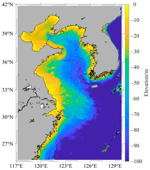
Figure 1.
The elevation of the study area.
2.2. Data
2.2.1. FY-3D Satellite
The FY-3D satellite, designed and launched in 2017 by the China Meteorological Administration (CMA), is a third-generation polar-orbiting meteorological satellite. This study has taken data from the Multi-channel Medium Resolution Spectral Imager-II (MERSI-II) sensor, which captures images of the same target one to two times per day. MERSI-II has 20 spectral bands, including 11 visible and near-infrared bands, and 9 thermal infrared bands, allowing monitoring of complex atmosphere phenomena (e.g., sea fog). This study used the FY-3D MERSI-II Level 1 product with a resolution of 1 km from January 2021 to October 2022. The information of selected channels is shown in Table 1 (http://satellite.nsmc.org.cn/PortalSite/Data/Satellite.aspx, last accessed on: 10 February 2023).

Table 1.
Characteristics of the selected channels of FY-3D MERSI-II used for daytime sea fog detection.
2.2.2. CALIPSO
The CALIPSO (Cloud-Aerosol Lidar and Infrared Pathfinder Satellite Observation) satellite, launched jointly by the National Aeronautics and Space Administration (NASA) and Centre National d’Etudes Spatiales (CNES) in 2006, is equipped with a laser radar instrument called Cloud-Aerosol Lidar with Orthogonal Polarization (CALIOP). This instrument provides backscatter data at 532 nm and 1064 nm, with a horizontal resolution of 1/3 km and a vertical resolution of 30 m below 8.2 km. Backscatter data are processed into a virtual file manager (VFM) product that identifies the horizontal and vertical distribution of clouds and aerosols. The VFM product classifies each layer into eight categories, including invalid, clean atmosphere, cloud, aerosol, stratosphere, surface, subsurface, and no signal. Additional information can be found on the CALIPSO official website (https://www-calipso.larc.nasa.gov/products/, last accessed on: 10 February 2023).
2.3. Methods
2.3.1. Extraction of Sea Fog Labels
CALIPSO backscatter and VFM products are used to identify sea fog events and develop the sea fog detection model. Sea fog labels are extracted through the following approach [13]: First, “cloud” pixels are no more than two pixels away from “surface” pixels in the vertical direction; second, the “surface” and “subsurface” pixels in the VFM data are at least two pixels above the zero-degree elevation of the ocean surface. Sea fog is defined as pixels with a 1064 nm backscatter coefficient greater than 0.025 (km−1·sr−1) and a 532 nm backscatter coefficient greater than 0.03 (km−1·sr−1). In addition, clouds were classified into mid–high-level clouds and low stratus according to their cloud base height. Considering the presence of sub-cloud fog, all target samples were labeled as one of the six categories: clear, sea fog, low stratus, fog below low stratus, mid–high-level clouds, and fog below the mid–high-level clouds. An example of extraction results is shown in Figure 2a.
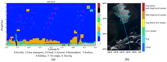
Figure 2.
(a) Sea fog detection results obtained from CALIPSO on 25 March 2021; (b) FY-3D MERSI-II color-composite image with sea fog points extracted by CALIPSO at 05:05 on 25 March 2021, the cyan line represents the extrapolation region of sea fog.
CALIPSO and FY-3D data are matched by a time window of 1 h and a spatial window of 0.02°. Only the closest FY-3D and CALIPSO pair will be retained when there are multiple FY-3D pixels within 0.02° of a CALIPSO pixel. We obtained 1364 observations of sea fog, 3682 observations of low stratus, and 13,696 observations of mid–high-level clouds from January 2021 to October 2022. In comparison with clouds, there was a small amount of sea fog data for classification, which may lead to inaccurate results. This limitation was overcome by visual interpretation of CALIPSO image observations [14]. The pixels we selected were close in location and had similar morphology to those in our sample dataset for detection. An example is Figure 2b, where the cyan line represents the extrapolation region for sea fog. We only extrapolated pixels with obvious features and samples from sea fog and low stratus. We selected 200~300 samples per image to ensure diversity in our sample dataset and prevent an over-reliance on similar samples. Using this method, we were able to obtain 2358 sea fog samples. The number of samples for each type is shown in Table 2.
Table 2.
The number of matching samples between CALIPSO and FY-3D.
2.3.2. Experimental Platform and Supervised Classification Methods
MATLAB is a high-performance numerical computing and visualization software developed by MathWorks that provides various powerful toolboxes (https://www.mathworks.com/products/matlab.html, last accessed on: 22 February 2023). In this study, we used MATLAB R2022a as the experimental platform and employed the Classification Learner App to build and evaluate the performance of daytime sea fog detection model based on four supervised classification algorithms, including Decision Tree (DT), Support Vector Machine (SVM), Nearest Neighbor Classifier, and Neural Network Classifier.
In the Decision Tree (DT) algorithm, data are recursively divided into smaller subsets using the most significant features in the data. In our study, however, the DT algorithm was used to classify clear, sea fog, and cloud pixels. A decision tree was based on the Gini diversity index, which measures the probability of misclassifying a randomly chosen element in each subset.
Support Vector Machine seek to determine which hyperplanes separate the classes in the data most effectively. A key objective of the algorithm is to maximize the margin between the hyperplane and the nearest boundary data points. We used SVM with a Gaussian kernel function in this study, and the data were standardized before model training.
Nearest Neighbor Classifier make predictions based on the class of the closest training data points in the feature space. This used a K-Nearest Neighbor (KNN) model to detect automatic sea fog. The distance weight was configured as an inverse distance. Data standardization was also performed as part of the modeling process.
Neural Network Classifier are a family of models inspired by the human brain structure and functions. For classification, this study trained a fully connected Neural Network. The Neural Network structure has four main components: an input layer, multiple layers of interconnected nodes, the Rectified Linear Unit (ReLU), and an output layer. The algorithm used to train the classifier is backpropagation, which involves propagating the errors from the output layer back through the network to adjust the weights. The weights are adjusted iteratively until the network produces the desired output for a given input. The Neural Network Classifier uses the cross-entropy loss function to measure the difference between the predicted and actual classes, the formula is shown in Equation (1).
where N is the number of samples, is the actual class, and is the predicted class.
In addition to these settings, there are some options called hyperparameters that can significantly affect the supervised classification models. For example, the maximum number of splits in a decision tree. We used hyperparameter optimization within the Classification Learner APP to reduce errors caused by manually selecting hyperparameters. An optimization scheme is used to choose hyperparameter values based on an optimized hyperparameter method that minimizes model classification errors. We used default Bayesian optimization for the optimizer parameters. The automatically optimized hyperparameters are presented in Table 3. More details can be found in the MATLAB help center (https://www.mathworks.com/help/stats/ (accessed on 20 April 2023)).
Table 3.
The automatically optimized hyperparameters in supervised classification.
2.3.3. Evaluation of Model Performance
The performance of each classification algorithm was evaluated using a 10-fold cross-validation strategy [15,16]. The matched CALIPSO sample labels and FY-3D satellite data were divided into 10 groups, where 9 subsets were used for training the model and 1 subset was used for validation. We repeated the process ten times, applying the validation to each subset a single time. As a final step, we average the results of the 10 folds to obtain a validation result for the whole dataset.
Classification models were evaluated by a confusion matrix. In supervised classification, a confusion matrix is used to summarize prediction results by comparing actual and predicted categories of the dataset. Table 4 illustrates the confusion matrix.
Table 4.
Contingency table for fog detection validation.
The probability of detection (POD) and false alarm rate (FAR) were calculated by the confusion matrix to evaluate model performance. Higher POD values indicate that the model is capable of accurately identifying positive cases, and a lower value indicates that positive samples are incorrectly classified as negative. FAR measures the frequency of false positives. A lower value corresponds to a smaller proportion of negative samples that are wrongly classified as positive by the model, indicating a lower false alarms rate [17]. The POD and FAR are calculated by the following two Equations (2) and (3):
3. Analysis of Sea Fog Features Base on FY-3D
3.1. Spectral Characteristics
The spectral average and standard deviation of top-of-atmospheric reflectance and brightness temperature of clear, sea fog, low stratus, fog below low stratus, mid–high-level stratus, and fog below mid–high high-level cloud are displayed in Figure 3. It is noteworthy that a notable difference in the top-of-atmospheric reflectance exists between clear and sea fog/cloud samples. The top-of-atmosphere reflectance of clear samples decreased from 0.47 µm to 1.38 µm, with an average value of less than 0.1 at 0.87 µm. In contrast, sea fog and cloud samples show consistent top-of-atmosphere reflectance results from 0.47 µm to 0.87 µm, with an average value higher than 0.3. Therefore, clear pixels can be identified based on the top-of-atmosphere reflectance at 0.87 µm. Secondly, clouds have a higher top-of-atmosphere reflectance than sea fog and clear samples. However, due to their similar microphysical characteristics, these samples exhibit similar spectral characteristics, which make it difficult to make a direct comparison based on visible reflectance [1]. Notably, the reflectance of sub-cloud fog at the top-of-atmosphere is significantly lower than that of the corresponding cloud. Observations from Himawari-8 have yielded similar results [18].
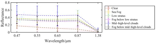
Figure 3.
Top-of-atmosphere reflectance of six target samples (see legend) in the Bohai Sea, Yellow Sea, and East China Sea.
3.2. Brightness Temperature and Brightness Temperature Difference
The distributions of brightness temperature (BT) at 3.80 μm, 7.20 μm, and 10.80 μm are shown in Figure 4. The sea fogs’ brightness temperature (BT3.80: 295.43~317.12 K, with upper quartile-Q3: 310.39 K; lower quartile-Q1: 304.36 K) is higher than the low stratus (287.18~317.59 K, with Q3: 306.40 K; Q1: 298.71 K) and mid–high-level clouds (252.41~321.74 K, with Q3: 304.23 K and Q1: 283.48 K). The observed difference in the brightness temperature between sea fog and clouds may be attributed to the high concentration of water droplets in the sea fog [19]. Lee et al. reported that the shortwave infrared channel (3.9 μm of GOES-8~9) provides a good explanation between liquid clouds (fog/low stratus) and ice clouds (mid–high-level clouds) in satellite images, which supports our findings [20].
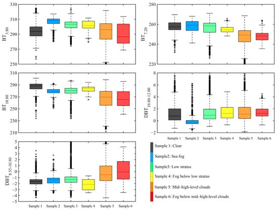
Figure 4.
Boxplots of brightness temperature at 3.80 μm, 7.20 μm, and 10.80 μm; brightness temperature difference between 10.80 μm and 12.00 μm; and brightness temperature difference between 8.55 μm and 10.80 μm of six target samples (see legend), with outliers denoted by “+” symbols.
Sea fog, low stratus, and mid–high-level clouds exhibit a decreasing trend in the BT at 7.20 μm. However, the difference in BT for sea fog (244.24~268.10 K), low stratus (238.32~271.06 K), and clear sky (244.14~269.70 K) samples is small, which makes it difficult to distinguish them directly using a threshold. In contrast, the cloud top height is generally calculated by the BT at 10.80 μm. High BT values indicate clear (cloud-free) areas and relatively low BT values indicate mid–high-level clouds, such as cirrus clouds [21,22]. Figure 4 shows the BT10.80 for mid–high-level clouds ranges from 220.83 K to 298.79 K and 240.85 K to 296.41 K for other cloud types and sea fog. Because of the differences in BT10.80 for clouds, it is possible to distinguish the mid–high-level clouds from other clouds. Sub-cloud fog does not exhibit distinct differences in the brightness temperature. Its values are mostly distributed within the corresponding range of the brightness temperature levels.
Notably, significant differences exist between clear and cloud (including sea fog) samples. Clear samples have lower BT3.80 and BT7.20 than cloud samples, but higher BT10.80 than cloud samples. Therefore, the BT difference between 10.80 μm and 3.80 (or 7.20 μm) for clear samples is higher than for cloud and sea fog samples. The interrelationship between these three channels has been widely used for cloud extraction [23].
However, it is important to note that the clouds and sea fog in the Bohai, Yellow, and East China Sea revealed significant BT differences. A large difference in the brightness temperature (DBT10.80–12.00) is characteristics of cloud samples (−1.84 to 5.08) due to the dissimilar absorption properties of ice crystals in 11.80 μm and 12.00 μm channels [17]. Conversely, most sea fog is composed of water droplets, resulting in a low DBT10.80–12.00 ranging from −1.34 to 0.89 (Figure 4). Moreover, the BT difference between 8.55 μm and 10.80 μm is also related to the cloud phase, with ice clouds and water clouds exhibiting distinct absorption properties between these two channels [24,25]. The DBT8.55–10.80 tends to be a small negative value for sea fog (−3.15~0.14), as depicted in Figure 4. Furthermore, the fog below low stratus shows lower DBT8.55–10.80 values compared to the low stratus and sea fog.
3.3. Texture Features
Sea fog occurs in the Bohai, Yellow, and East China Sea as a result of advection, which is formed by the influx of warm and moist air over a cold sea surface due to upwelling seawater [3]. In contrast to other cloud types, sea fog has a relatively smooth texture in images, which presents a lower brightness temperature variability in the thermal infrared channel. In this study, channel 24 (10.80 μm) is used to evaluate texture smoothness [6]. Figure 5 displays the standard deviation of the brightness temperature (STD BT10.80) within a 5 × 5 moving window for sea fog and cloud regions. The standard deviation of the brightness temperature of sea fog (0.06~0.32) is much lower than that for clouds (0.03~6.21), which provides an effective criterion to distinguish sea fog from other clouds. STD BT10.80 is low below the low stratus (0.04 to 2.29), whereas it is high below the mid–high-level clouds (0.04~5.40).
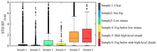
Figure 5.
Boxplots of the standard deviation of brightness temperature at 10.80 μm of six target samples (see legend), with outliers denoted by “+” symbols.
3.4. Auxiliary Parameters
The NDSI measured visible and infrared reflectance to distinguish snow from other land covers [26]. Middle-high clouds, which also contain ice and snow, exhibit similar spectral characteristics to snow [27]. Due to scattering, middle-high clouds have a higher reflectance in the visible wavelength than other cloud types, but a lower reflectance in the shortwave infrared wavelength [5,6], which makes the NDSI of sea fog significantly lower than that of clouds (Figure 6). By using the formula below, the NDSI is calculated from the MERSI-II-based reflectance in channels 1 () and 7 ().
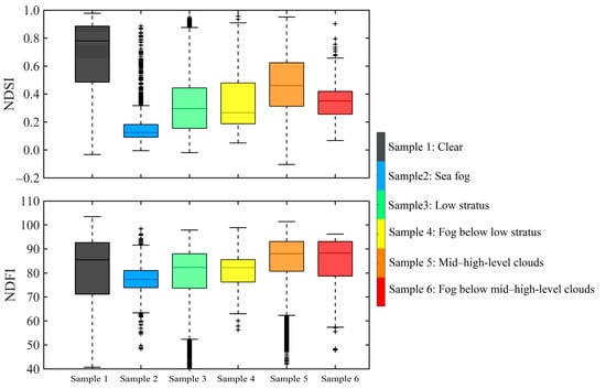
Figure 6.
Boxplots of the normalized difference snow index (NDSI) and normalized difference fog index (NDFI) of six target samples (see legend), with outliers denoted by “+” symbols.
In Figure 6, it can be seen that clear samples have the highest NDSI (−0.03 to 0.98), followed by mid–high-level clouds (−0.10 to 0.95), low stratus (−0.01 to 0.87), sub-cloud fog (0.04 to 0.90), and sea fog (0.00 to 0.32).
The simulation and analysis of sea fog and clouds’ spectral characteristics based on radiative transfer models indicate that sea fog reflectance at 0.65 μm (channel 3) is lower than other cloud types. In contrast, the reflectance at 3.8 μm (channel 20) is higher due to small droplets in fog [7,28]. These findings led Liu et al. (2011) to propose a normalized difference fog index (NDFI) to characterize fog intensity Equation (5):
where and are the albedo and observed radiance of channel 20, respectively. is the Planck function radiance at channel 20, which is calculated using the brightness temperature of channel 24; is the solid angle of the sun to the Earth (6.8 × 10⁻⁵ sr); is the solar zenith angle; and and are the MERSI-II-based reflectance at channels 3 and 20. Clouds and sea fog typically have an NDFI higher than 60, while clear samples have an NDFI between 40.70 and 103.48. MERSI-II monitoring images show low values of NDFI for clear samples due to sun glint. Sea fog’s NDFI varies from 63.41 to 91.59, which is slightly lower than low stratus (52.37~97.87) and mid–high-level clouds (62.34~101.42). This sub-cloud fog has lower NDFI values than cloud samples, which is consistent with sea fog.
4. Automatic Daytime Sea Fog Detection
4.1. Detection Model Construction
FY-3D image features were used as the input to supervised classification models. For each pixel in the image, the corresponding values of the reflectance of the five channels (channel 1~5), brightness temperatures (BT3.8, BT7.20, and BT10.80), brightness temperature difference (DBT10.80–12.00 and DBT8.55–10.80), and the standard deviation of BT10.80, NDSI, and NDFI were extracted. Among these features, the reflectance at 0.87 μm and 1.38 μm, BT3.8, BT7.20, and BT10.80 were used to separate the clear sky from clouds. In contrast, DBT10.80–12.00 and DBT8.55–10.80, and the standard deviation of BT10.80, NDSI, and NDFI were employed to distinguish sea fog from other cloud types. Yet, we were unable to identify any clear feature differences for sub-cloud fog. We used supervised classification to build a daytime sea fog detection model that used a 13-dimensional feature matrix. The model’s output classification results include clear sky, sea fog, low stratus, fog below low stratus, mid–high-level clouds, and fog below mid–high-level clouds. The models are trained for automatic sea fog detection.
The hyperparameter values were automatically selected using the Classification Learner APP to minimize the classification error of the models. We determined the optimal hyperparameters for the DT model at 919 splits and for the SVM model at 95.10 constraint level and 1.40 kernel scale. In the KNN model, the number of neighbors in the KNN model was set to 4. In the Neural Network model, there were three fully connected layers, where approximately 297, 23, and 236 were the sizes of the first, second, and third layers, respectively.
Table 5 shows the results of a 10-fold cross-validation on the four models, based on POD and FAR, to evaluate the effectiveness of the supervised classification methods in detecting sea fog. It was determined that all supervised classification models were capable of extracting clear samples, with a POD of 97.8% estimated by the Neural Network model. However, the FAR was quite high over the six samples, with the average FAR for the clear sample being about 13.9%. For cloud samples, all models exhibited the highest recognition accuracy for mid-to-high clouds, with the SVM achieving the highest POD of 94.7% and DT achieving the lowest POD of 92.8%. The recognition accuracy for low stratus was similar between the SVM, KNN, and Neural Network models, with a POD of 85%~86%. These three models also showed strong sea fog recognition, with POD scores higher than 92.4% and FAR scores lower than 8.7%. Notably, the high precision achieved in the identification of low stratus (POD greater than 85%) and sea fog (POD greater than 92%) demonstrates that supervised classification is effective at distinguishing these phenomena. Even so, when sea fog exists below low clouds, the recognition accuracy of sub-cloud fog is extremely low, with a POD of only 11.6% (KNN). Low stratus has the lowest probability of fog detection, with the highest probability of fog detection of 57.4% (SVM). In light of this, POD and FAR for the supervised classification of clear sky, sea fog, low clouds, and mid–high clouds are relatively high, and the classifications of these four targets are relatively accurate. The challenge is identifying sub-cloud fog, particularly fog below the low stratus.
Table 5.
The probability of detection (POD) and false alarm rate (FAR) for different samples using supervised classification methods.
Among the four supervised classification models, SVM outperforms the other three methods, exhibiting higher PODs and lower FARs. With the exception of clear samples, The Neural Network Classification’s precision is marginally lower than SVMs. The DT model shows the worst performance in identifying different types of targets, especially misjudging low stratus and sub-cloud fog.
4.2. Comparison of Detection Results
The performance of four supervised classification models for sea fog detection in the Yellow Sea was experimentally evaluated from 20–22 May 2022 (Figure 7). Notably, three models (e.g., SVM, KNN, and Neural Network) accurately captured the basic components of the sea fog, and the extracted regions matched the color composite image of the sea fog. The Neural Network Classifier demonstrated better performance at distinguishing cloudy pixels from clear sky pixels, with the lowest misclassification rate. It also detected clouds and sea fog during the sun glint (at 124°E and 32.5°N on 22 May). However, this classifier has limitations for sea fog detection (e.g., misclassification of sea fog); this is especially evident in areas where the sun glint and turbid coastal waters overlap. A misclassification of sea fog may occur because these areas appear like mist in the images and show some similarities in spectral features. The misclassifications could be reduced if these pixels were manually labeled as “clear” pixels in the input samples. Furthermore, sub-cloud fog cannot be detected with any of the four classifiers. There were noticeable clouds within the main part of the sea fog on 20 May, which met the characteristics of fog below mid–high-level clouds. The four models, however, all identify these as mid–high-level clouds. According to the recognition results of the DT model, fog existed below mid–high-level clouds near 124.5°E and 29°N on 22 May; however, this phenomenon is not observed in the color composite image of FY-3D.
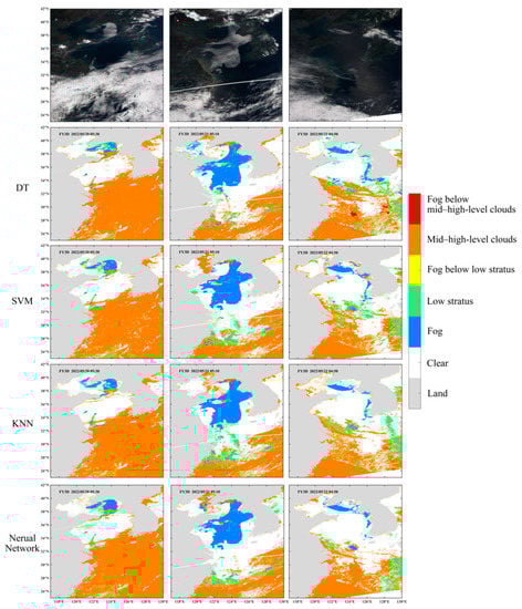
Figure 7.
The color-composite image of FY-3D and sea fog detection results in the Yellow Sea based on Decision Tree (DT), Support Vector Machine (SVM), K-Nearest Neighbor (KNN), and Neural Network Classifier from 20–22 May 2022.
4.3. Analysis of Model Computational Efficiency
The model computational efficiency is a key index to evaluate a model’s performance. According to Table 6, the DT model takes the shortest time to train (i.e., 1.4 min), while the SVM and Neural Network Classifier take the longest time (~697 min). In terms of model application, the SVM model has the longest computation time (i.e., 47.5 min) to classify one scene image, which contradicts the real-time requirements of sea fog detection. In contrast, both DT and NN models take less than one minute. Model accuracy and computational efficiency demonstrate that Neural Network Classifier are superior for detecting sea fog in the daytime.
Table 6.
Time required for model training and application, with application of the model based on FY-3D Imagery from 20–22 May 2022.
5. Discussion
5.1. Feature Selection for Supervised Classification
To detect sea fog, supervised classification methods are commonly employed, where input features are commonly categorized as single- or multi-channel reflectance, and texture features of reflectance. However, some classification methods are driven only by the most accurate single feature for every sub-sample rather than the evaluation measure for the combinatorial feature subset, such as DT, KNN, and SVM [29]. In another way, this means that they do not use the most effective combination of features for classification. Therefore, sea fog and low stratus with similar spectral features may be difficult to distinguish based solely on reflectance, especially when distinguishing sea fog from clouds is the task at hand [1]. On the other hand, texture features can capture local spatial relationship features of an image through measures such as energy, entropy, contrast, etc. Nevertheless, calculating texture features across all channels without selection may not always lead to better classification results if more than 100 dimensions are used as inputs.
To address these issues, we counted the spectral and texture features of sea fog and auxiliary parameters for sea fog detection, which helped to distinguish sea fog from other targets. A 13-dimensional feature matrix was then used to train four sea fog detection classifiers. The 13 dimensions comprise the reflectance of channels 1 to 5, brightness temperature (e.g., BT3.8, BT7.20, and BT10.80), brightness temperature difference (e.g., DBT10.80–12.00 and DBT8.55–10.80), and the standard deviation of BT10.80, NDSI, and NDFI.
Figure 8 presents the rank features for classification obtained through the minimum redundancy maximum relevance (MRMR) algorithm. When the training dataset contains clear samples, the predictor importance scores of BT3.8, BT10.80, and STD BT10.80 are high, while the brightness temperature differences and auxiliary parameters are relatively low. When the task is limited to classifying sea fog from clouds, the predictor importance scores for STD BT10.80, Ref0.55, and DBT8.55–10.80 are high, while the importance rankings of the brightness temperature differences, texture features, and auxiliary parameters have improved, but not for the NDSI. Therefore, we recommend that the brightness temperature differences and auxiliary parameters be incorporated into supervised classification-based sea fog detection to enhance its accuracy.
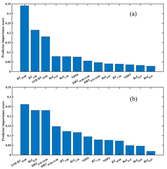
Figure 8.
Rank features for classification using minimum redundancy maximum relevance (MRMR) algorithm. Where (a) is for dataset with clear samples and (b) is for dataset without clear samples.
Retraining the sea fog detection model with different input data was performed with the two most effective classifiers. The classifier settings were the same as in Section 4.1. A significant decrease in detection accuracy was observed for sea fog, low clouds, and sub-cloud fog when only using reflectance values in channels 1–5 (Table 7). As a result, SVM’s POD for sea fog detection decreased from 93.8% to 64.9%, and Neural Network Classifier’s POD decreased from 93.4% to 78.8%. In addition, adding three channels of brightness temperature (BT3.8, BT7.20, and BT10.80) to the input data decreased the sea fog detection accuracy (Table 8). As noted above, the SVM classifier showed a larger decrease than the Neural Network Classifier. These two types of inputs also reduced the classifier’s ability to detect sub-cloud fog, suggesting that the brightness temperature differences and auxiliary parameters may be more important for sub-cloud detection.
Table 7.
The probability of detection (POD) and false alarm rate (FAR) for different samples using supervised classification methods. Here, the input data are reflectance values of channels 1 to 5.
Table 8.
The probability of detection (POD) and false alarm rate (FAR) for different samples using supervised classification methods. Here, the input data are reflectance values of channels 1 to 5 and three channels brightness temperature BT3.8, BT7.20, and BT10.80.
5.2. Misjudgment of Sub-Cloud Fog
CALIPSO identified sub-cloud fog under northwest–southeast-oriented clouds, as shown in Figure 9a. During the daytime, sub-cloud fog possesses characteristics that are intermediate between sea fog and clouds, which might be due to optical sensor limitations. For example, when the cloud layer is relatively thin, the sensor may capture the characteristics of sub-cloud fog. The sensor, however, mostly captures the signals from the highest cloud layer when the cloud layer is thick, making it difficult to distinguish sub-cloud fog characteristics. A supervised classification model performed poorly at identifying the sub-cloud fog due to its inability to distinguish it from other categories. SVM models still misclassify fog below low stratus as low stratus or sea fog, and fog below mid–high-level clouds as mid–high-level clouds, as shown in Table 9. SVM and Neural Network Classifier only identify some segments of sub-cloud fog, predominantly in regions where the cloud is comparatively thin (Figure 9b,c).

Figure 9.
(a) FY-3D MERSI-II color-composite image with labels extracted by CALIPSO, and the detection results based on (b) Support Vector Machine (SVM) and (c) Neural Network Classifier at 05:25 on 16 March 2022.
Table 9.
Contingency table for detection validation of SVM classifiers.
6. Conclusions
This study intends to automatically detect daytime sea fog using four supervised classification techniques (e.g., DT, SVM, KNN, and Neural Network). In this regard, we used FY-3D and CALIPSO images (including clear sky, sea fog, low stratus, fog below low stratus, mid–high-level clouds, and fog below the mid–high-level clouds) from January 2021 to October 2022. The accuracy of the four models was evaluated and compared using a 10-fold cross-validation. The major findings are as follows:
- (1)
- The evaluation results showed that four supervised classification models were capable of identifying the clear sky, with the highest POD (97.8%) reported by the Neural Network model. The SVM, KNN, and Neural Network models showed similar recognition accuracies for low clouds, with PODs of 85%~86%. These three models also accurately distinguished the basic components of sea fog from clouds, with SVM having the highest POD of 93.8%. In this way, our study presents an effective approach to distinguishing sea fog from low stratus.
- (2)
- Moreover, Neural Network Classifier offer the best overall performance for daytime sea fog detection in terms of model accuracy and computational efficiency. However, none of the four classifiers could effectively detect sub-cloud fog. The maximum POD for fog below low stratus was only 11.6% (KNN), and the maximum POD for fog below mid–high-level clouds was only 57.4% (SVM). Moreover, some segments of sub-cloud fog detection are usually only possible when the cloud is quite thin. Therefore, future research should focus on addressing the influence of cloud layers in the vertical direction to improve the accuracy of sub-cloud fog detection.
- (3)
- A study of sea fog features found that there are primarily brightness temperature differences, texture features, and auxiliary parameters that separate sea fog from other cloud types. Furthermore, MRMR shows that adding brightness temperature differences, texture features, and auxiliary parameters can be useful for distinguishing sea fog from clouds. This present study suggests that models should be improved by adding auxiliary parameters to detect sea fog.
Author Contributions
Conceptualization, data curation, methodology, formal analysis, investigation, validation, visualization, writing—original draft, Y.W.; conceptualization, methodology, supervision, investigation, writing—review and editing, Z.Q.; supervision, validation, writing—review and editing, D.Z.; validation, writing—review and editing, M.A.A.; data curation, methodology, investigation, validation, visualization, C.H.; writing—review and editing, Y.Z. and K.L. All authors have read and agreed to the published version of the manuscript.
Funding
This research was funded by the National Natural Science Foundation of China, grant number 41976165, and the pilot program of Fengyun satellite applications (2022), grant number FY-APP-2022.0610.
Data Availability Statement
Data are available on request.
Acknowledgments
The authors are grateful to the National Satellite Meteorological Center and the FENGYUN Satellite Data Center (http://satellite.nsmc.org.cn/PortalSite/Default.aspx (accessed on 20 April 2023)) for providing the FY-3D MERSI II data, and the National Aeronautics and Space Administration (https://ladsweb.modaps.eosdis.nasa.gov/ (accessed on 20 April 2023)) for providing CALIPSO data.
Conflicts of Interest
All the authors declare that there are no personal or financial conflict of interest.
References
- Jeon, J.; Kim, S.; Yang, C. Fundamental Research on Spring Season Daytime Sea Fog Detection Using MODIS in the Yellow Sea. Korean J. Remote Sens. 2016, 32, 339–351. [Google Scholar] [CrossRef]
- Jeon, H.; Kim, S.; Edwin, J.; Yang, C.-S. Sea Fog Identification from GOCI Images Using CNN Transfer Learning Models. Electronics 2020, 9, 311. [Google Scholar] [CrossRef]
- Zhang, S.-P.; Xie, S.-P.; Liu, Q.-Y.; Yang, Y.-Q.; Wang, X.-G.; Ren, Z.-P. Seasonal Variations of Yellow Sea Fog: Observations and Mechanisms. J. Clim. 2009, 22, 6758–6772. [Google Scholar] [CrossRef]
- Bendix, J.; Cermak, J.; Thies, B. New Perspectives in Remote Sensing of Fog and Low Stratus—TERRA/AQUA-MODIS and MSG; Cape Town, South Africa, 2004; p. 5. Available online: https://www.researchgate.net/publication/228860444_New_perspectives_in_remote_sensing_of_fog_and_low_stratus-TERRAAQUA-MODIS_and_MSG (accessed on 20 April 2023).
- Zhang, S.; Yi, L. A Comprehensive Dynamic Threshold Algorithm for Daytime Sea Fog Retrieval over the Chinese Adjacent Seas. Pure Appl. Geophys. 2013, 170, 1931–1944. [Google Scholar] [CrossRef]
- Wu, X.; Li, S. Automatic Sea Fog Detection over Chinese Adjacent Oceans Using Terra/MODIS Data. Int. J. Remote Sens. 2014, 35, 7430–7457. [Google Scholar] [CrossRef]
- Wen, X.; Hu, D.; Dong, X.; Yu, F.; Tan, D.; Li, Z.; Liang, Y.; Xiang, D.; Shen, S.; Hu, C.; et al. An Object-Oriented Daytime Land Fog Detection Approach Based on NDFI and Fractal Dimension Using EOS/MODIS Data. Int. J. Remote Sens. 2014, 35, 4865–4880. [Google Scholar] [CrossRef]
- Ameur, Z.; Ameur, S.; Adane, A.; Sauvageot, H.; Bara, K. Cloud Classification Using the Textural Features of Meteosat Images. Int. J. Remote Sens. 2004, 25, 4491–4503. [Google Scholar] [CrossRef]
- Kim, D.; Park, M.-S.; Park, Y.-J.; Kim, W. Geostationary Ocean Color Imager (GOCI) Marine Fog Detection in Combination with Himawari-8 Based on the Decision Tree. Remote Sens. 2020, 12, 149. [Google Scholar] [CrossRef]
- Tao, L.; Wei, J.; Randi, F.; Gang, L.; Caoqian, Y. Nighttime Sea Fog Recognition Based on Remote Sensing Satellite and Deep Neural Decision Tree. OEE 2022, 49, 220007–220013. [Google Scholar] [CrossRef]
- Jordan, M.I.; Mitchell, T.M. Machine Learning: Trends, Perspectives, and Prospects. Science 2015, 349, 255–260. [Google Scholar] [CrossRef] [PubMed]
- Guyon, I.; Elisseeff, A. An Introduction to Variable and Feature Selection. J. Mach. Learn. Res. 2003, 3, 1157–1182. [Google Scholar]
- Wu, D.; Lu, B.; Zhang, T.; Yan, F. A Method of Detecting Sea Fogs Using CALIOP Data and Its Application to Improve MODIS-Based Sea Fog Detection. J. Quant. Spectrosc. Radiat. Transf. 2015, 153, 88–94. [Google Scholar] [CrossRef]
- Chunyang, Z.; Jianhua, W.; Shanwei, L.; Hui, S.; Xiao, Y. Sea Fog Detection Using U-Net Deep Learning Model Based on Modis Data. In Proceedings of the 2019 10th Workshop on Hyperspectral Imaging and Signal Processing: Evolution in Remote Sensing (WHISPERS), Amsterdam, The Netherlands, 24–26 September 2019; pp. 1–5. [Google Scholar]
- Kang, Y.; Kim, M.; Kang, E.; Cho, D.; Im, J. Improved Retrievals of Aerosol Optical Depth and Fine Mode Fraction from GOCI Geostationary Satellite Data Using Machine Learning over East Asia. ISPRS J. Photogramm. Remote Sens. 2022, 183, 253–268. [Google Scholar] [CrossRef]
- Hastie, T.; Tibshirani, R.; Friedman, J.H.; Friedman, J.H. The Elements of Statistical Learning: Data Mining, Inference, and Prediction; Springer: Berlin/Heidelberg, Germany, 2009; Volume 2. [Google Scholar]
- Han, J.H.; Suh, M.S.; Yu, H.Y.; Roh, N.Y. Development of Fog Detection Algorithm Using GK2A/AMI and Ground Data. Remote Sens. 2020, 12, 3181. [Google Scholar] [CrossRef]
- Hu, C.; Qiu, Z.; Liao, K.; Zhao, D.; Wu, D. CALIOP Remote Sensing Monitoring of Fujian Sea Fog and Spectral Characteristics Analysis of Subcloud Fog Based on Himawari-8. J. Trop. Oceanogr. 2022. [Google Scholar] [CrossRef]
- Allen, R.C.; Durkee, P.A.; Wash, C.H. Snow/Cloud Discrimination with Multispectral Satellite Measurements. J. Appl. Meteor. 1990, 29, 994–1004. [Google Scholar] [CrossRef]
- Lee, T.F.; Turk, F.J.; Richardson, K. Stratus and Fog Products Using GOES-8–9 3.9-Μm Data. Weather Forecast. 1997, 12, 664–677. [Google Scholar] [CrossRef]
- Inoue, T. On the Temperature and Effective Emissivity Determination of Semi-Transparent Cirrus Clouds by Bi-Spectral Measurements in the 10μm Window Region. J. Meteorol. Soc. Jpn. 1985, 63, 88–99. [Google Scholar] [CrossRef]
- Giannakos, A.; Feidas, H. Classification of Convective and Stratiform Rain Based on the Spectral and Textural Features of Meteosat Second Generation Infrared Data. Theor. Appl. Climatol. 2013, 113, 495–510. [Google Scholar] [CrossRef]
- Ackerman, S.A.; Holz, R.E.; Frey, R.; Eloranta, E.W.; Maddux, B.C.; McGill, M. Cloud Detection with MODIS. Part II: Validation. J. Atmos. Ocean. Technol. 2008, 25, 1073–1086. [Google Scholar] [CrossRef]
- Qu, J.J.; Gao, W.; Kafatos, M.; Murphy, R.E.; Salomonson, V.V. (Eds.) Earth Science Satellite Remote Sensing; Springer: Berlin/Heidelberg, Germany; Tsinghua University Press: Beijing, China, 2006; ISBN 978-3-540-35837-4. [Google Scholar]
- Thies, B.; Nauß, T.; Bendix, J. Precipitation Process and Rainfall Intensity Differentiation Using Meteosat Second Generation Spinning Enhanced Visible and Infrared Imager Data. J. Geophys. Res. Atmos. 2008, 113. [Google Scholar] [CrossRef]
- Dozier, J.; Painter, T.H. Multispectral and Hyperspectral Remote Sensing of Alpine Snow Properties. Annu. Rev. Earth Planet. Sci. 2004, 32, 465–494. [Google Scholar] [CrossRef]
- Wielicki, B.A.; Barkstrom, B.R.; Harrison, E.F. Clouds and the Earth’s Radiant Energy System (CERES): An Earth Observing System Experiment. Bull. Am. Meteorol. Soc. 1996, 77, 853–868. [Google Scholar] [CrossRef]
- Liu, L.; Wen, X.; Gonzalez, A.; Tan, D.; Du, J.; Liang, Y.; Li, W.; Fan, D.; Sun, K.; Dong, P.; et al. An Object-Oriented Daytime Land-Fog-Detection Approach Based on the Mean-Shift and Full Lambda-Schedule Algorithms Using EOS/MODIS Data. Int. J. Remote Sens. 2011, 32, 4769–4785. [Google Scholar] [CrossRef]
- Wang, Y.Y.; Li, J. Feature-selection Ability of the Decision-tree Algorithm and the Impact of Feature-selection/Extraction on Decision-tree Results Based on Hyperspectral Data. Int. J. Remote Sens. 2008, 29, 2993–3010. [Google Scholar] [CrossRef]


Disclaimer/Publisher’s Note: The statements, opinions and data contained in all publications are solely those of the individual author(s) and contributor(s) and not of MDPI and/or the editor(s). MDPI and/or the editor(s) disclaim responsibility for any injury to people or property resulting from any ideas, methods, instructions or products referred to in the content. |
© 2023 by the authors. Licensee MDPI, Basel, Switzerland. This article is an open access article distributed under the terms and conditions of the Creative Commons Attribution (CC BY) license (https://creativecommons.org/licenses/by/4.0/).