Assessing the Accuracy and Consistency of Six Fine-Resolution Global Land Cover Products Using a Novel Stratified Random Sampling Validation Dataset

Abstract

Over the past decades, benefiting from the development of computing capacity and the free access to Landsat and Sentinel imagery, several fine-resolution global land cover (GLC) products (with a resolution of 10 m or 30 m) have been developed (GlobeLand30, FROM-GLC30, GLC_FCS30, FROM-GLC10, European Space Agency (ESA) WorldCover and ESRI Land Cover). However, there is still a lack of consistency analysis or comprehensive accuracy assessment using a common validation dataset for these GLC products. In this study, a novel stratified random sampling GLC validation dataset (SRS_Val) containing 79,112 validation samples was developed using a visual interpretation method, significantly increasing the number of samples of heterogeneous regions and rare land-cover types. Then, we quantitatively assessed the accuracy of these six GLC products using the developed SRS_Val dataset at global and regional scales. The results reveal that ESA WorldCover achieved the highest overall accuracy (of 70.54% ± 9%) among the global 10 m land cover products, followed by FROM-GLC10 (68.95% ± 8%) and ESRI Land Cover (58.90% ± 7%) and that GLC_FCS30 had the best overall accuracy (of 72.55% ± 9%) among the global 30 m land cover datasets, followed by GlobeLand30 (69.96% ± 9%) and FROM-GLC30 (66.30% ± 8%). The mapping accuracy of the GLC products decreased significantly with the increased heterogeneity of landscapes, and all GLC products had poor mapping accuracies in countries with heterogeneous landscapes, such as some countries in Central and Southern Africa. Finally, we investigated the consistency of six GLC products from the perspective of area distributions and spatial patterns. It was found that the area consistencies between the five GLC products (except ESRI Land Cover) were greater than 85% and that the six GLC products showed large discrepancies in area consistency for grassland, shrubland, wetlands and bare land. In terms of spatial patterns, the totally inconsistent pixel proportions of the 10 m and 30 m GLC products were 23.58% and 14.12%, respectively, and these inconsistent pixels were mainly distributed in transition zones, complex terrains regions, heterogeneous landscapes, or mixed land-cover types. Therefore, the SRS_Val dataset well supports the quantitative evaluation of fine-resolution GLC products, and the assessment results provide users with quantitative metrics to select GLC products suitable for their needs.

1. Introduction

Land cover, as a key biophysical driver for earth system models, is essential for hydrological modeling [1,2], climate modeling [3,4], and earth system modeling [5,6], and also plays an important role in biodiversity conservation [7,8] and carbon cycles [9,10,11].

Recently, with the free access to open satellite archives and the advent of low-cost cloud computing capabilities, great progress has been made in global land cover (GLC) mapping at fine spatial resolutions (10 m or 30 m) over the past few years [12,13,14]. At present, seven global 10 m or 30 m land cover mapping products have been released, including three 30 m GLC products (GlobeLand30 [15], FROM-GLC30 [16], GLC_FCS30 [17]) and four 10 m GLC products (FROM-GLC10 [18], European Space Agency (ESA) WorldCover [19], ESRI Land Cover [12] and Dynamic World [13]). Among them, Dynamic World is a near-real-time dataset paralleled with Sentinel-2 acquisitions. The 2020 Dynamic World GLC map needs to be aggregated using some compositing methods, such as mean, median, and mode [20]. This leads to the accuracy of the results being constrained by classification performance and compositing methods for Dynamic World products. Therefore, Dynamic World was excluded from the GLC products assessed.

Table 1. Summary of the six fine-resolution global land cover datasets to be assessed in this study.

	European Space Agency (ESA) WorldCover	ESRI Land Cover	FROM-GLC10	GlobeLand30	FROM-GLC30	GLC_FCS30
Simplification	ESA_WC	ESRI_LC	FROM-GLC10	GlobeLand30	FROM-GLC30	GLC_FCS30
Organization	European Space Agency	Environmental Systems Research Institute	Tsinghua University	National Geomatics Center of China	Tsinghua University	Chinese Academy of Sciences
Sensor/Data Source	Sentinel-1/Sentinel-2	Sentinel-2	Sentinel-2	Landsat TM/ETM+, HJ-1 A/B	Landsat TM/ETM+/OLI	Landsat TM/ETM+/OLI
Spatial Resolution	10	10	10	30	30	30
Time range	2020	2017–2021	2017	2000, 2010, 2020	2015	1985–2020
Method	Random forest	Deep learning segmentation model	Random forest	POK (pixel-object-knowledge-based strategy)	Random forest	Local random forest
Classification System	11 classes	10 classes	10 classes	10 classes	26 classes	29 classes
Overall Accuracy	0.744	0.850	0.728	0.803	0.773	0.825
Access	https://zenodo.org/record/5571936, accessed on 25 January 2023	https://www.arcgis.com/apps/instant/media/index.html?appid=fc92d38533d440078f17678ebc20e8e2, accessed on 25 January 2023	http://data.ess.tsinghua.edu.cn/fromglc10_2017v01.html, accessed on 25 January 2023	http://www.globallandcover.com/, accessed on 25 January 2023	http://data.ess.tsinghua.edu.cn/fromglc2015_v1.html, accessed on 25 January 2023	https://doi.org/10.5281/zenodo.3986872, accessed on 25 January 2023
Reference	Zanaga, et al. [19]	Karra, et al. [12]	Gong, et al. [18]	Chen, et al. [15]	Gong, et al. [16]	Zhang, et al. [17]

gives details of the six available fine-resolution GLC products, including the data source used, classification system, classification method, and reported accuracy. It has been found, using different classification systems, that these GLC products have an overall accuracy ranging from 0.728 to 0.85. However, it should be emphasized that they were independently validated against different validation datasets, that is, and these reported accuracies are incomparable. Consequently, a quantitative assessment of the accuracy and consistency of these GLC products under a common standard is vital for users, in enabling them to select the GLC products that best fit their applications.

The greatest difficulty in comprehensively assessing different GLC products using a common standard is the lack of a free-access and high-quality global validation dataset [21]. The collection of GLC validation datasets is usually expensive, labor-intensive, and time-consuming. Over the past years, several scientists have contributed a great deal of effort to build common validation datasets at regional and global scales [21,22,23,24,25]. For example, more than 250,000 samples in the Land Use/Cover Area Frame Survey were collected throughout the European Union using a two-phase sampling method and photointerpretation (aerial or satellite) [22]. The US Geological Survey Land Change Monitoring, Assessment, and Projection project team developed a TimeSync tool to interpret annual Landsat imageries, and collected 24,971 random samples [23]. These two regional validation datasets, derived from two official institutions, give high confidence when validating various land cover products. However, they are still not suitable for assessing the accuracy of GLC products at a global scale. Some GLC validation datasets have been developed by crowdsourcing data collection or visual interpretation [25,26,27]. For example, Geo-Wiki, collected by crowdsourced interpretation of volunteered geographic information, has the potential to build an up-to-date validation dataset [24]. However, the quality of Geo-Wiki cannot be guaranteed and the data processing is cumbersome because many of the volunteers who contribute to Geo-Wiki lack professional knowledge [28]. A global validation dataset containing 38,664 samples was established in 2014 by combining Landsat images, MODIS Enhanced Vegetation Index time series data and high-resolution images from Google Earth using the visual interpretation method [25]. However, this validation dataset was not subsequently updated in time to evaluate the latest GLC products. Therefore, there are still not enough global validation datasets to assess the accuracy of various GLC products.

The accuracy assessment of different GLC products places rigorous requirements on the generation of validation datasets [29]. It was proposed that the sample allocation process should be independent [27]; that is, this process must be independent of land-cover types in GLC products, and that there should be a flexible classification system and an adjustable sampling scheme. It was also emphasized that the sample allocation should be focused on heterogeneous landscapes with poor mapping accuracy of GLC products [21]. As required to validate different GLC products, sample collection should be a transparent, quality-assured, and reproducible process [29]. However, these rigorous requirements have not been fully considered in the creation of existing validation datasets.

Several studies have couducted accuracy assessment and consistency analysis on various GLC products [20,30,31,32,33,34,35,36]. Liu, et al. [36] have reviewed the accuracy metrics of GlobeLand30, FROM-GLC30 and GLC_FCS30 in different regions and further analyzed their consistency from area and spatial perspectives. Jun, et al. [34] and Kang, et al. [35] analyzed the discrepancies in accuracy and spatial distribution of three 10 m GLC products (FROM-GLC10, ESA_WC and ESRI_LC) in Southwest China and Northwestern China, respectively. Unfortunately, current accuracy assessments and consistency analyses of different GLC products are only available at a regional scale. To date, little effort has been put forward by scientists to evaluate the performance of six available 10 m or 30 m GLC products, especially at a global scale. Therefore, it is critical to conduct comprehensive accuracy assessments and consistency analysis of the available 10 m or 30 m GLC products.

Currently, there is a lack of common validation datasets for the accuracy assessment and consistency analysis of fine-resolution GLC products. In this study, we developed a novel stratified random sampling GLC validation dataset (SRS_Val) using a visual interpretation method and evaluated the land cover interpretation uncertainty of the samples in the SRS_Val dataset. Then, we comprehensively assessed the accuracy of six GLC products (GlobeLand30, FROM-GLC30, GLC_FCS30, FROM-GLC10, ESA_WC and ESRI_LC) using the SRS_Val dataset at global, national, and continental scales, respectively. Lastly, we analyzed the consistencies of six GLC products from area-based and spatial-based perspectives. The assessment of accuracy and consistency of the six GLC products is extremely important for users, to enable them to select the optimal land cover products for their applications.

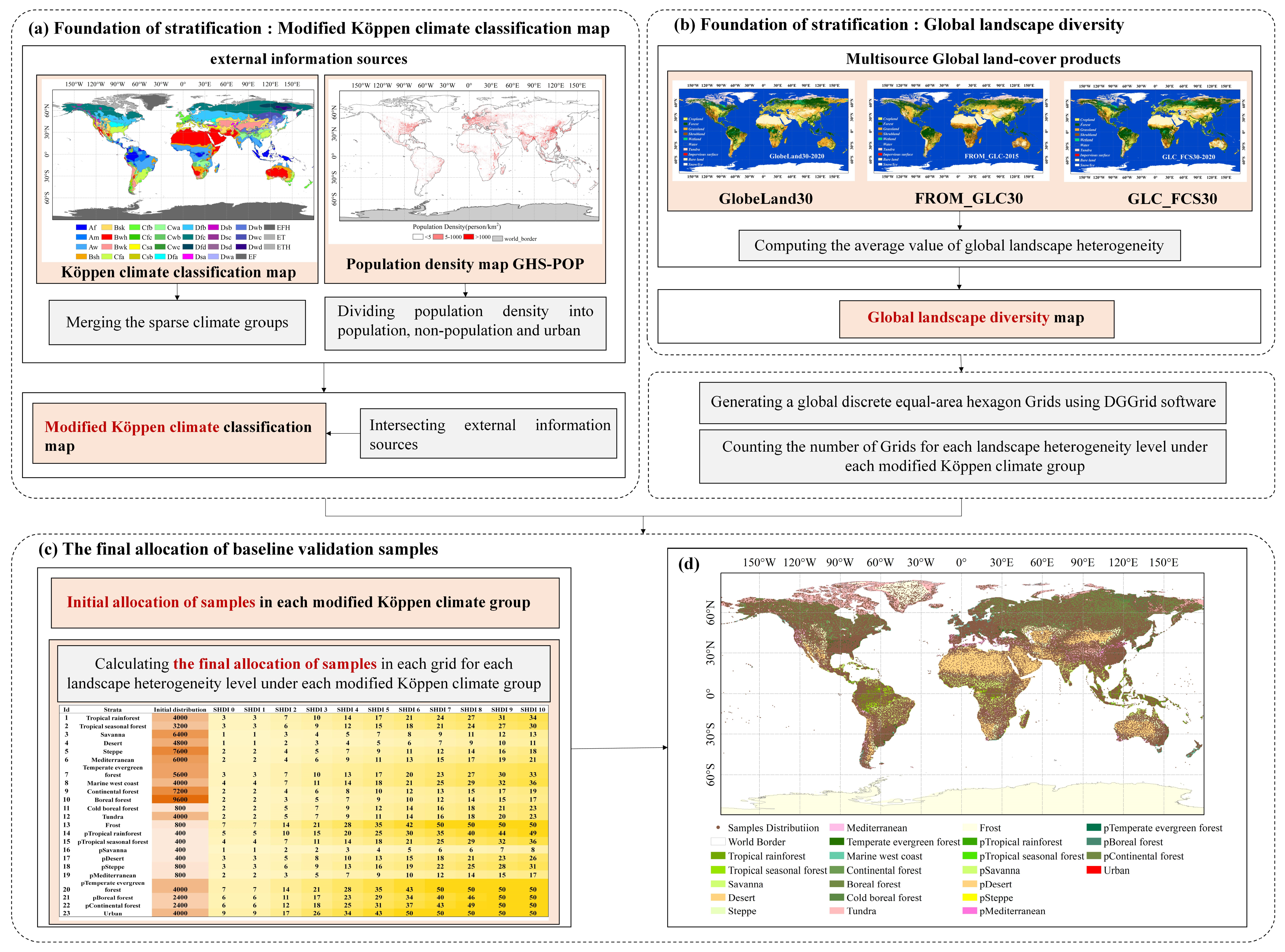
2. The Stratified Random Sampling GLC Validation Dataset (SRS_Val)

A stratified random sampling GLC validation dataset (SRS_Val) was developed to validate six available 10 m or 30 m GLC products. Specifically, we firstly defined a standardized classification system for the SRS_Val dataset (Section 2.1), inherited from the UN Land Cover Classification System (UN-LCCS), which comprised 16 land-cover types. Then, we combined a stratified equal-area sampling design and multisource datasets to allocate the validation samples (Section 2.2). Lastly, we independently visually labeled the SRS_Val dataset using the dedicated interpretation tool and auxiliray imagery, and quality-controlled it based on duplicate interpretations (Section 2.3).

2.1. Land Cover Standardized Classification System for SRS_Val Dataset

In this study, the SRS_Val dataset employed a standardized classification system, derived from the UN-LCCS, which is an international common land cover classification system and is flexible for legend translation [37]. The standardized classification system overcomes limitations of compatibility and comparability between the SRS_Val dataset and the six GLC products; this is crucial for the subsequent harmonization of independent classification systems of six GLC products. The standardized classification system, originally designed to contain 22 LCCS land-cover types (Table S4), was eventually simplified to give the 16 LCCS land-cover types listed in

Table 2. The description of standardized land cover classification system in the SRS_Val dataset.

Label	Description	Label	Description
10	Rain-fed cropland	130	Grassland
20	Irrigated cropland	140	Lichens and mosses
50	Evergreen broadleaved forest	150	Sparse vegetation (fc < 0.15)
60	Deciduous broadleaved forest	180	Wetlands
70	Evergreen needleaved forest	190	Impervious surfaces
80	Deciduous needleaved forest	200	Bare areas
90	Mixed forest	210	Water body
120	Shrubland	220	Permanent snow/ice

by removing some mosaic land-cover types (including mosaic natural vegetation and cropland and mosaic forest and grass or shrubland) and merging some ambiguous land-cover types (including tree–shrub–herbaceous cover, flooded, and fresh/saline or brackish water). These mosaic land-cover types were removed because they could be clearly identified on 10 m or 30 m remote sensing imagery and high-resolution images of Google Earth Pro. The ambiguous land-cover types further merged wetlands land-cover type, as finer classification of wetlands with high spatial and spectral heterogeneity can bring subjective errors in visual interpretation.

2.2. Allocating Validation Samples Using Stratified Equal-Area Sampling Method

An accurate and representative GLC validation dataset collected for the year 2020 (taking into consideration the timeliness of GLC products) was used as a basis for evaluating the performance of the six GLC products. The stratified sampling method has been demonstrated as having a good ability to enhance the sample size of targeted land-cover types by creating unequal inclusion probabilities [38]. Thus, we adopted the stratified equal-area sampling method to increase the validation sample size for some rare land-cover types (such as wetland and impervious surfaces), and simultaneously increase the sample density in heterogeneous landscapes. Furthermore, we applied a global gridding method to estimate the approximate area of various land-cover types. Figure 1 illustrates the detailed workflow for allocating SRS_Val samples using the stratified equal-area random sampling strategy. There were three main steps: application of stratification, design of sampling grids, and allocation of validation samples.

Firstly, the sample allocation process is expected to focus on strata in which some land-cover types that are more likely to be misclassified [27]. Therefore, we adopted three external sources of information, including the Köppen climate groups, population density and landscape heterogeneity patterns, to increase the validation sample size in some rare land-cover types and heterogeneous landscapes. Specifically, the Köppen climate groups (natural drivers of climate) led to a distribution of natural land covers, and the population density (an anthropogenic driver of human disturbance) created complex human-shaped landscapes with a mix of different land covers. Therefore, the modified Köppen climate groups were obtained by the intersection of Köppen climatic groups and population density to enhance the possibility of samples being allocated to regions with high human activity. Given that the modified Köppen climate groups cannot achieve the purpose of expanding the sample density in the heterogeneous landscapes, the Shannon heterogeneity index (SHDI) [39] was introduced into the stratification to reflect the uneven distribution of land-cover types, and its formula was shown in Equation (1). The purpose of stratification is to create the option to allocate the sample size to strata. The targeted land-cover types were generally associated with one or more strata. Therefore, we assigned larger weights to the associated strata to achieve the goal of increasing the sample size of rare land-cover types and heterogeneous landscapes.

$$\mathrm{S}\mathrm{H}\mathrm{D}\mathrm{I}=-{\sum }_{i=1}^m\left(p_i\mathrm{l}\mathrm{n}{p}_i\right)$$

(1)

where m is the number of land-cover types in the window and $p_i$ is the proportion of land-cover type i in the window. We calculated SHDI of the three 30 m GLC products taking 200 km as the window size. Because the 30 m GLC products had goods representations of landscape heterogeneity on the earth’s land surface, the average SHDI value obtained was divided into 11 levels according to quantiles as the stratification basis.

Next, to achieve the goal of estimating the approximate actual area of various land-cover types, we needed to sample the entire land systematically. We applied a global gridding method where the grid unit was an equal-area hexagon, to divide the global land area, which was adopted and recommended by Gong, et al. [16]. Therefore, the global land area (except Antarctica) was divided into 6550 equal-area hexagons. Such a global gridding method can satisfy the randomness of the global spatial distribution and avoid the potential bias of duplication of land cover distributions. Simultaneously, the land area represented by each sample can also be determined.

Finally, the reasonable allocation of validation samples in each hexagon and the realization of a good global distribution of samples are vital, given the multisource stratification method used in the first step. The initial sample size of 80,000 samples was firstly determined according to the following Equation (2) provided by Pontus Olofsson [38] and the different weights of modified Köppen climate groups involved in Olofsson, et al. [27]. Additionally, the sample size in each modified Köppen climate group was calculated using Equation (3).

$$n=\frac{{\left(\sum W_h\sqrt{p_h(1-p_h)}\right)}^2}{V+\sum W_h{P}_h(1-P_h)/N}$$

(2)

$$n_h=n{W}_h$$

(3)

where $N$ is the global size; $W_h$ is the weight on stratum $h$; $p_h$ is the estimated accuracy on stratum $h$; $V={\left(d/t\right)}^2$; d is the absolute error limit of 0.1, and t is the critical value of the standard normal distribution when the confidence level is $1-\mathsf{\alpha }/2$, which is 2.33 when $\alpha$ is 0.025. Then, the number of grids for each landscape heterogeneity level under each modified Köppen climate group was counted, and their weighted proportions were used to determine the weights when we allocated the samples. Finally, after considering the affordable workloads, the collection of 2–50 samples in each hexagon was recommended over the whole globe. The details of sample size determination in each hexagon are given in Supplementary A. The final validation dataset contains 79,112 baseline samples allocated around the globe in Figure 1d.

2.3. Labeling and Quality-Controlling SRS_Val Dataset Using Visual Interpretation Method

To facilitate the collection of validation samples, we developed a dedicated interpretation tool based on the Google Earth Engine platform. This tool provides access to multisource remote sensing satellite data and helps label land-cover types (Figure 2). The data sources used for interpretation include high-resolution Google Maps and Sentinel-2 and Landsat imageries. Simultaneously, the interpretation tool is supplemented with multisource remote sensing auxiliary data (phenological curves, tree height, vegetation coverage, and terrain characteristics) to increase the reliability of the interpretation process. Specifically, these auxiliary data had their specific functions: (1) phenological information was added to complement the fragile visual interpretation of single-date imagery, such as the normalized difference vegetation index time series (used to distinguish vegetation types) and the normalized difference snow index time series (used to define and distinguish snow or ice); (2) the global tree height data [40] was collected to help distinguish shrubland and forest; (3) the vegetation coverage also played an important role in the discrimination between sparse vegetation (which is defined as vegetation with less than 15% vegetation coverage) and grassland; (4) the terrain characteristics (such as elevation and slope) were also critical to revealing the vertical zonality of the vegetation distribution.

The land-cover type of each validation sample was determined based on the independent judgment of each interpreter. In total, 30 junior interpreters and 5 senior experts (with experience in satellite-based land cover analysis and image interpretation) were involved in the interpretation process. Remote training tutorials were first conducted to train the junior interpreters in using the interpretation tools and understanding land-cover type definitions. These interpreters were requested to independently interpret the same set of samples with typical land-cover types, and then experts gave feedback on their interpretations. The aim was to reduce interpretation discrepancies between the interpreters. Figure 3 displays the main processes involved in the quality control of the SRS_Val dataset. Specifically, after interpreters were trained in-depth, the validation samples were divided into about 400 groups, with 200 samples in each group. Each group of samples was independently labeled by three junior interpreters using the dedicated interpretation tool in the first round. Simultaneously, the interpretation confidence levels were also recorded (i.e., unsure, bit sure, sure, quite sure). Next, the interpreted samples were double-checked by five senior experts. Finally, the most experienced experts conducted the final quality control, that is, to review all samples to ensure that they could be interpreted under a common standard.

3. Assessing Accuracy and Consistency of six GLC Products

3.1. Harmonization of Classification Systems for Six GLC Products

As the land cover classification systems of the six GLC products are inconsistent, directly adopting mutual attribution methods without using a common land cover language and a strict set of specific classifiers can lead to potential problems. How to harmonize the difference in the classification system between the SRS_Val dataset and the six GLC products is a crucial precondition for facilitating comprehensive accuracy assessment. The generalized global land cover classification system with 10 basic land-cover types defined by the LCCS classification scheme was used as an ontology. We transformed the classificaton systems of the six GLC products and the SRS_Val dataset to the generalized classification system based on a set of common classifiers (

Table 3. Generalized classification system inherited from LCCS classification scheme and corresponding land-cover types from the six GLC products.

Generalized Land-Cover Type	Simplified Label	LCCS-Code	Validation Dataset	GlobeLand30	FROM-GLC30	GLC_FCS30	FROM-GLC10	ESA _WC	ESRI_LC
Cropland	CRP	A11-A3/A23-A1	10, 20	10	11, 12, 14, 15	10, 11, 12, 20	10	40	5
Forest	FST	A12-A3//A11-A1//A24-A3C1(C2) R1(R2)	50, 60, 70, 80, 90	20	21, 22, 23, 24, 25, 26	50, 60, 61, 62, 70, 71, 72, 80, 81, 82, 90	20	10	2
Grassland	GRS	A12-A2	130	30	31, 32, 33	130	30	30	3
Shrubland	SHR	A12-A4//A11-A2	120	40	41, 42	120, 121, 122	40	20	6
Wetlands	WET	A24-A1(A2/A4/A6)	180	50	51, 52, 53	180	50	90, 95	4
Water body	WAT	B27-A1//B28-A1	210	60	60	210	60	80	1
Tundra	TUN	A12-A7	140	70	70	140	70	100
Impervious surface	IMP	B15	190	80	80	190	80	50	7
Bare land	BAL	B16-A1(A2)//B15-A2	150, 200, 201, 202	90	90	150, 152, 153, 200, 201, 202	90	60	8
Snow/Ice	SNI	B27-A2(A3)//B28-A2(A3)	220	100	101, 102	220	100	70	9

Note: For the names of land-cover type labels of each GLC product, please refer to Tables S5–S10 in Supplementary B. The LCCS-Code, which definition follows the LCCS hierarchy, contains the dichotomous label first and the modular hierarchical second (e.g., B27-A1). The dichotomous label contains three identifiers: the differentiation between vegetated/non-vegetated (A or B), terrestrial or aquatic/regularly flooded (1 or 2), and the differentiation of cultivation/artificial or natural/semi-natural (1–8).

).

Figure 4 shows the spatial distributions of the six GLC products after harmonizing to the generalized classification system. Overall, there was significant consistency among these six GLC products because they basically reflected the spatial pattern of global land cover. Specifically, the forest was mainly concentrated on the tropics and the northern part of the northern hemisphere, and the cropland was mainly distributed on the plains with plenty of rain. However, the discrepancies of the six GLC products were also evident, especially for the ESRI_LC. It can be seen that the ESRI_LC had the largest shrubland areas than other products especially in Australia, Africa and the Middle East, which meant the ESRI_LC misclassified some grassland and bare land regions as shrubland.

3.2. Accuracy Assessment Metrics

The independence of the global validation dataset brought an obsession of mismatch between map land-cover types and sampling strata. Therefore, unequal inclusion probabilities from the stratified random design were incorporated in the sample-based estimates using the indicator variable formulation of the estimators [41]. The overall accuracy (O.A.) was defined as:

$$O.A.={\sum }_{h=1}^H{N}_h{\stackrel{-}{y}}_h/N$$

(4)

where H is the number of strata (H = 253), $N_h$ is the population size of stratum h, N is the total number of sample pixels, and ${\stackrel{-}{y}}_h=\sum _{u\in h}{y}_u/n_h$ is the sample proportion of correctly classified pixels in stratum h. The user’s accuracy (U.A.) and producer’s accuracy (P.A.) were estimated using the ratio estimator $\widehat{R}$.

$$\widehat{R}=\frac{\widehat{Y}}{\widehat{X}}=\frac{{\sum }_{h=1}^H{N}_h{\stackrel{-}{y}}_h}{{\sum }_{h=1}^H{N_h\stackrel{-}{x}}_h}$$

(5)

where $\widehat{R}$ is the proportion of the total number of pixels that are correctly classified as class k (map or reference) and the total number of pixels in class k.

The estimators of the variance of O.A. and $\widehat{R}$ (which was used to calculate the variance estimation of P.A. and U.A.) are:

$$\widehat{V}\left(\widehat{\stackrel{-}{Y}}\right)=\left(\frac{1}{N^2}\right)\left[{\sum }_{h=1}^H{N}_h^2\left(1-\frac{n_h}{N_h}\right)s_{yh}^2/n_h\right]$$

(6)

$$\widehat{V}\left(\widehat{R}\right)=\left(\frac{1}{{\widehat{X}}^2}\right)\left[{\sum }_{h=1}^H{N}_h^2\left(1-\frac{n_h}{N_h}\right)\left(s_{yh}^2+{\widehat{R}}^2{s}_{xh}^2-2\widehat{R}{s}_{xyh}\right)/n_h\right]$$

(7)

where $n_h$ is the sample size in stratum h, $s_{yh}^2$ and $s_{xh}^2$ are the sample variances for yu and xu for stratum h and $s_{xyh}$ is the sample covariance for yu and xu for stratum h.

3.3. Consistency Assessment Metrics

To comprehensively understand the performance of the six GLC products, two aspects need to be addressed: area-based and spatial-based consistency analyses. The area-based consistency analysis was primarily concerned with the area proportion of all land-cover types and the similarities of the same land-cover type between different GLC products. The spatial-based analysis illustrated the spatial consistency of all GLC products at the same location.

3.3.1. Calculating Area-Based Consistency Coefficient

The area-based analysis focused on correlation of the area proportions of each land-cover type between the six GLC products [30,42]. We summarized the area of each land-cover type in each GLC product and then calculated the correlation coefficient of the same land-cover type in different products. The area correlation coefficient is defined as

$$R_{XY}=\frac{\sum _{i=1}^n\left(X_i-\stackrel{-}{X}\right)\left(Y_i-\stackrel{-}{Y}\right)}{\sqrt{\sum _{i=1}^n{\left(X_i-\stackrel{-}{X}\right)}^2\sum _{i=1}^n{\left(Y_i-\stackrel{-}{Y}\right)}^2}}$$

(8)

where R_XY is the area correlation coefficient between GLC products X and Y; i is the land-cover type; X_i and Y_i are the total areas of land-cover type i in land cover products X and Y, respectively; $\stackrel{-}{X}$ and $\stackrel{-}{Y}$ are the averages of the total area of all land-cover types in land cover products X and Y, respectively; and n is the total number of land-cover types.

3.3.2. Applying Spatial-Based Consistency Methods

In terms of spatial consistency, two qualitative methods were applied: the spatial superposition method and the information entropy method. Specifically, the spatial superposition method can obtain the pixel-by-pixel spatial correspondence for different products. Thus, it was commonly employed to acquire the spatial agreement when using a small number of land-cover products [30,43,44]. We applied the method to obtain the spatial consistency between three 10 m GLC products and between three 30 m GLC products, respectively. The degree of spatial consistency between three GLC products was classified as high consistency (i.e., three GLC products shared same labels), moderate consistency (i.e., only two GLC products owned same labels), or low consistency (i.e., three GLC products had different labels).

However, the discrete measure obtained by applying the spatial superposition method will be too complicated when we want to comprehensively analyze the spatial consistency of the six GLC products. To better quantify the degree of complex spatial consistency among the six GLC products, the information entropy method was employed, which was commonly used to obtain spatial correspondence map between multiple GLC maps in some studies [45,46]. We counted the number of consistent groups between GLC products pixel by pixel, and then calculated the normalized information entropy (Equation (9)). If among the six GLC products, three products agree between themselves, two products agree with each other, and one product does not agree with any other product, then m = 3, p₁ = $3/6$, p₂ = $2/6$, p₃ = $1/6$.

$$\mathrm{E}\mathrm{n}\mathrm{t}\mathrm{r}\mathrm{o}\mathrm{p}\mathrm{y}=-{\sum }_{i=1}^m\left(p_i\mathrm{l}\mathrm{n}{p}_i\right)/\mathrm{l}\mathrm{n}\left(N\right)$$

(9)

where $p_i$ represents the proportion of the level i of spatial consistency for the pixel; m is the number of levels of spatial consistency for the pixel; and N is the number of GLC products, that is, N = 6.

4. Results

4.1. Characteristics of the SRS_Val Dataset

4.1.1. Spatial Patterns and Quantitative Statistics

The SRS_Val dataset, with a sample size of 79,112, was collected in 2020.

Table 4. Sample size for each land-cover type of standardized land cover classification system and generalized land cover classification system.

Standardized Classification System		Generalized Classification System
Land-Cover Type	Sample Size	Land-Cover Type	Sample Size
Rainfed cropland	13,670	Cropland	14,721
Irrigated cropland	1051
Evergreen broadleaved forest	9920	Forests	26,789
Deciduous broadleaved forest	7879
Evergreen needleleaved forest	5817
Deciduous needleleaved forest	2063
Mixed forest	1110
Shrubland	10,031	Shrubland	10,031
Grassland	10,980	Grassland	10,980
Lichens and mosses	1625	Tundra	1625
Wetlands	2303	Wetlands	2303
Impervious surface	1486	Impervious surface	1486
Sparse vegetation	2816	Bare land	6818
Bare areas	4002
Water body	3036	Water	3036
Permanent ice and snow	1323	Snow/Ice	1323

gives the sample sizes of each land-cover type under the standardized and generalized land cover classification systems, respectively. Overall, the sample sizes of all land-cover types were sufficient for accuracy assessment at a global scale according to the sample size determination of an individual type based on a binomial distribution [25,47]. The land-cover types with a relatively small number of sample allocations are irrigated cropland, mixed forest, lichens and mosses and impervious surfaces. Figure 5 illustrates the spatial distribution of the SRS_Val dataset. Overall, the SRS_Val dataset can reflect the actual pattern of global landscapes. For example, the evergreen broadleaved forest is mainly concentrated in tropical regions (including the Amazon rainforest, African rainforests, and India–Malay rainforests), and bare land is mainly distributed in four desert regions (the Sahara, Arabian Desert, Australian deserts, and China–Mongolia desert areas).

4.1.2. Interpretation Uncertainty

Although we used duplicate quality-controlling to ensure the confidence of validation samples, there were still some interpretation uncertainties in the SRS_Val dataset. In total, 2469 validation samples were recorded as low confidence (‘unsure’ or ‘bit sure’) by interpreters. Figure 6 illustrates spatial distribution of these low-confidence samples and the proportion of corresponding sample size for each land-cover type in the generalized classification system. It can be seen from Figure 6a that the low-confidence validation samples are mainly distributed in western Europe, southeastern China, Central and Southern Africa, eastern Americas, and coastal regions in Oceania. Furthermore, the proportion of the low-confidence samples varies greatly among different land-cover types (Figure 6b). Specifically, we found that impervious surfaces had the highest proportion of low-confidence samples because they usually had more fragmented spatial structures; followed by wetlands, whose spectra simultaneously affected by the overlying vegetation cover and the underlying water body; there was also a large interpretation uncertainty of tundra, grassland and shrubland owing to their serious spectral confusion.

To determine whether the applied stratified random sampling design achieved the goal of increasing the sample density for rare land-cover types and heterogeneous landscapes, GLC_FCS30-2020 was used as the reference subject because it adopted a fine classification system that was similar to the standardized classification system. Figure 7a showed the proportions of land-cover types for the SRS_Val dataset and GLC_FCS30. It can be found that the validation sample is assigned a higher proportion than GLC_FCS30 map for certain rare land-cover types with small areas, such as wetlands and impervious surfaces. Figure 7b shows the sample proportions at different levels of landscape heterogeneity. Overall, the sample allocation gradually increased with the complexity of the landscape heterogeneity. This phenomenon is also illustrated in Figure 7a, where sample proportions decreased for homogeneous landscapes (such as bare land) and increased for heterogeneous landscapes (such as cropland). These results conformed to the considerations proposed by Olofsson, et al. [27], that is, the proportion of sample allocation of some rare land-cover types or heterogeneous landscapes was enhanced at the expense of sample distribution of more common types. In summary, the combination of Köppen climate, population density, and global landscape heterogeneity increased the sample size in rare land-cover types and heterogeneity landscape.

4.2. Accuracy Analysis of All GLC Products

4.2.1. Global Accuracy Assessment of Six GLC Products

Table 5. Global accuracy assessment results of the six GLC products based on samples of the SRS_Val dataset.

	GlobeLand30		FROM-GLC30		GLC_FCS30		FROM-GLC10		ESA_WC		ESRI_LC
	P.A.	U.A.	P.A.	U.A.	P.A.	U.A.	P.A.	U.A.	P.A.	U.A.	P.A.	U.A.
CRP	86.39 (±1)	76.00 (±1)	47.02 (±2)	74.36 (±1)	83.36 (±1)	73.55 (±1)	55.03 (±1)	77.88 (±2)	61.99 (±1)	87.61 (±2)	65.13 (±1)	86.28 (±1)
FST	81.16 (±1)	82.97 (±2)	81.47 (±2)	82.80 (±1)	87.97 (±1)	80.72 (±2)	79.56 (±2)	87.50 (±1)	88.05 (±1)	83.13 (±1)	84.35 (±1)	80.98 (±2)
GRS	72.09 (±2)	43.52 (±2)	69.08 (±1)	36.76 (±2)	48.14 (±2)	61.38 (±2)	65.18 (±2)	39.82 (±2)	72.25 (±2)	43.13 (±2)	13.54 (±2)	54.50 (±3)
SHR	28.44 (±2)	57.74 (±2)	39.12 (±4)	52.39 (±2)	48.30 (±2)	60.22 (±2)	47.66 (±5)	57.33 (±2)	36.04 (±4)	63.08 (±2)	66.55 (±2)	26.59 (±2)
WET	63.08 (±3)	52.32 (±3)	2.20 (±1)	43.60 (±7)	49.33 (±2)	41.37 (±2)	4.30 (±1)	47.85 (±5)	33.90 (±2)	50.38 (±4)	27.01 (±4)	45.36 (±2)
WAT	85.27 (±2)	86.32 (±1)	88.18 (±1)	77.48 (±2)	81.37 (±1)	92.68 (±1)	87.07 (±1)	89.22 (±1)	90.48 (±1)	89.72 (±1)	87.05 (±1)	86.84 (±1)
IMP	69.39 (±2)	58.20 (±2)	48.31 (±3)	69.17 (±2)	75.33 (±2)	75.28 (±2)	73.41 (±2)	65.70 (±3)	82.99 (±2)	86.89 (±1)	88.42 (±2)	43.36 (±2)
BAL	73.48 (±4)	93.59 (±2)	83.17 (±3)	86.51 (±3)	85.69 (±3)	79.76 (±5)	89.31 (±2)	80.32 (±3)	81.00 (±3)	82.70 (±5)	44.41 (±4)	91.11 (±3)
SNI	94.21 (±5)	95.22 (±0)	88.81 (±5)	96.45 (±3)	93.15 (±2)	93.14 (±5)	93.50 (±2)	83.81 (±6)	92.57 (±3)	95.65 (±3)	95.13 (±3)	78.27 (±7)
O.A.	69.96 (±9)		66.30 (±8)		72.55 (±9)		68.95 (±8)		70.54 (±9)		58.90 (±7)

illustrates the accuracy metrics for the six GLC products using the SRS_Val dataset, including producer’s accuracy (P.A.), user’s accuracy (U.A.), overall accuracy (O.A.), and its standard error (SE). The overall accuracies of the six GLC products ranged from 58.90% ± 7% to 72.55% ± 9%. Among them, GLC_FCS30 achieved the highest overall accuracy, followed by ESA_WC (70.54% ± 9%), GlobeLand30 (69.96% ± 9%), FROM-GLC10 (68.95% ± 8%), FROM-GLC30 (66.30% ± 8%) and ESRI_LC (58.90% ± 7%).

The producer’s and the user’s accuracies of the six GLC products were higher than 80% for forest, water body, and snow or ice, while the accuracy metrics of GLC products were relatively poor across shrubland, grassland, and wetlands. For shrubland, the six GLC products had an average producer’s accuracy of 44.35% ± 3%, while ESRI_LC gave the highest producer’s accuracy, 66.55% ± 2% at the expense of a low user’s accuracy of shrubland. For grassland, the six GLC products had user’s accuracies ranging from 36.76% ± 2% (FROM-GLC30) to 61.38% ± 2% (GLC_FCS30), while ESA_WC had highest producer’s accuracy, of 72.25% ± 2% and ESRI_LC gave the poorest producer’s accuracy, of 13.54% ± 2%, owing to the confusion between shrubland, grassland and bare land. For wetlands, the six GLC products had producer’s accuracies ranging from 2.20% ± 1% (FROM-GLC30) to 63.08% ± 3% (GlobeLand30) and user’s accuracies ranging from 41.37% ± 2% (GLC_FCS30) to 52.32% ± 3% (GlobeLand30). Moreover, the accuracy metrics of GLC products were significantly different across cropland, bare land, and impervious surfaces. For cropland, the six products gave the producer’s accuracies ranging from 47.02% ± 2% (FROM-GLC30) to 86.39% ± 1% (GlobeLand30) and user’s accuracies ranging from 73.55% ± 1% (GLC_FCS30) to 87.61% ± 2% (ESA_WC). For bare land, the six GLC products had high user’s accuracy with an average accuracy of 85.67% ± 4%, while ESRI_LC had the lowest producer’s accuracy, at 44.41% ± 4%, because there were serious missing classifications for bare land. For impervious surfaces, the three 10 m GLC products had higher producer’s accuracies ranging from 73.41% ± 2% to 88.42% ± 2%, compared with 30 m GLC products whose producer’s accuracies ranged from 48.31% ± 3% to 75.33% ± 2%. ESRI_LC performed quite differently to other GLC products and gave the highest producer’s accuracy and the lowest user’s accuracy, indicating that a large number of pervious surfaces were misclassified as impervious surfaces.

4.2.2. Regional Accuracy Assessment of Six GLC Products

Regional accuracy estimates can guide users to choose the most suitable GLC product for their particular regional studies. Therefore, we give the overall accuracies and sample size of the six GLC products in different continents and countries, respectively.

The overall accuracies of the six GLC products on different continents are given in

Table 6. The accuracy assessment results of six GLC products on different continents.

Continents	GlobeLand30		FROM-GLC30		GLC_FCS30		FROM-GLC10		ESA_WC		ESRI_LC
	O.A.	Num	O.A.	Num	O.A.	Num	O.A.	Num	O.A.	Num	O.A.	Num
Africa	58.1	11,461	58.45	11,501	66.81	11,503	62.98	11,494	66.8	11,508	53.15	11,023
Asia	75.1	24,645	69.24	26,715	73.59	26,712	71.87	26,711	73.48	26,722	59.61	22,092
Europe	79	8599	65.43	9398	81.36	9397	68.31	9318	70.65	9421	75.22	7408
North America	73.43	14,647	66.08	16,669	73.83	16,668	69.78	16,765	72.03	16,763	68.48	13,580
Oceania	54	3896	51.28	3959	62	3834	55.92	3882	54.35	3958	54.56	3809
South America	72.41	9996	64.88	10,032	73.78	10,041	69.47	10,055	73.97	10,059	70.25	9743

Note: Num denoted the sample size in each continent.

. It must be emphasized that the sample size contained in each continent was sufficient to support the accuracy assessment. In general, the six GLC products had good classification performances in Europe with an average overall accuracy of 73.33%, which the lowest overall accuracy was FROM-GLC30 at 65.43%. While the overall accuracies of the six GLC products in Oceania were lower than 62%, because Australia, which occupies approximately 85% of this continent, was a country with heterogeneous landscapes and complex land-cover change processes. In addition, the classification performance of the six GLC products had significant discrepancies in the remaining continents. Specifically, in Africa, GLC_ FCS30 and ESA_WC had the highest overall accuracies at 66.81% and 66.8%, respectively, while ESRI_LC achieved the lowest overall accuracy at 53.15%, owing to the Sahara’s serious misclassification of bare land and shrubland and the Sahel’s broad heterogeneous landscapes. ESRI_LC also showed the poorest classification in Asia with an overall accuracy of 59.61%. FROM-GLC30 had the lowest overall accuracy in North and South America, at 66.08% and 64.88%, respectively, owing to the misclassification of some land-cover types (such as shrubland) as grassland.

Figure 8 illustrates the distribution of the overall accuracies in different countries for the six GLC products (Table S11 gives the overall accuracy and sample sizes for the 188 countries that the SRS_Val dataset covers. There are 122 countries with more than 60 validation samples, which was regarded as the estimated minimum sample size required for accuracy assessment (see Supplementary C)). Intuitively, GLC_FCS30 and ESA_WC demonstrated better overall accuracy in most countries, while the accuracy of ESRI_LC was not satisfactory in some countries, especially in Africa and the Middle East. Then, we analyzed the classification performance of each GLC product in different countries. It was found that all GLC products achieved higher accuracies in these ‘simple land-cover’ countries, such as Algeria, Libya and Egypt in northern Africa and Saudi Arabia (mainly distributed a large area of desert), and Greenland in Denmark (mostly covered snow or ice). Additionally, the poor performance of the six GLC products mainly occurred in countries with complex terrains, rapid transition zones and heterogeneous landscapes, such as Argentina in South America (with complex mountainous terrains), Niger and Chad in Africa (mainly located in the transition zones from desert to grassland), and Australia in Oceania (with complex land cover patterns). Moreover, we also found that the overall accuracies of ESRI_LC had a different pattern compared with other GLC products in some countries. For example, ESRI_LC had a lower overall accuracy for some countries with homogeneous landscapes, such as Kazakhstan, Mongolia, Saudi Arabia, and Libya owing to serious misclassifications of certain land-cover types (i.e., grassland, shrubland and bare land).

4.2.3. Relationship of Mapping Accuracy and Landscape Heterogeneity

Many studies have demonstrated that landscape heterogeneity had significant influence for the mapping accuracies [21,27,48,49]. In this study, the relationships between the average overall accuracies and landscape heterogeneity at intervals of 0.1 for the six GLC products were analyzed and shown in Figure 9. It should be noted that the SHDI index (in Equation (1)) was used to measure the landscape heterogeneity for each GLC product. Additionally, the regression slope marked in Figure 9 was used to demonstrate the influence degree of landscape heterogeneity on the mapping accuracy. Overall, there was a negative correlation between the average overall accuracy and landscape heterogeneity in the six GLC products, especially in ESA_WC, whose regression slope was the smallest (slope = −0.2940) among the six GLC products. While the overall accuracy of ESRI_LC was least responsive to landscape heterogeneity with a regression slope of −0.0415, mainly because it employed the object-based classification strategy. Furthermore, the phenomenon that the regression slopes of FROM-GLC10 and ESA_WC were lower than those of 30 m GLC products indicated that the accuracies of the two GLC products were more sensitive to landscape heterogeneity than those of three 30 m GLC products.

4.3. Consistency Analysis of Six GLC Products

4.3.1. Area-Based Consistency Analysis among Six GLC Products

Figure 10 shows the area allocation of land-cover types for the six GLC products, and Figure 11 further illustrates the meridional or zonal area distributions of six typical land-cover types (cropland, grassland, shrubland, wetlands, impervious surfaces, and bare land) for the six GLC products with an interval of 0.5°. Overall, the six GLC products could capture the global area allocations of all land-cover types. For example, forest had the highest coverage with almost approximately 30% area percentage in six GLC products, followed by grassland, cropland, bare land and shrubland. Additionally, six GLC products allocated smaller area for wetlands, water body, tundra, impervious surface, and snow or ice. Then, the six GLC products had a high area consistency in forests, water body and snow or ice, mainly because these land-cover types had stable and pure spectra characteristics. However, there were significant discrepancies in the area allocation for the six GLC products in cropland, grassland, shrubland, wetlands, impervious surfaces, and bare land. Specifically, for cropland, the area proportions of six GLC products ranged from 8.66% (FROM-GLC30) to 15.64% (GlobeLand30), which had large difference in zonal range between 30°N and 60°N (Figure 11a). Then, there were significant discrepancies between ESRI_LC and other GLC products in the area proportion of grassland, shrubland and bare land. ESRI_LC gave the smallest grassland and bare land area proportion (2.90% and 9.09%, respectively) and the highest shrubland area proportion (38.12%), occurring in almost all meridional regions (Figure 11b,c,f). For wetlands, FROM-GLC10 and FROM-GLC30 gave smaller area proportions than other GLC products and misclassified wetlands in most meridional regions (Figure 11d). For impervious surfaces, ESRI_LC gave a biggest area proportion at 1.29%, maintaining a high area in almost all zonal regions (Figure 11e). While FROM-GLC30 had the lowest area proportion of impervious surfaces at 0.58%, occurring in the region between 20°N and 60°N, which was where most of the world’s population and economic activity are also concentrated (Figure 11e).

The area correlation coefficients between each pair of GLC products are calculated and given in

Table 7. Area correlation coefficients between each pair of GLC products.

	GlobeLand30	FROM-GLC 30	GLC_FCS30	FROM-GLC10	ESA_WC	ESRI_LC
GlobeLand30	1.000
FROM-GLC30	0.953	1.000
GLC_FCS30	0.891	0.878	1.000
FROM-GLC10	0.926	0.987	0.909	1.000
ESA_WC	0.974	0.991	0.890	0.971	1.000
ESRI_LC	0.483	0.551	0.698	0.590	0.543	1.000

. Overall, the area consistencies between the six GLC products except ESRI_LC were higher than 0.85. Among them, ESA_WC and FROM-GLC10 achieved the highest area correlation coefficient at 0.991; ESRI_LC and GlobeLand30 achieved the lowest area correlation coefficient at 0.483. It was also found that there was a high similarity of area allocations between FROM-GLC10 and other GLC products with an average area correlation coefficient of 0.897. Additionally, the average area correlation coefficient between FROM-GLC30 and other GLC products was 0.893.

4.3.2. Spatial-Based Consistency Analysis among Six GLC Products

Figure 12 illustrates the spatial consistency between the six GLC products within each 0.05° × 0.05° grid cell over the globe and two typical areas. It should be noted that the information entropy method was calculated at 30 m resolution and then aggregated to 0.05° × 0.05° grid cells, which was used to characterize the spatial consistency among six GLC products. It was found that the high spatial consistency (i.e., low information entropy in Figure 12) only can be found in these homogeneous areas, such as the Sahara Desert in North Africa, the rainforest in the South America, and permanent ice and snow in Greenland. On the contrary, the discrepancies among the six GLC products were more obvious, especially in high latitude regions and some regions with landscape transitions zones, complicated land cover patterns and complex terrains. For example, we can find that numerous inconsistent pixels can be observed in northern Asia, where a mixture of grassland, shrubland and tundra is distributed; low spatial consistency among the six GLC products was observed in the Sahel of Africa, where quick landscapes transitions occurred; with complex landscapes, Australia also had a number of inconsistent pixels; the discrepancies between the six GLC products were also displayed in the Cordillera Mountains with complex terrains. Furthermore, to more intuitive understand the spatial consistency, we displayed land cover patterns of the six GLC products in enlargements of two typical areas, namely, the Rocky Mountains (with low consistency) and North China Plain (with high consistency). In terms of the North China Plain, six GLC products accurately identified the croplands and impervious surfaces, and then achieved high spatial consistency (low information entropy). However, in the Rocky Mountains, GLC_FCS30 and ESRI_LC shared similar land-cover patterns, FROM-GLC30 and FROM-GLC10 also demonstrated high similarities, and GlobeLand30 and ESA WorldCover showed special spatial patterns, thus, the information entropy of the GLC products was high in the region.

Figure 13a,b illustrates the spatial consistencies calculated using the spatial superposition method between the three 30 m GLC products and between the three 10 m GLC products, respectively. Overall, the results revealed similar spatial distribution patterns to Figure 12. Specifically, there was a low spatial consistency in high latitudes, quick transtion zones and heterogeneous regions, and a high spatial consistency in the regions with homogeneous landscapes. Then, the spatial consistencies between the three 30 m GLC products and between the three 10 m GLC products were further analyzed. According to statistics, the proportion of the “low consistency” pixels of 30 m GLC products made up 14.12%, which was lower than 23.58% of 10 m GLC products. We found that these “low consistency” pixels of 10 m GLC products were mainly distributed in high latitude regions and Australia. Therefore, we further illustrated the local enlargements of the six GLC products in these two typical regions (Figure 13c,d). In terms of the high latitude region (northern Canada), ESRI_LC exhibited numerous shrubland and wetlands, while FROM-GLC10 and ESA_WC mainly classified tundra and grassland, respectively (Figure 13c). In another region (Australia), FROM-GLC10 identified a large number of pixels as bare land, and ESA_WC obviously classified it as grassland, and ESRI_LC mainly identified shrubland (Figure 13d).

5. Discussion

5.1. The Superiorities and Limitations of the SRS_Val Dataset

This study developed a global validation dataset using a stratified random sampling and multisource auxiliary datasets for validating the six fine-resolution GLC products. The accuracy assessment and consistency analysis in Section 4 explained that the developed SRS_Val dataset had obvious advantages, including: (1) employing the stratification combining Köppen climate groups, population density and landscape heterogeneity, effectively increased the sample size of different rare land-cover types and heterogeneous landscapes (Figure 7); (2) using the standardized classification system, derived from the UN-LCCS scheme, performed better compatibility and harmonization with different GLC products with independent classification system; and (3) combining the multisource remote sensing data (high-resolution imagery on Google Earth Pro, phenological curves, tree height, vegetation coverage, and terrain characteristics) and duplicate quality-controlling improved the reliability and quality of each validation sample in the SRS_Val dataset.

It should be noted that there are still some limitations in our SRS_Val dataset. Foody [50] emphasized that the high confidence of the validation data is the key to accuracy assessment. In this study, although we developed a dedicated interpretation tool on Google Earth Engine, and combined multisource remote sensing imagery and duplicate quality-controlling to ensure the high confidence of the SRS_Val dataset, there were still some uncertain validation samples (illustrated in Figure 6), mainly because: (1) we increased the sample size of the high landscape heterogeneity areas, which contained more complicated and mixed land-cover patterns; (2) some land-cover types such as impervious surfaces and wetlands usually showed the fragmented spatial structures and variable and diverse spectral characteristics. Similarly, Zhao, et al. [25] demonstrated that low-confidence validation samples were mainly distributed in heterogeneous landscapes and mixed land-cover types. In the future, low-confidence samples should be improved by collecting more reference data or conducting more field surveys [51]. Secondly, the SRS_Val dataset, containing 79,112 samples from all over the world, was sufficient for accuracy assessment at global and continental scales. However, the sample size might be insufficient for some countries. According to statistics, there were 17 countries without validation samples, and 66 countries with less than 60 validation samples in 205 countries (Table S11). These 83 countries were mainly countries with small national land area, such as Europe countries and Solomon Islands. A small sample size cannot support a reliable and scientific accuracy assessment [38]. Therefore, our aim is to increase the sample size of these countries and merge the national validation samples into our SRS_Val dataset.

5.2. Explanation of Discrepancies of Accuracy and Consistency among Land Cover Products

There are numerous reasons causing the great discrepancies between the different GLC products’ accuracies and consistency, which are mainly reflected in the used data sources, mapping method, and classification algorithm [30,43,44]. In terms of selecting the mapping method, the FROM-GLC30, GLC_FCS30, FROM-GLC10, and ESA_WC used the pixel-based strategy, while the GlobeLand30 and ESRI_LC preferred the objected-based method. It can be seen that the difference in the method caused great variability in impervious surface mapping (illustrated in Figure 10). In this study, the statistics impervious areas in the GlobeLand30 and ESRI_LC were obviously larger than those of the remaining four GLC products. To intuitively compare the classification performance of these six GLC products for impervious surfaces, Shangqiu of China, a typical region, was zoomed in Figure 14. Obviously, the object-based method overestimated the impervious surface area, especially in rural areas. Similarly, Zhang, et al. [52] explained that the GlobeLand30 overestimated the impervious surfaces over fragmented areas because of the importation of the 4 pixels × 4 pixels minimum mapping unit for impervious surfaces. In summary, the different mapping methods applied will lead to errors in multiple GLC products comparison, which cannot be avoided and eliminated.

Then, although six GLC products shared similar land-cover names in the generalized classification system (in Table 2), there were discrepancies in the thematic definitions of the same land-cover type in different GLC products. These discrepancies are one of the main factors that makes rigorous comparison between GLC maps and the synergistic use of different maps extremely challenging [30,53]. Specifically, the thematic definitions of the 10 m GLC products were relatively broad and inclusive, especially ESRI_LC whose thematic representations had large discrepancies with other GLC products. For example, the definition of flooded vegetation type contained rice paddies and irrigated /inundated agriculture that were included in the cropland type of other GLC products. Additionally, the definition of the scrubland or shrubland was clusters of plants that were dispersed over an area, without any specification of cover percentage. The clusters of plants could be bushes, shrubs, or tufts of grass, but the latter were included in the definition of grassland of other GLC products. The discrepancies of the scrubland or shrubland between ESRI_LC and other products are very significant visually, which are highlighted in a typical area, namely, the Qinghai-Tibet Plateau (Figure 15). It was found that this typical region was classified as shrubland by ESRI_LC due to the inclusive definition between shrubland and other land-cover types, while in the other GLC products (except ESRI_LC) there was a confusion between grassland and bare land, owing to ambiguous classification thresholds defined according to vegetation coverage. Overall, the details of the thematic definitions of same land-cover types are substantially different in the six GLC products, resulting in differences and uncertainties among GLC products that cannot be eliminated. Therefore, the errors in the accuracy assessment results based on generalized land-cover types do not all originate from the products themselves, but also from the thematic definitions of the classification systems used by the products.

6. Conclusions

The fine-resolution (10 m or 30 m) GLC products released in recent years have greatly enriched the choices of data users. Therefore, comprehensive accuracy assessment and consistency analysis are critical in enabling users to compare the performance of different GLC products.

In this study, we developed an independent GLC validation dataset (SRS_Val, containing 79,112 validation samples), using a stratified equal-area random sampling strategy and a visual interpretation method, which effectively increased the sample density of heterogeneous landscapes and rare land-cover types. The available six fine-resolution GLC products were validated using the novel SRS_Val dataset at global, continental, and national scales, respectively. ESA_WC achieved the highest overall accuracy of 70.54% ± 9% among the three global 10 m land cover products, followed by FROM-GLC10 (68.95% ± 8%) and ESRI_LC (58.90% ± 7%). GLC_FCS30 had the best overall accuracy of 72.55% ± 9% among the three global 30 m land cover products, followed by GlobeLand30 (69.96% ± 9%) and FROM-GLC30 (66.30% ± 8%). The consistency of the six GLC products was also investigated. The area consistencies between the GLC products, apart from ESRI_LC, were greater than 85%, but the area consistencies of six GLC products showed large differences for grassland, shrubland, bare land and wetlands. The low spatial consistency between the six GLC products were observed mainly in the transition zones with mixed land-cover types and some regions with complex terrain, and heterogeneous landscapes. This study highlights the strengths and weaknesses of the six fine-resolution GLC products in support of selecting the optimal land cover products in their applications for users.

References

1. Turner, B.L.; Lambin, E.F.; Reenberg, A. The emergence of land change science for global environmental change and sustainability. Proc. Natl. Acad. Sci. USA 2007, 104, 20666–20671. [Google Scholar] [CrossRef] [PubMed]
2. Gashaw, T.; Tulu, T.; Argaw, M.; Worqlul, A.W. Modeling the hydrological impacts of land use/land cover changes in the Andassa watershed, Blue Nile Basin, Ethiopia. Sci. Total Environ. 2018, 619, 1394–1408. [Google Scholar] [PubMed]
3. Pielke, R.A., Sr.; Pitman, A.; Niyogi, D.; Mahmood, R.; McAlpine, C.; Hossain, F.; Goldewijk, K.K.; Nair, U.; Betts, R.; Fall, S. Land use/land cover changes and climate: Modeling analysis and observational evidence. Wiley Int. Rev. Clim. Chang. 2011, 2, 828–850. [Google Scholar] [CrossRef]
4. McCarthy, M.; Harpham, C.; Harpham, C.; Goodess, C.; Jones, P. Simulating climate change in UK cities using a regional climate model, HadRM3. Int. J. Climatol. 2012, 32, 1875–1888. [Google Scholar] [CrossRef]
5. Brovkin, V.; Claussen, M.; Driesschaert, E.; Fichefet, T.; Kicklighter, D.; Loutre, M.-F.; Matthews, H.; Ramankutty, N.; Schaeffer, M.; Sokolov, A. Biogeophysical effects of historical land cover changes simulated by six Earth system models of intermediate complexity. Clim. Dyn. 2006, 26, 587–600. [Google Scholar] [CrossRef]
6. Reichstein, M.; Camps-Valls, G.; Stevens, B.; Jung, M.; Denzler, J.; Carvalhais, N. Deep learning and process understanding for data-driven Earth system science. Nature 2019, 566, 195–204. [Google Scholar] [CrossRef]
7. Falcucci, A.; Maiorano, L.; Boitani, L. Changes in land-use/land-cover patterns in Italy and their implications for biodiversity conservation. Landsc. Ecol. 2007, 22, 617–631. [Google Scholar] [CrossRef]
8. Turner, W.; Rondinini, C.; Pettorelli, N.; Mora, B.; Leidner, A.K.; Szantoi, Z.; Buchanan, G.; Dech, S.; Dwyer, J.; Herold, M. Free and open-access satellite data are key to biodiversity conservation. Biol. Conserv. 2015, 182, 173–176. [Google Scholar] [CrossRef]
9. Jung, M.; Henkel, K.; Herold, M.; Churkina, G. Exploiting synergies of global land cover products for carbon cycle modeling. Remote Sens. Environ. 2006, 101, 534–553. [Google Scholar] [CrossRef]
10. Verburg, P.H.; Neumann, K.; Nol, L. Challenges in using land use and land cover data for global change studies. Glob. Chang. Biol. 2011, 17, 974–989. [Google Scholar] [CrossRef]
11. Brinck, K.; Fischer, R.; Groeneveld, J.; Lehmann, S.; Dantas De Paula, M.; Pütz, S.; Sexton, J.O.; Song, D.; Huth, A. High resolution analysis of tropical forest fragmentation and its impact on the global carbon cycle. Nat. Commun. 2017, 8, 14855. [Google Scholar] [CrossRef]
12. Karra, K.; Kontgis, C.; Statman-Weil, Z.; Mazzariello, J.C.; Mathis, M.; Brumby, S.P. Global land use/land cover with Sentinel 2 and deep learning. In Proceedings of the 2021 IEEE International Geoscience and Remote Sensing Symposium IGARSS, Brussels, Belgium, 12–16 July 2021; pp. 4704–4707. [Google Scholar] [CrossRef]
13. Brown, C.F.; Brumby, S.P.; Guzder-Williams, B.; Birch, T.; Hyde, S.B.; Mazzariello, J.; Czerwinski, W.; Pasquarella, V.J.; Haertel, R.; Ilyushchenko, S.; et al. Dynamic World, Near real-time global 10 m land use land cover mapping. Sci. Data 2022, 9, 251. [Google Scholar] [CrossRef]
14. Morales, C.; Díaz, A.S.-P.; Dionisio, D.; Guarnieri, L.; Marchi, G.; Maniatis, D.; Mollicone, D. Earth Map: A Novel Tool for Fast Performance of Advanced Land Monitoring and Climate Assessment. J. Remote Sens. 2023, 3, 0003. [Google Scholar] [CrossRef]
15. Chen, J.; Chen, J.; Liao, A.; Cao, X.; Chen, L.; Chen, X.; He, C.; Han, G.; Peng, S.; Lu, M. Global land cover mapping at 30 m resolution: A POK-based operational approach. ISPRS J. Photogramm. Remote Sens. 2015, 103, 7–27. [Google Scholar] [CrossRef]
16. Gong, P.; Wang, J.; Yu, L.; Zhao, Y.; Zhao, Y.; Liang, L.; Niu, Z.; Huang, X.; Fu, H.; Liu, S.; et al. Finer resolution observation and monitoring of global land cover: First mapping results with Landsat TM and ETM+ data. Int. J. Remote Sens. 2012, 34, 2607–2654. [Google Scholar] [CrossRef]
17. Zhang, X.; Liu, L.; Chen, X.; Gao, Y.; Xie, S.; Mi, J. GLC_FCS30: Global land-cover product with fine classification system at 30 m using time-series Landsat imagery. Earth Syst. Sci. Data 2021, 13, 2753–2776. [Google Scholar] [CrossRef]
18. Gong, P.; Liu, H.; Zhang, M.; Li, C.; Wang, J.; Huang, H.; Clinton, N.; Ji, L.; Li, W.; Bai, Y.; et al. Stable classification with limited sample: Transferring a 30-m resolution sample set collected in 2015 to mapping 10-m resolution global land cover in 2017. Sci. Bull. 2019, 64, 370–373. [Google Scholar] [CrossRef]
19. Zanaga, D.; Van De Kerchove, R.; De Keersmaecker, W.; Souverijns, N.; Brockmann, C.; Quast, R.; Wevers, J.; Grosu, A.; Paccini, A.; Vergnaud, S. ESA WorldCover 10 m 2020 v100; Zenodo: Geneve, Switzerland, 2021. [Google Scholar] [CrossRef]
20. Venter, Z.S.; Barton, D.N.; Chakraborty, T.; Simensen, T.; Singh, G. Global 10 m Land Use Land Cover Datasets: A Comparison of Dynamic World, World Cover and Esri Land Cover. Remote Sens. 2022, 14, 4101. [Google Scholar] [CrossRef]
21. Tsendbazar, N.E.; Herold, M.; de Bruin, S.; Lesiv, M.; Fritz, S.; Van De Kerchove, R.; Buchhorn, M.; Duerauer, M.; Szantoi, Z.; Pekel, J.F. Developing and applying a multi-purpose land cover validation dataset for Africa. Remote Sens. Environ. 2018, 219, 298–309. [Google Scholar] [CrossRef]
22. Ballin, M.; Barcaroli, G.; Masselli, M.; Scarnò, M. Redesign sample for land use/cover area frame survey (LUCAS) 2018. Eurostat. Stat. Work. Pap. 2018, 10, 132365. [Google Scholar] [CrossRef]
23. Stehman, S.V.; Pengra, B.W.; Horton, J.A.; Wellington, D.F. Validation of the U.S. Geological Survey’s Land Change Monitoring, Assessment and Projection (LCMAP) Collection 1.0 annual land cover products 1985–2017. Remote Sens. Environ. 2021, 265, 112646. [Google Scholar] [CrossRef]
24. Fonte, C.C.; Bastin, L.; See, L.; Foody, G.; Lupia, F. Usability of VGI for validation of land cover maps. Int. J. Geogr. Inf. Sci. 2015, 29, 1269–1291. [Google Scholar] [CrossRef]
25. Zhao, Y.; Gong, P.; Yu, L.; Hu, L.; Li, X.; Li, C.; Zhang, H.; Zheng, Y.; Wang, J.; Zhao, Y.; et al. Towards a common validation sample set for global land-cover mapping. Int. J. Remote Sens. 2014, 35, 4795–4814. [Google Scholar] [CrossRef]
26. Fritz, S.; McCallum, I.; Schill, C.; Perger, C.; Grillmayer, R.; Achard, F.; Kraxner, F.; Obersteiner, M. Geo-Wiki. Geo-Wiki. Org: The use of crowdsourcing to improve global land cover. Remote Sens. 2009, 1, 345–354. [Google Scholar] [CrossRef]
27. Olofsson, P.; Stehman, S.V.; Woodcock, C.E.; Sulla-Menashe, D.; Sibley, A.M.; Newell, J.D.; Friedl, M.A.; Herold, M. A global land-cover validation data set, part I: Fundamental design principles. Int. J. Remote Sens. 2012, 33, 5768–5788. [Google Scholar] [CrossRef]
28. Stehman, S.V.; Fonte, C.C.; Foody, G.M.; See, L. Using volunteered geographic information (VGI) in design-based statistical inference for area estimation and accuracy assessment of land cover. Remote Sens. Environ. 2018, 212, 47–59. [Google Scholar] [CrossRef]
29. Stehman, S.V.; Foody, G.M. Key issues in rigorous accuracy assessment of land cover products. Remote Sens. Environ. 2019, 231, 111–199. [Google Scholar] [CrossRef]
30. Gao, Y.; Liu, L.; Zhang, X.; Chen, X.; Mi, J.; Xie, S. Consistency Analysis and Accuracy Assessment of Three Global 30-m Land-Cover Products over the European Union using the LUCAS Dataset. Remote Sens. 2020, 12, 3479. [Google Scholar] [CrossRef]
31. Wang, Y.; Zhang, J.; Liu, D.; Yang, W.; Zhang, W. Accuracy Assessment of GlobeLand30 2010 Land Cover over China Based on Geographically and Categorically Stratified Validation Sample Data. Remote Sens. 2018, 10, 1213. [Google Scholar] [CrossRef]
32. Guo, Z.; Wang, C.; Liu, X.; Pang, G.; Zhu, M.; Yang, L. Accuracy Assessment of the FROM-GLC30 Land Cover Dataset Based on Watershed Sampling Units: A Continental-Scale Study. Sustainability 2020, 12, 8435. [Google Scholar] [CrossRef]
33. Dong, S.; Chen, Z.; Gao, B.; Guo, H.; Sun, D.; Pan, Y. Stratified even sampling method for accuracy assessment of land use/land cover classification: A case study of Beijing, China. Int. J. Remote Sens. 2020, 41, 6427–6443. [Google Scholar] [CrossRef]
34. Jun, W.; Yang, X.; Wang, Z.; Cheng, H.; Kang, J.; Tang, H.; Li, Y.; Bian, Z.; Bai, Z. Consistency Analysis and Accuracy Assessment of Three Global Ten-Meter Land Cover Products in Rocky Desertification Region—A Case Study of Southwest China. ISPRS Int. J. Geo-Inf. 2022, 11, 202. [Google Scholar] [CrossRef]
35. Kang, J.; Yang, X.; Wang, Z.; Cheng, H.; Wang, J.; Tang, H.; Li, Y.; Bian, Z.; Bai, Z. Comparison of Three Ten Meter Land Cover Products in a Drought Region: A Case Study in Northwestern China. Land 2022, 11, 427. [Google Scholar] [CrossRef]
36. Liu, L.; Zhang, X.; Gao, Y.; Chen, X.; Shuai, X.; Mi, J. Finer-Resolution Mapping of Global Land Cover: Recent Developments, Consistency Analysis, and Prospects. J. Remote Sens. 2021, 2021, 5289697. [Google Scholar] [CrossRef]
37. Herold, M.; Woodcock, C.E.; Antonio di, G.; Mayaux, P.; Belward, A.S.; Latham, J.; Schmullius, C.C. A joint initiative for harmonization and validation of land cover datasets. IEEE Trans. Geosci. Remote Sens. 2006, 44, 1719–1727. [Google Scholar] [CrossRef]
38. Pontus Olofsson, G.M.F. Good practices for estimating area and assessing accuracy of land change. Remote Sens. Environ. 2014, 148, 42–57. [Google Scholar] [CrossRef]
39. Nagendra, H. Opposite trends in response for the Shannon and Simpson indices of landscape diversity. Appl. Geogr. 2002, 22, 175–186. [Google Scholar] [CrossRef]
40. Potapov, P.; Li, X.; Hernandez-Serna, A.; Tyukavina, A.; Hansen, M.C.; Kommareddy, A.; Pickens, A.; Turubanova, S.; Tang, H.; Silva, C.E. Mapping global forest canopy height through integration of GEDI and Landsat data. Remote Sens. Environ. 2021, 253, 112165. [Google Scholar] [CrossRef]
41. Stehman, S.V. Estimating area and map accuracy for stratified random sampling when the strata are different from the map classes. Int. J. Remote Sens. 2014, 35, 4923–4939. [Google Scholar] [CrossRef]
42. Kang, J.; Wang, Z.; Sui, L.; Yang, X.; Ma, Y.; Wang, J. Consistency Analysis of Remote Sensing Land Cover Products in the Tropical Rainforest Climate Region: A Case Study of Indonesia. Remote Sens. 2020, 12, 1410. [Google Scholar] [CrossRef]
43. Bai, Y.; Feng, M.; Jiang, H.; Wang, J.; Zhu, Y.; Liu, Y. Assessing Consistency of Five Global Land Cover Data Sets in China. Remote Sens. 2014, 6, 8739–8759. [Google Scholar] [CrossRef]
44. Hua, T.; Zhao, W.; Liu, Y.; Wang, S.; Yang, S. Spatial Consistency Assessments for Global Land-Cover Datasets: A Comparison among GLC2000, CCI LC, MCD12, GLOBCOVER and GLCNMO. Remote Sens. 2018, 10, 1846. [Google Scholar] [CrossRef]
45. Tsendbazar, N.E.; de Bruin, S.; Fritz, S.; Herold, M. Spatial Accuracy Assessment and Integration of Global Land Cover Datasets. Remote Sens. 2015, 7, 15804–15821. [Google Scholar] [CrossRef]
46. Lu, Y.; Sun, P.; Linghu, L.; Zhang, M. Uncertainty evaluation approach based on Shannon entropy for upscaled land use/cover maps. J. Land Use Sci. 2022, 17, 648–657. [Google Scholar] [CrossRef]
47. Fitzpatrick-Lins, K. Comparison of sampling procedures and data analysis for a land-use and land-cover map. Photogramm. Eng. Remote Sens. 1981, 47, 343–351. [Google Scholar]
48. Herold, M.; Mayaux, P.; Woodcock, C.E.; Baccini, A.; Schmullius, C. Some challenges in global land cover mapping: An assessment of agreement and accuracy in existing 1 km datasets. Remote Sens. Environ. 2008, 112, 2538–2556. [Google Scholar] [CrossRef]
49. Xie, H.; Wang, F.; Gong, Y.; Tong, X.; Jin, Y.; Zhao, A.; Wei, C.; Zhang, X.; Liao, S. Spatially Balanced Sampling for Validation of GlobeLand30 Using Landscape Pattern-Based Inclusion Probability. Sustainability 2022, 14, 2479. [Google Scholar] [CrossRef]
50. Foody, G.M. Assessing the accuracy of land cover change with imperfect ground reference data. Remote Sens. Environ. 2010, 114, 2271–2285. [Google Scholar] [CrossRef]
51. Fritz, S.; See, L.; Perger, C.; McCallum, I.; Schill, C.; Schepaschenko, D.; Duerauer, M.; Karner, M.; Dresel, C.; Laso-Bayas, J.C.; et al. A global dataset of crowdsourced land cover and land use reference data. Sci. Data 2017, 4, 170075. [Google Scholar] [CrossRef]
52. Zhang, X.; Liu, L.; Wu, C.; Chen, X.; Gao, Y.; Xie, S.; Zhang, B. Development of a global 30 m impervious surface map using multisource and multitemporal remote sensing datasets with the Google Earth Engine platform. Earth Syst. Sci. Data 2020, 12, 1625–1648. [Google Scholar] [CrossRef]
53. Yang, Y.; Xiao, P.; Feng, X.; Li, H. Accuracy assessment of seven global land cover datasets over China. ISPRS J. Photogramm. Remote Sens. 2017, 125, 156–173. [Google Scholar] [CrossRef]
54. Hay, A.M. Sampling designs to test land-use map accuracy. Photogramm. Eng. Remote Sens. 1979, 45, 529–533. [Google Scholar]
Figure 1. Flowchart for allocating the samples of the SRS_Val dataset using the stratified equal-area sampling method. (a) Foundation of stratification: Modified Köppen climate classification map; (b) Foundation of stratification: Global landscape diversity; (c) the allocation of samples in each grid for each landscape heterogeneity level under each modified Köppen climate group; (d) the spatial distribution of validation samples.
Remotesensing 15 02285 g001
Figure 2. Screen shot of the dedicated interpretation tool for labeling validation samples.
Remotesensing 15 02285 g002
Figure 3. The main processes involved in quality-controlling the SRS_Val dataset.
Remotesensing 15 02285 g003
Figure 4. Spatial distributions of the six global land cover products after harmonizing to the generalized classification system.
Remotesensing 15 02285 g004
Figure 5. The spatial distribution of samples in the SRS_Val dataset.
Remotesensing 15 02285 g005
Figure 6. Spatial distribution of these low-confidence samples (a), and the proportion of corresponding sample size for each land-cover type in the generalized classification system (b).
Remotesensing 15 02285 g006
Figure 7. The area proportions (orange bars) and sample proportions (blue bars) for different land-cover types in the GLC_FCS30-2020 (a), and the sample proportions (blue bars) and area proportions (green bars) for different levels of landscape heterogeneity (b).
Remotesensing 15 02285 g007
Figure 8. The spatial distribution of the overall accuracies of the six GLC products in different countries.
Remotesensing 15 02285 g008
Figure 9. The relationship between landscape heterogeneity and overall accuracy for six GLC products.
Remotesensing 15 02285 g009
Figure 10. The estimated area proportions of all land-cover types of the six GLC products in 2020.
Remotesensing 15 02285 g010
Figure 11. The meridional and zonal area distributions of six typical land-cover types (cropland (a), grassland (b), shrubland (c), wetlands (d), impervious surfaces (e), and bare land (f)) of the six GLC products using 0.5° intervals.
Remotesensing 15 02285 g011
Figure 12. The spatial distribution of information entropy for the six GLC products (top); the performance of six GLC products in typical regions—Rocky Mountains and North China Plain (bottom).
Remotesensing 15 02285 g012
Figure 13. (a,b) showed the spatial consistency between the three 30 m GLC products and between the three 10 m GLC products, respectively. PHC: proportion of high-consistency pixels in a 0.05° × 0.05° grid cell; PMC: proportion of moderate-consistency pixels in a 0.05° × 0.05° grid cell; PLC: proportion of low-consistency pixels in a 0.05° × 0.05° grid cell. (c,d) displayed the local enlargements of the six GLC products in two typical regions, namely, northern Canada and Australia.
Remotesensing 15 02285 g013
Figure 14. Spatial distribution of land-cover types for the six GLC products in Shangqiu of China. In this case, the high resolution imagery came from the Google Earth Pro.
Remotesensing 15 02285 g014
Figure 15. Spatial distribution of land-cover types of the six GLC products on the Qinghai-Tibet Plateau.
Remotesensing 15 02285 g015