Shifted Global Vegetation Phenology in Response to Climate Changes and Its Feedback on Vegetation Carbon Uptake

Abstract

Green vegetation plays a vital role in energy flows and matter cycles in terrestrial ecosystems, and vegetation phenology may not only be influenced by, but also impose active feedback on, climate changes. The phenological events of vegetation such as the start of season (SOS), end of season (EOS), and length of season (LOS) can respond to climate changes and affect gross primary productivity (GPP). Here, we coupled satellite remote sensing imagery with FLUXNET observations to systematically map the shift of SOS, EOS, and LOS in global vegetated area, and explored their response to climate fluctuations and feedback on GPP during the last two decades. The results indicated that 11.5% of the global vegetated area showed a significantly advanced trend in SOS, and that only 5.2% of the area presented significantly delayed EOS during the past two decades, resulting in significantly prolonged LOS in 12.6% of the vegetated area. The climate factors, including seasonal temperature and precipitation, attributed to the shifts in vegetation phenology, but with high spatial and temporal difference. LOS was positively and significantly correlated with GPP in 20.2% of the total area, highlighting that longer LOS is likely to promote vegetation productivity. The feedback on GPP from the shifted vegetation phenology may serve as an adaptation mechanism for terrestrial ecosystems to mitigate global warming through improved carbon uptake from the atmosphere.

1. Introduction

Vegetation phenology refers to the periodical biological life cycles in plants’ development [1,2]. A vegetation growth cycle may consist of many stages, including bud, leaf and shoot development, inflorescence emergence, flowering, fruit development, fruit maturity, vegetation senescence, and dormancy [3]. Previous studies have shown the importance of vegetation phenology, as the shifts in vegetation phenology can indicate environmental and climate changes [4,5,6]. The changes in vegetation phenology were found to alter the water exchange, energy flow, and carbon cycle between soil, vegetation, and the atmosphere [7,8,9]. Mapping the spatial patterns in vegetation phenology and their dynamics over time helps to understand vegetation growth cycles, its response to climate changes, and feedback on climate changes.

On-site field observation and remote sensing techniques are the two principal ways applied to extract the dates in the vegetation phenology. Flux-based ecological stations or long-term field observation networks are the most valuable infrastructure to accurately detect vegetation phenology [10]. However, field observations are limited in number and infeasible to be applied over a large area. Advances in remote sensing technology have enabled continuous vegetation mapping at large scales and remotely sensed imagery has been successfully compiled to extract vegetation phenology at regional and global scales [1,2]. Phenology dates extracted from site-based observations and from remote sensing modeling showed comparable results [11,12]. Long-term remote sensing imagery from satellite platforms makes it possible to map historical vegetation phenology [13,14]. Obtaining vegetation phenology from both remote sensing products and field observations depends on the time-series analysis of vegetation greenness levels, e.g., normalized difference vegetation index (NDVI), which can be readily retrieved from remotely sensed imagery. The intensity of vegetation greenness or the vegetation growth can similarly be reflected by vegetation productivity such as gross primary productivity (GPP) or net primary productivity (NPP) [15]. Time-series analysis on the dynamics of NDVI, GPP, or NPP along the day of year (DOY) can reveal the changes in phenological events. However, Fang mentioned in their study that vegetation-index-based phenology is not sufficient to represent the seasonal characteristics of photosynthesis, which is important for studying carbon sequestration in vegetation and terrestrial ecosystems [16]. Traditional vegetation-index-based phenology reflects changes in vegetation greenness, but vegetation phenology extracted from GPP time series (also known as vegetation photosynthetic phenology) can accurately capture changes in vegetation photosynthetic activity, which is more important for studying carbon sequestration from vegetation in terrestrial ecosystems. Thus, we chose GPP instead of NDVI to extract vegetation phenology.

The current methods for remote-sensing-based vegetation phenology extraction can be divided into two categories, the threshold-based method and the curvature-point-based method [14,17]. The threshold-based method can rely on a predefined static threshold or a dynamic threshold and is relatively simple to compute. On the other hand, the threshold-based methods are challenged by the difficulty of setting appropriate threshold values in different study areas or for different vegetation types. Thus, the threshold methods are primarily applicable to small areas with homogeneous environments [12]. The curvature-based methods look for critical points such as the highest or lowest first-order derivative, or curvature reversing points based on a time-series curve, and then identify the time corresponding to the critical points as the dates of the phenological events. The curvature-based methods are relatively complicated, but can overcome the shortcomings of the threshold-based methods, making them more suitable for mapping vegetation phenology in regional- or global-scale studies.

The changes in vegetation phenology can be driven by climate fluctuations [18]. In the context of global warming, vegetation phenology was found to have been updated [19]. The previous study on the Tibetan Plateau explored the spatial and temporal characteristics of vegetation phenology and found the SOS and EOS were 8.3 days earlier and 8.2 days later, respectively, from 2000 to 2020 [20]. Although the vegetation green-up date, or SOS, was found to be negatively correlated with average temperature [18], the impact of precipitation and temperature on SOS could vary significantly among vegetation biomes and seasons [21]. Vegetation phenology showed significant spatial heterogeneity in areas with differences in plant biomes, hydrothermal conditions, and other environmental constraints, as those factors presented a noticeable effect on controlling vegetation growth cycles [22]. For example, increased precipitation was found to advance SOS in dry grasslands, but delay SOS in alpine regions where the temperature was low [1,23]. Vegetation phenology changes are also temporally variable. An earlier green-up trend was detected, but recently had slowed down in some regions of the globe [8]. Most of these studies are conducted at local or regional scales and mapping vegetation phenology at a global scale is much desired to differentiate the spatially varied patterns in response to climate changes.

Shifted vegetation phenology can have feedback on vegetation productivity and thus carbon uptake. Prolonged LOS was found to contribute significantly to the increase in net primary production (NPP) in some forest areas [24,25]. More carbon uptake from vegetation can partially counteract the excessive greenhouse gas emissions due to human activities, and thus mitigate global warming [26]. Spring green-up and autumn vegetation dormancy were found to affect vegetation productivity in forests across North America and Europe [27]. When vegetation phenology was included in models predicting forest GPP, the performance of the models was significantly improved [28]. The relationship between vegetation phenology and vegetation productivity as well as the ecosystem carbon cycle in a global context remains an interesting topic for better understanding the response of vegetation productivity and global warming to the changes in vegetation phenology.

This study tries to address the following three questions. (1) How is the vegetation phenology differentiated spatially and temporally over the last 20 years? Remote sensing products combined with field observations make it feasible to extract global vegetation phenometrics and analyze their spatio–temporal patterns among different vegetation cover biomes. (2) Do the climate factors affect vegetation phenology among different vegetation types and regions? The responses of vegetation phenology to climate fluctuations, in terms of different vegetation types and regions, can be examined based on the linear correlation analysis on the spatial variables. (3) Do terrestrial ecosystems present feedback on or active adaptation to global climate changes? We will analyze the feedback of vegetation productivity from the vegetation phenology and understand the possible impact on vegetation carbon uptake from updated vegetation phenology. Our study intends to highlight how global vegetation phenology has changed over the last two decades as well as the interactions between the shifts in vegetation phenology and climate changes.

2. Materials and Methods

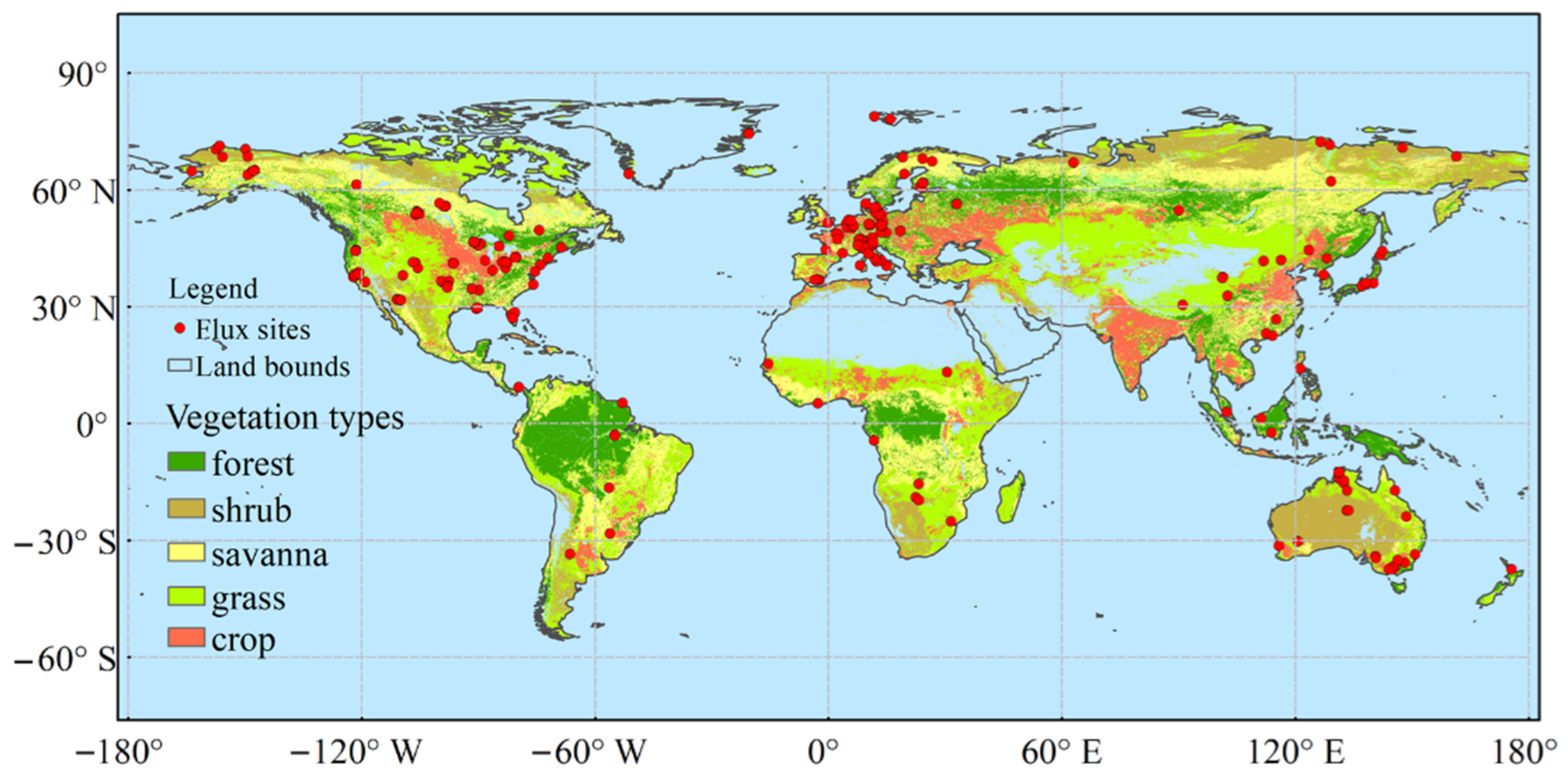
2.1. Data Sources

We used Moderate Resolution Imaging Spectroradiometer (MODIS) datasets, including global Gross Primary Productivity product (MOD17A2H V6) and land cover type products (MCD12Q1 V6), both of which have a spatial resolution of 500 m. MOD17A2H is a dataset containing cumulative 8-day composite and time-series GPP applicable to extracting vegetation phenology (SOS and EOS). This GPP dataset contains a quality control 8-bit band (Psn_QC) to flag poor quality pixels; the first bit with value zero demonstrates good quality. We selected the MODIS datasets from 2001 to 2020. The International Geosphere-Biosphere Programme (IGBP) from MCD12Q1 provides consistent vegetation cover classification schema with many global field observation programs. Particularly, FLUXNET consists of a global network of tower sites that use eddy covariance to measure the exchanges of carbon dioxide, water vapor, and energy between the biosphere and atmosphere [29].

FLUXNET2015 is the latest freely downloadable FLUXNET data (https://fluxnet.org, accessed on 10 August 2022). Compared with its predecessor, the 2007 LaThuile database, the FLUXNET2015 database has been improved in both data quality control and data processing procedures [8]. There are 212 stations worldwide [29]. We selected the data from station sites according to the following criteria. (1) The sites had complete and continuous observations for at least one year, (2) the vegetation type of the site was consistent with the MODIS IGBP type, and (3) quality control was performed (>80% of the sampled data show good quality) [8,30]. The raw observations from the stations have a fine temporal resolution of a half hour/hour. The fine-temporal-scale datasets are aggregated into secondary products with daily, monthly, and annual resolutions. Sample points from the daytime (GPP_DT_VUT_REF) and nighttime (GPP_NT_VUT_REF) methods are available from the FLUXNET2015, but the phenology extracted from either of them was proved to be identical to each other, thus we only applied GPP_NT_VUT_REF to extract the site-based phenology to validate remote-sensing-derived phenological metrics. A detailed description of the process for preparing a good quality station-based dataset has been documented previously [8]. The IGBP land (vegetation) cover types from MCD12Q1 were further reclassified into five groups, including forest(s) (evergreen needleleaf forests, evergreen broadleaf forests, deciduous needleleaf forests, deciduous broadleaf forests, and mixed forests), shrub (open shrublands and closed shrublands), savannas (woody savannas and savannas), grass (grasslands), and crop (croplands and cropland/natural vegetation mosaics). The vegetation cover and the locations of FLUXNET stations are presented in Figure 1.

In addition, monthly average temperature and total precipitation were extracted from the ERA5-Land with a spatial resolution of ~10 km [31]. ERA5-Land was produced by replaying the land component of the ECMWF ERA5 climate reanalysis [32] and made available to facilitate many applications requiring easy and fast access to the data. The dataset is freely available in the Google Earth Engine (GEE) platform and has been applied in many ecological studies [33,34,35]. To make all data have an identical resolution, both temperature (unit °K) and precipitation (in centimeter/month) were resampled to 500 m by bi-cubic interpolation.

2.2. Methodology

The temporal dynamics in vegetation growth can be reflected by the changes in the physiological activity, density, or greenness of vegetation cover. The flux-based GPP data reflect the physiological activity of the underneath vegetation and measure the carbon flux, which can be applied to model the amount of carbon dioxide absorbed through photosynthesis in a unit time. GPP begins to increase significantly with the onset of green-up and decrease rapidly with the onset of dormancy. Thus, the physiological activity reflected by GPP can provide a valuable indicator to estimate the vegetation growth cycle, which can be further used to derive the dates of vegetation phenological events.

Similarly, spatio–temporal GPP dynamics derived from remote sensing technology can be applied to map vegetation phenology over a large area. For any given location, the best curve fit for time-series GPP (usually within a year) contains critical information for one growing cycle of vegetation from which vegetation phenology can be extracted. The inflection point detection method, which locates the dates corresponding to the inflection point in the vegetation GPP curve, was applied to identify the phenological dates for SOS and EOS (Figure 2). Two steps, time-series data preparation and location of phenological dates, were involved. The objective of data preparation was to prepare high-quality data that captured the temporal changes for GPP using smoothing functions (i.e., Savitzky–Golay or SG smoothing), because the original data may inevitably contain noise, which causes abnormal values. The second stage was to locate the phenological dates. The DOY corresponding to the characteristic point in the smoothed curve (e.g., the point of maximum curvature, the point of maximum first-order derivative, or the point of maximum relative change, and so on) is the phenological metrics [36]. Detail processes are listed as below.

2.2.1. Curve Smoothing

The GPP products from remote sensing data, i.e., MOD17A2H, can be affected by clouds, cloud shadows, and snow and ice cover. Before curve smoothing, these poor-quality pixels were removed by the quality control band (Psn_QC band) in the data, and only good-quality pixels were retained. SG smoothing was applied to the GPP data to rectify values that were too high or too low compared with the neighbors [37,38,39], in the form of

$$Y_j^{*}=\frac{{{\displaystyle \sum }}_{i=-m}^{i=m}{C}_i{Y}_{j+i}}{N}$$

(1)

where Y_j+i is the original GPP value of the i + j sample; Y* is the smoothed GPP value; C_i is the coefficient or weight of the ith sample and can be obtained by least square fitting from a polynomial; and N = 2m + 1 is the total sample size in the filtering window, where m is a parameter that determines the size of the moving window.

2.2.2. Fitting and Interpolation

The harmonic analysis has been widely applied to fit time-series data [9,17]. The dynamics of GPP were fit for the smoothed GPP at 8-day intervals using time-series harmonic analysis first. The parameters in the curve fitting are solved by the least squares technique at each individual pixel [40].

$$y\left(t_j\right)=a_0+{\displaystyle \sum }_{i=1}^n\left[a_i\cos \left(2\pi f_i{t}_j\right)+b_{i}sin\left(2\pi f_i{t}_j\right)\right]$$

(2)

where y is the reconstructed series GPP value with 8-day intervals; t_j is the time (day of year, DOY); n is the window size, which is empirically set to 4; f_i is frequency; and a_i and b_i are coefficients to be fit. The GPP time series with an 8-day interval were then expanded to daily resolution through time interpolation.

2.2.3. Phenology Extraction

FOD is the derivative of GPP over time. The dates for SOS and EOS were then extracted from the smoothed GPP curve based on FOD. Specifically, the date corresponding to the maximum and minimum value in FOD of the fitted curve was determined as SOS and EOS, respectively [14,36].

$$\mathrm{FOD}=dGPP/dt$$

(3)

$$\mathrm{SOS}=\mathrm{doy}\{Max{\left(FOD\right)}_{10\%}$$

(4)

$$\mathrm{EOS}=\mathrm{doy}\{Min{\left(FOD\right)}_{10\%}$$

(5)

$$\mathrm{LOS}=\{\begin{array}{c}\mathrm{EOS}-\mathrm{SOS}, \mathrm{if} \mathrm{SOS}\le \mathrm{EOS}\\ \left(\mathrm{EOS}-\mathrm{SOS}\right)+365, \mathrm{if} \mathrm{SOS}>\mathrm{EOS}\end{array}$$

(6)

where dGPP/dt denotes the derivative of GPP against time in DOY; Max and Min are functions to obtain the maximum and minimum values, respectively, from the FOD curves; and doy is defined as the function to locate the dates corresponding to the critical FOD points dependent on the maximum and minimum. For ecosystems showing multiple growing seasons within an annual growth cycle, the critical FOD values are taken to be the first and last FOD points with values less than 10% of the maximum and minimum in relative difference within that cycle. The critical FOD values take the maximum and minimum FOD if all of the other FOD points in an annual vegetation growth cycle present values less than 90% of the maximum or minimum in relative difference.

SOS corresponds to the date observing the most rapid increase in GPP, while EOS is the ending date of the growing season showing the rapid decline in GPP, and LOS is the length of the growing season between SOS and EOS (Figure 2). The MODIS-GPP product is modeled from multiple factors, including meteorological variables such as precipitation and temperature. The FOD-based approach can minimize the direct linkage between the climate factors and the dates of the phenological events and help to reveal the hidden linear correlation, if any, between the climate variables and vegetation phenology. A noticeable difference in the typical FOD curves in the Southern Hemisphere is that the most rapid increase in GPP and thus the maximum FOD is present in the second half of the year, as opposed to that in the first half of the year in the Northern Hemisphere; for both cases, the critical FOD point could be detected by the functions. Unlike the predefined threshold method, this derivative approach has the advantage of calculating the dates dynamically for each pixel based on the unique curve in vegetation photosynthesis over time. Vegetation in evergreen forests and desert areas presented no obvious seasonality [12,22] and was excluded from further analysis. The mean and standard deviation of the phenological events (SOS, EOS, and LOS) over the years of the study period were calculated from the annual distribution of the respective maps.

The remote-sensing-derived phenological events can be validated through the flux-based observations [41]. Similar processes were performed to derive qualified GPP data for the observations. Two metrics, root mean square error (RMSE) and mean error (ME), were used to measure the modeled accuracy and bias for the remotely sensed phenological dates using the flux-based data as the baseline, in the forms of

$$RMSE=\sqrt{\frac{1}{m}{{\displaystyle \sum }}_{i=1}^m{\left(y_{RS}-y_{flux}\right)}^2}$$

(7)

$$ME=\frac{1}{m}{{\displaystyle \sum }}_{i=1}^m\left(y_{RS}-y_{flux}\right)$$

(8)

where m is the sample size and y_RS and y_flux are the SOS and EOS dates obtained from remote sensing and flux-based observation sites, respectively.

2.2.4. Trend Analysis

Trend analysis reveals temporal patterns in phenology, i.e., whether the phenological metrics tend to increase or decrease over the years. This paper applied Sen’s slope to quantify the magnitude of the trend. The significance of the trend is determined by the Mann–Kendall (MK) test. The Sen’s slope analysis does not require the data to obey a particular distribution (e.g., normal distribution) and missing data or the presence of outliers do not significantly affect the results [42]; however, it lacks a statistical significance test for the trends, which can be supplemented by the MK significance test. The MK significance test is suitable for assessing monotonic trends in discrete data, such as SOS, EOS, and LOS [42,43,44]. Pixels with significant trends in SOS, EOS, and LOS were determined by Z scores of the nonparametric Mann–Kendall significance test at a 95% significance level [45]. We further applied a sigma confidence interval to denote the uncertainty associated with the slopes, which is documented in the literature [46,47]. Sen’s slope and the MK test are calculated as follows:

$$slope=median\left(slopes\right)=median\left(\frac{x_j-x_i}{j-i}\right), \forall n>j>i>1$$

(9)

$$sgn\left(x_j-x_i\right)=\{\begin{array}{c}1 ,if x_j-x_i>0\\ 0 , if x_j-x_i=0\\ -1 ,if x_j-x_i<0\end{array}$$

(10)

$$S={{\displaystyle \sum }}_{i=1}^{n-1}{{\displaystyle \sum }}_{j=i+1}^{n}sgn\left(x_j-x_i\right)$$

(11)

$$Var\left(S\right)=\frac{n\left(n-1\right)\left(2n+5\right)+\sum t_i\left(t_i-1\right)\left(2t_i+5\right)}{18}$$

(12)

$$Z=\{\begin{array}{c}S-\frac{1}{\sqrt{Var\left(S\right)}}, S>0\\ 0, S=0\\ S+\frac{1}{\sqrt{Var\left(S\right)}}, S<0\end{array}$$

(13)

where x_j and x_i denote the phenological values at time j and time i, respectively; n denotes the number of data points in the time series; slope denotes the trend of current phenological changes over time; median is the function that calculates the median; slope is the trend of the data variation; sgn denotes the symbolic function; x_j and x_i denote the point pairs in the phenological time-series data; Var(S) denotes the variance of S; and t_i is the number of ties present with i as the extent. Z is the standardized statistics of the dataset. If |Z| > Z_1−α/2, the trend is statistically significant; otherwise, the trend is not statistically significant and, in this paper, this means that the vegetation phenology does not change significantly. The significance level of α was set at 0.05 in this study.

2.2.5. Correlation Analysis

The relationship between meteorological factors (temperature and precipitation) and phenological metrics (SOS, EOS, and LOS) was measured by partial correlation analysis. In addition, to capture any stable temporal lag effect in the relationship between the variables, we aggregated the meteorological variables from the monthly scale to the seasonal scale, as climate variables at the monthly scale can fluctuate considerably. We tested the four seasons, including January–March, April–June, July–September, and October–December. The Pearson correlation takes the form of

$$r_{xy}=\frac{{{\displaystyle \sum }}_{i=1}^n\left(x_i-x_{mean}\right)\left(y_i-y_{mean}\right)}{\sqrt{{{\displaystyle \sum }}_{i=1}^n{\left(x_i-x_{mean}\right)}^2{{\displaystyle \sum }}_{i=1}^n{\left(y_i-y_{mean}\right)}^2}}$$

(14)

where r_xy are Pearson correlation coefficients between two random variables x and y; x_i and y_i are the ith paired value of variables x and y, respectively; and x_mean and y_mean are the mean value of the variables x and y. The variables x and y denote a seasonal climate variable (temperature or precipitation) at the seasonal scale and phenological event (SOS, EOS, or LOS). To exclude other confounding effects from any of the climate variables, partial correlation coefficients between the phenology and each of the meteorological factors were calculated and the maximum/minimum value of the correlation coefficient was obtained for all the seasons, in the form of

$$r_{xy}{.}_z=\frac{\left(r_{xy}-r_{xz}\ast r_{yz}\right)}{\sqrt{1-r_{xz}^2}\ast \sqrt{1-r_{yz}^2}}$$

(15)

where r_xy·z is partial correlation of x and y after eliminating the confounding effect from z and x and z each represent either the temperature or precipitation, respectively.

The changes in vegetation phenology could be attributed to climate changes. At the same time, the shifted phenological dates may impose feedback on the climate through updated vegetation carbon capture from terrestrial ecosystems. We hypothesize that the changes in the dates of the phenological events, particularly the length of the vegetation grow season (LOS), could affect global vegetation productivity. Thus, it is meaningful to explore whether the climate factors could explain any shifts in vegetation phenology and whether the shifts in vegetation phenology were associated with the variations in GPP. We used the pixel-based Pearson correlation coefficient to analyze the relationship be-tween LOS and annual GPP.

3. Results

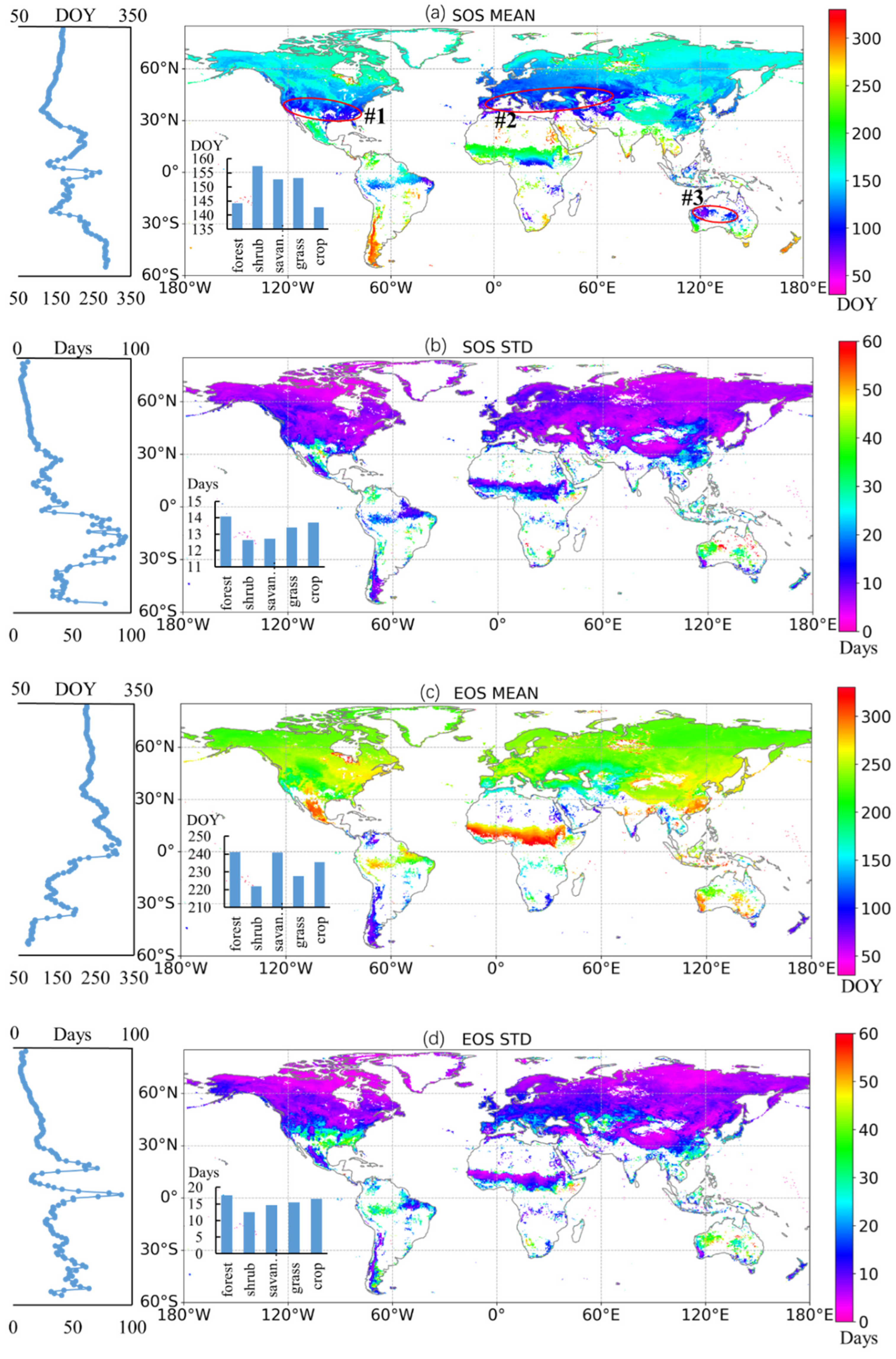
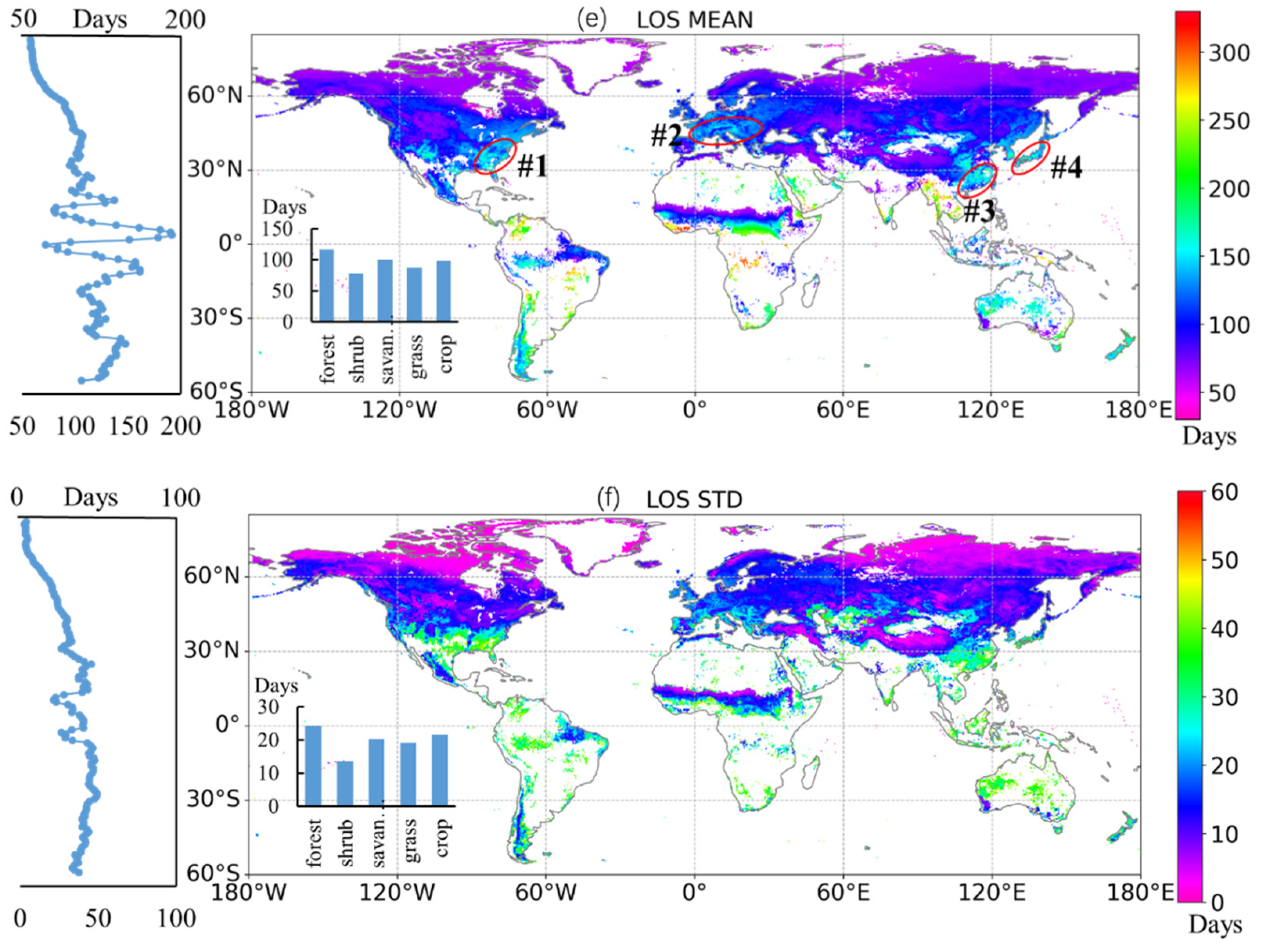
3.1. Spatial Variation in Global Vegetation Phenology

Vegetation phenological metrics modeled from the remote sensing (RS) imagery are generally in agreement with the flux-based observations in terms of RMSE, ME, and the scatter point plots (Figure 3), though disparity exists among the vegetation cover types and phenological events (SOS and EOS) (Figure 3). The RMSE for the modeled SOS and EOS ranges from 10.0 to 37.3 days and 10.4 to 38.1 days, respectively (Figure 3a). The modeled metrics for forest, grass, and croplands show a larger difference from the field observations than those for shrubland and savannas. The statistics of ME indicate that cropland contains the largest overall error in the modeled metrics (Figure 3b). The site–year scatter points between the flux-based observations and remote-sensing-modeled metrics in an annual basis show that they are closely correlated for both SOS and EOS (Figure 3c,d).

The spatial distributions of vegetation phenological events, including SOS, EOS, and LOS, for the temporally averaged mean and standard deviation (std) over the years are shown in Figure 4. The phenological metrics are highly heterogeneous across the study area and vary among the ecosystems. The critical latitudes at 30° in both the Northern Hemisphere and Southern Hemisphere divide the SOS and EOS patterns of the global vegetation into three distinct parts, namely the Northern Hemisphere over 30°N (North), Southern Hemisphere over 30°S (South), and the middle part located between the North and South (Middle). Because of the reversed seasons in the North and the South, SOS in the North starts from March to no later than May (145.72 ± 7.65), while EOS ends after August (243.42 ± 23.95, Figure 4a), but vegetation in the South presents EOS in March, April, or May (126.39 ± 81.22) and SOS after September (269.60 ± 31.02, Figure 4c). Furthermore, SOS varies spatially in the North and the South. Vegetation turns green earlier in a great part of North America (#1) and Southern Europe (#2) compared with that in the rest of the North, and vegetation in Australia (#3) presents earlier green-up than that in the rest of the South (Figure 4a). Both SOS and EOS differ along the latitude belts (Figure 4a,c). For instance, in the North, SOS turns green later along with the northward increase in latitude, while in the South SOS, it is delayed with the southward increase in latitude. EOS advances along the increase in latitude belts in the South, but stays rather stable in the North. The variations in SOS and EOS are reflected by the standard deviation (std) over the years (Figure 4b,d). Both SOS and EOS in the Middle highlight the most sensitive response to the changed latitudes, as shown from the rapid changes in std among the latitude belts. Furthermore, the variation in SOS and EOS is much smaller in the North than that in the South. LOS and its standard deviation (std) computed from the gap between SOS and EOS are shown in Figure 4e,f. Generally, vegetation demonstrates a longer growing season in the South, as shown by the higher LOS in the South (129.86 ± 25.37) than in the North (87.82 ± 45.27). Similarly, LOS near the equator is highly variable along the latitude belts (Figure 4f). In some regions of the Northern Hemisphere, for example, the southeast of the United States (#1), the west of Europe (#2), the south of China (#3), and Japan (#4), where forests are prominent, LOS is rather higher than that in the rest of the North (Figure 4e).

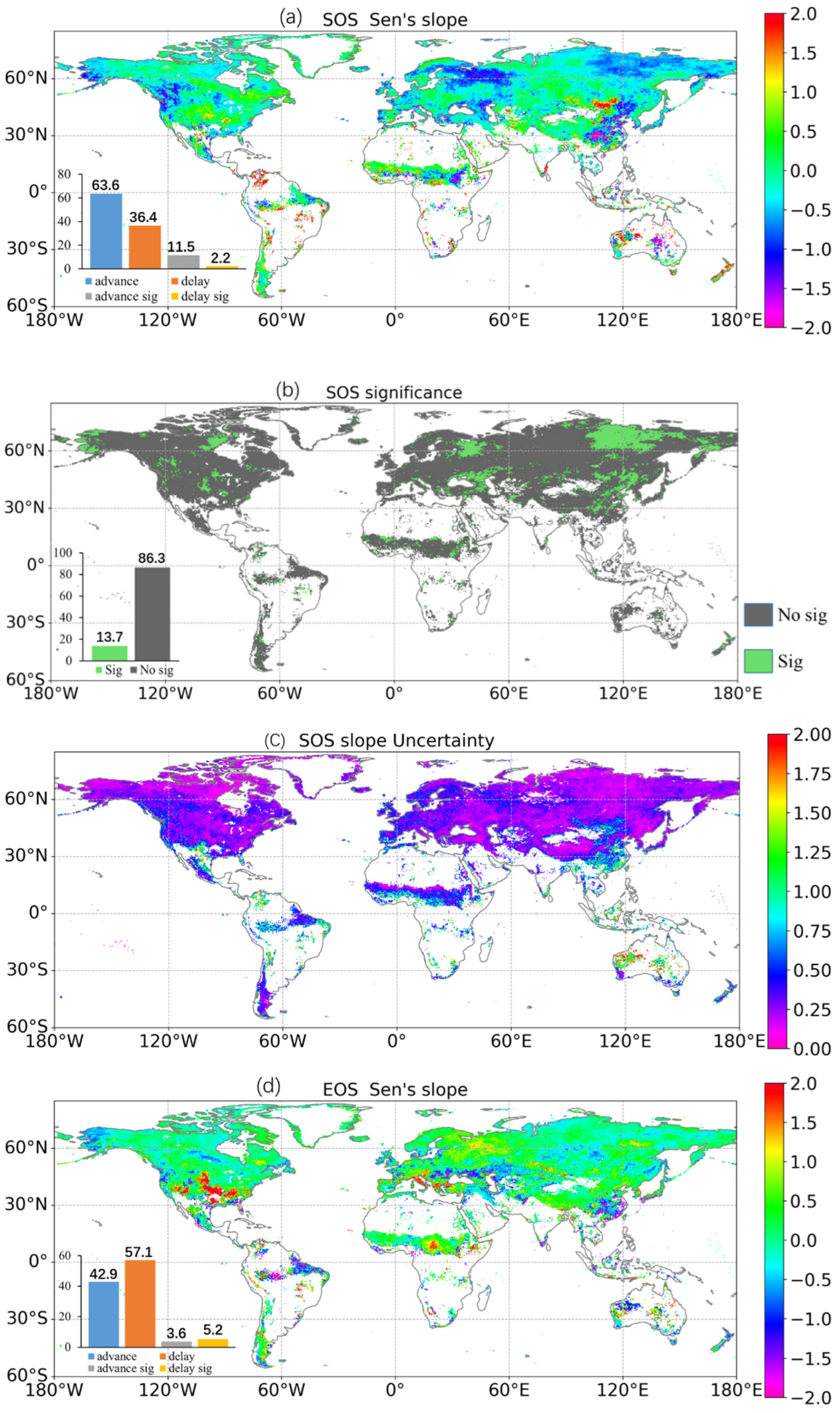
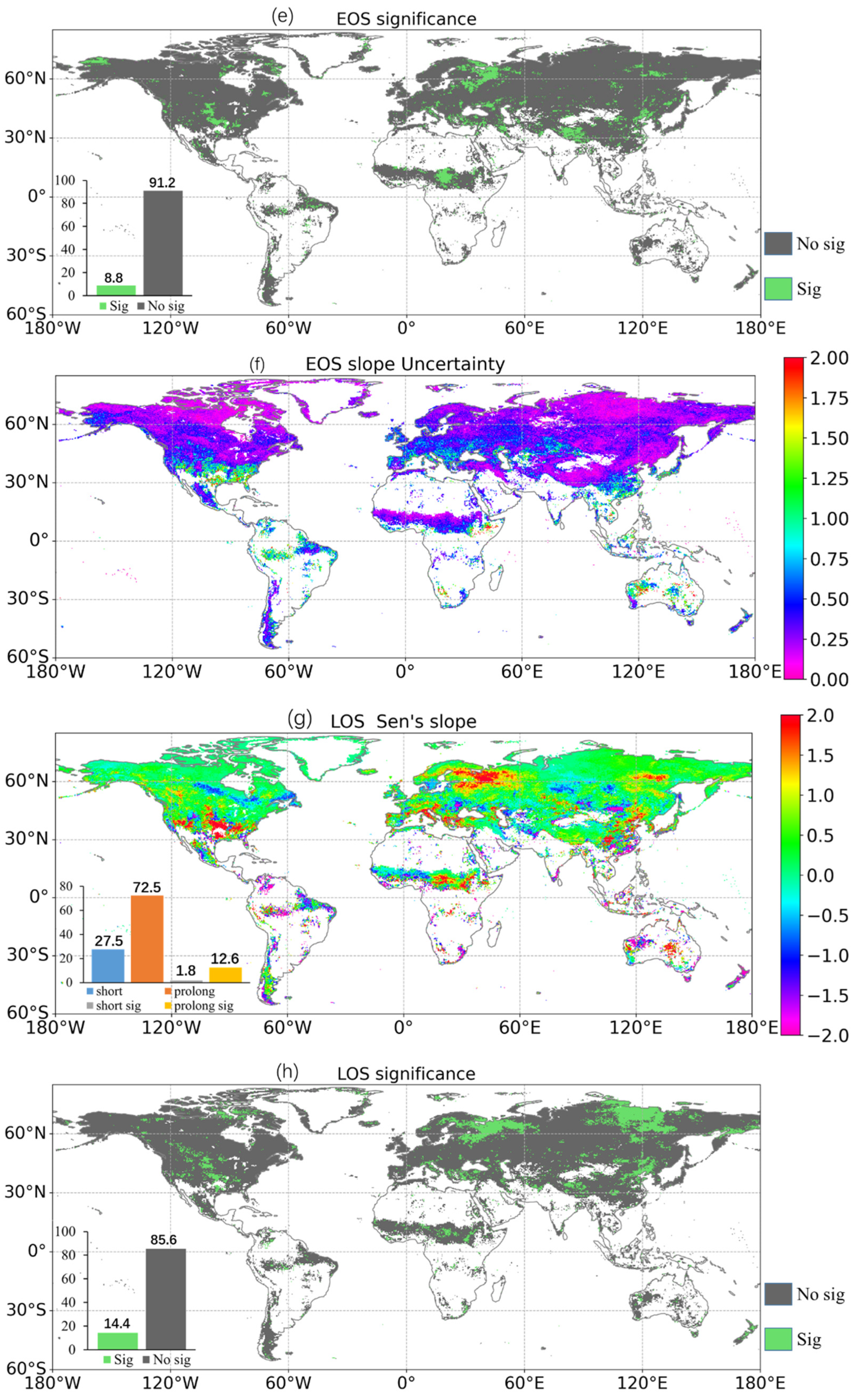
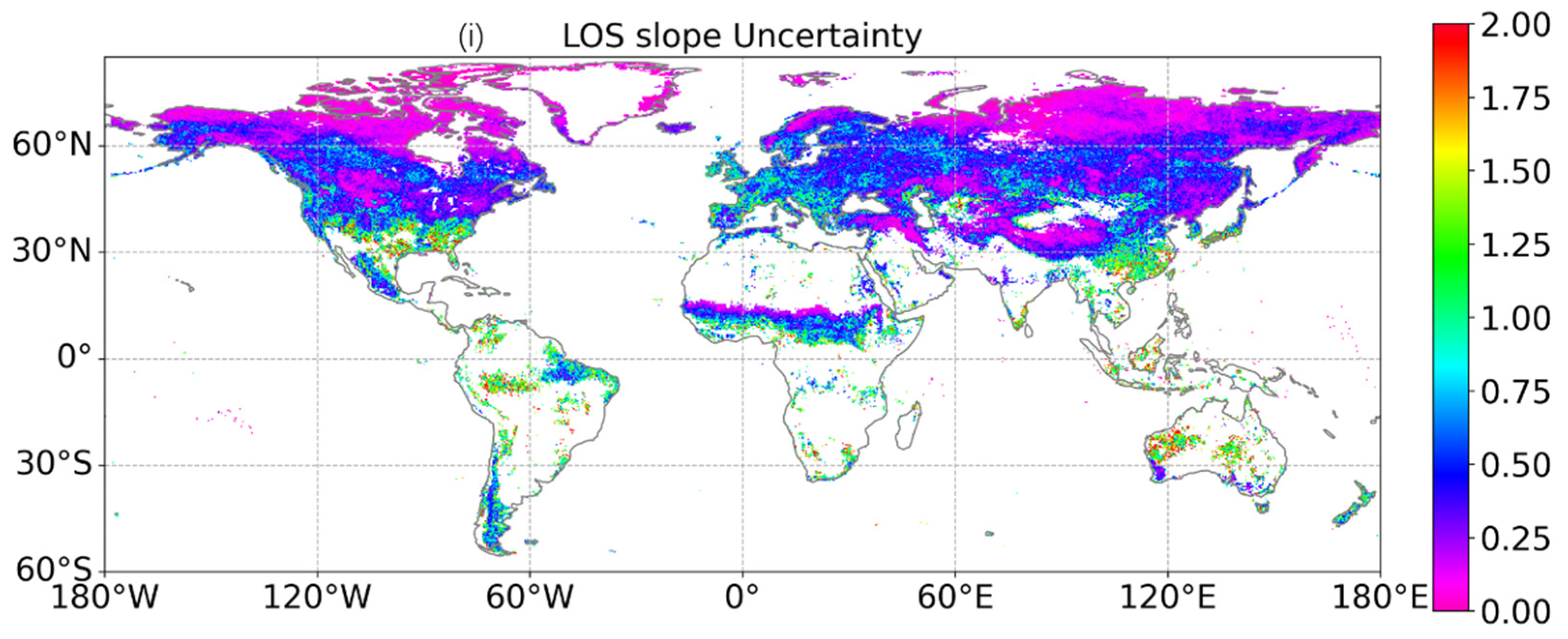
3.2. Temporal Trajectory of the Global Phenological Events

The temporal trends in the phenological events present spatial heterogeneity (Figure 5). SOS advances at an average rate of 0.19 days/year at the global scale, as indicated by the Sen’s slope. Overall, 63.6% of the study area shows advanced SOS, while vegetation green-up in the rest of the area shows a delayed trend over the years. The Mann–Kendall (MK) significant test reveals that the proportion that experienced significant advancement in SOS covers 11.5% of the total area, while it is 2.2% for significantly delayed SOS, notably distributed in the grassland of Inner Mongolia, China, and the northeastern part of Mongolia (Figure 5a,b). EOS is slightly delayed at an average rate of 0.06 days/year (Figure 5c). A larger proportion, or 57.1% of the study area, presents delayed EOS, while the rest experiences earlier EOS, though only 5.2% of the total area is statistically significant in the EOS delay and 3.6% of the vegetated area is significantly advanced in terms of EOS (Figure 5c,d). The updated SOS and EOS results in prolonged LOS, averaging 0.24 days/year at the global scale. The proportion of the area presenting prolonged LOS makes up 72.5% of the total, with only 12.6% being statistically significant (Figure 5e,f). In summary, while advanced SOS and delayed EOS, and thus extended LOS, are observed in a great part of the globally vegetated area, the proportion of the area that passes the significance trend test, including advanced or delayed for SOS and EOS and prolonged or shortened for LOS, is much smaller, covering 13.7%, 8.8%, and 14.4% of the total, respectively.

3.3. Response of the Phenological Events to Climate Changes

The response of SOS to temperature and precipitation is reflected in the correlation analysis (Figures S1–S4) and summarized in Figure 6 and Figure 7. SOS in the Northern Hemisphere predominantly presents a negative correlation with temperature (Figure S1). The distribution of the correlation coefficient between SOS and temperature for different vegetation types appears to be double-peaked. The left side represents areas having a negative correlation and accounts for a much larger part than the right side, which represents a positive correlation between the two variables, indicating that SOS was primarily affected by temperature (Figure 6). The area presenting a negative correlation accounts for 81.2% of all vegetation types (Figure 6f), with the highest being shrub (90.4%, Figure 6e) and the lowest being crop (75.1%, Figure 6a). In the Northern Hemisphere, the shrublands are distributed primarily over 60° in latitude (Figure 1), where the temperature is relatively low. SOS in shrublands might be sensitive to temperature and advanced by a higher temperature. Conversely, croplands are subject to being heavily influenced by anthropogenic activities and the temperature may impose relatively lower impact in most managed croplands. Nevertheless, a significant negative correlation was observed in only half of the area for all vegetation types combined (53.8%, Figure 6e), with the maximum from shrublands (79.0%, Figure 6e) and the minimum from croplands (34.6%, Figure 6a).

The relationship between SOS and precipitation presented a more balanced double-peak pattern (Figures S2 and S7). Besides croplands and shrublands, the other vegetation types exhibit mainly a positive correlation, as reflected from the larger peak of the right side. The proportion showing a positive correlation is 52.3% for the whole study area, which is slightly larger than that showing a negative correlation (47.7%), but the area showing a significant positive correlation is almost double the size of the area showing a significant negative correlation (11.7% vs. 6.4%). Unlike that between SOS and temperature, the area showing a statistically significant correlation between SOS and precipitation, on both the positive and negative side, accounts for a much lower proportion, with the maximum of the positive correlation of savanna taking only 13.2% of the total area.

The response of EOS to the seasonal average temperature and total precipitation presents a similar pattern to that of SOS (Figures S3–S6). A higher temperature is found to possibly induce earlier vegetation dormancy in croplands, grassland, and shrubland, but can delay EOS for most parts of forests and savanna (Figures S3 and S5). Conversely, more precipitation is most likely to postpone EOS for the vegetation types (Figures S4 and S6). Other than the fact that the area showing the highest correlation coefficient between temperature and SOS was found to dominate in the second season (April–July), there was no seasonal difference leading the correlation coefficient between the climate factors and the phenometrics (Figure S7).

3.4. Feedback on GPP from Shifted Vegetation Phenology

The annual global vegetation GPP was on average 595.5 ± 443.5 gC/m²/year during 2001–2020 (Table S1). LOS and annual GPP are positively correlated in ~76% of the study area and significantly positive correlated in ~20% from the correlation analysis (Figure 8). The proportion of area showing a negative correlation between LOS and annual GPP is less than one-third of the total area and is noticeably observed in a part of the Great Plains located in the United States (#1), the south of central Asia (#2), and Inner Mongolia in China and South Mongolia (#3), which are mostly covered by grassland. The relationship between LOS and annual GPP presents a considerable difference in the fraction of the area among the vegetation cover types. The area with LOS and annual GPP positive correlation was much higher than that having a negative correlation for all vegetation types (

Table 1. Proportion of area showing a correlation (and significant correlation) between GPP and LOS.

Item	Forest	Shrub	Savanna	Grass	Crop	All Vegetation
Positive (sig.)	85.1 (29.5)	80.8 (16.6)	83.9 (19.4)	60.4 (12.4)	77.2 (25.4)	75.9 (20.2)
Negative (sig.)	14.9 (0.5)	19.2 (1.1)	16.2 (0.4)	39.6 (5.6)	22.8 (2.3)	24.1 (2.4)

The significance is set at p < 0.05.

). The highest proportion of area with a positive correlation between LOS and annual GPP is found for the forests and the lowest for grasslands, accounting for 85.1% and 60.4% of the total in each class, respectively. The low proportion of grasslands and high proportion of other vegetation cover types may imply that LOS is an important factor for explaining the variance in annual GPP for most vegetated areas.

4. Discussion

4.1. Interactions between Climate Changes and Shifted Vegetation Phenology

Global vegetation phenology was found to correlate with the temperature and precipitation factors. Changes in vegetation phenology may impact vegetation productivity, which in turn can affect carbon sequestration from the atmosphere and have feedback on climate changes. Our study reveals that the rising temperature explains the advanced vegetation green-up for over 80% of the vegetated area, which is generally consistent with other studies in that an increased temperature induced earlier SOS [8,48,49]. Meanwhile, the rising temperature was found to delay SOS in some other regions, most of which are located in the Southern Hemisphere (Figure S1). The climate factors that cause a differentiated response in vegetation phenology might be dependent on the constraint on vegetation growth in local natural environments. For example, a previous study found that vegetation phenology was prominently constrained by precipitation in grasslands in Inner Mongolia, while it was primarily controlled by temperature in grasslands of the Tibetan Plateau [23].

Changes in vegetation phenology interact with vegetation productivity. A positive correlation between GPP and LOS was revealed in our study (Figure 8). A prolonged LOS leads to an increase in GPP, and vice versa (Figure 9). However, we found a proportion of negative correlations in grasslands in some regions between GPP and LOS; a similar finding was reported previously [44,50,51]. We speculate that human activities could be one of the factors leading to the different pattern in grasslands, though extra study is required to confirm this hypothesis. Improving sequestration of the atmospheric carbon dioxide from terrestrial vegetation is believed to be helpful to mitigate climate changes and realize the goal of maintaining global warming under 1.5 °C, in accord with the Paris Agreement [26]. Overall, global warming advances SOS and extends LOS and helps vegetation to sequester more carbon dioxide, which serves positive feedback to counteract global warming.

4.2. Uncertainties in the Retrieved Phenology

Global vegetation phenological events, including SOS, EOS, and LOS, were mapped from remote sensing imagery, with their spatial distribution patterns and trends highlighted in the last two decades. The flux-based observations were used to validate the remote-sensing-derived phenological metrics. We acknowledge that several factors can lead to uncertainties in the extraction of the phenological dates.

First, the fitting models of vegetation photosynthesis level can introduce extra noise in some cases. In this study, the curves of vegetation photosynthesis level were fitted using harmonic functions, which, despite being applied widely, are sensitive to missing data, possibly even resulting in degraded data quality [18,19]. In addition, mapping vegetation phenology at the continental or global scale requires locally adjusted extraction models to provide an accurate result [22]. A number of methods, including the amplitude threshold, first-order derivative (FOD), second-order derivative, relative changing rate, third-order derivative, and curvature change rate, were proposed to retrieve SOS and EOS [14]. Although our approach, using FOD, can largely overcome the limitation of the predefined threshold value and is believed to be able to dynamically fit a wide range of conditions, it is not robust for vegetation cover types that show too slow changes or a flat shape in photosynthesis intensity during a growth cycle. Another difficulty in extracting vegetation phenology is related to multiple growing seasons (MGSs), which needs to be addressed [8,14]. MGSs are particularly prominent in croplands characterized by the rotation of crops. In this study, the dates of the year (DOY) corresponding to the maximum and minimum FOD were taken as the SOS and EOS events for vegetation cover presenting a single growth cycle. Additionally, a flexible range of 10% relative difference was used to determine the first and last FOD points if the values were within that range for MGS cases. Nevertheless, the hard-coded threshold of 10% is likely unable to fully address the issue. Both flat-shaped and MGS patterns in vegetation growth cycles are interesting topics that deserve more attention in future studies.

Second, a single indicator, i.e., GPP, might not be sensitive enough to indicate the changes in vegetation phenology. Multiple indicators sensitive to reflect the changes in vegetation at different growth stages may be combined to better reflect the changes in vegetation growth stages. One of the indicators is the optimized soil-adjusted vegetation index (OSAVI), which was found to be a strong predictor of EOS for evergreen needleleaf forests [52]. Solar-induced chlorophyll fluorescence and vegetation optical depth may provide alternative methods to extract vegetation phenology [53,54,55]. Our study provides high-level statistics of the correlations between different ecosystem types, such as croplands, forests, grasslands, savanna, and shrub, and climate variables (Table 1), which is useful to understand the response of vegetation phenology to climate changes for different ecosystems. However, such statistics may not reveal detailed differences within each type.

Lastly, the relatively coarse datasets applied for global-scale vegetation phenology mapping may introduce noise into the final results. The spatial resolution of MODIS data (500 m) is likely to hide the spatial detail in the patterns of vegetation phenology. Spatial resolution is an important factor in phenology extraction, and spatially aggregated GPP over a large area, i.e., 500 m × 500 m, represented by a single pixel can easily smooth out finer location-dependent GPP across an area [56]. The coarse spatial resolution of MODIS data also leads to difficulty in the validation from field-based observations. Similarly, the low-resolution climate datasets might introduce uncertainties in the correlation analysis between the shifted vegetation phenological dates and the climate factors. However, given the global-scale study, the datasets selected in this study are among the best possible candidates that can be applied to analyze the trend in their relationships in the long-term at the global scale. Better downscaling methods and finer data would enhance the reliability of the study results.

5. Conclusions

The global vegetation phenology, including SOS, EOS, and LOS, was mapped using first-order derivative analysis on satellite remotely sensed images for the past two decades. SOS exhibited a significant early trend in 11.5% of the total area, at a rate 0.19 days/year at the global scale, and EOS presented a significant trend of delay in 5.2% of the global vegetated area, which together significantly extended LOS in 12.6% of the vegetated area. This study illustrated the variations in the spatio–temporal dynamics in the vegetation phenology among vegetation cover types and regions across the globe (SM).

This study revealed interactions between vegetation phenology and climate changes. Both temperature and precipitation affect vegetation phenology. A higher temperature as a direct consequence of global warming advanced the vegetation green-up date. On the other hand, 75.9% and 20.2% of the vegetated area showed a positive correlation and significantly positive correlation between annual GPP and length of vegetation growing season (LOS), likely indicating an enhancing effect on vegetation productivity, and thus increased carbon uptake from the shifted vegetation phenology. Our study provides a comprehensive view on the changes in vegetation phenology of global terrestrial ecosystems during the last two decades. The interactions between the shifted vegetation phenology and climate changes may provide useful information for better understanding of the future trajectory of global climate changes.

References

1. Piao, S.; Fang, J.; Zhou, L.; Ciais, P.; Zhu, B. Variations in Satellite-Derived Phenology in China’s Temperate Vegetation. Glob. Chang. Biol. 2006, 12, 672–685. [Google Scholar] [CrossRef]
2. Xie, Q.; Cleverly, J.; Moore, C.E.; Ding, Y.; Hall, C.C.; Ma, X.; Brown, L.A.; Wang, C.; Beringer, J.; Prober, S.M.; et al. Land Surface Phenology Retrievals for Arid and Semi-Arid Ecosystems. ISPRS J. Photogramm. Remote Sens. 2022, 185, 129–145. [Google Scholar] [CrossRef]
3. Zhao, G.; Gao, Y.; Gao, S.; Xu, Y.; Liu, J.; Sun, C.; Gao, Y.; Liu, S.; Chen, Z.; Jia, L. The Phenological Growth Stages of Sapindus Mukorossi According to BBCH Scale. Forests 2019, 10, 462. [Google Scholar] [CrossRef] [Green Version]
4. Cleland, E.E.; Chuine, I.; Menzel, A.; Mooney, H.A.; Schwartz, M.D. Shifting Plant Phenology in Response to Global Change. Trends Ecol. Evol. 2007, 22, 357–365. [Google Scholar] [CrossRef] [PubMed]
5. Caparros-Santiago, J.A.; Rodriguez-Galiano, V.; Dash, J. Land Surface Phenology as Indicator of Global Terrestrial Ecosystem Dynamics: A Systematic Review. ISPRS J. Photogramm. Remote Sens. 2021, 171, 330–347. [Google Scholar] [CrossRef]
6. Peng, D.; Wu, C.; Li, C.; Zhang, X.; Liu, Z.; Ye, H.; Luo, S.; Liu, X.; Hu, Y.; Fang, B. Spring Green-up Phenology Products Derived from MODIS NDVI and EVI: Intercomparison, Interpretation and Validation Using National Phenology Network and AmeriFlux Observations. Ecol. Indic. 2017, 77, 323–336. [Google Scholar] [CrossRef]
7. Aires, L.M.I.; Pio, C.A.; Pereira, J.S. Carbon Dioxide Exchange above a Mediterranean C3/C4 Grassland during Two Climatologically Contrasting Years. Glob. Chang. Biol. 2008, 14, 539–555. [Google Scholar] [CrossRef] [Green Version]
8. Wang, X.; Xiao, J.; Li, X.; Cheng, G.; Ma, M.; Zhu, G.; Altaf Arain, M.; Andrew Black, T.; Jassal, R.S. No Trends in Spring and Autumn Phenology during the Global Warming Hiatus. Nat. Commun. 2019, 10, 2389. [Google Scholar] [CrossRef] [PubMed] [Green Version]
9. White, M.A.; de Beurs, K.M.; Didan, K.; Inouye, D.W.; Richardson, A.D.; Jensen, O.P.; O’Keefe, J.; Zhang, G.; Nemani, R.R.; van Leeuwen, W.J.D.; et al. Intercomparison, Interpretation, and Assessment of Spring Phenology in North America Estimated from Remote Sensing for 1982–2006. Glob. Chang. Biol. 2009, 15, 2335–2359. [Google Scholar] [CrossRef]
10. Kaspar, F.; Zimmermann, K.; Polte-Rudolf, C. An Overview of the Phenological Observation Network and the Phenological Database of Germany’s National Meteorological Service (Deutscher Wetterdienst). Adv. Sci. Res. 2015, 11, 93–99. [Google Scholar] [CrossRef] [Green Version]
11. Donnelly, A.; Yu, R.; Jones, K.; Belitz, M.; Li, B.; Duffy, K.; Zhang, X.; Wang, J.; Seyednasrollah, B.; Gerst, K.L.; et al. Exploring Discrepancies between in Situ Phenology and Remotely Derived Phenometrics at NEON Sites. Ecosphere 2022, 13, e3912. [Google Scholar] [CrossRef]
12. Zhang, X.; Friedl, M.A.; Schaaf, C.B. Global Vegetation Phenology from Moderate Resolution Imaging Spectroradiometer (MODIS): Evaluation of Global Patterns and Comparison with in Situ Measurements. J. Geophys. Res. Biogeosci. 2006, 111, 1–14. [Google Scholar] [CrossRef]
13. Fisher, J.I.; Mustard, J.F.; Vadeboncoeur, M.A. Green Leaf Phenology at Landsat Resolution: Scaling from the Field to the Satellite. Remote Sens. Environ. 2006, 100, 265–279. [Google Scholar] [CrossRef]
14. Wu, W.; Sun, Y.; Xiao, K.; Xin, Q. Development of a Global Annual Land Surface Phenology Dataset for 1982–2018 from the AVHRR Data by Implementing Multiple Phenology Retrieving Methods. Int. J. Appl. Earth Obs. Geoinf. 2021, 103, 102487. [Google Scholar] [CrossRef]
15. Xu, C.; McDowell, N.G.; Fisher, R.A.; Wei, L.; Sevanto, S.; Christoffersen, B.O.; Weng, E.; Middleton, R.S. Increasing Impacts of Extreme Droughts on Vegetation Productivity under Climate Change. Nat. Clim. Chang. 2019, 9, 948–953. [Google Scholar] [CrossRef] [Green Version]
16. Fang, J.; Li, X.; Xiao, J.; Yan, X.; Li, B.; Liu, F. Vegetation Photosynthetic Phenology Metrics in Northern Terrestrial Ecosystems: A Dataset Derived from a Gross Primary Productivity Product Based on Solar-Induced Chlorophyll Fluorescence. Earth Syst. Sci. Data 2022, 107, 1590–1598. [Google Scholar] [CrossRef]
17. Cong, N.; Piao, S.; Chen, A.; Wang, X.; Lin, X.; Chen, S.; Han, S.; Zhou, G.; Zhang, X. Spring Vegetation Green-up Date in China Inferred from SPOT NDVI Data: A Multiple Model Analysis. Agric. For. Meteorol. 2012, 165, 104–113. [Google Scholar] [CrossRef]
18. Cong, N.; Wang, T.; Nan, H.; Ma, Y.; Wang, X.; Myneni, R.B.; Piao, S. Changes in Satellite-Derived Spring Vegetation Green-up Date and Its Linkage to Climate in China from 1982 to 2010: A Multimethod Analysis. Glob. Chang. Biol. 2013, 19, 881–891. [Google Scholar] [CrossRef]
19. Hansen, J.; Sato, M.; Ruedy, R.; Lo, K.; Lea, D.W.; Medina-Elizade, M. Global Temperature Change. Proc. Natl. Acad. Sci. USA 2006, 103, 14288–14293. [Google Scholar] [CrossRef] [Green Version]
20. Shen, M.; Wang, S.; Jiang, N.; Sun, J.; Cao, R.; Ling, X.; Fang, B.; Zhang, L.; Zhang, L.; Xu, X.; et al. Plant Phenology Changes and Drivers on the Qinghai–Tibetan Plateau. Nat. Rev. Earth Environ. 2022, 3, 633–651. [Google Scholar] [CrossRef]
21. Sha, Z.; Zhong, J.; Bai, Y.; Tan, X.; Li, J. Spatio-Temporal Patterns of Satellite-Derived Grassland Vegetation Phenology from 1998 to 2012 in Inner Mongolia, China. J. Arid Land 2016, 8, 462–477. [Google Scholar] [CrossRef] [Green Version]
22. Wang, L.; Tian, F.; Wang, Y.; Wu, Z.; Schurgers, G.; Fensholt, R. Acceleration of Global Vegetation Greenup from Combined Effects of Climate Change and Human Land Management. Glob. Chang. Biol. 2018, 24, 5484–5499. [Google Scholar] [CrossRef] [PubMed]
23. Liu, Q.; Fu, Y.H.; Zeng, Z.; Huang, M.; Li, X.; Piao, S. Temperature, Precipitation, and Insolation Effects on Autumn Vegetation Phenology in Temperate China. Glob. Chang. Biol. 2016, 22, 644–655. [Google Scholar] [CrossRef] [PubMed]
24. Piao, S.; Fang, J.; Zhou, L.; Zhu, B.; Tan, K.; Tao, S. Changes in Vegetation Net Primary Productivity from 1982 to 1999 in China. Global Biogeochem. Cycles 2005, 19, 1–16. [Google Scholar] [CrossRef] [Green Version]
25. White, M.A.; Running, S.W.; Thornton, P.E. The Impact of Growing-Season Length Variability on Carbon Assimilation and Evapotranspiration over 88 Years in the Eastern US Deciduous Forest. Int. J. Biometeorol. 1999, 42, 139–145. [Google Scholar] [CrossRef] [PubMed]
26. Wei, Y.M.; Han, R.; Wang, C.; Yu, B.; Liang, Q.M.; Yuan, X.C.; Chang, J.; Zhao, Q.; Liao, H.; Tang, B.; et al. Self-Preservation Strategy for Approaching Global Warming Targets in the Post-Paris Agreement Era. Nat. Commun. 2020, 11, 1624. [Google Scholar] [CrossRef] [PubMed] [Green Version]
27. Wu, C.; Chen, J.M.; Black, T.A.; Price, D.T.; Kurz, W.A.; Desai, A.R.; Gonsamo, A.; Jassal, R.S.; Gough, C.M.; Bohrer, G.; et al. Interannual Variability of Net Ecosystem Productivity in Forests Is Explained by Carbon Flux Phenology in Autumn. Glob. Ecol. Biogeogr. 2013, 22, 994–1006. [Google Scholar] [CrossRef]
28. Fang, J.; Lutz, J.A.; Wang, L.; Shugart, H.H.; Yan, X. Using Climate-Driven Leaf Phenology and Growth to Improve Predictions of Gross Primary Productivity in North American Forests. Glob. Chang. Biol. 2020, 26, 6974–6988. [Google Scholar] [CrossRef]
29. Pastorello, G.; Trotta, C.; Canfora, E.; Chu, H.; Christianson, D.; Cheah, Y.W.; Poindexter, C.; Chen, J.; Elbashandy, A.; Humphrey, M.; et al. The FLUXNET2015 Dataset and the ONEFlux Processing Pipeline for Eddy Covariance Data. Sci. Data 2020, 7, 225. [Google Scholar] [CrossRef]
30. Wu, C.; Peng, D.; Soudani, K.; Siebicke, L.; Gough, C.M.; Arain, M.A.; Bohrer, G.; Lafleur, P.M.; Peichl, M.; Gonsamo, A.; et al. Land Surface Phenology Derived from Normalized Difference Vegetation Index (NDVI) at Global FLUXNET Sites. Agric. For. Meteorol. 2017, 233, 171–182. [Google Scholar] [CrossRef]
31. Li, H.; Liu, G.; Han, C.; Yang, Y.; Chen, R. Quantifying the Trends and Variations in the Frost-Free Period and the Number of Frost Days across China under Climate Change Using ERA5-Land Reanalysis Dataset. Remote Sens. 2022, 14, 2400. [Google Scholar] [CrossRef]
32. Vanella, D.; Longo-Minnolo, G.; Belfiore, O.R.; Ramírez-Cuesta, J.M.; Pappalardo, S.; Consoli, S.; D’Urso, G.; Chirico, G.B.; Coppola, A.; Comegna, A.; et al. Comparing the Use of ERA5 Reanalysis Dataset and Ground-Based Agrometeorological Data under Different Climates and Topography in Italy. J. Hydrol. Reg. Stud. 2022, 42, 101182. [Google Scholar] [CrossRef]
33. Stefanidis, K.; Varlas, G.; Vourka, A.; Papadopoulos, A.; Dimitriou, E. Delineating the Relative Contribution of Climate Related Variables to Chlorophyll-a and Phytoplankton Biomass in Lakes Using the ERA5-Land Climate Reanalysis Data. Water Res. 2021, 196, 117053. [Google Scholar] [CrossRef] [PubMed]
34. Liu, J.; Hagan, D.F.T.; Liu, Y. Global Land Surface Temperature Change (2003–2017) and Its Relationship with Climate Drivers: Airs, Modis, and Era5-Land Based Analysis. Remote Sens. 2021, 13, 44. [Google Scholar] [CrossRef]
35. Chinita, M.J.; Richardson, M.; Teixeira, J.; Miranda, P.M.A. Global Mean Frequency Increases of Daily and Sub-Daily Heavy Precipitation in ERA5. Environ. Res. Lett. 2021, 16, 074035. [Google Scholar] [CrossRef]
36. Xin, Q.; Li, J.; Li, Z.; Li, Y.; Zhou, X. Evaluations and Comparisons of Rule-Based and Machine-Learning-Based Methods to Retrieve Satellite-Based Vegetation Phenology Using MODIS and USA National Phenology Network Data. Int. J. Appl. Earth Obs. Geoinf. 2020, 93, 102189. [Google Scholar] [CrossRef]
37. Cai, Z.; Jönsson, P.; Jin, H.; Eklundh, L. Performance of Smoothing Methods for Reconstructing NDVI Time-Series and Estimating Vegetation Phenology from MODIS Data. Remote Sens. 2017, 9, 1271. [Google Scholar] [CrossRef] [Green Version]
38. Fan, D.; Zhu, W.; Pan, Y.; Jiang, N. Noise Detection for NDVI Time Series Based on Dixon’s Test and Application in Data Reconstruction. J. Remote Sens. 2013, 17, 1158–1174. [Google Scholar]
39. Chen, J.; Jönsson, P.; Tamura, M.; Gu, Z.; Matsushita, B.; Eklundh, L. A Simple Method for Reconstructing a High-Quality NDVI Time-Series Data Set Based on the Savitzky—Golay Filter. Remote Sens. Environ. 2004, 91, 332–344. [Google Scholar] [CrossRef]
40. Zhou, J.; Jia, L.; Menenti, M. Reconstruction of Global MODIS NDVI Time Series: Performance of Harmonic ANalysis of Time Series (HANTS). Remote Sens. Environ. 2015, 163, 217–228. [Google Scholar] [CrossRef]
41. Gray, R.E.J.; Ewers, R.M. Monitoring Forest Phenology in a Changing World. Forests 2021, 12, 297. [Google Scholar] [CrossRef]
42. Sun, H.; Wang, J.; Xiong, J.; Bian, J.; Jin, H.; Cheng, W.; Li, A. Vegetation Change and Its Response to Climate Change in Yunnan Province, China. Adv. Meteorol. 2021, 2021, 1–20. [Google Scholar] [CrossRef]
43. de Jong, R.; de Bruin, S.; de Wit, A.; Schaepman, M.E.; Dent, D.L. Analysis of Monotonic Greening and Browning Trends from Global NDVI Time-Series. Remote Sens. Environ. 2011, 115, 692–702. [Google Scholar] [CrossRef] [Green Version]
44. Sun, H.; Chen, Y.; Xiong, J.; Ye, C.; Yong, Z.; Wang, Y.; He, D.; Xu, S. Relationships between Climate Change, Phenology, Edaphic Factors, and Net Primary Productivity across the Tibetan Plateau. Int. J. Appl. Earth Obs. Geoinf. 2022, 107, 102708. [Google Scholar] [CrossRef]
45. Eastman, J.R.; Sangermano, F.; Ghimire, B.; Zhu, H.; Chen, H.; Neeti, N.; Cai, Y.; Machado, E.A.; Crema, S.C. Seasonal Trend Analysis of Image Time Series. Int. J. Remote Sens. 2009, 30, 2721–2726. [Google Scholar] [CrossRef]
46. Sen, P.K. Estimates of the Regression Coefficient Based on Kendall’s Tau. J. Am. Stat. Assoc. 1968, 63, 1379–1389. [Google Scholar] [CrossRef]
47. Bulgin, C.E.; Merchant, C.J.; Ferreira, D. Tendencies, Variability and Persistence of Sea Surface Temperature Anomalies. Sci. Rep. 2020, 10, 7986. [Google Scholar] [CrossRef]
48. Yang, B.; He, M.; Shishov, V.; Tychkov, I.; Vaganov, E.; Rossi, S. New Perspective on Spring Vegetation Phenology and Global Climate Change Based on Tibetan Plateau Tree-Ring Data. Proc. Natl. Acad. Sci. USA 2017, 114, 6966–6971. [Google Scholar] [CrossRef] [Green Version]
49. Vitasse, Y.; Delzon, S.; Dufrêne, E.; Pontailler, J.Y.; Louvet, J.M.; Kremer, A.; Michalet, R. Leaf Phenology Sensitivity to Temperature in European Trees: Do within-Species Populations Exhibit Similar Responses? Agric. For. Meteorol. 2009, 149, 735–744. [Google Scholar] [CrossRef]
50. Wu, L.; Ma, X.; Dou, X.; Zhu, J.; Zhao, C. Impacts of Climate Change on Vegetation Phenology and Net Primary Productivity in Arid Central Asia. Sci. Total Environ. 2021, 796, 149055. [Google Scholar] [CrossRef]
51. Qiu, Y.; Zhang, L.; Fan, D. Spatio-Temporal Changes of Net Primary Productivity and Its Response to Phenology in Northeast China during 2000–2015. Int. Arch. Photogramm. Remote Sens. Spat. Inf. Sci.-ISPRS Arch. 2018, 42, 1453–1459. [Google Scholar] [CrossRef] [Green Version]
52. Wu, C.; Gonsamo, A.; Gough, C.M.; Chen, J.M.; Xu, S. Modeling Growing Season Phenology in North American Forests Using Seasonal Mean Vegetation Indices from MODIS. Remote Sens. Environ. 2014, 147, 79–88. [Google Scholar] [CrossRef]
53. Joiner, J.; Yoshida, Y.; Vasilkov, A.P.; Schaefer, K.; Jung, M.; Guanter, L.; Zhang, Y.; Garrity, S.; Middleton, E.M.; Huemmrich, K.F.; et al. The Seasonal Cycle of Satellite Chlorophyll Fluorescence Observations and Its Relationship to Vegetation Phenology and Ecosystem Atmosphere Carbon Exchange. Remote Sens. Environ. 2014, 152, 375–391. [Google Scholar] [CrossRef] [Green Version]
54. Jones, M.O.; Jones, L.A.; Kimball, J.S.; McDonald, K.C. Satellite Passive Microwave Remote Sensing for Monitoring Global Land Surface Phenology. Remote Sens. Environ. 2011, 115, 1102–1114. [Google Scholar] [CrossRef]
55. Jones, M.O.; Kimball, J.S.; Nemani, R.R. Asynchronous Amazon Forest Canopy Phenology Indicates Adaptation to Both Water and Light Availability. Environ. Res. Lett. 2014, 9, 124021. [Google Scholar] [CrossRef]
56. Peng, D.; Zhang, X.; Zhang, B.; Liu, L.; Liu, X.; Huete, A.R.; Huang, W.; Wang, S.; Luo, S.; Zhang, X.; et al. Scaling Effects on Spring Phenology Detections from MODIS Data at Multiple Spatial Resolutions over the Contiguous United States. ISPRS J. Photogramm. Remote Sens. 2017, 132, 185–198. [Google Scholar] [CrossRef]
Figure 1. Global distribution of vegetation types and locations of FLUXNET (Flux) sites, where land cover type products from MCD12Q1 are reclassified into five groups, including forest(s) (evergreen needleleaf forests, evergreen broadleaf forests, deciduous needleleaf forests, deciduous broadleaf forests, and mixed forests), shrub (open shrublands and closed shrublands), savannas (woody savannas and savannas), grass (grasslands), and crop (croplands and cropland/natural vegetation mosaics).
Remotesensing 15 02288 g001
Figure 2. Typical curve fitting for GPP and vegetation phenology extraction from remotely sensed imagery in the Northern Hemisphere. (a) Time-series remotely-sensed imageries showing time-series changes in vegetation photosynthesis levels, (b) vegetation growth status (GPP) for pixel Pi, (c) smoothed curve, and (d) extracted phenological dates using FOD.
Remotesensing 15 02288 g002
Figure 3. Validation of the remote-sensing-derived phenological metrics, on a yearly basis, against the FLUXNET observations through indicators of (a) root mean square error (RMSE), (b) mean error (ME), (c) scatter of SOS, and (d) scatter of EOS.
Remotesensing 15 02288 g003aRemotesensing 15 02288 g003b
Figure 4. Mean and standard deviation (std) for SOS, EOS, and LOS during 2001–2020, with the mean value aggregated along the latitude gradients at intervals of one degree (see left inset figures). Areas with a lack of data or/and low reliability (no/low obvious seasonality, std ≥ 60 days) are masked out. The critical latitudes at 30° in both the Northern Hemisphere and Southern Hemisphere segment the global vegetation into three distinct parts, the north sector over 30°N northward (North), the south sector over 30°S southward (South), and the middle between them (Middle). Some hotspot regions are labeled, including the southern part of North America, Southern Europe, and Australia in sub-figure (ad), as well as southeast of the United States, west of Europe, south of China, and Japan in sub-figure (ef).
Remotesensing 15 02288 g004aRemotesensing 15 02288 g004b
Figure 5. Trend analysis for the vegetation phenological events during 2001–2020, with the inset figure showing the statistics (percentage of area) from the Sen’s slope trend analysis on the phenological metrics (SOS, EOS, and LOS) as advance/delay and significant advance/delay (advance sig and delay sig) in (a,d), grow season length shortened (short) or prolonged (prolong) and significantly shortened/prolonged (short sig and prolong sig) in (g), and MK significance test on the Sen’s slope (at the probability level of 0.05) with labels’ significance (Sig) and no significance (No sig) in (b,e,h). The spatially averaged values are 0.19, 0.06, and 0.24 days/year for SOS (a), EOS (d), and LOS (g), respectively. Uncertainties reflected by one sigma confidence interval in the trend are given in (c,f,i).
Remotesensing 15 02288 g005aRemotesensing 15 02288 g005bRemotesensing 15 02288 g005c
Figure 6. Double-peak patterns in the histogram of the correlation coefficient between SOS and temperature for different vegetation types and all types combined, with the statistics (percentage of area) for positive (pos) and negative (neg) correlation (and significant correlation) (af). The x-axis was divided into 200 bins for the correlation coefficient located between −1 and 0 (negative correlation) and 0 to 1 (positive correlation), and the y-axis shows the percentage of the count within each bin.
Remotesensing 15 02288 g006
Figure 7. Double-peak patterns in the histogram of the correlation coefficient between EOS and temperature for different vegetation types and all types combined, with the statistics (percentage of area) for positive (pos) and negative (neg) correlation (and significant correlation) (af). The x-axis was divided into 200 bins for the correlation coefficient located between −1 and 0 (negative correlation), and 0 to 1 (positive correlation), and the y-axis shows the percentage of the count within each bin.
Remotesensing 15 02288 g007aRemotesensing 15 02288 g007b
Figure 8. Correlation coefficient between GPP and LOG, with the inset figure showing the proportion of the statistics (percentage of area) for positive (pos) and negative (neg) correlation and significant correlation (pos/neg sig). The labeled numbers in the figure, #1 for the Midwest of the United States, #2 for the south of central Asia, and #3 for Inner Mongolia in China and South Mongolia, exemplify three key regions showing a significantly negative correlation between LOS and GPP.
Remotesensing 15 02288 g008
Figure 9. Comparison of the temporal trends of annual GPP and LOS for the significant positive correlation area, which accounts for 20.2% of the total vegetated area (see Table 1).
Remotesensing 15 02288 g009