Article

Applying Time-Expended Sampling to Ensemble Assimilation of Remote-Sensing Data for Short-Term Predictions of Thunderstorms

1
Institute of Atmospheric Physics, Chinese Academy of Sciences, Beijing 100029, China
2
Cooperative Institute for Severe and High-Impact Weather Research and Operations, University of Oklahoma, Norman, OK 73072, USA
3
University of Chinese Academy of Sciences, Beijing 100029, China
4
NOAA/OAR/National Severe Storms Laboratory (NSSL), Norman, OK 73072, USA
*
Author to whom correspondence should be addressed.
Remote Sens. 2023, 15(9), 2358; https://doi.org/10.3390/rs15092358
Submission received: 20 March 2023 / Revised: 20 April 2023 / Accepted: 26 April 2023 / Published: 29 April 2023

Abstract

:
By sampling perturbed state vectors from each ensemble forecast at additional time levels shifted by ±τ (where τ is a selected time interval) from the analysis time, time-expanded sampling (TES) can not only sample timing errors (or phase errors) but also triple the analysis ensemble size for covariance construction without increasing the forecast ensemble size. In this study, TES was applied to the convection-allowing ensemble-based warn-on-forecast system (WoFS), for four severe storm events, to reduce the computational costs that constrain real-time applications in the assimilation of remote-sensing data from radars and the geostationary satellite GOES-16. For each event, TES was implemented against a 36-member control experiment (E36) by reducing the forecast ensemble size to 12 but tripling the analysis ensemble size to 12 × 3 = 36 with τ = 2.5 min, 5 min and 7.5 min in three TES experiments, named E12×3τ2.5, E12×3τ5 and E12×3τ7.5, respectively. A 0–6-h forecast was created hourly after the second hour during the assimilation in each experiment. The assimilation statistics were evaluated for each experiment applied to each event and were found to be little affected by the TES, while reducing the computational cost. The forecasts produced in each experiment were verified against multi-sensor observed/estimated rainfall, reported tornadoes and damaging winds for each event. The verifications indicated that the forecasts produced in the three TES experiments had about the same capability and quality as that in the E36 for predicting hourly rainfall and the probabilities of tornadoes and damaging winds; in addition, the predictive capability and quality were not sensitive to τ, although they were slightly enhanced by selecting τ = 7.5 min. These results suggest that TES is attractive and useful for cost-saving real-time applications of WoFS in the assimilation of remote-sensing data and the generation of short-term severe-weather forecasts.

1. Introduction

Increasing the lead times for tornado, hail, damaging-wind and flash-flood warnings to reduce loss of life, injury and the economic costs of high-impact weather is a key goal in the building of a weather-ready nation [1]. Toward this goal, a convection-allowing warn-on-forecast system (WoFS) was envisioned and developed [2,3,4,5] as a probabilistic convective-scale ensemble analysis and forecast system that assimilates remote-sensing data from radars and the geostationary satellite GOES-16 (with all the available in situ observations) into a high-resolution convection-resolving model ensemble. However, because ensemble forecasts at convective scales are limited by the quick turnaround times and frequent updates required by forecasters and severe-weather-emergency managers, real-time applications of WoFS are constrained and challenged by the available computational resources and costs, although the WoFS has been successfully implemented in real-time settings for pre-operational applications [6,7,8,9]. Thus, there is an important question as to how to improve the efficiency of real-time WoFS implementations.
To address this issue, the time-expanded sampling (TES) approach proposed by Xu et al. [10,11] was applied to the WoFS in this study to reduce the computational cost of ensemble Kalman filter (EnKF) in the assimilation of remote-sensing data from radars and the geostationary satellite GOES-16, cycled every T = 15 min over a regional domain, to generate short-term (0–6 h) forecasts for high-impact weather events. As explained by Xu et al. [10,11], the idea behind the TES technique was inspired by the often-observed fact that model-predicted weather systems, especially severe thunderstorms, usually develop and/or propagate either faster or slower than those observed in the real atmosphere. Therefore, the predicted field at a time level before or after the analysis time may better represent the true state than the level at the analysis time itself. The difference between the predicted fields sampled before or after the analysis time and that sampled at the analysis time may represent, to a certain extent, the model’s forecast errors in both the intensity and the location of the predicted weather system. By sampling perturbed state vectors from each ensemble forecast at additional time levels shifted, for instance, by ±τ, from the analysis time, TES can not only sample timing and/or phase errors but also triple the analysis ensemble size for covariance construction without increasing the ensemble size in forecast updates. Because TES shifts the ensemble forecast members valid at different times to the analysis time, the method was also called the valid-time-shifting method (VTS) in some recent studies [12,13,14], but this paper still uses the name of TES originally proposed by Xu et al. [10,11].
Although TES was shown to be useful and effective for EnKF assimilations of simulated radar observations [11], real radar observations over mesoscale and synoptic-scale domains [14,15,16], the method has not been applied to an EnKF for the assimilation of remote-sensing data from both radars and the geostationary satellite GOES-16 for short-term (0–6 h) forecasts of severe storms. Therefore, the aim in this paper is to apply TES to the WoFS for four severe storm events that occurred in the southern and/or central US on 28 April and 17, 23 and 26 May in 2021, respectively. These severe storm events were chosen due to the wide array of convective scales present and multiple instances of high-impact weather, including tornadoes, in addition to large hail and damaging winds.
As the first application of TES to WoFS, this study intends to answer the following practically important questions: (i) Under various severe-weather conditions, how successfully can TES be applied to WoFS in improving computational efficiency without compromising the quality of analysis and subsequent short-term prediction of high-impact weather? (ii) With a wide range of severe-weather scenarios to capture, is there an optimal sampling-time interval τ that leads to better analyses and subsequent predictions? If yes, how sensitive are the quality of the analyses and subsequent predictions to τ (specified between T/6 and T/2 where T = 15 min is the aforementioned assimilation cycle time window)? To answer these questions, we compare analyses with TES versus those without TES and further examine the effects of TES on short-term forecasts launched during continuous EnKF cycling. In addition, by studying and understanding the sensitivities of the analysis and forecast performances to the sampling-time interval τ, useful insights and/or guidance may be obtained for potential future real-time applications of TES to the WoFS.
The next section describes the WoFS configuration, its rapid-cycling EnKF and the observations presented in this study. Section 3 overviews the four severe storm events, describes TES and presents the design of the assimilation experiments. Section 4 presents and examines the experiment results and provides qualitative and quantitative comparisons between the assimilation experiments with and without TES. The conclusions follow in Section 5.

2. WoFS and GSI-Based Rapid-Cycling EnKF

The WoFS is an on-demand ensemble data-assimilation and -forecasting system designed to generate short-term (0–6 h) numerical weather-forecast products for providing decision makers or local emergency-management personnel with guidance regarding hazardous weather events, such as tornadoes, damaging winds, large hail and flash flooding. The current WoFS uses a customized advanced research weather research and forecasting model (WRF-ARW) based on version 3.9.1 [17], coupled with a community gridpoint statistical interpolation (GSI)-based EnKF system [18]. The WoFS assimilates conventional radar reflectivity and radial velocity, satellite cloud water path [19] and GOES-16 advanced baseline imager radiance [8] on a relocatable regional domain with a 3pkm horizontal resolution and 51 vertical levels. Most of the conventional observations (temperature, dewpoint, winds, pressure from surface instruments, aircraft and radiosondes) are contained in hourly prepbufr files and assimilated into the WoFS when available using a 15-min time lag. Oklahoma Mesonet data [20] are also assimilated every 15 min in each cycle to complement other conventional observations in the prepbufr file if the model domain includes Oklahoma. The GSI includes the community radiative transfer model as a forward-observation operator that translates model’s state variables into simulated satellite radiances for comparison with observations [21].
All the observations were assimilated with flow-dependent error covariances generated by the EnKF data-assimilation scheme proposed by Whitaker et al. [22] and all the model variables were updated in each assimilation cycle. The ensemble spread (defined by the standard deviation of ensemble members from their mean) was maintained by applying different sets of model boundary-layer physics and radiation schemes to each member (see Table 3 in [5]). Horizontal and vertical localizations (for removing spurious long-range correlations caused by inevitable under-sampling in the EnKF) were applied by using the Gaspari-and-Cohn method [23] and were varied as functions of observation type. The conventional observations had the longest (60 km) localization length, while high-density radar data had the shortest (18 km) localization. The radar-reflectivity observations were multi-radar multi-sensor (MRMS) products generated from the WSR-88D Doppler radar network [24,25]. The negative reflectivity values were set to zero during the MRMS preprocessing phase and the data were further thinned to a 5-km resolution. Reflectivity values between 0 and 15 dBZ were not assimilated to provide a buffer between precipitation and nonprecipitation (defined as 0 dBZ) regions. Radial-velocity observations were created using the raw level-II WSR-88D data, which were dealiazed, followed by objective analysis at a 5-km resolution. Only radial-velocity observations within 150 km of a particular radar that lay near or within the domain were used. Radar-reflectivity and radial-velocity observations were assimilated every 15 min, although their original temporal resolutions were mostly about 5 min.
For the conventional observations (temperature, dewpoint, winds and pressure, mainly from the Oklahoma Mesonet), radar reflectivity, radial-velocity and cloud water path (CWP) observations, the specified observation-error standard deviations and localization radii and depths are listed in Table 1. Among the three water-vapor channels of GOES-16, only clear-sky-brightness temperature observations from two channels at 6.2-micron and 7.3-micron wavelengths, denoted as BT62c and BT73c, respectively, are presented in this paper. Although all the original data in these channels were sampled every 5 min at a 2-km horizontal resolution, the BT62c and BT73c data were thinned to a 15-km resolution to reduce the impact of spatial correlation and assimilated every 15 min. These water-vapor channels were sensitive to low-level water-vapor content in clear-sky regions; their weighting functions peaked at 625 hPa, assuming a standard atmosphere. The observation-error standard deviations and localization radii and depths specified for the BT62c and BT73c are also listed in Table 1.
The EnKF used in this paper with the WoFS was cycled every T = 15 min, beginning at 1500 UTC and ending at 0300 UTC the next day (Figure 1a). A 6-h forecast was created at the top of each hour, starting from 1700 UTC, during the continuous EnKF cycling. Initial (or boundary) conditions were provided by an experimental 36-member HRRR ensemble (HRRRE [26]) using 1-h forecasts from the 1400 UTC analysis (or forecasts generated from the first nine members of the 1200 UTC cycle). For all the four severe storm events considered in this study, the WoFS regional domain had 300 × 300 grid points with a 3-km grid resolution. All the ensemble members used the two-moment NSSL variable-density cloud-microphysics scheme [27]. During each cycle, the temperature, humidity, 3D winds, surface pressure, diabatic heating and hydrometeor variables were updated.

3. Event Overviews and Experiment Design

3.1. Event Overviews

Four severe storm events, which occurred in April and May 2021, were selected to analyze the impact and effectiveness of time-expanded sampling. All these four events had multiple instances of high-impact weather, including tornadoes, in addition to large hails and damaging winds. Beyond this common link, the atmospheric characteristics varied substantially among the four cases.

3.1.1. Event on 28 April 2021

During the afternoon and evening of 28 April 2021, a dryline formed and combined with ample moisture, instability and shear in the atmosphere to create several rounds of storms across several counties in southwestern Texas. These storms moved eastward towards the Interstate 35 corridor through the late evening. Some of these storms produced very large hail, damaging winds and an isolated tornado near San Antonio, Texas (Figure 2a). The main storm, along with a secondary storm behind it, produced hail between 1.5 inches and 3 inches in diameter near Uvalde County. As the two storms entered Medina County, they merged and a large supercell formed. This strong supercell continued across Medina County and produced multiple incidences of giant hail (with reported diameters over 5 inches), a large swath of straight-line wind damage, with winds up to 110 mph and an embedded EF-1 tornado southeast of Hondo Texas (inside Medina County). A 6.4-inch-diameter hailstone was also confirmed as having occurred in Hondo, establishing a record for the largest hailstone in the state of Texas.

3.1.2. Event on 17 May 2021

Around noon on 17 May 2021, an outbreak of severe storms threatened more than 33 million people in the southern Plains. The SPC highlighted parts of western Texas as being under a Level-4 risk of severe weather, including Abilene and Lubbock. Early in the afternoon, scattered thunderstorms rapidly developed over portions of western Texas, eastern New Mexico and Colorado near a dryline. These storms, including several supercells, were responsible for the large hail, tornadoes that occurred in eastern New Mexico and Texas Panhandle (Figure 2b). These supercell thunderstorms evolved into a line of storms moving eastward across a significant portion of Oklahoma and northern Texas.

3.1.3. Event on 23 May 2021

May 24 2021 was a day on which several tornadoes touched down in western Kansas (Figure 2c). A cold front had moved to the area on 23 May and was stalled across western Kansas on May 24. Around 3 pm (central time) in the afternoon, storms began to form along and just north of the cold front. Four of them quickly became tornadic, eventually producing tornadoes across Wallace, Logan, Thomas and Sheridan Counties, KS [28]. The most severe storm caused high-end EF-1 damage, with estimated wind speeds reaching approximately 110 mph in Selden KS.

3.1.4. Event on 26 May 2021

On 26 May 2021, an upper-level storm system, initially over the southwestern United States, approached the Nebraska and Kansas areas and sent various disturbances across these regions. With ample moisture, instability and increased wind shear, thunderstorms initiated along a dryline and progressed towards the northeast and east. A couple of the storms evolved into supercells, resulting in several reported tornadoes west of Nebraska and Kansas border and central area of Kansas (Figure 2d).

3.2. Description of TES and Experiment Design

The TES populates ensemble members by incorporating forecasts sampled at time levels neighboring the analysis time into the ensemble. Typically, the sampling-time levels centered at the jth analysis time (tj) are t = tj + mτ for m = 0, ±1, ±2, … ± M, where τ denotes the sampling-time interval [10,11]. The ensemble size can be increased by a factor of 2M + 1, from N = Ns to N = Ns(2M + 1). When M = 0, the TES reduces to the conventional EnKF approach, with only Ns ensembles updated at each analysis time. According to previous studies [10,11], M can be simply set to 1 (as shown in Figure 1b) and the sampling-time interval τ should be selected to ensure 0 < 2Mτ ≤ 2T, so τ should be between 0 and T for M = 1, where T (=15 min in this study) is the assimilation-cycle-time window. Ideally, τ should be selected optimally and adaptively, according to the spatial and temporal scales of the main weather system covered and resolved by the model and observing system. Results for optimization of τ were obtained from idealized experiments with simulated radar observations in [11]. According to these results, properly selecting τ can further, but only slightly, improve the ensemble analyses and subsequent forecasts and, further, the improvements are not sensitive to τ as long as τ is specified in a properly confined range near and around T/2 for M = 1. We tested the sensitivity of the WoFS performance to τ in the four real-data cases of severe storms.
For each severe storm event overviewed in Section 3.1, four experiments were designed and performed in this study. As listed in Table 2, the first experiment, named E36, used the same baseline configuration as that described for the WoFS in Section 2, which had 36 ensemble members in EnKF-data-assimilation updating runs and 18 members in forecast runs. The remaining three experiments, named E12×3τ2.5, E12×3τ5 and E12×3τ7.5, focused on the cost-saving feature of TES by reducing the ensemble size from 36 to 12 (see Table 2) in WoFS EnKF-data-assimilation updating runs with τ set to 2.5, 5 and 7.5 min, respectively, while also reducing the ensemble size in forecast runs to 12.

4. Experiment Results and Comparisons

4.1. Assimilation Statistics

The number of assimilated BT62c (or BT73c) observations depends on the cloud-free areas within the analysis domain, while the number of reflectivity observations relies on the areas of convective precipitation present within the analysis domain. For the 28 April 2021 severe storm event, the number of assimilated BT62c (or reflectivity) observations was plotted as a function of time throughout the entire assimilation window (49 assimilation cycles from 1500 UTC to 0300 UTC the next day) in Figure 3a,b. The number of assimilated BT73c observations was very similar to that of the BT62c.
As shown in Figure 3a, the number of assimilated BT62c observations gradually decreased over the time period from 1500 to 2330 UTC. This was due to the decrease in the clear-sky area in the analysis domain during this period, as the dryline moved eastward, with more high-cloud covered areas behind the dryline moving into the domain from the western boundary and new convection developing along and to the east of the dryline inside the domain. Subsequently, the number of BT62c observations increased slightly, as some cloudy areas moved out of the analysis domain from the eastern boundary.
As illustrated in Figure 3b, the number of assimilated reflectivity observations gradually decreased over the time period from 1500 to 2000 UTC. This was due to the decrease in the precipitation area in the analysis domain during this period, as a major convective precipitation area moved northeastward, out of the analysis domain. Subsequently, the number of reflectivity observations increased, again as new convective precipitation developed along and to the east of the dryline inside the domain.
For a given type of observation, we denote the mth observation as ym and the observation operator that maps the model state vector x to ym as Hm(x). We then define and denote the mean innovation (or BIAS) and the root-mean-square innovation (RMSI), respectively, as
BIAS: d ≡ ∑mdm/M
and
RMSI: D ≡ (∑mdm2/M)1/2,
where dmymHm(x) is the innovation from ym, x is the state vector of the ensemble mean and ∑m denotes the summation over the integer m from 1 to M—the number of assimilated observations of the given type. With x given by the prior (forecast) or posterior (analysis) ensemble mean in the definition of dm, the prior (or posterior) BIAS and RMSI are calculated for each type of remote-sensing data immediately before or after the analysis time in each assimilation cycle. The calculated BIAS (or RMSI) formed a zig-zag function of time (from 1500 UTC to 0300 UTC the next day) as it reduced from a prior to a subsequent value immediately after the analysis in each assimilation cycle, before increasing to a prior value during the next assimilation cycle.
As examples, the BIAS and RMSI calculated from E36 (or E12×3τ7.5) for the event on 28 April 2021 are plotted by the red and blue zig-zag curves for the BT62c in Figure 4a,b, respectively and for the reflectivity in Figure 4c,d, respectively. The two curves from E36 and E12×3τ7.5 in Figure 4a,b (or Figure 4c,d) are very close to each other and exhibit about the same temporal variation, which can be loosely related to and explained by the time changes in the cloud or precipitation coverage discussed above for the temporal variation in the number of BT62c or reflectivity observations in Figure 3a,b.
The BIAS and RMSI calculated from the E36 (or E12×3τ7.5) for the BT73c were very similar to those plotted by the red and blue zig-zag curves for the BT62c in Figure 4a,b, respectively. Similar results were observed for the E12×3τ2.5 and E12×3τ5 versus the E36. The prior and subsequent BIAS and RMSI averaged over all the 49 assimilation cycles (from 1500 UTC to 0300 UTC the next day) from each of the four experiments are listed in the second and fourth (and third and fifth) columns in Table 3 for each type of remote-sensing data. As listed in Table 3, the averaged prior and subsequent BIASs and RMSIs from the three TES experiments were all close to that from the E36. For each type of remote-sensing data, the averaged prior BIAS and RMSI from each TES experiment reduced to the averaged subsequent BIAS and RMSI, respectively, by about the same amount as that from the E36. These results all indicate that the E12×3τ2.5, E12×3τ5 and E12×3τ7.5 all had nearly the same assimilation statistics as the E36 and, furthermore, that the assimilation statistics were not sensitive to τ (specified between 2.5 and T/2 = 7.5 min).
The ensemble spread in the space of a given type of observation is defined and denoted by
s ≡ {∑mn[Hm(xn) − ∑nHm (xn)/N]2/[M(N − 1)]}1/2,
where ∑m is the same as in (1), xn denotes the model state vector represented by the nth ensemble member and ∑n denotes the summation over integer n from 1 to N—the ensemble size represented by the number of ensemble members. With xn given by the prior (forecast) or posterior (analysis), the prior or subsequent ensemble spread is calculated for each type of remote-sensing data immediately before or after the analysis time in each assimilation cycle. The calculated ensemble spread s also forms a zig-zag function of time (from 1500 UTC to 0300 UTC the next day) as it reduces from a prior to a subsequent value immediately after the analysis in each assimilation cycle, before increasing to a prior value during the next assimilation cycle.
As examples, the ensemble spreads calculated for the BT62c (or reflectivity) from the E36 and E12×3τ7.5 performed for the event on 28 April 2021 are plotted by the red and blue zig-zag curves, respectively, in Figure 5a,b. Again, the two curves from the E36 and E12×3τ7.5 in Figure 5a,b are very close to each other and exhibit about the same temporal variations, which can also be loosely related to and explained by the time changes in the cloud (or precipitation) coverage discussed above for the temporal variation in the number of BT62c and reflectivity observations in Figure 3a,b, respectively.
The ensemble spread calculated from the E36 and E12×3τ7.5 for the BT73c is very similar to that plotted by the red and blue zig-zag curves for the BT62c in Figure 5a. Similar results were observed for the E12×3τ2.5 and E12×3τ5 versus the E36. The prior and subsequent ensemble spread averaged over all the 49 assimilation cycles (from 1500 UTC to 0300 UTC the next day) from each of the four experiments is listed in the sixth and seventh columns, respectively, in Table 3 for each type of remote-sensing data. As shown in the table, the averaged prior and subsequent spreads from the three TES experiments are all close to that from the E36. For each type of remote-sensing data, the averaged prior spread from each TES experiment reduced to the averaged posterior spread by about the same amount as that from the E36. These results indicate again that the E12×3τ2.5, E12×3τ5 and E12×3τ7.5 all had nearly the same assimilation statistics as the E36 and, further, that the assimilation statistics were not sensitive to τ.
Since ym and Hm(x) are two different estimates of the same truth, dmymHm(x), defined in (1), can be written into dm = omem, where om and em denote the errors of ym and Hm(x), respectively. With x given by the prior (forecast) ensemble mean, ∑momem should be zero, or nearly zero, due to the independency between the observation error om and the forecast error em. In this case, we have
D2 = ∑mdm2/M ≈ ∑m(om2 + em2)/M
≈ σo2 + ∑mn[Hm(xn) − ∑nHm (xn)/N]2/[M(N − 1)] = σo2 + s2,
where σo2 is the observation-error variance and em2 n[Hm(xn) − ∑nHm (xn)/N]2/(N − 1) is used to estimate the error variance of the prior (forecast) ensemble mapped onto the observation type and location of the mth observation. Here, (3) acts as a diagnostic tool that can be employed for consistency checks. In particular, if the forecast-error variance is accurately estimated by prior s2, the consistency relationship in (3) should be well satisfied and the consistency ratio (CR) defined by
CR ≡ (σo2 + s2)1/2/D
should be close to 1.
For the event on 28 April 2021, the CRs calculated for the BT62c and the reflectivity from the E36 (or E12×3τ7.5) are plotted by the red and blue curves in Figure 5c,d, respectively. The two curves in Figure 5c,d are very close to each other and the curve from the E12×3τ7.5 is slightly closer to 1 than that from the E36, although both curves became close to 1 in the later assimilation cycles. If they had been plotted, the CRs for the BT62c from the E12×3τ2.5 and E12×3τ5 would have been mostly between the red and blue curves in Figure 5c. These results imply that the forecast-error variance was accurately estimated for the BT62c in each experiment in the later assimilation cycles. The CRs calculated for the BT73c are not shown as they were very similar to those for the BT62c. In Figure 5d, the curve from the E12×3τ7.5 is also closer to 1 than that from the E36, while the latter is mostly below 1. The CRs for the reflectivity from the E12×3τ2.5 and E12×3τ5 (not plotted) were mostly between the two curves in Figure 5d. These results imply that the forecast-error variance was accurately estimated in each experiment and better estimated in the E12×3τ7.5 than in the E36.
The CRs averaged over all the 49 assimilation cycles (from 1500 UTC to 0300 UTC the next day) in each experiment are listed in the last column of Table 3 for each type of remote-sensing data. As listed in Table 3, the averaged CRs from the three TES experiments were all close to that from the E36. The proximity of the CRs from the three TES experiments to their respective CRs from the E36 further indicates that the three TES experiments all had nearly the same assimilation statistics as the E36 and, further, that the assimilation statistics were not sensitive to τ. A similar proximity in assimilation statistics between the four experiments and insensitivity to τ were observed for each of the three remaining severe storm events (which occurred on 17, 23 and 26 May 2021), but the detailed results are omitted for conciseness.

4.2. Forecast Performances

4.2.1. Overall Evaluation

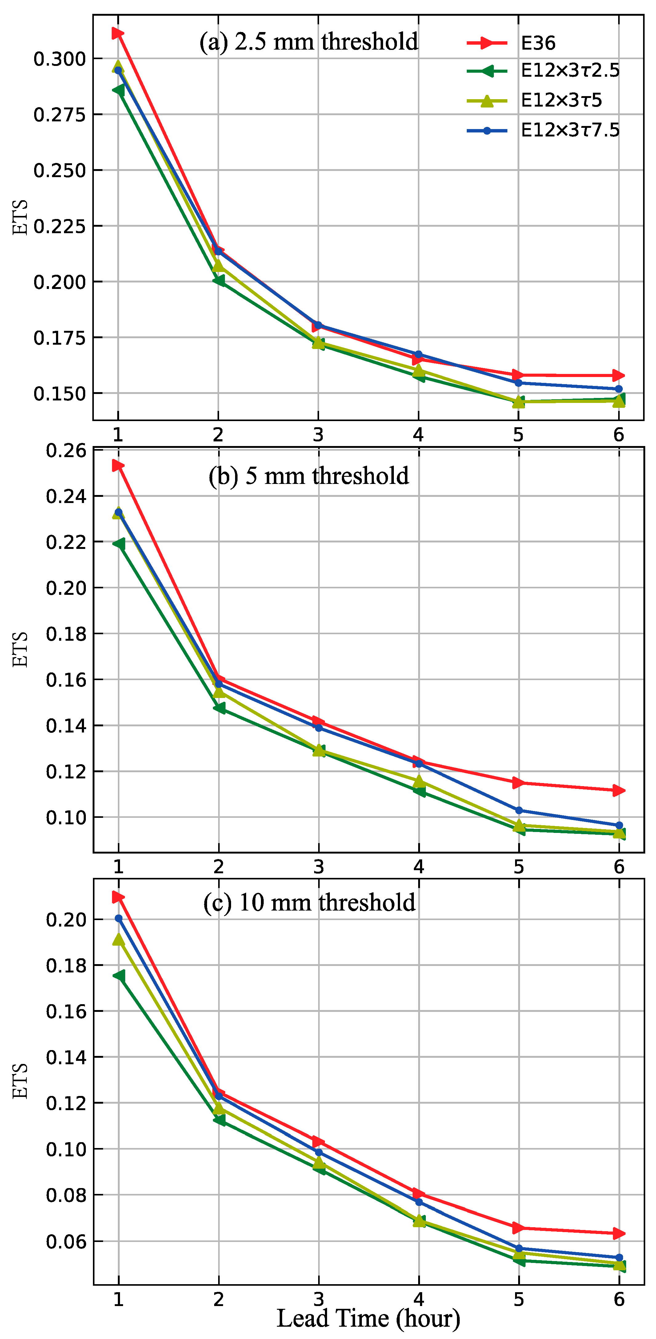
To evaluate the overall performances of the precipitation forecasts, the probability-matched (PM) ensemble means [29] of hourly accumulated precipitation forecasts were calculated for the four severe storm events in each experiment and verified against the Stage IV multi-sensor observed/estimated hourly rainfall (hereafter referred to as observed hourly rainfall) from the National Centers for Environmental Prediction [30]. Here, as explained in [29], the PM mean was used to address the issues with traditional ensemble-mean-precipitation forecasts, which often underestimate extreme precipitation events and exhibit smoothed spatial patterns. By increasing the sizes of the large precipitation areas and shrinking or eliminating the smaller areas, the PM mean preserved the spatial structure of the ensemble mean while incorporating the distribution of the amounts of precipitation from the individual ensemble members, resulting in a more accurate precipitation forecast that retained higher amplitudes and exhibited a bias that was approximately equal to the average bias of the ensemble members. At this point, by using 2.5-mm, 5-mm, or 10-mm thresholds for hourly accumulated precipitation, the equitable threat score (ETS; [31]) was calculated for the PM ensemble mean of the hourly accumulated precipitation in each forecast and then averaged over not only the 11 forecasts (initiated hourly from 1700 UTC to 0300 UTC the next day) but also the four severe storm events for each type of experiment.
The averaged ETSs calculated using 2.5-mm, 5-mm and 10-mm thresholds are shown by the differently colored curves for the four types of experiment as functions of the forecast lead time in Figure 6a–c. As shown in each panel in Figure 6, the averaged ETS calculated from the E12×3τ7.5 was very close to that from the E36, especially for the 2–4 h forecasts, although it was slightly below that from the E36 for the 5–6 h forecasts. The averaged ETSs from the E12×3τ2.5 and E12×3τ5 were also close to those from the E36, but they were slightly below those from the E12×3τ7.5 and E36.
The statistical method of single-factor variance analysis [32] was used to determine whether the average ETSs from the four types of experiment, referred to as the four groups, were statistically significant. In this case, for each forecast lead time and each threshold, we sampled 11 × 4 = 44 ETSs from eleven forecasts over the four events in each group, so the F-value, calculated as a random variable from the between-group variance divided by the sum of within-group variances, obeyed the Fm,n distribution, with (m, n) = (4 − 1, 44 − 4) = (3, 40), where m (or n) is the degree of freedom calculated for computing the between-group variance (or the sum of the within-group variances). The F-values calculated for the three forecast lead times are listed in each row in Table 4 for each threshold. Clearly, these F-values were all much lower than the critical value of Fα = 4.31 (or 2.84), taken from the Fm,n distribution for the α = 1% (or 5%) significance level. This validated the null hypothesis, namely, that there were no significant differences between the average ETSs from the four types of experiment for each forecast lead time and each threshold.
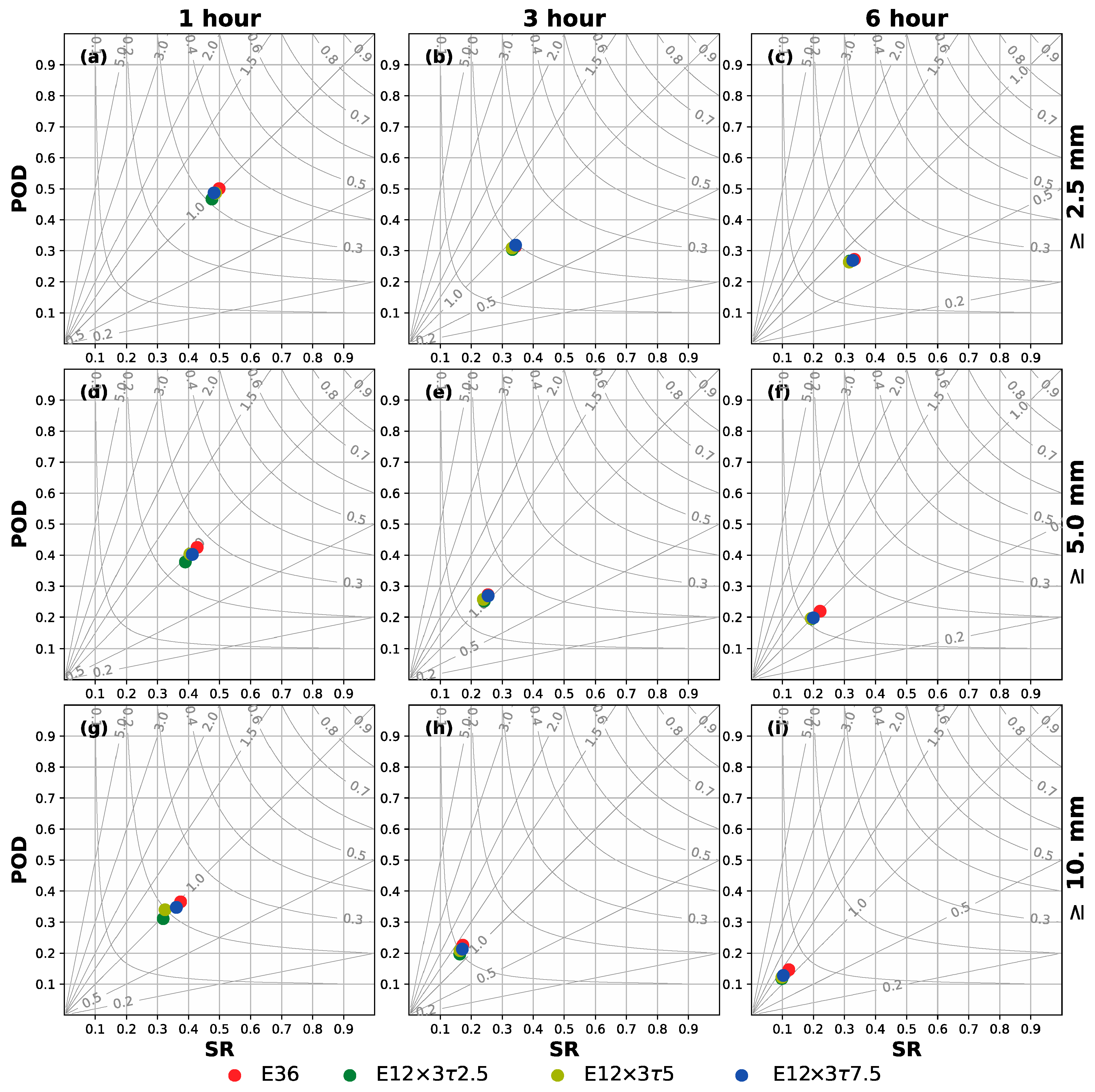
To provide a broader view of the forecast accuracies produced from each type of experiment, contingency-based metrics were calculated (by using 2.5-mm, 5-mm and 10-mm thresholds) for the PM ensemble means of the hourly accumulated precipitation forecasts in each type of experiment. These metrics included four contingency elements: the probability of detection (POD), the success ratio (SR) or false alarm rate (FAR = 1 − SR), the critical success index (CSI) and the frequency bias (FB). To provide a concise and clear depiction of the forecast performance, the four contingency elements were merged into one graph—the categorical-performance diagram [33]. Performance diagrams of this type are plotted in the 3 × 3 panels in Figure 7 to show the average accuracy scores calculated using three different thresholds for the forecasts with three different lead times from each type of experiment, while the average was taken as described above for the averaged ETSs.
Note that the forecast accuracy increased as the POD, SR, CSI and FB all approached one, meaning that the perfect forecast lies in the upper-right corner of the diagram, while the forecast accuracy decreased as the POD, SR and CSI approached zero and the FB approached infinity, meaning that the worst forecast lies on the lower-left corner of the diagram. Thus, among the four colored dots in each diagram, the dot located closest to the upper right corner shows the highest accuracy score, while the dot located closest to the lower-left corner shows the lowest accuracy score. Based on this information, it is apparent, from Figure 7, that the four types of experiment had very similar forecast accuracies, which decreased successively as the forecast lead time increased from 1 to 3 and, subsequently, to 6 h. The results in Figure 7 indicate that the three TES experiments had nearly the same accuracy levels in terms of precipitation forecasting as the E36 and, further, that the precipitation-forecast accuracy was not sensitive to τ, although the accuracy improved slightly/slowly and became increasingly close to that of the E36 as the τ increased from 2.5 min to 5 min and, subsequently, to 7.5 min.

4.2.2. Best Forecast-Performance Case: 28 April 2021 Severe Storm Event

For the severe storm event on 28 April 2021, the PM ensemble means of the hourly accumulated precipitation generated from 1-h, 3-h and 6-h forecasts valid at 0200 UTC on 29 April in each experiment are plotted in Figure 8, while the observed hourly rainfall (also valid at 0200 UTC on 29 April) is plotted in the last panel at the bottom of Figure 8. As shown in the first column in Figure 8, the PM ensemble means of the hourly accumulated precipitation forecasts from the four experiments had very similar overall distributions and intensities and the PM ensemble mean from the E12×3τ7.5 was slightly closer to that from the E36 (and also closer to the observed hourly rainfall) than those from the E12×3τ2.5 and E12×3τ5. When the forecast lead time increased to 3 and 6 h, the PM ensemble means from the four experiments remained close to each other, but their distance from the observed hourly rainfall decreased, as shown, respectively, in the second and third columns of Figure 8. Thus, regardless of the increase in the forecast lead time, the PM ensemble means for the hourly accumulated precipitation forecasts from the three TES experiments had about the same predictive capability as that from the E36 and, further, this capability was not sensitive to τ, although τ = 7.5 min appears to have been optimal.
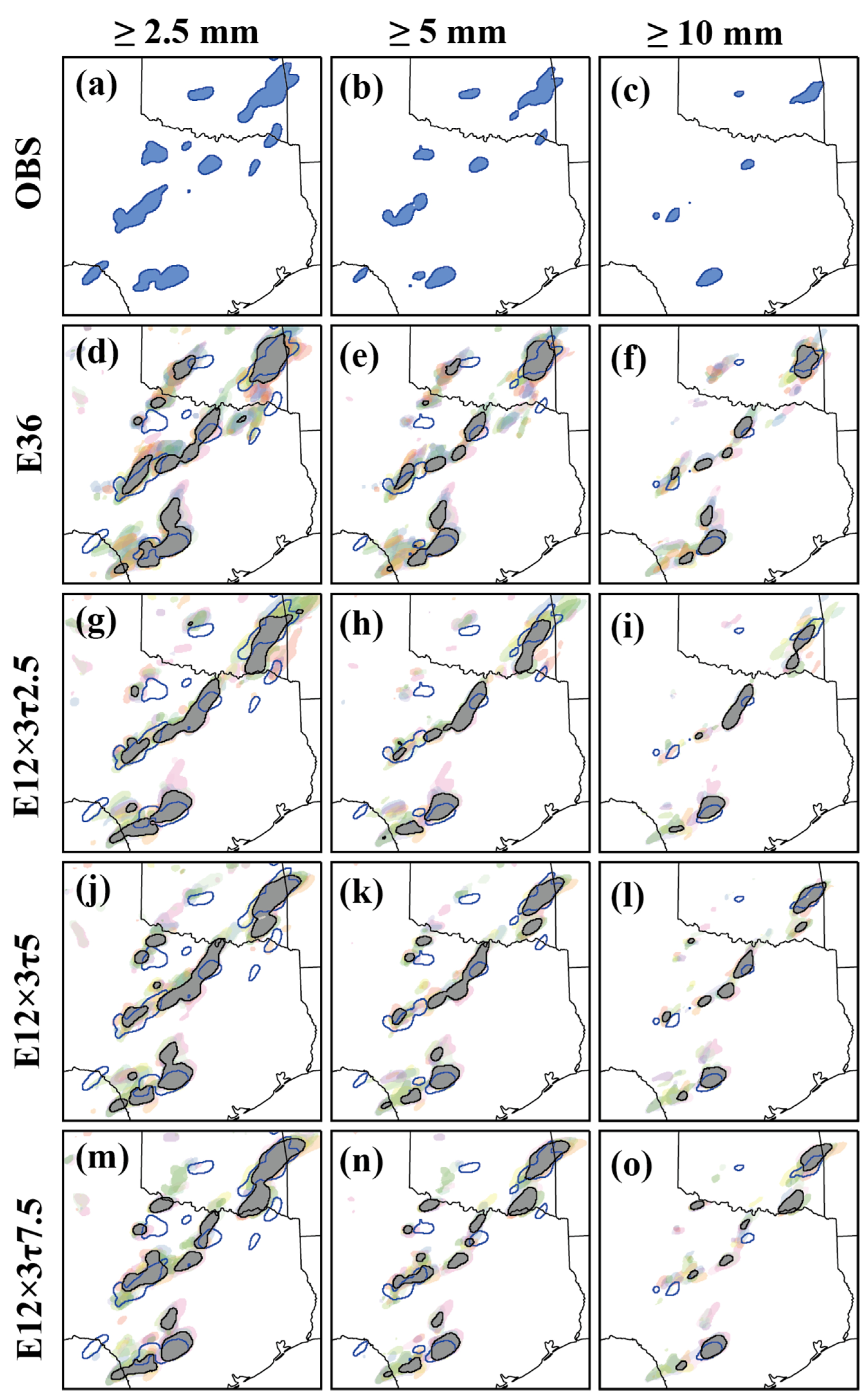
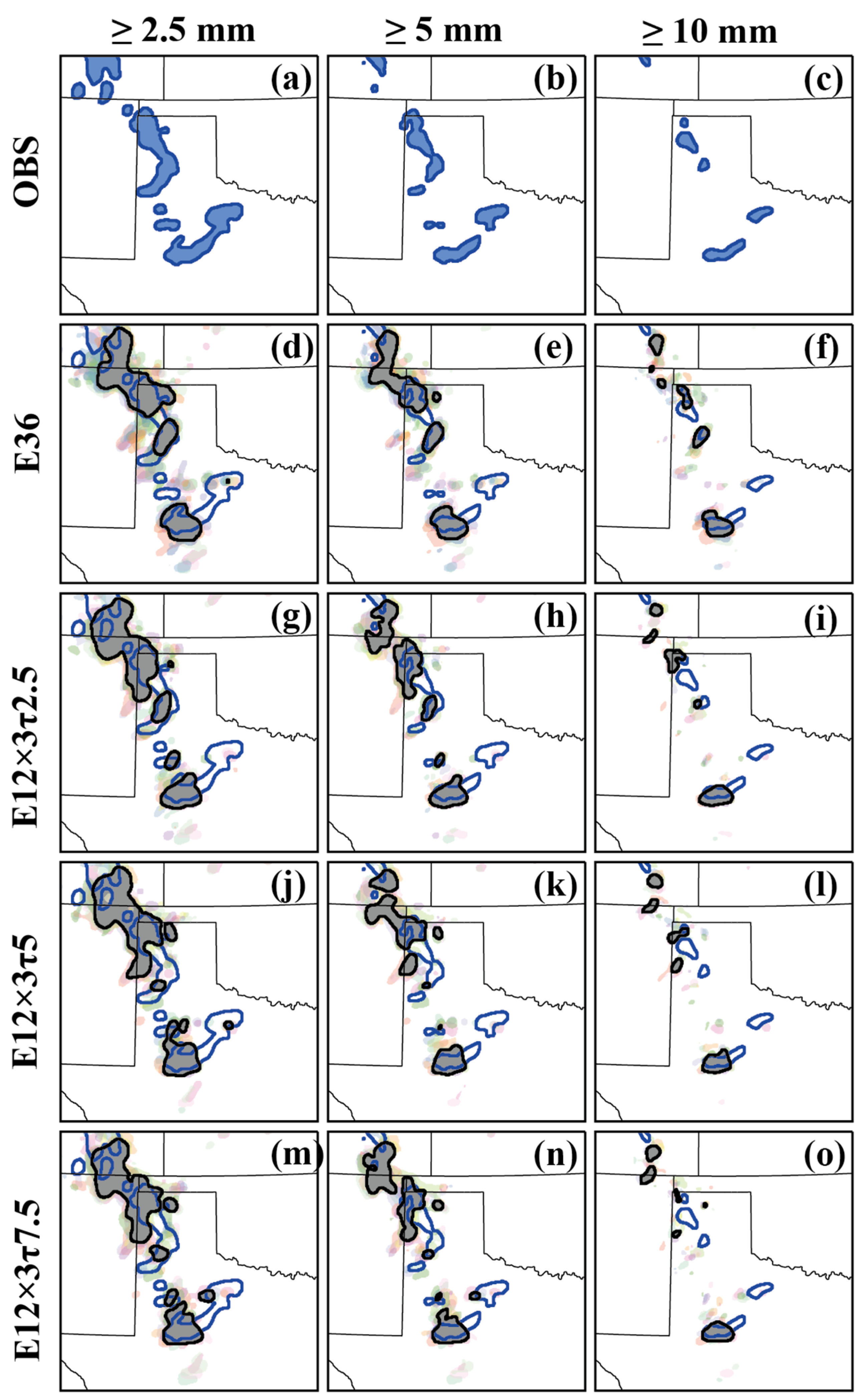
The object-based verification method [34] was also used to assess the quality of hourly accumulated precipitation forecasts versus the observed hourly rainfall. The observed objects were defined as areas of hourly rainfall ≥ 2.5 (5 or 10) mm in the observed hourly rainfall. The observed objects at 0200 UTC 29 on April 2021 are shown by the blue shades outlined by blue loops in the first, second and third panels in the top row in Figure 9. The forecasted objects in the PM ensemble mean (or an individual ensemble members) were defined as the areas of hourly accumulated precipitation ≥ 2.5 mm, 5 mm or 10 mm in the forecasted PM ensemble mean (or on individual ensemble members). The forecasted objects determined by using each of the three thresholds from the 3-h forecast in each experiment are shown in each row below the top row in Figure 9.
As shown in each column in Figure 9 for each selected hourly rainfall threshold, the observed objects were closely matched with the forecasted objects in the PM ensemble mean (although they were not well matched with the forecasted objects in the individual ensemble members) produced in each experiment. In addition, the four experiments, especially the three TES experiments, produced similar forecasted objects in the PM ensemble mean for each selected threshold. This feature was unchanged when the forecast lead time changed from 3 h to 1 h (or 6 h), although the forecasted objects matched the observed objects more (or less) closely than those shown in Figure 9. Thus, as the computational efficiency was improved by the TES, the quality of the PM ensemble mean of the hourly accumulated precipitation forecast was affected little by the TES and was not sensitive to τ.
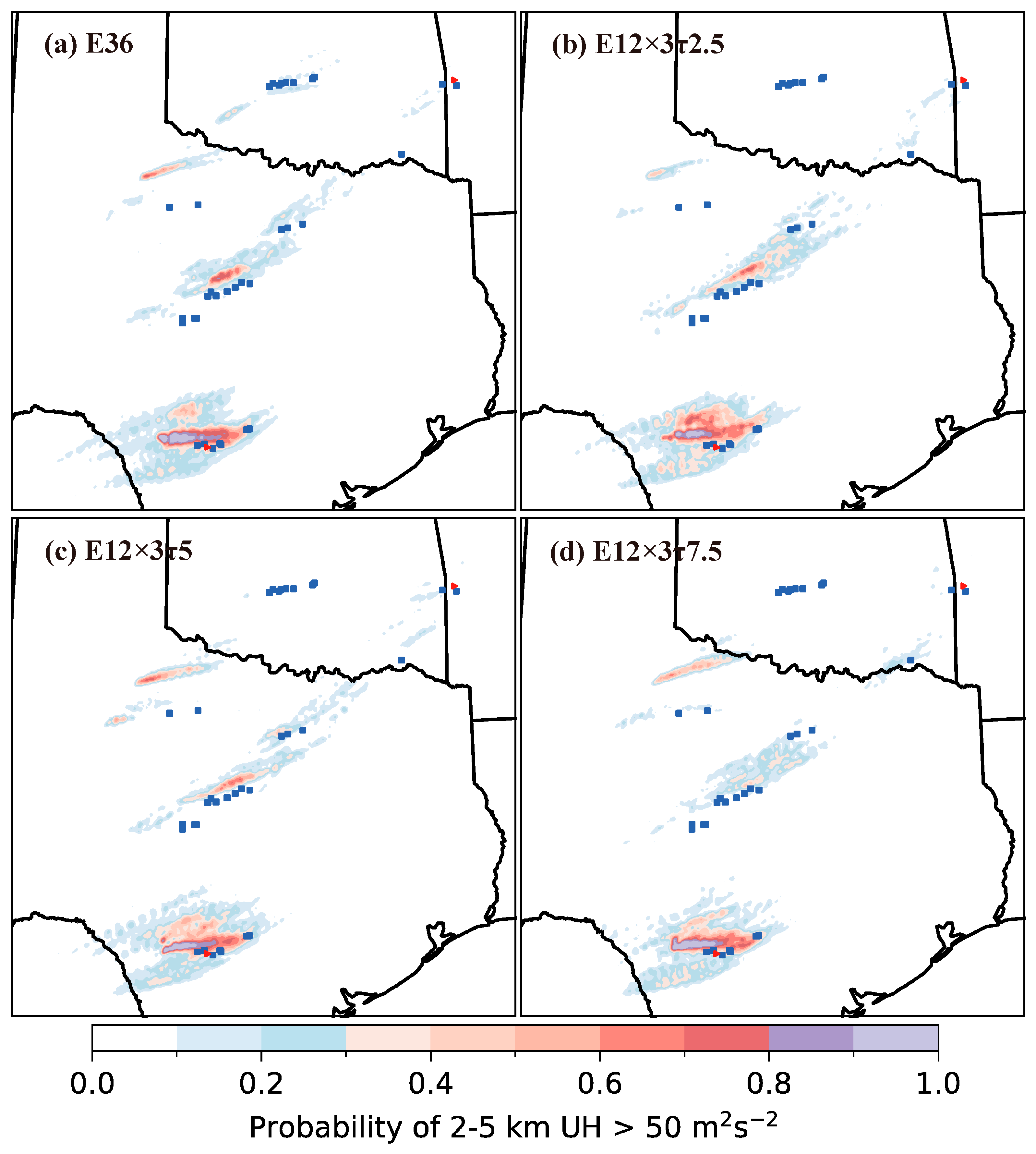
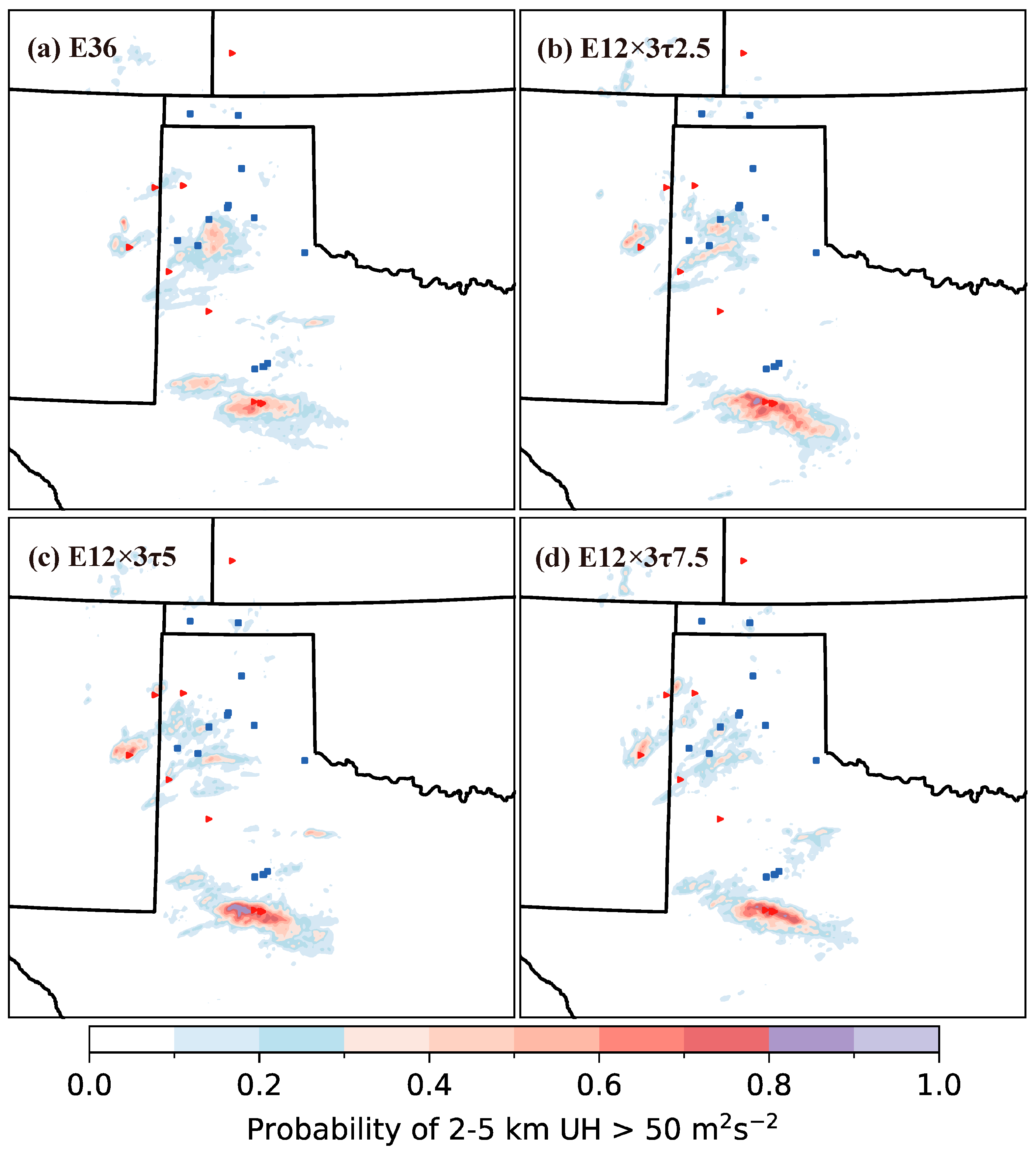
Forecasts of strong updraft helicity (UH) in the vertical layer 2–5 km above the ground (called the 2–5 km UH) can be used as gauges of mesocyclone forecasts [35] and verified against local storm reports issued by the National Weather Service. To perform this type of verification for the event on 28 April 2021, the velocity field forecasted from each ensemble member in each experiment was preprocessed in the following three steps: (i) Calculate the 2–5 km UH at each horizontal grid point from the forecasted velocity field over the 6-h-forecast time period starting from 2300 UTC. (ii) Search for the maximum 2–5 km UH over the 6-h-forecast time period at each horizontal grid point. (iii) Derive the probability of the maximal 2–5 km UH > 50 m2s−2 from the ensemble of the maximal 2–5 km UH obtained in step (ii) at each horizontal grid point for each experiment. The horizontal field of the derived probability forecast was plotted for each experiment in each panel in Figure 10 against the reported locations of the tornadoes (shown by the red triangles) and damaging winds (shown by the blue squares) occurring during the 6-h time period starting from 2300 UTC on 28 April.
As shown in each panel in Figure 10, the forecasted probability (of the maximal 2–5 km UH > 50 m2s−2) was very high (>80%) near the reported locations of the tornadoes (shown by the red triangle) and damaging winds (shown by the five blue squares) near San Antonio and, further, the forecasted probability was also high (>40%) along the reported locations of damaging winds (shown by a series of 14 blue squares) extending from Central Texas towards Oklahoma, although the forecasted probability was low (<20%) around the reported locations of the tornadoes (shown by a red triangle) and damaging winds (shown by two blue squares) near the eastern boundary of Oklahoma. These verifications indicate that the velocity forecasts from the three TES experiments had about the same capability and quality as that from the E36 for the probabilistic prediction of tornadoes and damaging winds and, further, that the capability and quality of the probabilistic prediction were not sensitive to τ (specified between 2.5 and 7.5 min).

4.2.3. Worst Forecast-Performance Case: 17 May 2021 Severe Storm Event

For the severe storm event on 17 May 2021, the PM ensemble means of the hourly accumulated precipitations from the 1-h, 3-h and 6-h forecasts valid at 0100 UTC on 18 May are plotted in three panels in each row in Figure 11 for each experiment, in comparison with the observed hourly rainfall (also valid at 0100 UTC on 18 May) plotted in the last panel at the bottom of Figure 11. As shown in Figure 11, in comparison with Figure 8, the PM ensemble means from the four experiments also had very similar overall distributions and intensities and, further, the PM ensemble mean from the E12×3τ7.5 was also slightly closer to that from the E36 (and also closer to the observed hourly rainfall, at least, for the 1-h forecast) than those from the E12×3τ2.5 and E12×3τ5 (for each forecast lead time, as shown in each column). However, when the forecast lead time increased to 3 (or 6) hours, the differences between PM ensemble means from the four experiments and the observed hourly rainfall became greater than the differences shown for the event on the 28 April 2021 in the second (or third) column in Figure 8. Despite the degraded predictive capabilities for this event, which had the worst forecast, the PM ensemble means for the hourly accumulated precipitation forecasts from the three TES experiments maintained a similar predictive capability to that from the E36 and, further, this capability was still not sensitive to τ.
The object-based verification method was used again to assess the quality of the hourly accumulated precipitation forecasts compared to the observed hourly rainfall for the event on 17 May 2021. Figure 12 plots the forecasted objects versus the observed objects valid at 0100 UTC on 18 May for the event on 18 May 2021 in a manner that is similar to those plotted in Figure 9 (valid at 0200 UTC for the event on 28 April 2021). As shown in each column in Figure 12 for each selected hourly rainfall threshold, the observed objects were still largely matched with the forecasted objects in the PM ensemble mean from each experiment, but not as closely as those shown in Figure 9 for the event on 28 April 2021. The four experiments, especially the three TES experiments, still produced similar forecasted objects in the PM ensemble mean for each selected threshold. This feature was still unchanged when the forecast lead time changed from 3 h to 1 h (or 6 h), although the forecasted objects matched the observed objects more (or less) closely than those shown in Figure 12. Thus, the quality of the PM ensemble mean of the hourly accumulated precipitation forecast was still affected little by the TES and was not sensitive to τ for the event on 17 May 2021.
Figure 13 plots the horizontal field of the probability forecasts derived from the four experiments against the reported locations of the tornadoes (shown by the three red triangles) and damaging winds (shown by the blue squares) occurring during the 6-h time period starting from 2200 UTC on 17 May. As demonstrated in each panel in Figure 13, the forecasted probability (of the maximal 2–5 km UH > 50 m2s−2) was very high (>70% for the E36 in panel (a) and >80% for the three TES experiments in panels (b)–(d)) at and around the reported location of the tornado (shown by the three densely packed red triangles) in Central Texas. The forecasted probability was also high (>40% for the E36 in panel (a) and >50% for the three TES experiments in panels (b–d)) near the reported location of the tornado (shown by the red triangle) in New Mexico, outside the western boundary of Texas, but the forecasted high probability over a broad area of North Central Texas did not closely match the reported locations of the tornadoes and damaging winds scattered in this broad area. These verifications reaffirm that the velocity forecasts from the three TES experiments had about the same capability and quality as that from the E36 for the probabilistic prediction of tornadoes and damaging winds and, further, that the capability and quality of the probabilistic prediction were not sensitive to τ, although they were all degraded for this event, which had the worst forecast.

5. Conclusions

In this paper, the cost-saving time-expanded sampling (TES) approach [10,11] was applied to the convection-allowing ensemble-based warn-on-forecast system (WoFS) in EnKF assimilations of remote-sensing data from radars and the geostationary satellite GOES-16 to generate short-term (0–6-h) forecasts for four severe storm events that occurred in the southern and/or central US in April and May 2021. For each event, TES was compared with a 36-member control experiment (E36) by reducing the forecast ensemble size to 12 while tripling the analysis ensemble size to 12 × 3 = 36 with the TES time interval set to τ = 2.5 min, 5 min and 7.5 min in the three TES experiments. The assimilation statistics were evaluated for each TES experiment versus the E36 for each event and, further, the forecasts produced in each experiment (including the E36) were verified against multi-sensor observed/estimated rainfall, reported tornadoes and damaging winds for each event. The main results are summarized below:
(i)
Under various severe-weather conditions, represented by the four severe storm events considered in this study, TES can be successfully applied to the WoFS in assimilating remote-sensing data from radars and the geostationary satellite GOES-16, with improved computational efficiency and without compromising the quality of the analysis and subsequent short-term prediction of high-impact weather.
(ii)
With a wide range of severe-weather scenarios to capture, there is an optimal sampling-time interval τ, which can lead to better analyses and subsequent predictions. For the wide range of severe-weather scenarios (overviewed in Section 3.1 for the four severe storm events) in this study, the optimal sampling-time interval was found to be τ = T/2 (where T = 15 min is the assimilation-cycle-time window), although the quality of the analysis and the subsequent predictive capability were not sensitive to τ (selected between T/6 and T/2).
The results summarized above suggest that TES is appealing and useful for cost-saving real-time applications of WoFS in the assimilation of remote-sensing data and the generation of short-term severe-weather forecasts. For data-assimilation cycles, the model integration for each updating run in the E36 uses two cores with the NSSL supercomputer. In total, 36 × 2 = 72 cores were used for the ensemble model integration during one data-assimilation window. The use of TES reduced the number of updating runs to one third of that in the E36 and, thus, reduced the number of cores from 72 used in E36 to only 12 × 2 = 24. Note that the integration time for each updating run in the TES experiment with τ = T/6 (or T/2) increased from T in the E36 to 7T/6 (or 3T/2), so the computational cost for the data-assimilation cycles in the TES experiment is 7/18 (or 1/2) of the cost for those in the E36, demonstrating a saving of 11/18 (or 1/2) of the computational cost. However, in terms of the computer storage for the data assimilation, both the E36 and the TES runs used about the same space. Although only 12 members of the model run needed to be saved, the model fields at two extra time levels consumed a portion of the disk space. For each forecast at the top of each hour, the E36 experiment ran with 18 ensemble members (36 cores) and each TES experiment ran with 12 members (24 cores), implying an unfair advantage for the E36 in terms of forecast-quality evaluations (because the forecast ensemble size in each TES experiment was smaller than that in the E36), but the computational cost for the forecast runs in each TES experiment was lower than those in the E36.
According to the results obtained with simulated radar observations in [11], further increases in τ beyond T/2 do not significantly improve the analysis and forecast, but they do increase the computational cost significantly, as explained above. Thus, for real-time applications of TES with the WoFS, an optimal τ should be selected by properly balancing the two competing factors: (i) increasing τ (beyond T/2) to further improve the analysis and forecast; and (ii) decreasing τ (below T/2) to further reduce the computational cost. The results obtained in this study suggest that an optimal selection can be achieved by setting τ = T/2, although the question of how to properly balance the two competing factors requires continued research beyond this study.
The insensitivity to τ is particularly attractive for real-time applications, as it implies that labor-intensive adaptive tuning and/or the cumbersome event-based selection of τ can be avoided or skipped in preparing TES for the future real-time applications described in this study. However, in general, the proper selection of τ should be confined within a scale-dependent range that is consistent with the spatial and temporal scales of the main weather system covered and resolved by the model and observing system. This scale dependence was shown in previous real-data applications of TES [13,14,15,16]. Consequently, the question of how to properly select multiple scale-dependent values of τ to apply TES to the new weather-adaptive dual-resolution hybrid WoFS remains open [36]. Addressing this issue is crucial to produce cost-saving real-time implementations of this new hybrid WoFS and requires continued research on TES beyond this study.

Author Contributions

Experiment validation, formal analysis, visualization and writing—original draft and review/revision: H.Z. Data curation, validation and writing—original draft and review/revision: J.G. Methodology, writing—original draft and review/revision, supervision and funding acquisition: Q.X. Manuscript review/revision, project administration and funding acquisition: L.R. All authors have read and agreed to the published version of the manuscript.

Funding

The research work was supported by an award from the NSSL Warn-on-Forecast project and the Office of Naval Research, number N000142012449, to the University of Oklahoma (OU) and by the National Natural Science Foundation of China, grant 42275010, awarded to the Institute of Atmospheric Physics.

Data Availability Statement

The community version 1.3 of [GSI-EnKF] data assimilation software can be downloaded from https://dtcenter.org/community-code/gridpoint-statistical-interpolation-gsi/download (accessed on 25 April 2023). The [WRF] source code version 3.9.1 is publicly available at NCAR/UCAR (https://github.com/wrf-model/WRF (accessed on 25 April 2023)). The [WSR-88D Level-II] data (reflectivity factor and radial velocity) used in this research can be accessed at http://www.ncdc.noaa.gov/ by filling in locations of radar site and date. All other dataset and code used to generate these results are available from the authors upon request.

Acknowledgments

The authors are thankful to Yunheng Wang at NSSL and the two anonymous reviewers for providing constructive comments and suggestions.

Conflicts of Interest

The authors declare no conflict of interest.

References

  1. NOAA. Strategic plan for NOAA’s Office of Oceanic and Atmospheric Research. NOAA Rep. 2. 2014. Available online: https://research.noaa.gov/sites/oar/Documents/OARStrategicPlan.pdf (accessed on 25 April 2023).
  2. Stensrud, D.J.; Xue, M.; Wicker, L.J.; Kelleher, K.E.; Foster, M.P.; Schaefer, J.T.; Schneider, R.S.; Benjamin, S.; Weygandt, S.S.; Ferree, J.T.; et al. Convective-scale warn-on-forecast system: A vision for 2020. Bull. Am. Meteorol. Soc. 2009, 90, 1487–1500. [Google Scholar] [CrossRef]
  3. Stensrud, D.J.; Wicker, L.J.; Xue, M.; Dawson, D.T.; Yussouf, N.; Wheatley, D.M.; Thompson, T.E.; Snook, N.A.; Smith, T.M.; Schenkman, A.D.; et al. Progress and challenges with Warn-on-Forecast. Atmos. Res. 2013, 123, 2–16. [Google Scholar] [CrossRef]
  4. Wheatley, D.M.; Knopfmeier, K.H.; Jones, T.A.; Creager, G.J. Storm-scale data assimilation and ensemble forecasting with the NSSL experimental warn-on-forecast system. Part I: Radar data experiments. Weather Forecast. 2015, 30, 1795–1817. [Google Scholar] [CrossRef]
  5. Jones, T.A.; Wang, X.; Skinner, P.; Johnson, A.; Wang, Y. Assimilation of GOES-13 imager clear-sky water vapor (6.5 μm) Radiances into a Warn-on-Forecast System. Mon. Weather Rev. 2018, 146, 1077–1107. [Google Scholar] [CrossRef]
  6. Flora, M.L.; Skinner, P.; Potvin, C.K.; Reinhart, A.E.; Jones, T.A.; Yussouf, N.; Knopfmeier, K.H. Object-based verification of short-term, storm-scale probabilistic mesocyclone guidance from an experimental Warn-on-Forecast System. Weather Forecast. 2019, 34, 1721–1739. [Google Scholar] [CrossRef]
  7. Yussouf, N.; Knopfmeier, K.H. Application of the Warn-on-Forecast system for flash-flood-producing heavy convective rainfall events. Q. J. R. Meteorol. Soc. 2019, 145, 2385–2403. [Google Scholar] [CrossRef]
  8. Jones, T.A.; Skinner, P.; Yussouf, N.; Knopfmeier, K.; Reinhart, A.; Wang, X.; Bedka, K.; Smith, W.; Palikonda, R. Assimilation of GOES-16 radiances and retrievals into the Warn-on-Forecast System. Mon. Weather Rev. 2020, 148, 1829–1859. [Google Scholar] [CrossRef]
  9. Guerra, J.E.; Skinner, P.S.; Clark, A.; Flora, M.; Matilla, B.; Knopfmeier, K.; Reinhart, A.E. Quantification of NSSL Warn-on-Forecast System accuracy by storm age using object-based verification. Weather Forecast. 2022, 37, 1973–1983. [Google Scholar] [CrossRef]
  10. Xu, Q.; Wei, L.; Lu, H.; Qiu, C.; Zhao, Q. Time-expanded sampling for ensemble-based filters: Assimilation experiments with a shallow-water equation model. J. Geophys. Res. Atmos. 2008, 113. [Google Scholar] [CrossRef]
  11. Xu, Q.; Lu, H.; Gao, S.; Xue, M.; Tong, M. Time-expanded sampling for ensemble Kalman filter: Assimilation experiments with simulated radar observations. Mon. Weather. Rev. 2008, 136, 2651–2667. [Google Scholar] [CrossRef]
  12. Gustafsson, N.; Bojarova, J.; Vignes, O. A hybrid variational ensemble data assimilation for the High Resolution Limited Area Model (HIRLAM). Nonlinear Process Geophys. 2014, 21, 303–323. [Google Scholar] [CrossRef]
  13. Huang, B.; Wang, X. On the use of cost-effective Valid-Time-Shifting (VTS) method to increase ensemble size in the GFS Hybrid 4DEnVar System. Mon. Weather. Rev. 2018, 146, 2973–2998. [Google Scholar] [CrossRef]
  14. Gasperoni, N.A.; Wang, X.; Wang, Y. Using a cost-effective approach to increase background ensemble member size within the GSI-Based EnVar System for improved radar analyses and forecasts of convective systems. Mon. Weather. Rev. 2022, 150, 667–689. [Google Scholar] [CrossRef]
  15. Lu, H.; Xu, Q.; Yao, M.; Gao, S. Time-expanded sampling for ensemble-based filters: Assimilation experiments with real radar observations. Adv. Atmos. Sci. 2011, 28, 743–757. [Google Scholar] [CrossRef]
  16. Zhao, Q.; Xu, Q.; Jin, Y.; McLay, J.; Reynolds, C. Time-expanded sampling for ensemble-based data assimilation applied to conventional and satellite observations. Weather Forecast. 2015, 30, 855–872. [Google Scholar] [CrossRef]
  17. Skamarock, W.C.; Klemp, J.B.; Dudhia, J.; Gill, D.O.; Barker, D.M.; Duda, M.G.; Huang, X.-Y.; Wang, W.; Powers, J.G. A Description of the Advanced Research WRF Version 3; National Center For Atmospheric Research Boulder Co Mesoscale and Microscale Meteorology Div: Boulder, CO, USA, 2008. [Google Scholar]
  18. Liu, H.; Hu, M.; Ge, G.; Zhou, C.; Stark, D.; Shao, H.; Newman, K.; Whitaker, J. Ensemble Kalman Filter (EnKF) User’s Guide Version 1.3-Compatible with GSI Community Release v3.7. 2018. Available online: https://dtcenter.org/community-code/ensemble-kalman-filter-system-enkf/documentation (accessed on 25 April 2023).
  19. Jones, T.A.; Otkin, J.A.; Stensrud, D.J.; Knopfmeier, K. Assimilation of satellite infrared radiances and doppler radar observations during a cool season observing system simulation experiment. Mon. Weather Rev. 2013, 141, 3273–3299. [Google Scholar] [CrossRef]
  20. McPherson, R.A.; Fiebrich, C.A.; Crawford, K.C.; Kilby, J.R.; Grimsley, D.L.; Martinez, J.E.; Basara, J.; Illston, B.G.; Morris, D.A.; Kloesel, K.A.; et al. Statewide monitoring of the mesoscale environment: A technical update on the Oklahoma Mesonet. J. Atmos. Ocean. Technol. 2007, 24, 301–321. [Google Scholar] [CrossRef]
  21. Weng, F. Advances in radiative transfer modeling in support of satellite data assimilation. J. Atmos. Sci. 2007, 64, 3799–3807. [Google Scholar] [CrossRef]
  22. Whitaker, J.S.; Hamill, T.M.; Wei, X.; Song, Y.; Toth, Z. Ensemble data assimilation with the NCEP Global forecast system. Mon. Weather Rev. 2008, 136, 463–482. [Google Scholar] [CrossRef]
  23. Gaspari, G.; Cohn, S.E. Construction of correlation functions in two and three dimensions. Q. J. R. Meteorol. Soc. 1999, 125, 723–757. [Google Scholar] [CrossRef]
  24. Zhang, J.; Howard, K.W.; Langston, C.; Kaney, B.; Qi, Y.; Tang, L.; Grams, H.; Wang, Y.; Cocks, S.; Martinaitis, S.M.; et al. Multi-Radar Multi-Sensor (MRMS) quantitative precipitation estimation: Initial operating capabilities. Bull. Am. Meteorol. Soc. 2016, 97, 621–638. [Google Scholar] [CrossRef]
  25. Smith, T.M.; Lakshmanan, V.; Stumpf, G.J.; Ortega, K.; Hondl, K.; Cooper, K.; Calhoun, K.; Kingfield, D.; Manross, K.L.; Toomey, R.; et al. Multi-Radar Multi-Sensor (MRMS) severe weather and aviation products: Initial operating capabilities. Bull. Am. Meteorol. Soc. 2016, 97, 1617–1630. [Google Scholar] [CrossRef]
  26. Benjamin, S.G.; Weygandt, S.S.; Brown, J.M.; Hu, M.; Alexander, C.R.; Smirnova, T.G.; Olson, J.B.; James, E.; Dowell, D.C.; Grell, G.A.; et al. A north american hourly assimilation and model forecast cycle: The rapid refresh. Mon. Weather Rev. 2016, 144, 1669–1694. [Google Scholar] [CrossRef]
  27. Mansell, E.R.; Ziegler, C.L.; Bruning, E. Simulated electrification of a small thunderstorm with two-moment bulk microphysics. J. Atmos. Sci. 2010, 67, 171–194. [Google Scholar] [CrossRef]
  28. Pan, S.; Gao, J. A method for assimilating pseudo dewpoint temperature as a function of GLM flash extent density in GSI-based EnKF data assimilation system—A proof of concept study. Earth Space Sci. 2022, 9, 2378. [Google Scholar] [CrossRef]
  29. Clark, A.J. Generation of ensemble mean precipitation forecasts from convection-allowing ensembles. Weather Forecast. 2017, 32, 1569–1583. [Google Scholar] [CrossRef]
  30. Baldwin, M.E.; Mitchell, K.E. The NCEP hourly multisensor US precipitation analysis for operations and GCIP research. In Proceedings of the Preprints, 13th Conference on Hydrology, Long Beach, CA, USA, 13–17 January 1997; Volume 54, p. 55. [Google Scholar]
  31. Wilks, D.S. Statistical Methods in the Atmospheric Sciences. (International Geophysics), 3rd ed.; Academic Press: Cambridge, MA, USA, 2011; Volume 100. [Google Scholar]
  32. Snedecor, G.W.; Cochran, W.G. Statistical Methods, 8th ed.; Iowa State University Press: Ames, IA, USA, 1989. [Google Scholar]
  33. Roebber, P.J. Visualizing multiple measures of forecast quality. Weather Forecast. 2009, 24, 601–608. [Google Scholar] [CrossRef]
  34. Davis, C.; Brown, B.; Bullock, R. Object-based verification of precipitation forecasts. Part I: Methodology and application to mesoscale rain areas. Mon. Weather Rev. 2006, 134, 1772–1784. [Google Scholar] [CrossRef]
  35. Kain, J.S.; Weiss, S.J.; Bright, D.R.; Baldwin, M.E.; Levit, J.J.; Carbin, G.W.; Schwartz, C.S.; Weisman, M.L.; Droegemeier, K.K.; Weber, D.B.; et al. Some practical considerations regarding horizontal resolution in the first generation of operational convection-allowing NWP. Weather Forecast. 2008, 23, 931–952. [Google Scholar] [CrossRef]
  36. Wang, Y.; Gao, J.; Skinner, P.S.; Knopfmeier, K.; Jones, T.; Creager, G.; Heiselman, P.L.; Wicker, L.J. Test of a Weather-adaptive dual-resolution hybrid warn-on-forecast analysis and forecast system for several severe weather events. Weather Forecast. 2019, 34, 1807–1827. [Google Scholar] [CrossRef]
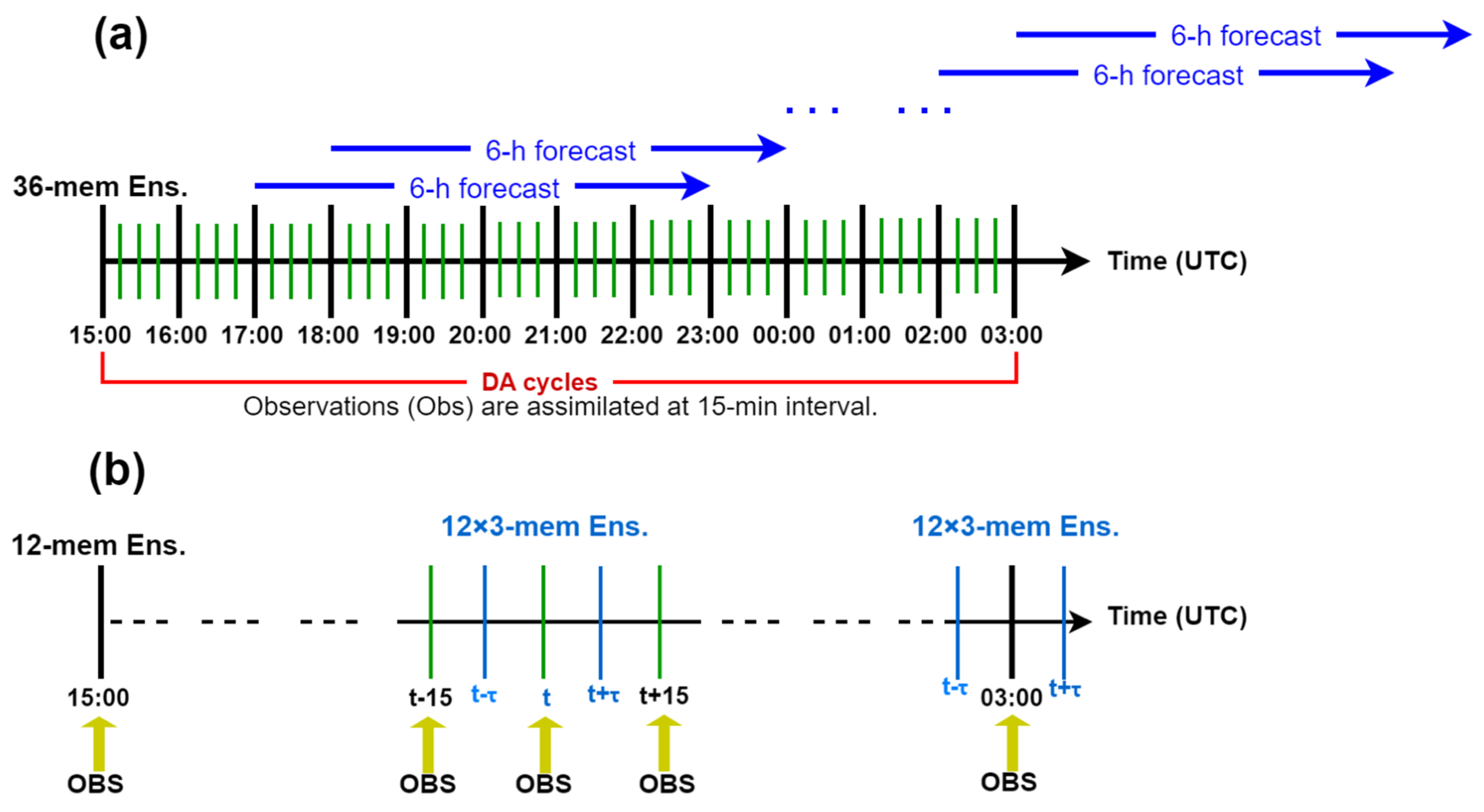
Figure 1. (a) Timeline of EnKF data assimilation (DA) cycles used with the WoFS without time-expanded sampling (TES). (b) As in (a), but with TES.
Remotesensing 15 02358 g001
Figure 2. (a) Model domain, terrain height plotted by color shades and locations of tornadoes, hails and damaging winds (which occurred during the time period from 1800 UTC to 0900 UTC the next day, according to local storm reports issued from the National Weather Service) plotted by red triangles, green dots and blue squares, respectively, for the severe storm event on 28 April 2021. (b) As in (a) but for the event on 17 May 2021. (c) As in (a) but for the event on 23 May 2021. (d) As in (a) but for the event on 26 May 2021. The color scale for terrain height is shown on the right side of the figure. State, county and city names mentioned in the paper are annotated specifically in each panel.
Remotesensing 15 02358 g002
Figure 3. (a) Number of BT62c observations plotted by the red curve as a function of time over the entire assimilation window (49 assimilation cycles from 1500 UTC to 0300 UTC next day) for the event on 28 April 2021. (b) As in (a), but for number of reflectivity observations.
Remotesensing 15 02358 g003
Figure 4. (a) BIAS d calculated for BT62c from E36 (or E12×3τ7.5) for the event on 28 April 2021 and plotted by red (or blue) curve as a function of time (from 1500 UTC to 0300 UTC next day). (b) As in (a), but for RMSI D calculated for BT62c. (c) As in (a), but calculated for reflectivity. (d) As in (b), but calculated for reflectivity.
Remotesensing 15 02358 g004
Figure 5. (a) As in Figure 4a, but for spread s calculated for BT62c. (b) As in (a), but calculated for reflectivity. (c) As in (a), but for CR. (d) As in (c), but calculated for reflectivity.
Remotesensing 15 02358 g005
Figure 6. (a) Averaged ETSs calculated using 2.5-mm threshold for PM ensemble means of hourly accumulated precipitation forecasts plotted by differently colored curves for the four types of experiment as functions of forecast lead time. (b) As in (a), but calculated using a 5-mm threshold. (c) As in (a), but calculated using a 10-mm threshold. The average was taken over not only the 11 forecasts (initiated hourly from 1700 UTC to 0300 UTC next day) but also the four severe storm events for each type of experiment.
Remotesensing 15 02358 g006
Figure 7. (ac) Performance diagrams for averaged PM ensemble means of hourly accumulated precipitation forecasts with 1-h, 3-h and 6-h lead times, respectively, while accuracy scores calculated using 2.5-mm threshold are shown by differently colored dots for different types of experiment. (df) As in (ac), but calculated using 5-mm threshold. (gi) As in (ac), but calculated using 10-mm threshold. The CSI (or FB) values are shown by hyperbolic (or straight slanted) contour lines in each panel. Four differently colored dots, corresponding to the four different types of experiment, are shown at the bottom of the figure. The average was taken as described in the caption in Figure 6.
Remotesensing 15 02358 g007
Figure 8. (a) PM ensemble mean of hourly accumulated precipitation generated from 1-h forecast valid at 0200 UTC on 29 April in E36 for the event on 28 April 2021. (b) As in (a), but from a 3-h forecast. (c) As in (a), but from a 6-h forecast. (df) As in (ac), but generated in E12×3τ2.5. (gi) As in (ac), but generated in E12×3τ5. (jl) As in (ac), but generated in E12×3τ7.5. (m) Stage IV multi-sensor observed/estimated hourly rainfall valid at 0200 UTC on 29 April 2021.
Remotesensing 15 02358 g008
Figure 9. (ac) Observed objects of hourly rainfall ≥ 2.5 mm, 5 mm and 10 mm, respectively, valid at 0200 UTC on 29 April 2021, shown by blue shades outlined by blue loops. (df) Forecasted objects of hourly accumulated precipitation ≥ 2.5 mm, 5 mm and 10 mm, respectively, in PM ensemble mean (or different ensemble members) generated from 3-h forecast in E36 valid at 0200 UTC on 29 April 2021, shown by gray shades outlined by black loops (or different-translucent-color shades), while the contours of observed objects, shown by blue loops in panels (ac), are duplicated in (df), respectively. (gi) As in (df), but generated in E12×3τ2.5. (jl) As in (df), but generated in E12×3τ5. (mo) As in (df), but generated in E12×3τ7.5.
Remotesensing 15 02358 g009
Figure 10. (a) Probability of forecasted maximal 2–5-km UH > 50 m2s−2 (over the 6-h-forecast time period initiated at 2300 UTC) generated in E36, plotted by color shades for the event on 28 April 2021. (b) As in (a), but generated in E12×3τ2.5. (c) As in (a), but generated in E12×3τ5. (d) As in (a), but generated in E12×3τ7.5. The red triangles and blue squares in each panel partially duplicate those in Figure 1a reported for tornadoes and damaging winds, respectively, occurring during the 6-h-forecast time period (that is, from 2300 UTC to 0500 UTC the next day, rather than from 1800 UTC to 0900 UTC the next day, as shown in Figure 1a).
Remotesensing 15 02358 g010
Figure 11. As in Figure 8, but valid at 0100 UTC on 18 May for the severe storm event on 17 May 2021.
Remotesensing 15 02358 g011
Figure 12. As in Figure 9, but valid at 0100 UTC on 18 May for the severe storm event on 17 May 2021.
Remotesensing 15 02358 g012
Figure 13. As in Figure 10, but generated from the forecast initiated at 2200 UTC on 17 May for the severe storm event on 17 May 2021. The red triangles and blue squares in each panel partially duplicate those in Figure 1b, reported for tornadoes and damaging winds, respectively, which occurred during the 6-h-forecast time period (that is, from 2200 UTC to 0400 UTC the next day, rather than from 1800 UTC to 0900 UTC the next day, as shown in Figure 1b).
Remotesensing 15 02358 g013
Table 1. List of observation-error standard deviations and localization radii and depths, where p (or po) denotes the vertical level of pressure at correlated grid (or observation) point.
ObservationError Standard DeviationLocalization Radius (km)Localization Depth ln(po/p)
Temperature1.0 (°K)600.85
Dewpoint1.0 (°K)600.85
U wind1.0 (m/s)60–1000.85
V wind1.0 (m/s)60–1000.85
Pressure0.75 (hPa)600.85
Reflectivity5.0–7.0 (dBZ)180.8
Radial velocity3.0 (m/s)180.8
CWP0.025–0.2 (kg/m2)360.9
BT62c1.25 (°K)364.0
BT73c1.75 (°K)364.0
Table 2. Experiment configurations.
Experiment NameDescription
E36Ns = 36 and M = 0 without TES
E12×3τ2.5Ns = 12 and M = 1 with TES and τ = 2.5 min
E12×3τ5Ns = 12 and M = 1 with TES and τ = 5 min
E12×3τ7.5Ns = 12 and M = 1 with TES and τ = 7.5 min
Table 3. BIAS, RMSI, ensemble spread and CR for BT62c, BT73c and reflectivity averaged over all the 49 assimilation cycles from each experiment for the event on 28 April 2021.
d (BIAS in °K)D (RMSI in °K)S (Spread in °K)CR
PriorPosteriorPriorPosteriorPriorPosterior
BT62c
E360.26−0.0011.1730.5551.050.4971.533
E12×3τ2.50.260.0081.2110.6261.0380.4841.448
E12×3τ50.254−0.0011.1840.6021.060.4921.482
E12×3τ7.50.256−0.0181.1750.5661.1460.5011.532
BT73c
E360.6430.2461.5270.8161.2330.5861.727
E12×3τ2.50.6280.2491.5690.8931.2250.5641.671
E12×3τ50.6140.2511.4970.8611.2320.5741.725
E12×3τ7.50.6760.2421.5740.8201.3850.5951.736
Reflectivity
E364.7383.64211.2058.6564.5891.6580.737
E12×3τ2.54.833.81511.4849.0194.8141.6080.724
E12×3τ54.4293.30210.978.265.3731.6990.788
E12×3τ7.54.3382.97810.5297.6975.8991.7410.851
Table 4. F-values calculated for three forecast lead times and three precipitation thresholds.
Forecast Lead Time1 h3 h6 h
Threshold 2.5 mm0.3420.0940.109
5 mm0.8420.3140.621
10 mm0.8680.3070.749
Disclaimer/Publisher’s Note: The statements, opinions and data contained in all publications are solely those of the individual author(s) and contributor(s) and not of MDPI and/or the editor(s). MDPI and/or the editor(s) disclaim responsibility for any injury to people or property resulting from any ideas, methods, instructions or products referred to in the content.