Communication

The Relationship between Chlorophyll Concentration and ENSO Events and Possible Mechanisms off the Changjiang River Estuary

1
Marine Science and Technology College, Zhejiang Ocean University, Zhoushan 316000, China
2
Key Laboratory of Research on Marine Hazards Forecasting, National Marine Environmental Forecasting Center, Beijing 100081, China
3
School of Marine Sciences, Nanjing University of Information Science and Technology, Nanjing 210044, China
*
Author to whom correspondence should be addressed.
Remote Sens. 2023, 15(9), 2384; https://doi.org/10.3390/rs15092384
Submission received: 4 March 2023 / Revised: 22 April 2023 / Accepted: 25 April 2023 / Published: 2 May 2023
(This article belongs to the Section Atmospheric Remote Sensing)

Abstract

:
More and more attention has been paid to the study of the impact of extreme climatic events on the ecological environment off the Changjiang River Estuary. In this study, the relationship between the chlorophyll concentration and ENSO (El Niño Southern Oscillation) events was studied. Several potential physical mechanisms between the ENSO and chlorophyll concentration were analyzed using observation and sensitivity experiments from a high-resolution ROMS-CoSiNE coupled model (Regional Ocean Modeling System-Carbon, Oxygen, Silicon, Nitrogen and Ecosystem) off the Changjiang River Estuary. Our results indicated that the April to August averaged chlorophyll concentration off the Changjiang River Estuary was significantly correlated with the December to February averaged ENSO indices in the previous winter. The 10 m wind speed and SST (Sea Surface Temperature) affected by an ENSO event had little effect on the chlorophyll concentration, while the discharge had a significant effect on the chlorophyll concentration off the Changjiang River Estuary, and the discharge was significantly and positively correlated with the ENSO indices. We tested the effect of interannual variations of the discharge and nutrients carried by discharge on the interannual variation in the chlorophyll concentration in the ENSO events. Two sensitivity experiments showed that when the nutrients in the freshwater discharge were kept as a constant seasonal cycle, the composite differences in the chlorophyll concentration between the positive and negative ENSO phases off the Changjiang River Estuary were reduced. When there were no nutrients in the freshwater discharge, the composite differences in the chlorophyll concentration between the positive and negative ENSO phases off the Changjiang River Estuary were reduced by one order of magnitude. The discharge can modify the stratification off the Changjiang River Estuary, and the nutrients carried by the discharge play a dominant role in determining the interannual variation of the chlorophyll concentration associated with the ENSO cycles.

1. Introduction

The Changjiang River in China provides 90–95% of all riverine freshwater discharge input to the East China Sea [1,2], forming a significant freshwater plume. The freshwater plume transports nutrients into the estuary and nearby sea [3,4,5,6]. Nutrients heavily influence marine ecosystems and especially biological processes [7,8,9]. Due to the abundant nutrients carried by large freshwater discharge [10,11,12], the Changjiang River Estuary has become the most productive area of the East China Sea. Zhou et al. [13] suggested that red tides are most frequent in May, accounting for 60% of red tide events in the entire year, and that such red tides are related to the nutrients which are carried by the Changjiang River discharge. After July, the red tides gradually become less frequent with almost no red tides occurring after September in the coastal waters of the Changjiang River Estuary and Zhejiang province [14]. Zhou et al. [15] suggested that the nutrients carried by the discharge in the summer may drive the increasing chlorophyll concentration at the front of the freshwater plume of the Changjiang River Estuary. Overall, most phytoplankton blooms appear from spring to summer with the discharge levels gradually increasing around the Changjiang River Estuary.
Over the past decades, several studies have examined the interannual variability in the physical parameters around the Changjiang River Estuary. For example, the East Asian Monsoon system heavily affects the seasonal variability in Changjiang’s freshwater spread in terms of the range and direction [16,17,18]. Liu et al. [19] indicated that the wind stress anomaly may influence the sea level of the East China Sea during the ENSO (El Niño Southern Oscillation) years. Park et al. [20] showed that ENSO may affect the summer SSS (Sea Surface Salinity) in the East China and Yellow Seas through precipitation. To determine the effect of ENSO events on the chlorophyll concentration around the Changjiang River Estuary, Gong et al. [21] examined the seasonal variability in chlorophyll concentration using cruise data from 1997 and 1998, which were significant ENSO years. However, their in-situ observations could not describe the changes in chlorophyll concentration at fine spatial scales. Recently, satellite ocean color sensors, such as the launched SeaWiFS (Sea-Viewing Wide Field-of-view Sensor) and MODIS (Moderate Resolution Imaging Spectroradiometer), provided fine-scale temporal and spatial near-surface chlorophyll concentration data. He et al. [22] used two kinds of data to report the relationship between the phytoplankton blooms and ENSO events, and showed that the interannual variations in phytoplankton blooms may be affected by the interannual variations in the Changjiang River discharge. However, they did not report a reasonable physical mechanism responsible for the phytoplankton bloom variability. In addition to the discharge and nutrients, temperature affects the growth, reproduction, and metabolism of phytoplankton [23], and may also be modulated by ENSO in influencing the interannual variations in the phytoplankton. Similarly, wind force greatly influences the interannual variability of the phytoplankton blooms in the North Atlantic [24], and may also be modulated by ENSO in influencing the phytoplankton growth. However, the physical mechanisms of the effects of discharge and temperature on the chlorophyll concentration off the Changjiang River estuary in the ENSO years has not been paid much attention.
In this study, the CCI (Climate Change Initiative) dataset was used to study the relationship between the ENSO and chlorophyll concentration. We also used a ROMS-CoSiNE model (Regional Ocean Modeling System-Carbon, Oxygen, Silicon, Nitrogen and Ecosystem) to study the potential physical mechanisms for the interannual variations in the chlorophyll concentration off the Changjiang River Estuary during the ENSO years. In this paper, we firstly introduce our model and data in Section 2. In Section 3, we discuss the relationship between the chlorophyll concentration and ENSO and potential mechanisms. We verify the model results with observations, and use the ROMS-CoSiNE model to evaluate the contribution of the discharge to chlorophyll concentration in Section 4. Section 5 summarizes the results.

2. Materials and Methods

2.1. Model

The ROMS-CoSiNE model for the Changjiang River Estuary was configured from the ROMS model and the CoSiNE model. The CoSiNE model is an Ecosystem model, including Carbon, Oxygen, Silicon and Nitrogen, and other variables [25,26,27,28,29]. The ROMS-CoSiNE model has been successfully used to simulate the Pacific ecosystems and Changjiang River Estuary [30,31]. To achieve a spatial resolution of the kilometer level off the Changjiang River Estuary, a two-level nested model domain was used in this study. The outer model domain (Figure 1a, L0) was from 105°E to 135°E, 15.5°N to 44°N, and covered the entire Chinese coast at 9 km horizontal resolution. The inner model domain (Figure 1b, L1) with 3 km horizontal resolution, showed the entire Changjiang River Estuary. The vertical resolution was 16 levels. In this paper, the results of the L1 domain are presented, which are due to its high horizontal resolution (Figure 1b). The study area was from 122.5°E to 124°E, 30°N to 32°N (Figure 1b, the black rectangle) of the Changjiang River Estuary. The study period was from April to August for 1998–2019.

2.2. Initial Condition and the Forcing Fields

For the ocean and ecosystem components, the treatment of later boundary conditions and the initial fields were appropriate with the climatological Nitrate, Silicate, Phosphate, dissolved Oxygen, temperature and salinity from WOA 2005 (World Ocean Atlas) [32]. For the atmospheric forcing fields, we used the NCEP/NCAR (National Centers for Environmental Prediction/National Center) reanalysis data [33], including monthly relative humidity, 2 m air temperatures, precipitation, 10 m winds, long-wave radiation, and short-wave radiation. The calculation of wind stress, latent, and sensible heat flux relies on the bulk formula with wind, air temperature, and relative humidity [34,35]. The biogeochemical model included 31 biological variables, and we showed the initial value settings for each variable. Total alkalinity (Talk) and total CO2 (TCO2) values were taken from the GLODAP dataset [36]. The semi-labile dissolved organic carbon (SDOC) decreased according to a hyperbolic tangent function of 15 mmol/m3 to 0.001 mmol/m3 from the surface to the bottom, and the labile dissolved organic carbon (LDOC) was set as 2.0 mmol/m3 from 0 to 500 m and as 0.01 mmol/m3 from 500 m to the bottom. The labile dissolved organic nitrogen (LDON), semi-labile dissolved organic nitrogen (SDON), and colored semi-labile dissolved organic carbon (CSDOC) were set as 9.95 mmol/m3, 15.38 mmol/m3, and 0.4 mmol/m3, respectively. Bacteria nitrogen (BAC) decreased according to a hyperbolic tangent function from 0.03 mmol/m3 to 0.01 mmol/m3. The other initial conditions of the ecosystem variables were set as 0.0001 mmol/m3 in the model following Xiu and Chai [29] and Wu et al. [31].
Freshwater discharge of the Changjiang River was also considered in the ROMS-CoSiNE model. Freshwater discharge data was from the Datong hydrological station from 1998 to 2019. The monthly Niño3.4 index from 1997 to 2019 was downloaded from the National Oceanic & Atmospheric Administration’s website. The monthly winds, pressure, specific humidity, and surface pressure were from the NCEP/NCAR (National Centers for Environmental Prediction/National Center) reanalysis data [33]. The monthly chlorophyll concentration observation data was from the 4.2 version of the CCI dataset (1998–2019), which is a merged product based on sensors from MERIS (Medium Resolution Imaging Spectrometer Instrument), MODIS Aqua (Moderate-resolution Imaging Spectroradiometer), SeaWiFS LAC & GAC (Sea-viewing Wide Field-of-view Sensor Local Area Coverage & Global Area Coverage), VIIRS (Visible Infrared Imaging Radiometer Suite) and OLCI (Ocean and Land Color Imaging) datasets products, and has a horizontal resolution of 0.25°. Monthly 10 m wind data was drawn from fifth-generation ECMWF reanalysis data (ERA5 dataset) with a horizontal resolution of 0.25°. The NO3 concentration data was from the ROMS-CoSiNE model, with a horizontal resolution of 3 km, and 16 levels from surface to bottom. The monthly global marine temperature and salinity grid data products were from the marine science data center of the Chinese Academy of Sciences with a horizontal resolution of 0.5° and 41 levels from the surface to 2000 m. Details of the temperature and salinity datasets were as follows: The raw data of the global 0.5-degree ocean temperature dataset were obtained from all in situ observations in the Global Ocean Database (WOD), including XBT, CTD, Argo, Bottle, MBT, Glider, mooring, and other instruments. The data were biased by applying the XBT data bias revision scheme (CH14 scheme) proposed by the Atmospheric Research Institute (ARI) to revise the historical XBT data. Additionally, the data were spatially interpolated using the IASA proposed interpolation method (Mapping: improved ensemble optimal interpolation), which provides powered ensemble samples using CMIP5 multi-model historical simulations and high-resolution samples [37].
The raw data for the global 0.5-degree ocean salinity dataset were obtained from all in situ observations in the Global Ocean Database (WOD), including CTD, Argo, Bottle, Glider, mooring, and other observational instruments. The dataset was mainly based on the spatial interpolation of the data by the ensemble optimal interpolation method proposed by the Institute of Atmospheric Sciences, which provides a power ensemble sample using CMIP5 multi-model historical simulations and high-resolution samples [38].
Q = 1 g p t P s V q d p
Q d i v = 1 g p t P s · V q d p
In this study, the water vapor flux was calculated according to Equation (1), the water vapor flux divergence was calculated according to Equation (2), where V is wind (unit: m/s), q is specific humidity (unit: g/kg), P s is surface pressure (1000 hPa), p t is top atmospheric pressure (300 hPa), g is gravitational acceleration (9.8 m/s2). The wind, specific humidity, and pressure are from NCEP/NCAR reanalysis data [33].

2.3. Numerical Experiment Design
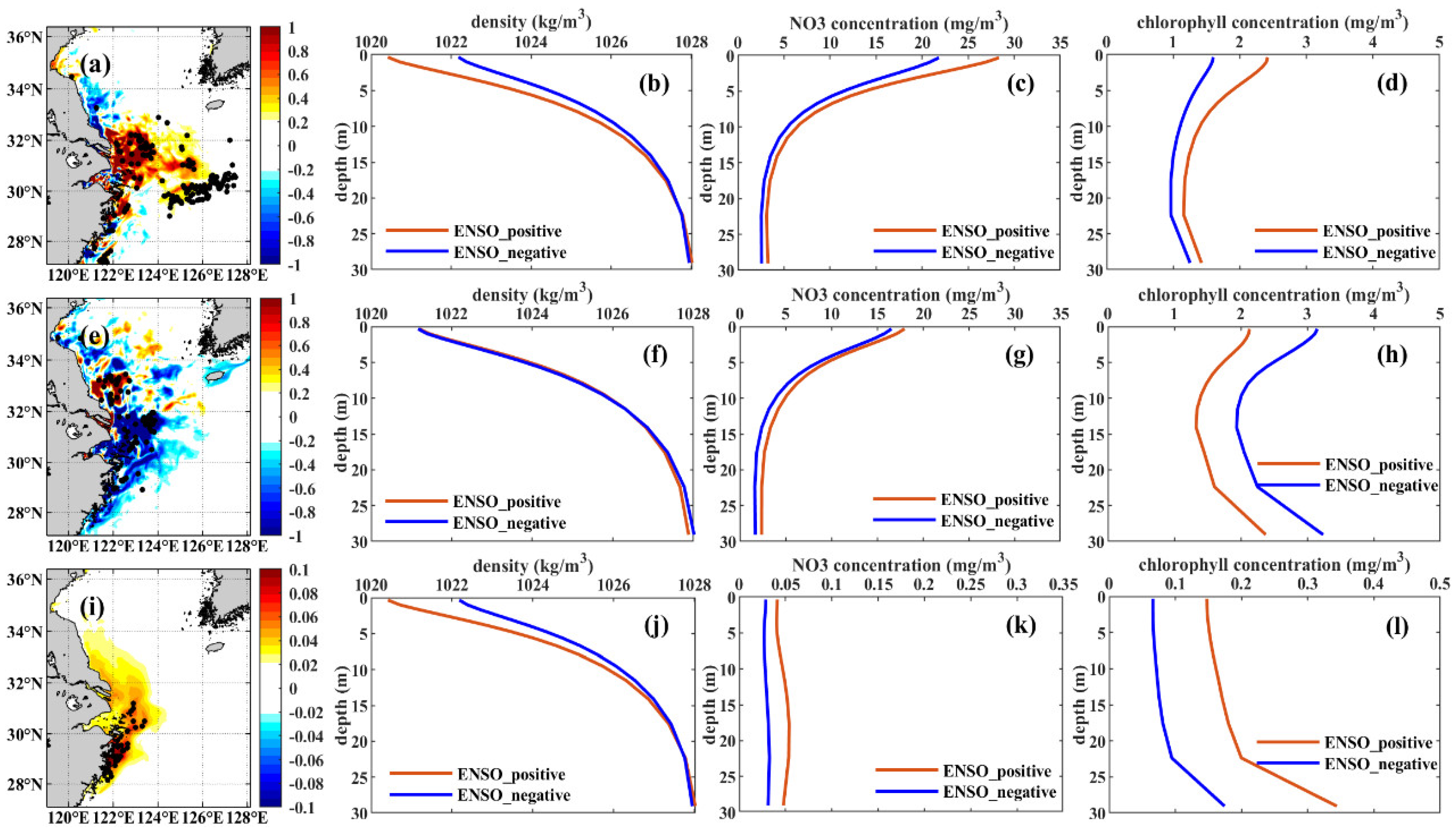
Nutrients are important factors influencing the growth process of phytoplankton [7,8,9,39]. Changjiang River discharge transports large amounts of nutrients into the estuary [3,4,5,6]. In order to study the chlorophyll concentration off the Changjiang River Estuary, freshwater discharge and nutrients were added to the ROMS-CoSiNE model. We use Gaussian-distributed precipitation around the estuary, which was converted by the discharge of the Changjiang River at a spatial scale, according to parameters related to the model resolution (60 km for the L1 domain, 120 km for the L0 domain) to present the freshwater discharge. This method has solved the problem of simulating complex estuary dynamics with coarse-resolution ocean models successfully [31,40,41,42,43]. Then, the nutrients carried by Changjiang River discharge were added to the ROMS-CoSiNE model. Three kinds of nutrients (nitrate, silicate, and phosphate) were added in the model, by multiplying the discharge with the observed nutrients concentration (nitrate: 41.9 mmol/m3 average from January 1963 to December 1999; silicate: 95.6 mmol/m3, and phosphate: 0.21 mmol/m3 average from January 1963 to December 1984) [4]. It was also assumed that the nutrients which were added to the model were mixed within 10 m below the sea surface [44]. In this way, we could convert the Changjiang River discharge (m3/s) into the rate of nutrient concentration change (unit: mmol/m3∙s), and add it as a source term for the nutrient temporal change.
This study performed three numerical experiments to investigate the influence of river discharge and riverine nutrients on chlorophyll concentration. The control experiment was referred to as Case 1, which was to add interannual variations of atmospheric and discharge forcing fields from 1998 to 2019. In Case 2, the discharge and nutrient concentration were fixed as the climatological annual cycle averaged from 1998 to 2019. In Case 3, interannual variation of discharge was considered in the model forcing. However, the nutrient concentration in the discharge was not included in the model. The atmospheric forcing fields except for freshwater discharge were the same for all three experiments. Table 1 lists more information about the three experiments.

3. Results

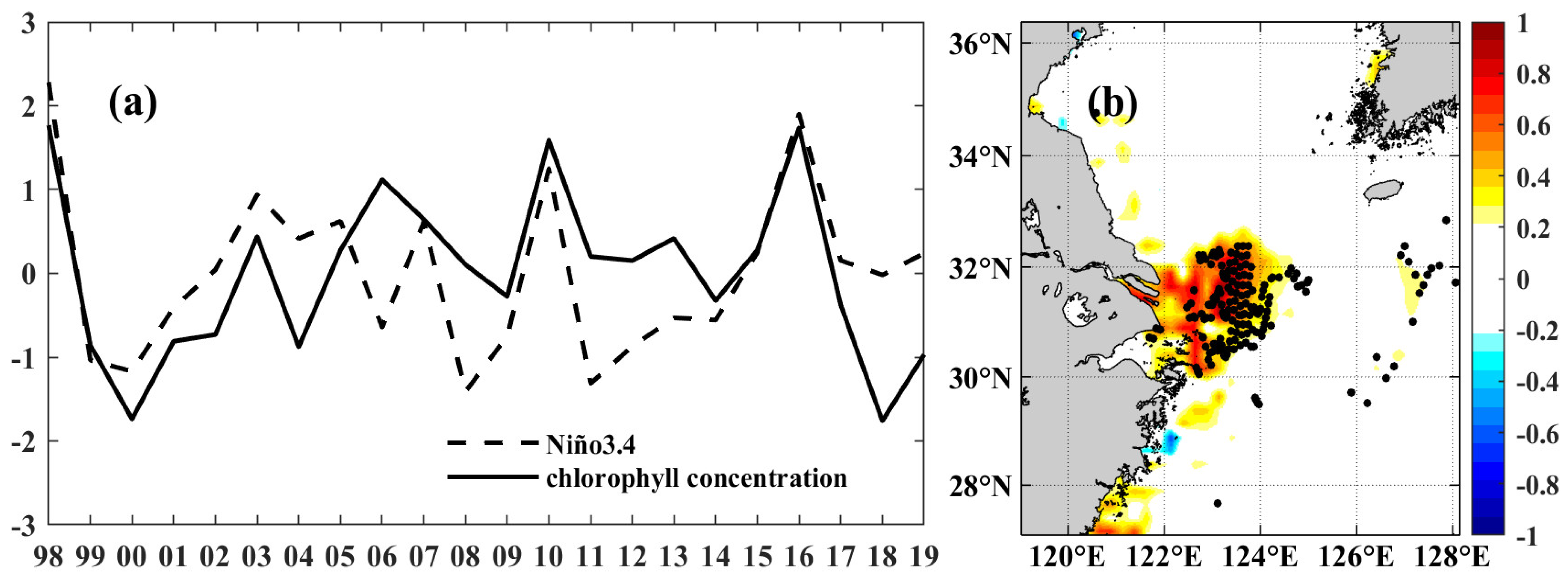
3.1. Interannual Variation of Chlorophyll Concentration off the Changjiang Estuary

As is well known, the high chlorophyll concentration in the Changjiang River Estuary emerges from spring to summer [45,46]. To illustrate the relationship between the chlorophyll concentration and ENSO, we showed the time series of the DJF-averaged Niño3.4 index from 1997 to 2019 and the AMJJA-averaged (April to August) chlorophyll concentration over the area 122.5°E–124°E, 30°N–32°N from the CCI (1998–2019) (Figure 2a). Interannual variability of the Niño3.4 index and chlorophyll concentration were highly consistent, especially during strong El Niño decay years (1998, 2010, and 2016. http://ggweather.com/enso/oni.htm, accessed on 1 January 2023). Chlorophyll concentration was significantly correlated with the Niño3.4 index with a correlation coefficient of 0.57 significant at the 95% confidence level. Figure 2b shows the composite differences in the spatial distribution of the chlorophyll concentration between the positive (1998, 2010, and 2016) and negative (1999, 2000, 2008, and 2011) ENSO phases. ENSO events were chosen based on a criterion of ± 1 standard deviation in our research, instead of the conventional 0.5 °C Niño3.4 SST anomalies using relatively strong El Niño and La Niña events. The chlorophyll concentration was positive over 122.5°E–124°E, 30°N–32°N with black dots representing the area significant at the 95% confidence level. The above analysis shows that the winter Niño3.4 index correlated well with the chlorophyll concentration off the Changjiang River Estuary for the following spring and summer.

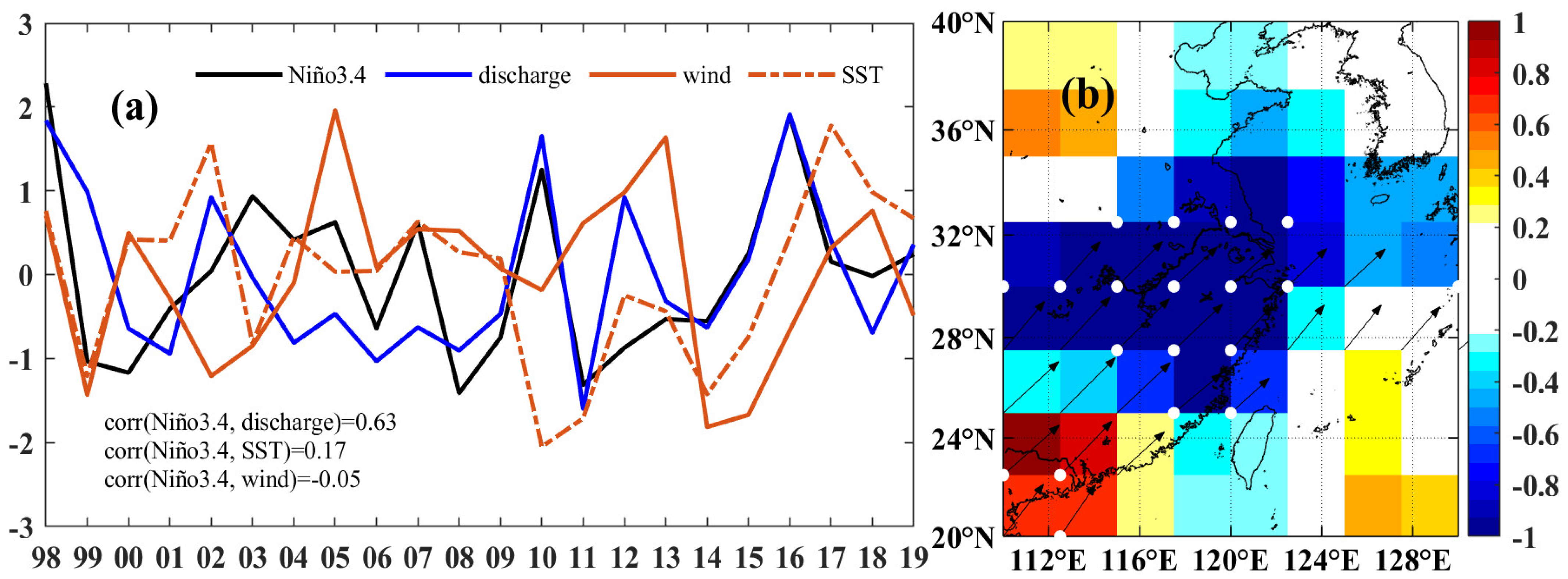
3.2. Possible Physical Mechanisms

Changes in the chlorophyll concentration may be linked to changes in the wind, SST, and coastal discharge over the coastal areas. The decreased wind speed would act to increase the stratification and reduce the nutrient exchange with deeper layers, thus reducing the chlorophyll concentration over the coastal areas [47]. The SST in the coastal area appreciably affected the chlorophyll concentration, exhibiting a positive correlation [48]. Changes in coastal discharge would result in changes in the nutrient concentration, and corresponding changes in the chlorophyll concentration over the coastal areas [12,49]. For our interannual analysis of the Changjiang River Estuary, these three variables may be responsible for the relationship between ENSO events and the coastal chlorophyll concentration. By calculating the correlation coefficients between the AMJJA-averaged discharge, SST, wind speed, and the DJF-averaged Niño3.4 from 1997 to 2019 (Figure 3a), we found that the discharge was significantly correlated with the Niño3.4 index with a correlation coefficient of 0.63 significant at the 99% confidence level. Both the SST and wind speed were averaged over the focus area 122.5°E–124°E, 30°N–32°N from April to August of each year. This result reached the same conclusion as Jiang et al. [50] and Zhang et al. [51], who showed that high levels of the Changjiang River discharge generally occurred in warm ENSO phases, and low discharge levels occurred in cold phases. The correlation coefficients between SST, wind speed, and DJF-averaged Niño3.4 were 0.17 and −0.05, respectively, which were not significant at the 95% confidence level. The above linear analysis shows that the Niño3.4 index for the winter is a good predictor for the discharge in the following spring and summer. Figure 3b shows the regressed 850 hPa water vapor flux and 850 hPa vapor flux divergence upon the previous winter DJF-averaged Niño3.4 index. The middle and lower reaches of the Changjiang River had southerly wind anomaly and water vapor flux convergence, which is associated with more precipitation and therefore more discharge [52,53,54]. Estuary nutrients mainly come from discharge and change with discharge volume [55,56]. Thus, ENSO events can cause the change of the Changjiang River discharge which is critical to the nutrient supply of the estuary marine environment.
The regressed chlorophyll concentration upon the AMJJA-averaged discharge from 1998 to 2019 indicated that the chlorophyll concentration was positively correlated with discharge off the estuary, especially around our focus area of 122.5°E–124°E, 30°N–32°N (Figure 4a). The interannual variation of the chlorophyll concentration was positively correlated with the discharge, indicating that the chlorophyll concentration may be affected by the discharge off the estuary, especially over the area of 122.5°E–124°E, 30°N–32°N, which is consistent with Chen et al. [11] and Wang et al. [12]. The discharge was significantly correlated with the averaged chlorophyll concentration in the focus area 122.5°E–124°E, 30°N–32°N with a correlation coefficient of 0.44 significant at the 95% confidence level (Figure 4b). Discharge took the lead role in affecting the chlorophyll concentration in the focus area, especially in high discharge years (1998, 2010 and 2016). The above analysis shows that the interannual variation of chlorophyll concentration in 122.5°E–124°E, 30°N–32°N is not completely affected by the interannual variation in discharge, but that the discharge is still the main factor affecting the chlorophyll concentration in high discharge years.

4. Model Results

With the influence of meteorological and oceanic factors, the riverine discharge will spread from the estuary and the variable discharge itself cannot represent the spread of discharge off the Changjiang River estuary [57,58]. On the other hand, the SSS can represent the expansion of freshwater (Wu et al. [59]). The SSS was used to analyze the cause of the abnormal spatial distribution of chlorophyll concentration during the ENSO years. The two-level nested ROMS-CoSiNE coupled model presented in Section 2 was used to investigate the relationship between the discharge and chlorophyll concentration during the ENSO years.

4.1. Validation of Model Simulation

The model simulation was first validated against observation using output from the control integration Case 1 in which the Changjiang River discharge and associated nutrients were included. Figure 5 shows that the composite differences of SST, SSS, and density had similar special distributions in observation (Figure 5a–c) and model output (Figure 5d–f). The composite differences of SST from the observation (Figure 5a) and model (Figure 5d) had positive SST anomaly east of 126°E, away from the Changjiang River Estuary. The composite differences of both SSS (Figure 5b,c) and density (Figure 5c,f) represented negative anomalies off the Changjiang River Estuary, indicating the spread of freshwater discharge. There were subtle differences between the model and observation. In the observation (Figure 5b,c), the spread of freshwater discharge was further extended toward the northeast direction. In the model output (Figure 5e,f), the freshwater discharge was confined off the Changjiang River Estuary, and caused larger negative SSS and density anomaly than that in the observation. Overall, the model can reproduce the spread of freshwater discharge of the Changjiang River and SSS, and density differences between the ENSO-positive and -negative phase years. In the later sections, the outputs from the two sensitivity experiments were used to quantify the influence of the discharge and nutrients carried by the discharge.
After the discharge enters the ocean, the nutrients carried by the river discharge can enhance the phytoplankton growth and increase the chlorophyll concentration. Figure 6a shows the correlation coefficient distribution between the AMJJA-averaged chlorophyll concentration of CCI and the AMJJA-averaged SSS of observation from 1998 to 2019. The correlation coefficient was negative, and significant at the 95% confidence level off the Changjiang River Estuary. The distribution of the correlation coefficient between the SSS and chlorophyll concentration was consistent with the abnormal distribution of chlorophyll concentration during the ENSO years off the Changjiang River Estuary (Figure 2b), indicating the above normal discharge from the Changjiang River spreading at the surface of the estuary in positive ENSO years and bringing more nutrients to the surface. Therefore, the chlorophyll concentration in the ENSO-positive years was higher than that in the negative ENSO years. The averaged SSS and chlorophyll concentration of the focus area had a correlation coefficient of −0.62 significant at the 95% confidence level. The ROMS-CoSiNE model showed the same spatial distribution of correlation coefficient between SSS and chlorophyll concentration (Figure 6c) as the observation (Figure 6a), and the SSS was also significantly correlated with the chlorophyll concentration with a correlation coefficient of −0.66 significant at the 95% confidence level (Figure 6d). This indicates that the model can reproduce the relationship between SSS and chlorophyll concentration.

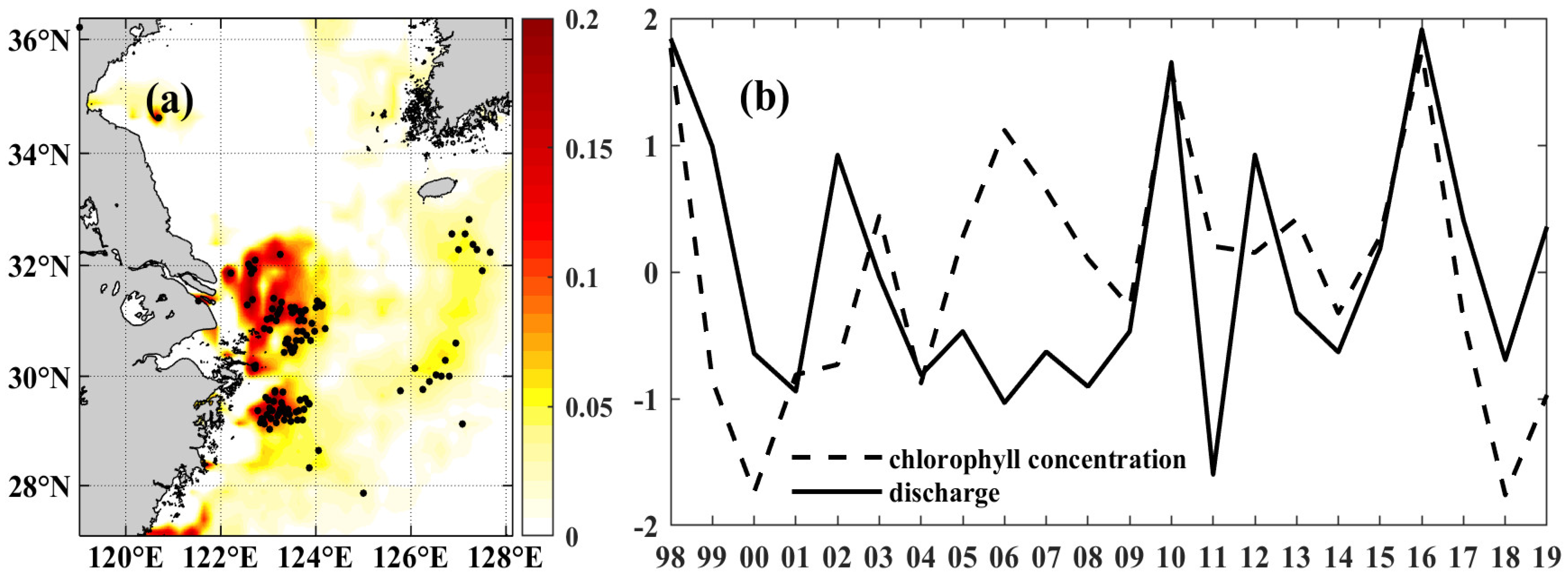
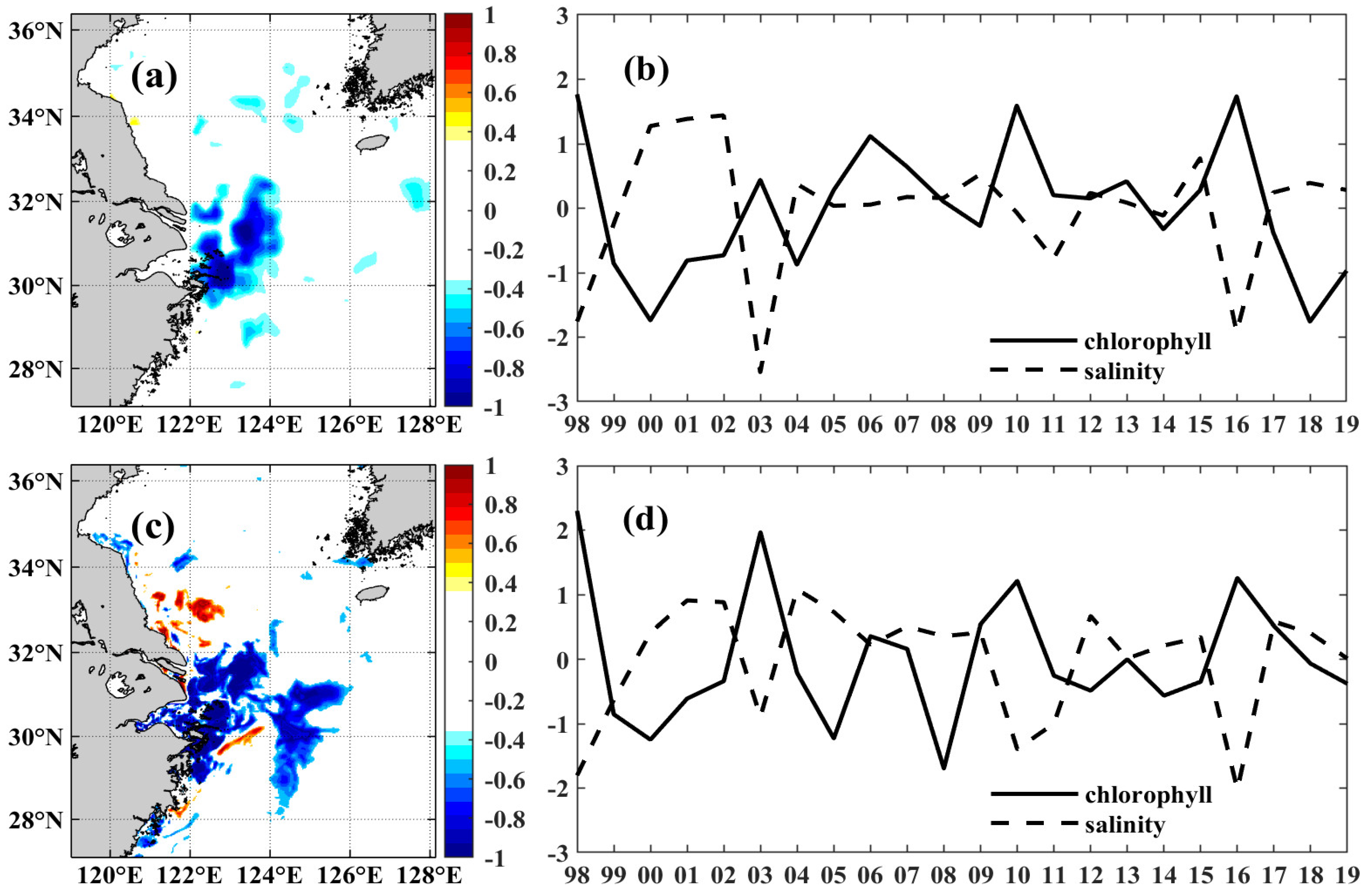
4.2. The Influence of Discharge and Nutrients on Chlorophyll Concentration

As discussed in Section 3.2, the change in wind forcing, ocean temperature and discharge all can cause changes in chlorophyll concentration in coastal waters. To identify the mechanism of chlorophyll concentration changes in the Changjiang River Estuary, two sensitivity numerical experiments were conducted (Table 1). In Case 2, the discharge and nutrients carried by the discharge were fixed as a constant seasonal cycle which was the average from 1998 to 2019. In Case 3, only the interannual variation of discharge was considered. However, there were no nutrients in the discharge.
Figure 7 compares these two experiments against the control integration of Case 1. In all three experiments, other atmospheric forcing fields were kept the same. From Figure 7a, the composite difference of the model chlorophyll concentration between ENSO-positive and ENSO-negative phase years indicated an enhanced chlorophyll concentration off the Changjiang River Estuary, which bore a similar spatial pattern as that of the observation (Figure 2b). In the study area 122.5°E–124°E, 30°N–32°N, the density was reduced (Figure 7b), the NO3 concentration was enhanced (Figure 7c), and the chlorophyll concentration in the water column was enhanced (Figure 7d) in the ENSO-positive phase years. If the discharge and nutrients were fixed as a constant seasonal cycle, the chlorophyll concentration was reduced in the ENSO-positive phase years (Figure 7e,h), without obvious changes in density (Figure 7f) and NO3 concentration (Figure 7g). This reflects the important role of discharge in causing chlorophyll concentration variation. If the discharge force was considered and there were no nutrients in the discharge, the model could reproduce the density reduction in the ENSO-positive phase years (Figure 7j), and an enhanced chlorophyll concentration (Figure 7i,c) which was one order of magnitude smaller than that in Case 1 and the observation. Comparing Figure 7c,g,k, we can conclude that the nutrients from the Changjiang River play a dominant role in the Changjiang River Estuary. Without the nutrients carried by the river discharge, the NO3 concentration would be reduced by one order to two orders of magnitude. Though river discharge can reproduce the stratification change in ENSO-positive phase years, it is the nutrients transported by the discharge that cause the chlorophyll concentration change.

5. Discussions and Conclusions

The April to August averaged chlorophyll concentration from the CCI product over the focus area 122.5°E–124°E, 30°N–32°N was significantly correlated with the December to February averaged Niño3.4 index from the previous winter from 1998 to 2019. Among the three variables (10 m winds, SST, and discharge) that may reflect the interaction between ENSO and the chlorophyll concentration in coastal areas, only the discharge was significantly correlated with the previous winter’s Niño3.4 index. When studying the relationship between the discharge and chlorophyll concentration off the Changjiang River Estuary, we found that the chlorophyll concentration was mainly affected by the discharge in high discharge years. To address the question of the impact of the Changjiang River discharge on the nearshore marine ecosystem, we can study the flow area of the discharge by analyzing the spatial distribution characteristic of the SSS on the interannual time scale. Therefore, it is possible that the chlorophyll concentration off the Changjiang River Estuary may be related to the interannual variation of the SSS. However, for the relationship between the discharge and nutrients, we can only analyze its impact on the estuarine ecosystem with the help of a numerical model due to the lack of continuous temporal and spatial scale observations of nutrients.
A two-level nested ROMS-CoSiNE coupled model was used to study the impact of discharge and nutrients carried by the discharge on the chlorophyll concentration during the ENSO years off the Changjiang River Estuary. The model could reproduce the spatial distributions of SST, SSS, and density anomaly and the relationship between the SSS and chlorophyll concentration during the ENSO years off the Changjiang River Estuary. We have studied the relationship between the Changjiang River discharge and SSS, and chlorophyll concentration. Therefore, when changing the interannual variation of discharge and nutrients carried by the discharge, it must be considered whether the chlorophyll concentration would also change interannually. Based on this, we designed a sensitivity experiment in the model to illustrate this question. When the discharge and nutrients carried by the discharge were fixed as a constant seasonal cycle, the chlorophyll concentration in the Changjiang River Estuary was reduced in ENSO-positive phase years.
The contribution of nutrients carried by the Changjiang River discharge in relation to the chlorophyll concentration off the Changjiang River Estuary was also considered. When removing nutrients from the discharge, the nutrient concentration in the Changjiang River Estuary was reduced by one to two orders of magnitude and the interannual variation of chlorophyll concentration was also reduced by one order of magnitude. By comparing the outputs from the control experiment with the two sensitivity experiments, it may be concluded that the freshwater discharge can modify the stratification, and it is the nutrients carried by the discharge that play a dominant role in causing the chlorophyll concentration variation associated with the ENSO-positive and -negative phase years.

Author Contributions

Investigation, resources, methodology, writing original draft, conceptualization, validation, methodology, analysis, project administration, Q.W.; writing, editing, investigation, funding acquisition, review, X.W.; investigation, editing, Y.H. and J.Z.; All authors have read and agreed to the published version of the manuscript.

Funding

This study was supported by the National Key Research and Development Program (2016YFC1401600), Key Laboratory of Research on Marine Hazards Forecasting Open Fund (LOMF2203) and China Scholarship Council (201908320507).

Data Availability Statement

Freshwater discharge data from 1998 to 2019 are downloaded from the Datong hydrological station (http://xxfb.hydroinfo.gov.cn, accessed on 20 October 2022). The monthly Niño3.4 index from 1997 to 2019 is downloaded from the National Oceanic & Atmospheric Administration’s website (https://www.esrl.noaa.gov/psd/data/correlation/nina34.data, accessed on 1 January 2023). The monthly chlorophyll concentration observation data is from the 4.2 version of the CCI dataset (1998–2019, https://esa-oceancolour-cci.org/, accessed on 1 January 2023). Monthly 10 m wind data is drawn from fifth-generation ECMWF reanalysis data (ERA5 dataset) and is downloaded from http://apdrc.soest.hawaii.edu/data/data.php (accessed on 1 January 2023). The monthly global marine temperature and salinity grid data products are from the marine science data center of the Chinese Academy of Sciences (http://msdc.qdio.ac.cn/data/metadata-special, accessed on 1 January 2023).

Acknowledgments

Thanks for the temperature and salinity data service provided by the Oceanographic Data Center, Chinese Academy of Sciences (CASODC) (http://msdc.qdio.ac.cn, accessed on 3 March 2023), and thank the anonymous reviewers for their constructive and thoughtful comments.

Conflicts of Interest

The authors declare no conflict of interest.

References

  1. Zhang, J.; Liu, S.M.; Ren, J.L. Nutrients gradients from the eutrophic Changjiang (Yangtze River) estuary to the oligotrophic Kuroshio Waters and re-evaluation of budgets for the East China Sea shelf. Prog. Oceanogr. 2007, 74, 449–478. [Google Scholar] [CrossRef]
  2. Liu, K.K.; Gong, G.C.; Wu, C.R. The Kuroshio and the East China Sea. In Carbon and Nutrients Fluxes in Continental Margins: A Global Synthesis; Liu, K.K., Atkinson, L., Quiñones, R., Talaue-McManus, L., Eds.; IGBP Book Series; Springer: Berlin/Heidelberg, Germany, 2010; pp. 124–146. [Google Scholar]
  3. Zhang, J. Nutrients elements in large Chinese estuaries. Cont. Shelf Res. 1996, 16, 1023–1045. [Google Scholar] [CrossRef]
  4. Liu, X.C.; Shen, H.T.; Huang, Q.H. Concentration variation and flux estimation of dissolved inorganic nutrients from the Changjiang River into its estuary. Oceanol. Limnol. Sin. 2002, 33, 332–340. Available online: https://en.cnki.com.cn/Article_en/CJFDTOTAL-HYFZ200203013.htm (accessed on 2 January 2023).
  5. Shen, Z.L.; Liu, Q. Nutrients in the Changjiang River. Environ. Monit Assess 2009, 153, 27–44. [Google Scholar] [CrossRef]
  6. Chai, C.; Yu, Z.M.; Shen, Z.L. Nutrients characteristics in the Yangtze River Estuary and the adjacent East China Sea before and after impoundment of the Three Gorges Dam. Sci. Total Environ. 2009, 407, 4687–4695. [Google Scholar] [CrossRef] [PubMed]
  7. Domingues, R.B.; Barbosa, A.; Galvão, H. Nutrients, light and phytoplankton succession in a temperate estuary (the Guadiana, south-western Iberia) Estuarine. Estuar. Coast. Shelf Sci. 2005, 64, 249–260. [Google Scholar] [CrossRef]
  8. Furnas, M.; Mitchell, A.; Skuza, M. In the other 90%: Phytoplankton responses to enhanced nutrients availability in the Great Barrier Reef Lagoon. Mar. Pollut. Bull. 2005, 51, 253–265. [Google Scholar] [CrossRef] [PubMed]
  9. Paerl, H.W. Assessing and managing nutrients-enhanced eutrophication in estuarine and coastal waters: Interactive effects of human and climatic perturbations. Ecol. Eng. 2006, 26, 40–54. [Google Scholar] [CrossRef]
  10. Gong, G.C.; Liu, K.K.; Pai, S.C. Prediction of nitrate concentration from two end member mixing in the southern East China Sea. Cont. Shelf Res. 1995, 15, 827–842. [Google Scholar] [CrossRef]
  11. Chen Lee, Y.L.; Chen, H.Y.; Gong, G.C. Phytoplankton production during a summer coastal upwelling in the East China Sea. Cont. Shelf Res. 2004, 24, 1321–1338. [Google Scholar] [CrossRef]
  12. Wang, Y.; Jiang, H.; Jin, J.X. Spatial-Temporal Variations of Chlorophyll in the Adjacent Sea Area of the Yangtze River Estuary Influenced by Yangtze River Discharge. Int. J. Environ. Res. Public Health 2015, 12, 5420–5438. [Google Scholar] [CrossRef] [PubMed]
  13. Zhou, M.J.; Yan, T.; Zou, J.Z. Preliminary analysis of the characteristics of red tide areas in Changjiang River Estuary and its adjacent sea. Chin. J. Appl. Ecol. 2003, 14, 1031–1038. Available online: https://pubmed.ncbi.nlm.nih.gov/14587317/ (accessed on 1 January 2023).
  14. Zhou, M.J.; Zhu, M.Y. Progress of the project “Ecology and oceanography of harmful algal blooms in China”. Adv. Earth Sci. 2006, 21, 673–679. [Google Scholar]
  15. Zhou, M.J.; Shen, Z.L.; Yu, R.C. Responses of a coastal phytoplankton community to increased nutrients input from the Changjiang (Yangtze) River. Cont. Shelf Res. 2008, 28, 1483–1489. [Google Scholar] [CrossRef]
  16. Hu, D.X. Some striking features of circulation in Huanghai Sea and East China Sea. Oceanol. China Seas 1994, 11, 27–28. [Google Scholar] [CrossRef]
  17. Isobe, A.; Ando, M.; Watanabe, T. Freshwater and temperature transports through the Tsushima–Korea Straits. J. Geophys. Res. 2002, 107, 3065. [Google Scholar] [CrossRef]
  18. Lie, H.J.; Cho, C.H.; Lee, J.H. Structure and eastward extension of the Changjiang River plume in the East China Sea. J. Geophys. Res. 2003, 108, 3077. [Google Scholar] [CrossRef]
  19. Liu, X.Y.; Liu, Y.G.; Guo, L. Interannual changes of sea level in the two regions of East China Sea and different responses to ENSO. Global Planet. Change 2010, 72, 215–226. [Google Scholar] [CrossRef]
  20. Park, T.; Jang, C.J.; Kwon, M. An effect of ENSO on summer surface salinity in the Yellow and East China seas. J. Mar. Syst. 2015, 141, 122–127. [Google Scholar] [CrossRef]
  21. Gong, G.G.; Wen, Y.H.; Wang, B.W. Seasonal variation of chlorophyll a concentration, primary production and environmental conditions in the subtropical East China Sea. Deep. Sea Res. Part II Top. Stud. Oceanogr. 2003, 50, 1219–1236. [Google Scholar] [CrossRef]
  22. He, X.Q.; Bai, Y.; Pan, D.L. Satellite views of the seasonal and interannual variability of phytoplankton blooms in the eastern China seas over the past 14 yr (1998–2011). Biogeosciences 2013, 10, 4721–4739. [Google Scholar] [CrossRef]
  23. Hallegraeff, G.M. Ocean climate change, phytoplankton community responses, and harmful algal blooms: A formidable predictive challenge. J. Phycol. 2010, 46, 220–235. [Google Scholar] [CrossRef]
  24. Stramska, M. Interannual variability of seasonal phytoplankton blooms in the north polar Atlantic in response to atmospheric forcing. J. Geophys. Res. C Oceans 2005, 110, C05016-1. [Google Scholar] [CrossRef]
  25. Chai, F.; Lindley, S.T.; Barber, R.T. Origin and maintenance of a high NO3 condition in the equatorial Pacific. Deep. Sea Res. Part II Top. Stud. Oceanogr. 1996, 43, 1031–1064. [Google Scholar] [CrossRef]
  26. Chai, F.; Dugdale, R.C.; Peng, T.H. One-dimensional ecosystem model of the equatorial Pacific upwelling system. Part I: Model development and silicon and nitrogen cycle. Deep. Sea Res. Part II Top. Stud. Oceanogr. 2002, 49, 2713–2745. [Google Scholar] [CrossRef]
  27. Xiu, P.; Chai, F. Modeled biogeochemical responses to mesoscale eddies in the South China. J. Geophys. Res. C Oceans 2011, 116, C10. [Google Scholar] [CrossRef]
  28. Xiu, P.; Chai, F. Spatial and temporal variability in phytoplankton carbon, chlorophyll, and nitrogen in the North Pacific. J. Geophys. Res. C Oceans 2012, 117, C11023. [Google Scholar] [CrossRef]
  29. Xiu, P.; Chai, F. Connections between physical, optical and biogeochemical processes in the Pacific Ocean. Prog. Oceanogr. 2014, 122, 30–53. [Google Scholar] [CrossRef]
  30. Zhou, F.; Chai, F.; Huang, D.J. Investigation of hypoxia off the Changjiang Estuary using a coupled model of ROMS-CoSiNE. Prog. Oceanogr. 2017, 159, 237–254. [Google Scholar] [CrossRef]
  31. Wu, Q.; Wang, X.C.; Xiu, P. Sensitivity of chlorophyll variability to specific growth rate of phytoplankton over the Yangtze River estuary in a physical-biogeochemical model. Atmosphere 2022, 13, 1748. [Google Scholar] [CrossRef]
  32. Garcia, H.E.; Locarnini, R.A.; Boyer, T.P. World Ocean Atlas 2005, Nutrients (Phosphate, Nitrate, Silicate); Government Printing Office: Washington, DC, USA, 2006; pp. 2–14. Available online: https://repository.library.noaa.gov/view/noaa/1129 (accessed on 1 January 2023).
  33. Kalnay, E.; Kanamitsu, M.; Kistler, R. The NCEP/NCAR 40-year reanalysis project. Bull. Am. Meteorol. Soc. 1996, 77, 437–471. [Google Scholar] [CrossRef]
  34. Kondo, J. Air-sea bulk transfer coefficients in diabatic conditions. Bound. Layer Meteorol. 1975, 9, 91–112. [Google Scholar] [CrossRef]
  35. Large, W.G.; Pond, S. Sensible and latent heat flux measurements over the ocean. J. Phys. Oceanogr. 1982, 12, 464–482. [Google Scholar] [CrossRef]
  36. Key, R.M.; Kozyr, A.; Sabine, C.L. A global ocean carbon climatology: Results from GLODAP. Global Biogeochem. Cycles 2004, 18, GB4031. [Google Scholar] [CrossRef]
  37. Cheng, L.J.; Trenberth, K.E.; Fasullo, J. Improved estimates of ocean heat content from 1960 to 2015. Sci. Adv. 2017, 3, e1601545. [Google Scholar] [CrossRef] [PubMed]
  38. Cheng, L.J.; Trenberth, K.E.; Gruber, N. Improved estimates of changes in upper ocean salinity and the hydrological cycle. J. Clim. 2020, 33, 10357–10381. [Google Scholar] [CrossRef]
  39. Luo, B.Z.; Liu, R.Y. Construction of Three Gorge Dam Project and the Ecology and Environment in the Estuary Science Press; Beijing Publication: Beijing, China, 1994; p. 343. [Google Scholar]
  40. Berdeal, I.B.; Hickey, B.M.; Kawase, M. Influence of wind stress and ambient flow on a high discharge river plume. J. Geophys. Res. C Oceans 2002, 107, 3130. [Google Scholar] [CrossRef]
  41. Jin, M.B.; Wang, J. Interannual variability and sensitivity study of the ocean circulation and thermohaline structure in Prince William Sound, Alaska. Cont. Shelf Res. 2004, 24, 393–411. [Google Scholar] [CrossRef]
  42. Mooers, C.N.K.; Wu, X.L.; Bang, I. Performance of a nowcast/forcast system for Prince William Sound, Alaska. Cont. Shelf Res. 2007, 29, 42–60. [Google Scholar] [CrossRef]
  43. Wang, X.C.; Chao, Y.; Zhang, H.C. Modeling tides and their influence on the circulation in Prince William Sound, Alaska. Cont. Shelf Res. 2013, 63, S126–S137. [Google Scholar] [CrossRef]
  44. Chang, P.H.; Isobe, A. A numerical study on the Changjiang diluted water in the Yellow and East China Seas. J. Geophys. Res. Oceans 2003, 108, C9. [Google Scholar] [CrossRef]
  45. Ye, S.F.; Ji, H.H.; Cao, L. Red tides in the Yangtze River Estuary and adjacent sea areas: Causes and mitigation. Mar. Sci. 2002, 28, 26–32. [Google Scholar]
  46. Chen, C.S.; Zhu, J.R.; Beardsley, R.C. Physical-biological sources for dense algal blooms near the Changjiang River. Geophys. Res. Lett. 2003, 30, 1515. [Google Scholar] [CrossRef]
  47. Gregg, W.W.; Casey, N.W.; McClain, C.R. Recent trends in global ocean chlorophyll. Geophys. Res. Lett. 2005, 32, L03606. [Google Scholar] [CrossRef]
  48. Ji, C.X.; Zhang, Y.Z.; Cheng, Q.M. Evaluating the impact of sea surface temperature (SST) on spatial distribution of chlorophyll-a concentration in the East China Sea. Int. J. Appl. Earth Obs. Geoinf. 2018, 68, 252–261. [Google Scholar] [CrossRef]
  49. Ware, D.M.; Thomson, R.E. Bottom-up ecosystem trophic dynamics determine fish production in the Northeast Pacific. Science 2005, 308, 1280–1284. [Google Scholar] [CrossRef]
  50. Jiang, T.; Zhang, Q.; Zhu, D.M. Yangtze floods and droughts (China) and teleconnections with ENSO activities (1470–2003). Quatern. Int. 2006, 144, 29–37. [Google Scholar] [CrossRef]
  51. Zhang, Q.; Yu, C.Y.; Jiang, T. Possible influences of ENSO on annual maximum streamflow of the Yangtze River, China. J. Hydrol. 2007, 333, 265–274. [Google Scholar] [CrossRef]
  52. Chen, J.; Wu, X.; Finlayson, B.L. Variability and trend in the hydrology of the Yangtze River, China: Annual precipitation and runoff. J. Hydrol. 2014, 513, 403–412. [Google Scholar] [CrossRef]
  53. Wang, B.; Li, J.; He, Q. Variable and robust East Asian monsoon rainfall response to El Niño over the past 60 years (1957–2016). Adv. Atmos. Sci. 2017, 34, 1235–1248. [Google Scholar] [CrossRef]
  54. Li, T.; Wang, B.; Wu, B. Theories on Formation of an Anomalous Anticyclone in Western North Pacific during El Niño: A Review. J. Meteorol. Res. 2017, 31, 987–1006. [Google Scholar] [CrossRef]
  55. Shen, Z.L. A study on the relationships of the nutrients near the Changjiang river estuary with the flow of the Changjiang river water. Chin. J. Oceanol. Limnol. 1993, 11, 260–267. Available online: http://www.cnki.com.cn/Article/CJFDTotal-HYFW199303008.htm (accessed on 1 January 2023).
  56. Wang, K.; Chen, J.F.; Jin, H.Y. The four seasons nutrients distribution in Changjiang River Estuary and its adjacent East China Sea. J. Mar. Sci. 2011, 29, 18–35. Available online: http://en.cnki.com.cn/Article_en/CJFDTOTAL-DHHY201103005.htm (accessed on 1 January 2023).
  57. Cloern, J.E. Phytoplankton bloom dynamics in coastal ecosystems: A review with some general lessons from sustained investigation of San Francisco Bay, California. Rev. Geophys. 1996, 34, 127–168. [Google Scholar] [CrossRef]
  58. Yin, K.D.; Zhang, J.L.; Qian, P.Y. Effect of wind events on phytoplankton blooms in the Pearl River estuary during summer. Cont. Shelf Res. 2004, 24, 1909–1923. [Google Scholar] [CrossRef]
  59. Wu, Q.; Wang, X.C.; Liang, W.H. Validation and application of soil moisture active passive sea surface salinity observation over the Changjiang River Estuary. Acta Oceanol. Sin. 2020, 39, 1–8. [Google Scholar] [CrossRef]
Figure 1. (a) The outer model domain (L0) covers the entire Chinese coast. The black rectangle denotes the second domain (27°N–36°N, 119°E–128°E). (b) The second model domain (L1) covers the entire Changjiang River Estuary. The black rectangle here denotes the focus area (122.5°E–124°E, 30°N–32°N) of our time series analysis. The Bathymetry of the model domain is shown in meters.
Remotesensing 15 02384 g001
Figure 2. (a) The AMJJA-averaged standardized chlorophyll concentration based on CCI from 1998 to 2019 for 122.5°E–124°E, 30°N–32°N and the Niño3.4 index for the previous winter. (b) Composite differences in chlorophyll concentration between positive and negative ENSO phases (ENSO events were chosen based on a criterion of ± 1 standard deviation). The black dot indicates regions that were significant at the 95% level based on Student’s t-test.
Remotesensing 15 02384 g002
Figure 3. (a) Time series of AMJJA-averaged standardized discharge, 10 m wind speed, and SST from 1998 to 2019 and DJF-averaged standardized Niño3.4 index for the previous winter. Both the SST and wind speed were averaged over the focus area 122.5°E–124°E, 30°N–32°N and from April to August of each year. (b) The 850 hPa water vapor flux and 850 hPa water vapor flux divergence regressed onto the Niño3.4 index. Black arrows and white dots are significant at the 95% confidence level. Water vapor transport flux is in kg/(m · s), and water vapor flux divergence is in 105 kg/(m2 s).
Remotesensing 15 02384 g003
Figure 4. (a) The AMJJA-averaged chlorophyll concentration from the CCI regressed onto the discharge from 1998 to 2019 (shade), and the significant correlation coefficient distribution between discharge and chlorophyll concentration (black dots). (b) The time series of AMJJA-averaged standardized chlorophyll concentration for the focus area 122.5°E–124°E, 30°N–32°N and discharge from 1998 to 2019.
Remotesensing 15 02384 g004
Figure 5. (a) Composite differences in SST between positive and negative ENSO phases (ENSO events were chosen based on a criterion of ± 1 standard deviation); (b) the same as (a) but for SSS. (c) the same as (a) but for density. (df) the same as (ac) but for model results. The black dots indicate regions where the difference was significant at the 95% confidence level based on Student’s t-test. The unit for SST is °C, the unit for SSS is PSU, and the unit for density is kg/m3.
Remotesensing 15 02384 g005
Figure 6. (a) The correlation coefficient distribution between AMJJA-averaged chlorophyll concentration and AMJJA-averaged SSS (shade) from 1998 to 2019. (b) The time series of AMJJA-averaged standardized chlorophyll concentration for 122.5°E–124°E, 30°N–32°N and SSS from 1998 to 2019. (c) the same as (a) but for model result. (d) the same as (b) but for model result. The shade is where the correlation coefficient was significant at the 95% confidence level.
Remotesensing 15 02384 g006
Figure 7. (a) Composite differences of simulated chlorophyll concentration from Case 1 which includes interannual variations in discharge and nutrients between positive and negative ENSO phases (ENSO events were chosen based on a criterion of ± 1 standard deviation). The unit for chlorophyll concentration is mg/m3. (b) The density profiles averaged over 122.5°E–124°E, 30°N–32°N for positive and negative ENSO phases. The unit for density is kg/m3. (c) the same as (b) but for NO3. The unit for NO3 is mg/m3. (d) the same as (b) but for chlorophyll concentration. The unit for chlorophyll concentration is mg/m3. (e) Composite differences of modeled chlorophyll concentration between positive and negative ENSO phases from Case 2 with discharge and nutrients taken as a fixed seasonal cycle. (f) the same as (b) but for Case 2. (g) the same as (c) but for Case 2. (h) the same as (d) but for Case 2. (i) Composite differences in chlorophyll concentration from Case 3 with only interannual variation in discharge but no nutrients in discharge for positive and negative ENSO phases. (j) the same as (b) but for Case 3. (k) the same as (c) but for Case 3. (l) the same as (d) but for Case 3. The black dots indicate regions that were significant at 95% confidence level based on Student’s t-test.
Remotesensing 15 02384 g007
Table 1. Details of the three experiments.
Forcing and Boundary ConditionsDischarge and Nutrients
Case 1Year-to-year variationYear-to-year variation
Case 2Year-to-year variationAnnual cycle (1998–2019 averaged)
Case 3Year-to-year variationYear-to-year variationof discharge
The integration period was from 1998 to 2019.
Disclaimer/Publisher’s Note: The statements, opinions and data contained in all publications are solely those of the individual author(s) and contributor(s) and not of MDPI and/or the editor(s). MDPI and/or the editor(s) disclaim responsibility for any injury to people or property resulting from any ideas, methods, instructions or products referred to in the content.

