Spectral Correlation and Spatial High–Low Frequency Information of Hyperspectral Image Super-Resolution Network

Abstract

Hyperspectral images (HSIs) generally contain tens or even hundreds of spectral segments within a specific frequency range. Due to the limitations and cost of imaging sensors, HSIs often trade spatial resolution for finer band resolution. To compensate for the loss of spatial resolution and maintain a balance between space and spectrum, existing algorithms were used to obtain excellent results. However, these algorithms could not fully mine the coupling relationship between the spectral domain and spatial domain of HSIs. In this study, we presented a spectral correlation and spatial high–low frequency information of a hyperspectral image super-resolution network (SCSFINet) based on the spectrum-guided attention for analyzing the information already obtained from HSIs. The core of our algorithms was the spectral and spatial feature extraction module (SSFM), consisting of two key elements: (a) spectrum-guided attention fusion (SGAF) using SGSA/SGCA and CFJSF to extract spectral–spatial and spectral–channel joint feature attention, and (b) high- and low-frequency separated multi-level feature fusion (FSMFF) for fusing the multi-level information. In the final stage of upsampling, we proposed the channel grouping and fusion (CGF) module, which can group feature channels and extract and merge features within and between groups to further refine the features and provide finer feature details for sub-pixel convolution. The test on the three general hyperspectral datasets, compared to the existing hyperspectral super-resolution algorithms, suggested the advantage of our method.

1. Introduction

Hyperspectral images (HSIs) based on remote sensing satellites have a large amount of narrowband information, generated by combining imaging technology and spectral technology. HSIs contain two-dimensional geometric space and one-dimensional spectral information on the target. They are carefully segmented in the spectral dimension, not only the traditional black, white, or RGB differences, but also N channels in the spectral dimension. HSIs are used in many areas, such as land monitoring [1,2], urban planning [3], road network layout [4], agricultural yield estimation [5], and disaster prevention and control [6]. Hyperspectral technology is characterized by a multiband, narrow spectral range, continuous band, and a large amount of information. However, due to the energy limitations of hyperspectral imaging sensors, it is impossible to obtain a narrower spectral resolution and a finer spatial resolution at the same time. Therefore, it is often necessary to trade rough spatial resolution for a narrower spectral resolution. The common methods for enhancing image spatial resolution are mainly investigated from the perspectives of hardware and process control. However, this not only poses challenges to current engineering technology, but also contradicts the design philosophy of commercialization and miniaturization. Researchers approach the problem of reconstructing high-quality images with richer detail information from low-resolution images by exploring how to extract more structural information of ground objects from the perspective of image feature similarity.

In terms of research methods, super-resolution reconstruction can be divided into two categories: one is the traditional reconstruction method represented by bicubic interpolation [7], cubic spline interpolation [8], projection onto convex set [9], iterative back projection [10], and maximum a posteriori-based [11] approaches; the other is the deep learning reconstruction algorithm based on CNN represented by neural network models, such as SRCNN [12], VDSR [13], EDSR [14], SRResNet [15], and RCAN [16]. Compared to traditional SR methods, CNN-based deep learning models effectively leverage supervised learning to capture the nonlinear feature mapping from LR–HR image pairs, thereby recovering missing details in LR. Consequently, deep learning-based super-resolution methods for natural images have garnered significant attention from researchers. Furthermore, the remarkable performance of these algorithms has also inspired researchers to explore the potential of deep learning for super-resolution reconstruction of hyperspectral images.

Hyperspectral images contain a significantly greater number of spectral dimensions than natural images. For instance, the CAVE dataset comprises 31 gray images captured at different spectral wavelengths, whereas natural images only have 3 RGB channels. Consequently, when utilizing CNN-based neural networks to tackle the super-resolution problem of hyperspectral images, the 2D convolution kernel size must be extended to 3D to incorporate feature information across both spatial and spectral dimensions. Under this condition, 3D-FCNN [17] extends the convolution kernel processing of natural image super-resolution from 2D to 3D, allowing for feature extraction along the spectral dimension. This solves the problem of spectral distortion caused by directly applying the SR model designed for natural images to hyperspectral images. Yang et al. [18] proposed the MW-3D-CNN method that combines wavelet with 3D convolution. Unlike directly reconstructing HR-HSI, MW-3D-CNN predicts the wavelet coefficients of HR-HSI and uses inverse wavelet transform to restore LR-HSI to high-quality HR-HSI. Wavelet could capture image structures in different orientations, and an emphasis on predicting high-frequency wavelet sub-bands is helpful for recovering the detailed structures in SR-HSI.

The use of 3D convolution can indeed lead to better results compared to 2D convolution used for natural images. However, it may also lead to a significant increase in the number of parameters, resulting in a significant computational burden on the hardware. Li et al. [19] proposed an approach that alternates between 2D and 3D units to share information during the reconstruction process. Their method alleviates the problem of structural redundancy and improves model performance while reducing the size of model parameters. Li et al. [20] decomposed the 3D convolution into 1D convolution and 2D convolution to process the features of spectral domain and spatial domain, respectively, and fused the two features with a new hierarchical side connection, which imposes the spectral information to the spatial path gradually. Liu et al. [21] designed enhanced 3D (E3D) convolution, which factorized the standard 3D convolution into sequential spatial and spectral components. E3D convolution can largely reduce the computational complexity and extract effective spatial–spectral features with the holistic information. Li et al. [22] used a 2D/3D hybrid convolution module to further extract the potential features of the spectral image, but the 2D/3D conversion module increased the computational complexity. Zhang et al. [23] proposed a convolutional neural network super-resolution reconstruction algorithm combining multiscale feature extraction and multi-level feature fusion structure to solve the problem of the lack of effective model design for spectral segment feature learning of hyperspectral remote sensing images.

Employing 2D/3D units or replacing standard 3D convolution with 1D and 2D convolution can effectively reduce the network parameter size without compromising performance. However, this technique entails separate feature extraction for the spectral and spatial domains via 1D spectral convolution and 2D spatial convolution, respectively. Since the features of these domains are distinct, it is imperative to apply distinct operations tailored to their respective features for effective processing. Hu et al. [24] designed a spectral difference module, which integrates the spectral difference module with the super-resolving process in one architecture, a parallel convolution module and a fusion module for simultaneous super-resolution reconstruction of spatial and spectral information. Liu et al. [25] designed group convolutions in and between groups composed of highly similar spectral bands and used a new spectral attention mechanism constructed by covariance statistics of features to facilitate the modeling of all spectral bands and examined spatial–spectral features. From the perspective of sequence, Wang et al. [26] grouped hyperspectral data along spectral dimensions, modeled spectral correlation using recursive feedback networks, and integrated the results of each group to obtain the final SR results. Li et al. [27] used 1D convolution to squeeze and expand the spectral dimension to form the spectral attention mechanism and applied a series of spatial–spectral constraints or loss functions to further alleviate spectral distortion and texture blur.

At present, the SR method based on CNN still has some problems, as follows:

(1)

Due to the different spectral curve responses corresponding to different pixels in HSI, an attention mechanism can be applied to the emphasis of spectral features. However, the existing spectral attention methods based on 3D convolution can only extract the features of several adjacent spectra or exchange a wider spectrum receptive field with a larger convolution kernel parameter. Furthermore, if two-dimensional spatial attention and channel attention are simply extended to three-dimensions, the information present in the spectrum dimension cannot be effectively exploited.

(2)

Most existing SR methods ignore the features of different stages, or only concatenate the features of different stages to the end of the network, without fully considering the further mining of the feature information of each stage in the existing model.

(3)

Most existing SR methods directly apply upsampling for SR reconstruction at the end of feature extraction, not considering the information fusion between features after feature extraction to achieve a more precise reconstruction performance.

To address these problems, we proposed an efficient CNN network based on a spectrum attention mechanism for HSI super-resolution, called SCSFINet, which consisted of three parts, including shallow feature extraction, a spectrum-guided attention fusion module (SGAF), high- and low-frequency separated multi-level feature fusion (FSMFF), channel grouping and fusion (CGF), and an upsampling layer. In the SGAF, the network can be used to determine the correlation between the spectrum and spatial and channel dimensions, using a spectrum-guided spatial/channel attention (SGSA/SGCA) module and a cross-fusion module for joint spectral features (CFJSF) to compute space and channel attention based on spectral correlation features. At the end of the feature, FSMFF is applied to integrate features from different stages. After the feature extraction, CGF is designed to fuse the features between different channels in the feature map. We conducted several experiments on three general datasets, and the results showed that the proposed SCSFINet was superior to other existing hyperspectral SR methods. The key contributions of this study are as follows:

(1)

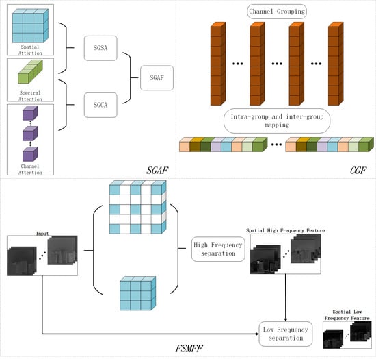
The spectrum-guided spatial/channel attention (SGSA/SGCA) module use spectral high-frequency information to optimize channel attention and spatial attention, so that it can be applied in spectral dimension. The proposed attention module can simultaneously focus on the spatial, spectral, and channel features of HSI.

(2)

A cross-fusion module for joint spectral features (CFJSF) combines features from three branches and fuses them through multi-head self-attention, sharing the attention map with other branches. This module allows the network to learn the differences between response curves of different features in the spectrum dimension.

(3)

The high- and low-frequency separated multi-level feature fusion (FSMFF) is designed for merging the multi-level features of HSIs. This module enhances the expression ability of the proposed network.

(4)

Channel grouping and fusion (CGF) uses channel grouping to enable feature information in one group to guide the mapping and transformation of another group of feature information. Each group of features only affects the adjacent group of features, which allows the network to refine the extracted fusion feature information and transmit it to the final upsampling operation.

2. Proposed Method

In this section, to introduce the proposed network, details on SCSFINet are presented in four parts: the overall framework, spectrum-guided attention fusion (SGAF) module, the high–low-frequency separated multi-level feature fusion (FSMFF) module, and the channel grouping and fusion (CGF) module. The goal of SCSFINet was to learn the mapping relationship between low-resolution (LR) and high-resolution (HR) HSIs with a size of $\mathrm{s}\times \mathrm{h}\times \mathrm{w}$ and $\mathrm{s}\times \mathrm{rh}\times \mathrm{rw}$, respectively; $\mathrm{s},\mathrm{h},\mathrm{w}$ and $\mathrm{r}$ represent the spectrum number, height, width, and up-scale factor of HSIs, respectively.

The super-resolution of HSIs was evaluated as follows:

$$I_{SR}=H\left(I_{LR};\theta \right)$$

(1)

where $I_{SR}$ and $I_{LR}$ represent the SR image and LR image, $\theta$ denotes the parameters of the proposed network, and $H(\cdot )$ indicates the mapping function of the SR method.

2.1. Overall Framework

The structure of the proposed network SCSFINet is shown in Figure 1. It has three parts, including shallow feature extraction, a spectral and spatial feature extraction (SSFE) module, and an image reconstruction module. In the first part, a 3 × 3 × 3 convolution filter was applied to extract the shallow feature $F_0$ of the input LR image $I_{LR}$. The value of $F_0$ was determined using the following Equation (2):

$$F_0=H_{333}\left(I_{LR}\right)$$

(2)

where $H_{333}(\cdot )$ indicates the convolution operation of size $3\times 3\times 3$.

Then, the shallow feature $F_0$ was sent to the designed spectral and spatial feature extraction (SSFE) module, which extracted the spectral–spatial joint feature using feature interweaving and fusion. The output of SSFE was obtained using Equation (3), as follows:

$$F_N=H_{SSFE}\left(F_0\right)$$

(3)

The spectral reflection curves corresponding to pixel points at different positions in the hyperspectral image were different (as shown in Figure 2). To help the proposed network adapt to the problem of different spectral reflection curves, the SSFE module first applied $n$ repeatedly cascaded spectrum-guided attention fusion (SGAF) modules to produce the joint characteristics of deep spectral, space, and channel. The output $F_n$ of the n-th SGAF was described as follows:

$$\begin{array}{l}{F}_n=H_{SGAF,n}\left(F_{n-1}\right)\\ \hspace{1em}\hspace{0.17em}=H_{SGAF,n}\left(H_{SGAF,n-1}\left(\cdots \left(H_{SGAF,1}\left(F_0\right)\right)\cdots \right)\right)\end{array}$$

(4)

where $H_{SGAF,n}$ indicates the operations of the n-th SGAF, which can be a composite function formed by three designed modules: SGSA, SGCA, and CFJSF. More details are presented below.

As more SGAFs were cascaded, the spatial expression ability of the network decreased while the semantic expression ability increased [28]. We built the high–low-frequency separated multi-level feature fusion (FSMFF) module to merge feature information from different stages. Based on the input features $F_1$, $F_2$, and $F_3$, which are produced by the first SGAF to the (n − 1)th SGAF, the feature after fusion $F_{FSMFF}$ was expressed as follows:

$$F_{FSMFF}=H_{FSMFF}\left(F_1;\dots ;F_{n-1}\right)$$

(5)

where $H_{FSMFF}(\cdot )$ indicates the feature fusion function.

At the end of the SSFE, we summed $F_n$, $F_{FSMFF}$, and the feature $F_0$ from the shallow feature extraction module to obtain the final feature $F_N$. The mathematical process can be described by Equation (6), as follows:

$$\begin{array}{l}{F}_N=H_{SSFE}\left(F_0\right)\\ \hspace{1em} =F_n+F_{FSMFF}+F_0\end{array}$$

(6)

In the reconstruction module, we applied the channel grouping and fusion (CGF) module for re-integrating the feature from SSFE and $1\times 1\times 1$ filters for adjusting the number of channels in order to restore the hyperspectral SR image. Based on the input $F_N$, the above process was expressed as follows:

$${\mathrm{I}}_{SR}=H_{up}\left(H_{111}\left(H_{CGF}\left(F_N\right)\right)\right)$$

(7)

where $H_{CGF}(\cdot )$ indicates the CGF module and $H_{up}(\cdot )$ indicates the upsampling function, which can vary with the scale factor.

In the learning-based SR field, the common upsampling operation requires using deconvolution [29] or sub-pixel convolution [30]. However, the “uneven overlap” of deconvolution [31] resulted in the formation of checkerboard artifacts in the output image. We applied sub-pixel convolution to reconstruct the SR image from the LR image.

2.2. Spectral and Spatial Feature Extraction Module (SSFE)

To integrate spectral features with spatial features and generate spectral attention features, this paper adopts the concept of residual skip connections from RCAN [16] to construct a network. The residual skip connections from RCAN enable low-frequency information to be transmitted through the network more quickly, while ensuring sufficient network depth to recover high-frequency information. The main body of the network uses the residuals of jump connections to learn nonlinear mapping, which contains several SGAFs.

(1) Spectrum-guided attention fusion (SGAF): It is well known that CBAM [32] and BAM [33] combine spatial attention and channel attention from series and parallel perspectives, respectively, to form more effective integrated attention. SGAF combines SGSA and SGCA in the way of hierarchical connection and cross-fusion. As shown in Figure 3, to obtain the joint feature from spectra, space, and channel and to integrate the spectral feature into spatial and channel dimensions, we constructed three parallel branches, each of which used features from different dimensions and exchanged features with other branches.

In the upper/lower branch, SGSA and SGCA are fused in a hierarchical connection. The above process was as follows:

$$F_{middle}^{n-1}={\mathrm{H}}_{333}\left(F_{n-1}\right)$$

(8)

$${\mathrm{F}}_{upper}=H_{SGSA-b}\left(H_{SGCA-a}\left(F_{middle}^{n-1}\right)\right)$$

(9)

$${\mathrm{F}}_{lower}=H_{SGCA-b}\left(H_{SGSA-a}\left(F_{middle}^{n-1}\right)\right)$$

(10)

where $H_{SGSA-a/b}(\cdot )$ indicates the SGSA-a/b module, and $H_{SGCA-a/b}(\cdot )$ indicates the SGCA-a/b module.

In the middle branch, the different features of the upper and lower branches will be transmitted in the CFJSF by way of cross-fusion. Due to the different response curves of the same target on the spectral axis, the middle branch combined its feature with two features from other branches (SGSA-a and SGCA-a), using the cross-fusion module for joint spectral features (CFJSF) to determine the correlation among the spectral dimensions. Equations (11)–(13) are as follows:

$$F_{SGCA-a}=H_{SGCA-a}\left(F_{middle}^{n-1}\right)$$

(11)

$$F_{SGSA-a}=H_{SGSA-a}\left(F_{middle}^{n-1}\right)$$

(12)

$$F_{CFJSF},F_{SAM}=H_{CFJSF}\left(F_{middle}^{n-1},F_{SGCA-a},F_{SGSA-a}\right)$$

(13)

where $H_{CFJSF}(\cdot )$ indicates the CFJSF module.

Furthermore, the adjusted feature was sent to the concatenation operation, and the self-attention probability map was sent to the second stage of the other two branches (SGSA-b and SGCA-b) for further modifying their features, as follows:

$$F_n=H_{111}\left([{\mathrm{F}}_{upper};F_{CFJSF};{\mathrm{F}}_{lower}\right])$$

(14)

where $[\cdot ]$ indicates the concatenation operation.

Compared with CBAM’s serial connection and BAM’s parallel connection, this module can improve the network’s feature emphasis on features from different domains in the feature map, as it combines SGSA (spectrum-guided spatial attention) and SGCA (spectrum-guided channel attention) using hierarchical fusion and cross-fusion.

(2) Spectrum-guided spatial attention (SGSA) and spectrum-guided channel attention (SGCA): SGSA and SGCA are shown in Figure 4. Compared to conventional spatial attention/channel attention, SGSA and SGCA applied HFGSA(high-frequency-guided spectrum adaptive) modules specifically designed to deal with spectral attention and avoided the unreasonable utilization of spectral information caused by the direct average processing of the spectral dimension to extend SA and CA directly into the spectral dimension.

There are two versions of SGSA (SGSA-a and SGSA-b) and SGCA (SGCA-a and SGCA-b). The versions with b received a self-attention probability map from CFJSF as the input to adjust the feature map.

Taking SGSA-a as an example, SGSA, like conventional SA, used average-pooling and max-pooling to determine the mean and maximum values of the input feature on the HW plane. For the spectral dimension, SGSA-a used HFGSA to obtain the spectral attention, which acted as the weight coefficient of spectral dimension, and then it was summed along the spectral dimension to obtain the feature map after adaptive adjustment. Equation (15) is as follows:

$$F_{SGSA-a}^1=Av{g}_S\left(H_{HFGSA}\left(F_{n-1})\right)\right)$$

(15)

where $H_{HFGSA}(\cdot )$ indicates the HFGSA module and $Av{g}_S(\cdot )$ indicates the average operation on the spectral dimension.

Note that in SGSA-b, the formula is changed to the following:

$$F_{SGSA-b}^1=Av{g}_S\left(H_{HFGSA}\otimes F_{SAM}\right)$$

(16)

where $F_{SAM}$ indicates the self-attention probability map and $\otimes$ indicates the matrix multiplication operation.

Then, conventional SA was applied to obtain the final feature, as follows:

$$F_{SGSA-a}^{max}={\max }_s\left(F_{SGSA-a}^1\right)$$

(17)

$$F_{SGSA-a}^{mean}={\mathrm{mean}}_s\left(F_{SGSA-a}^1\right)$$

(18)

$$F_{SGSA-a}^{out}=F_{n-1}\odot \sigma (H_{111}(F_{SGSA-a}^{max};F_{SGSA-a}^{mean}))$$

(19)

where $s$ indicates that the operation was performed in the spectral dimension.

The process for SGCA was quite different from that of SGSA. The SGCA-a first used a 2D convolution kernel to extract the spatial feature of the input feature, as follows:

$$F_{SGCA-a}^1=H_{133}\left(H_{333}\left(F_{n-1}\right)\right)$$

(20)

Unlike the $max$ and $mean$ operations in SGSA, as shown in Equations (17) and (18), respectively, these two operations in SGCA were used in the spatial dimension of the feature map, as follows:

$$F_{SGCA-a}^{max}={\max }_{HW}\left(F_{SGCA-a}^1\right)$$

(21)

$$F_{SGCA-a}^{mean}={\mathrm{mean}}_{HW}\left(F_{SGCA-a}^1\right)$$

(22)

$$F_{SGCA-a}^2={\mathrm{H}}_{111}\left(F_{SGCA-a}^{max};F_{SGCA-a}^{mean}\right)$$

(23)

where $HW$ indicates that the operation is performed in the spatial dimension.

Then, HFGSA was used to extract the correlation information of the input features along the spectral dimensions, as follows:

$$F_{SGCA-a}^3={\mathrm{Avg}}_s({\mathrm{H}}_{HFGSA}\left(F_{SGCA-a}^2\right))$$

(24)

The difference between SGCA-b and SGCA-a is shown in the following Equation (25), and the rest are the same:

$$F_{SGCA-a}^3={\mathrm{Avg}}_s({\mathrm{H}}_{HFGSA}\left(F_{SGCA-a}^2\otimes F_{SAM}\right))$$

(25)

Finally, SGCA-a used the compression and expansion method on the channel dimension to extract the relevant information of the input feature map in the channel dimension and then multiplied it with the input of $F_{n-1}$, as follows:

$$F_{SGCA-a}^{out}=\sigma \left(H_{111}\left(H_{111}\left(H_{HFGSA}\left(F_{SGCA-a}^3\right)\right)\right)\right)$$

(26)

Compared with CA and SA, this module not only focuses on the feature correlation information of spatial and channel domain, but also emphasizes the spectral dimension correlation features. Meanwhile, since the features of the spectral domain are fully extracted, the spectral information loss caused by the direct use of CA and SA for max-pooling and average-pooling of spectral dimensions can be avoided.

(3) High-frequency-guided spectrum adaptive mechanism (HFGSA): As shown in Figure 5d, it is believed that using the convolution kernel of a large receptive field in the spectral dimension can increase the detail information from spectral bands, while spectral high-frequency information can be obtained by using the difference in the feature map of the large and small receptive fields. The HFGSA consists of two main modules, spectral-FSM and spectral-HFA, as shown in Figure 5a. Spectral-FSM is applied to separate spectral high-frequency features, while spectral-HFA uses spectral high-frequency information to generate attention features.

Specifically, as shown in Figure 5c, spectral-FSM mainly uses two kinds of $3\times 1\times 1$ convolution kernels with different receptive fields (with/without dilation) for extracting the input features in the spectral dimension. Given that the input $F_{HFGSA}^{input}\in R^{C\times S\times H\times W}$, the feature was sent to two different convolution layers in parallel to generate spectral high-frequency features. $F_{SHF}$ was determined using Equations (27)–(29) as follows:

$$F_{SRF}=H_{311}^{wo}\left(H_{311}\left(F_{HFGSA}^{input}\right)\right)$$

(27)

$$F_{LRF}=H_{311}^w\left(H_{311}\left(F_{HFGSA}^{input}\right)\right)$$

(28)

$$F_{SHF}=F_{LRF}-F_{SRF}$$

(29)

where $C,S,H,andW$ indicate the number of channels, spectrum, height, and width, respectively, $H_{311}^w(\cdot )$ and $H_{311}^{wo}(\cdot )$ indicate the convolution layer of size $3\times 1\times 1$ with and without dilation, respectively, $F_{SRF}$ and $F_{LRF}$ indicate the small and large receptive field features, respectively, and $F_{SHF}$ is the high-frequency feature.

Spectral-HFA uses the high-frequency feature to generate the attention map for adjusting the small/large receptive field feature information, as shown in Figure 5b. Equations (30) and (31) are as follows:

$$F_{Spectral-HFA}^{SRF}=H_{311}^{wo}\left(F_{SRF}+F_{SRF}\odot \sigma \left(H_{311}^{wo}\left(F_{SHF}\right)\right)\right)$$

(30)

$$F_{Spectral-HFA}^{LRF}=H_{311}^w\left(F_{LRF}+F_{LRF}\odot \sigma \left(H_{311}^w\left(F_{SHF}\right)\right)\right)$$

(31)

where $F_{Spectral-HFA}^{SRF}$ and $F_{Spectral-HFA}^{LRF}$ indicate the output feature of the small/large receptive field from spectral-HFA, $\odot$ indicates the element-wise multiplication, and $\sigma$ indicates the sigmoid function.

Finally, the outputs of the two different receptive field spectral-HFAs were added and fused, and then the merged feature was sent to the sigmoid function layer to obtain the final spectral attention map. The final output of the module was obtained by multiplying the map and the original input, as follows:

$$out=F_{HFGSA}^{input}\odot \sigma \left(F_{Spectral-HFA}^{SRF}+F_{Spectral-HFA}^{LRF}\right)$$

(32)

The above method was used to design an adaptive attention mechanism for the spectral dimension, which solved the problem related to the effect of directly pooling the spectral dimension when applying HSIs to SA and CA.

(4) Cross-fusion module for joint spectral features (CFJSF): Although HFGSA adds an attention mechanism to the spectral dimension from the perspective of spectral high-frequency information, the $3\times 1\times 1$ convolution kernel is still sliding on the spectral dimension, its essence is still only able to obtain the correlation between k adjacent bands, and it cannot effectively obtain the context information of the entire spectral dimension.

Therefore, a self-attention mechanism will be used in this paper to make up for the deficiency of HFGSA in spectral context information extraction. However, due to the different spectral curves corresponding to different pixel points, a single self-attention mechanism will not be able to use the spectral curves of numerous ground objects in hyperspectral images, and too much self-attention will waste computing resources. In this paper, we will use the method of multiple self-attention mechanisms to extract the long-range correlation of the spectral dimension. Different from sequences, HSIs have a large number of effective features both in the space and spectral domain, so it is necessary to reasonably distinguish the key, query, and value to capture the spectral dimension correlation of hyperspectral images to the maximum extent.

In SGAF, the upper and lower branches are composed of SGSA and SGCA in series, while CFJSF connects SGSA-a and SGCA-a in parallel and sends them to CFJSF together with the middle branch. Since the self-attention probability matrix graph jointly generated by the key and query is used to guide the attention adjustment of value, the selection of the key and query should be the part that best reflects the features of HSI, namely SGSA-a and SGCA-a, because they represent the spectrum–space joint feature and spectrum-channel joint feature of HSI, respectively.

As shown in Figure 6, we used the multi-head self-attention mechanism to determine the correlation between spectra. There were three inputs in CFJSF, namely $F_{\mathrm{CFJSF}}^{in-1}$, $F_{\mathrm{CFJSF}}^{in-2}$ and $F_{\mathrm{CFJSF}}^{in-3}$, as in the following Equations (32)–(34):

$$F_{\mathrm{CFJSF}}^{in-1}=F_{middle}^{n-1}$$

(33)

$$F_{\mathrm{CFJSF}}^{in-2}=F_{middle}^{n-1}+F_{SGCA-a}$$

(34)

$$F_{\mathrm{CFJSF}}^{in-3}=F_{middle}^{n-1}+F_{SGSA-a}$$

(35)

First, the feature maps after $F_{\mathrm{CFJSF}}^{in-2}$ and $F_{\mathrm{CFJSF}}^{in-3}$ were concatenated and taken as the $\mathrm{Query}$ and $\mathrm{Key}$ of self-attention, and $F_{\mathrm{CFJSF}}^{in-1}$ was taken as the $\mathrm{value}$ of self-attention, as follows:

$$F_{QK}=H_{111}\left(\left[F_{\mathrm{CFJSF}}^{in-2};F_{\mathrm{CFJSF}}^{in-3}\right]\right)$$

(36)

$$F_V=F_{\mathrm{CFJSF}}^{in-1}$$

(37)

Then, these features were sent to $\mathrm{m}$ self-attention modules to generate eight self-attention probability maps and n adjusted features, as follows:

$$\begin{array}{c}{F}_{SAM,1},F_{\mathrm{CFJSF},1}=H_{self-att,1}\left(F_{QK},F_V\right)\\ F_{SAM,2},F_{\mathrm{CFJSF},2}=H_{self-att,2}\left(F_{QK},F_V\right)\\ \begin{array}{c}\cdot \\ \cdot \\ \cdot \end{array}\\ F_{SAM,m},F_{\mathrm{CFJSF},m}=H_{self-att,n}\left(F_{QK},F_V\right)\end{array}$$

(38)

where $H_{self-att,i}\left(i=1,2,\dots ,m\right)$ indicates the i-th self-attention function, and $F_{SAM,i},F_{\mathrm{CFJSF},i}\left(i=1,2,\dots ,m\right)$ indicates the i-th probability map and adjusted feature.

Finally, these probability maps were concatenated, and the merged map was sent to HFGSA-b in the next SGCA and SGSA in other branches. These adjusted features were concatenated into one, and the feature was sent to the final concatenation at the end of SGAF, as follows:

$$F_{SAM}=H_{133}\left(F_{SAM,1};F_{SAM,2};\dots ;F_{SAM,m}\right)$$

(39)

$$F_{\mathrm{CFJSF}}=H_{333}\left(F_{\mathrm{CFJSF},1};F_{\mathrm{CFJSF},2};\dots ;F_{\mathrm{CFJSF},m}\right)$$

(40)

$$F_{SGAF}=H_{333}\left(F_{SGSA}^2;F_{SGAF};F_{SGCA}^2\right)$$

(41)

where $F_{SGSA}^2$ and $F_{SGCA}^2$ indicate the second module after SGCA and SGSA in each branch, respectively. $F_{SAM}$ was sent to HFGSA-b for further feature extraction.

2.3. High–Low Frequency Separated Multi-Level Feature Fusion (FSMFF)

Densely connected networks, such as DenseNet [34] and SRDenseNet [35], and output features from different stages were merged by simple addition or concatenation. However, this simple fusion method using a point-by-point convolution kernel is only a weighted summation of features from different stages according to channel dimensions, which fails to make full use of information from feature space, such as spatial high-frequency information. As shown in Figure 7, to more effectively integrate the output feature from different stages and assist the reconstruction module to complete the SR image, we constructed the high–low-frequency separated multi-level feature fusion (FSMFF) module, inspired by octave convolution [36], based on a spatial frequency separation module (spatial-FSM), spatial high/low frequency feature mapping (spatial-HFFM/spatial-LFFM), and spatial high–low frequency exchange (spatial-HLFE).

There were $n-1$ features $F_{SGAF,1}$, …, $F_{SGAF,n-1}\in R^{C\times S\times H\times W}$ as inputs of FSMFF, which were from each stage of the network. First, we used 3D convolution of size $1\times 1\times 1$ after concatenation to obtain the preliminary fusion feature $F_{FSMFF}^{input}\in R^{C/q\times S\times H\times W}$, as follows:

$$F_{FSMFF}^{input}=H_{111}\left(F_{SGAF,1};\dots ;F_{SGAF,n-1}\right)$$

(42)

where $q$ indicates the channel downsampling factor to make an effective fusion of channel information.

Next, we obtained two different frequency features via spatial-FSM. Different from octave convolution, we use the spatial-FSM to artificially divide the high and low frequency features from the input feature, as shown in Figure 8. Spatial-FSM generates $F_{Spatial-H}\in R^{C/q\times S\times H\times W}$ by the difference in the different receptive field convolution layers in spatial dimensions. The $F_{Spatial-L}\in R^{C/q\times S\times H\times W}$ is obtained by subtracting the $F_{FSMFF}^{input}$ with $F_{Spatial-H}$, and the above process is as follows:

$$F_{Spatial-H}=H_{311}^w\left(H_{311}\left(F_{FSMFF}^{input}\right)\right)-H_{311}^{wo}\left(H_{311}\left(F_{FSMFF}^{input}\right)\right)$$

(43)

$$F_{Spatial-L}=TID(F_{FSMFF}^{input}-F_{Spatial-H})$$

(44)

where $TID(\cdot )$ means the trilinear interpolation downsampling operation.

After separating the spatial high and low frequency features, the high and low frequency features are, respectively, sent into the corresponding feature mapping module, as shown in Figure 9a.

$$F_{Spatial-H}^{\prime }=H_{333}\left(F_{Spatial-H}\right)$$

(45)

$$F_{Spatial-H}^{″}=H_{333}\left(F_{Spatial-H}^{\prime }+F_{Spatial-LH}\right)$$

(46)

$$F_{Spatial-L}^{\prime }=H_{333}\left(F_{Spatial-L}\right)$$

(47)

$$F_{Spatial-L}^{″}=H_{333}\left(F_{Spatial-L}^{\prime }+F_{Spatial-HL}\right)$$

(48)

Spatial-HFFM and spatial-LFFM ensure that the feature components of different spatial frequencies are carried out in different feature mapping branches. However, independent feature mapping is insufficient for multi-stage feature extraction, so it is also necessary to fuse feature components of different frequency features, as shown in Figure 9b. We performed spatial-HLFE to fuse the features from different spatial frequency, as follows:

$$F_{Spatial-HL}=TID\left(H_{333}\left(F_{Spatial-H}^{\prime }\right)\right)$$

(49)

$$F_{Spatial-LH}=TIU\left(H_{333}\left(F_{Spatial-L}^{\prime }\right)\right)$$

(50)

$$F_{FSMFF}^{fused}=F_{Spatial-H}^{″}+TIU\left(F_{Spatial-L}^{″}\right)$$

(51)

where $TIU(\cdot )$ means the trilinear interpolation upsampling operation.

The above operations combined the feature information from different stages to effectively use spatial high- and low-frequency information. After the fusion of high and low frequency information, we also applied the pixel self-attention mechanism after $F_{FSMFF}^{fused}$, which generated more detailed features for the final reconstruction stage.

Given that $F_{FSMFF}^{fused}\in R^{C_1\times S\times H\times W}$, where $C_1=C/q$, we applied channel-wise downsampling and upsampling of convolutional layers to further utilize the correlation between points. Then, a sigmoid activation function was used to normalize and generate the attention weight coefficients, which were applied to linearly weigh the features for obtaining the auxiliary feature. Finally, we used a pointwise convolution of size $1\times 1\times 1$ to restore the original number of channels.

$$F_{weight}=\sigma \left(H_{111}\left(H_{111}\left(F_{FSMFF}^{fused}\right)\right)\right)$$

(52)

$$F_{FSMFF}=H_{111}\left(F_{weight}\odot F_{FSMFF}^{fused}\right)$$

(53)

The FSMFF combined multi-level features by using high- and low-frequency separation and pixel-level self-attention mechanisms, thus, improving the nonlinear mapping and expression ability of the network effectively.

2.4. Channel Grouping and Fusion (CGF)

In the super-resolution reconstruction stage, the upsampling method based on subpixel convolution [30] is usually used directly. However, when the information in the LR space is limited, a well-designed module can compensate for the lack of important local information by distilling features in the HR space [37]. An efficient hyperfraction model can be considered as generating a relatively rough SR feature map, and then obtaining a more detailed SR feature map from the rough SR feature map through some fine operations.

We proposed the CGF to divide the feature map into several groups along the channel, as shown in Figure 10a. The rough SR feature map is transformed into a fine SR feature map by intra-group feature mapping and inter-group feature transfer. The k-th group was fused with the (k − 1)th group to obtain the new k-th group feature information. The (k − 1)th group generate the channel attention map to adjust the k-th group, as shown in Figure 10b. Then, the output features of each group were concatenated along the channel dimension and re-fused and adjusted through the convolution layer to obtain the pre-reconstructed feature. Finally, the channel of the pre-reconstructed feature was adjusted to $r^2$ times using point-wise convolution, and the result of the final super-resolution reconstruction was obtained using sub-pixel convolution, as follows:

$$\begin{array}{l}{F}_{\mathrm{CGF}}^0=F_N\\ \hspace{1em} \hspace{0.17em}\hspace{0.17em}=\left[F_{N,0},F_{N,1},\dots ,F_{N,\mathrm{k}}\right]\end{array}$$

(54)

$$F_{\mathrm{CGF},0}^0=F_{N,0}$$

(55)

$$\begin{array}{c}{F}_{\mathrm{CGF},1}^0=H_{333}\left(F_{N,1}+F_{N,0}\right)\odot CAM\left(F_{N,0}\right)\\ F_{\mathrm{CGF},2}^0=H_{333}\left(F_{N,2}+F_{N,1}\right)\odot CAM\left(F_{N,1}\right)\\ \begin{array}{c}\cdot \\ \cdot \\ \cdot \end{array}\\ F_{CGF,\mathrm{k}}^0=H_{333}\left(F_{N,\mathrm{k}}+F_{N,\mathrm{k}-1}\right)\odot CAM\left(F_{N,\mathrm{k}-1}\right)\end{array}$$

(56)

$$F_{CGF}^1=\left[F_{\mathrm{CGF},1}^0;F_{\mathrm{CGF},2}^0;\dots ;F_{CGF,\mathrm{k}}^0\right]$$

(57)

$$F_{CGF,1}^2=H_{333}\left(F_{CGF}^1\right)$$

(58)

$$I_{SR}=H_{up}\left(H_{111}\left(F_{CGF,1}^2\right)\right)$$

(59)

where $CAM(\cdot )$ indicates the channel attention layer.

Our proposed network was trained with the L1 norm as the loss function of the network, as follows:

$$\mathrm{Loss}\left(I_{SR},I_{HR}\right)=\frac{1}{N}{{\displaystyle \sum }}_{i=1}^N\left|I_{SR}^i-I_{HR}^i\right|$$

(60)

where $I_{SR}$ represents the reconstructed spectral image, $I_{HR}$ represents the original spectral image, and $N$ represents the number of training samples.

3. Experiments

In this section, we evaluated the proposed SCSFINet both quantitatively and qualitatively. First, we tested our SCSFINet on three common datasets and mentioned the specific implementation details. Then, we analyzed the performance of SCSFINet. Finally, we compared the proposed SCSFINet with Bicubic, VDSR, EDSR, MCNet, ERCSR, and MSFMNet.

3.1. Datasets

Among many hyperspectral datasets, we selected three of the most common datasets as the benchmark for verifying the proposed network performance in this study. These datasets were CAVE, Pavia Center, and Pavia University.

(1) CAVE: The CAVE dataset was collected by a cooled CCD camera that had a spectral width of 400–700 nm. This dataset had 512 pixels in both height and width and contained 32 hyperspectral images, each of which was divided into 31 spectral bands at a spectral interval of 10 nm. In the evaluation stage, we selected 7 images for testing and kept 25 images for training [23].

(2) Pavia Center (Pavia) and Pavia University (PaviaU): The Pavia Center (Pavia) dataset and Pavia University (PaviaU) dataset had a wavelength range of 430–860 nm, and they were collected using ROSIS sensors over the city of Pavia in northern Italy. Pavia had 102 spectral bands with 1096 pixels in height and 715 pixels in width, while PaviaU had 103 spectral bands. Both Pavia and PaviaU had nine categories of figures, but the categories of this dataset were not completely consistent. For more effective training and testing, starting from the upper left corner of these two datasets as the origin, we selected images with a size of $144\times 144$ as the test set and the other parts as the training set.

(3) Data preprocessing: Although the samples in the dataset belonged to the same distribution, there were differences in the distribution between the original samples without any processing. Thus, the input samples needed to be standardized via data preprocessing to improve the convergence speed of the network and the image reconstruction effect of the overall network [37]. We used the zero-mean standardization (Z-score) method to preprocess the dataset, which uses the mean and standard deviation of the dataset to adjust the data to the normal distribution. For HSIs, the average value and standard deviation of the pixels in each band were calculated, and the average vector and standard deviation vector along the spectral dimension were obtained, as follows:

$$x^{\prime }=\frac{x-\mu }{\sigma }$$

(61)

where $x,\mu$, $\sigma$, and $x^{\prime }$ indicate the original sample, the average value, the standard deviation of $x$ in each spectral band, and the standardized $x^{\prime }$, respectively.

After image reconstruction, the de-normalization operation was conducted through known $\mu$ and $\sigma$ to obtain the final $I_{SR}$.

3.2. Implementation Details

(1) Experiment settings: Since the number of spectra in different datasets was different, the setting of the number of spectra in the model was consistent with the input dataset. The number of feature channels (C) was set to 64. The number n in the SGAF module was set to 4, which implied that there were four repeatedly cascaded SGAFs to extract joint features of deep spectral, space, and channels. In the CFJSF module, eight self-attention modules were arranged in parallel. In the FSMFF module, the downsampling factor $q$ was set to $1/2$ to effectively fuse the channel information. In the CGF, the input feature was divided into four groups along the channel dimension, which was denoted as $k$.

The data preparation, network training, and the testing described in this study were conducted in MATLAB and Python environments. The hardware device consisted of four NVIDIA RTX2080Ti graphics cards.

In the settings of hyperparameters related to training, we selected the ADAM algorithm as the network optimizer to optimize and update the network parameters, which set the exponential decay rate of the biased first-order moment estimation and biased second-order moment estimation to 0.9 and 0.999, respectively, and the correction factor to 1 × 10⁻⁸. The initial learning rate of the network was set to 1 × 10⁻⁴, which decayed 0.1 times every 120 epochs for 400 epochs.

(2) Evaluation metrics: The super-resolution reconstruction task requires objective evaluation indicators to determine the effectiveness of the reconstruction algorithm. Therefore, we selected four evaluation methods for quantitatively evaluating the performance of the network reconstruction results, which included the peak signal-to-noise ratio (PSNR), mean peak signal-to-noise ratio (MPSNR), structural similarity (SSIM), and spectral angle mapping (SAM). They were defined as follows:

$$\mathrm{MSE}=\frac{1}{H\cdot W}{\displaystyle \sum }_{i=1}^H{\displaystyle \sum }_{j=1}^W{\left(X\left(i,j\right)-Y\left(i,j\right)\right)}^2$$

(62)

$$\mathrm{PSNR}=10\times {\log }_{10}\frac{{\left(2^{Bits}-1\right)}^2}{MSE}$$

(63)

$$\mathrm{MPSNR}=\frac{10}{B}{\displaystyle \sum }_{i=1}^B{\log }_{10}\frac{{\left(2^{Bits}-1\right)}^2}{MSE}$$

(64)

$$\mathrm{SSIM}=\frac{\left(2{\mu }_x{\mu }_y+C_1\right)\left(2{\sigma }_{xy}+C_2\right)}{\left({\mu }_x^2+{\mu }_y^2+C_1\right)\left({\sigma }_x^2+{\sigma }_y^2+C_2\right)}$$

(65)

$$\mathsf{\theta }\left(z^{\ast },z_h\right)={\cos }^{-1}\left(\frac{z_h^T{z}^{\ast }}{\sqrt[2]{{\left(z^{\ast }\right)}^T{z}^{\ast }}\sqrt[2]{z_h^T{z}_h}}\right)$$

(66)

$$\mathrm{SAM}=\frac{1}{H\cdot W}{\displaystyle \sum }_{i=1}^H{\displaystyle \sum }_{j=1}^W\theta \left(X\left(i,j\right),Y\left(i,j\right)\right)$$

(67)

where $\mathrm{MSE}(\cdot )$ denotes the mean square error function, $X$ and $Y$ denote the reconstructed HSI image $I_{SR}$ and the original ground-truth image $I_{HR}$, respectively, $i$ and $\mathrm{j}$ indicate the index of the image height $H$ and width $W$, respectively, $Bits$ indicates the image pixel depth, $B$ indicates the number of spectral bands of the HSI image, ${\mu }_x$ and ${\mu }_y$ indicate the mean value of $I_{SR}$ and $I_{HR}$, respectively, ${\sigma }_x$ and ${\sigma }_y$ denote the variance of $I_{SR}$ and $I_{HR}$, respectively, ${\sigma }_{xy}$ indicates the covariance between $I_{SR}$ and $I_{HR}$, $C_1$ and $C_2$ indicate the minima that prevent division by zero, $\mathsf{\theta }(\cdot )$ represents the spectral angle mapping function, $z^{\ast }$ and $z_h$ represent the pixel vector of $I_{SR}$ and $I_{HR}$, respectively, and $T$ represents the vector transpose operation.

3.3. Results and Analysis

To comprehensively demonstrate the advantages of the proposed network, we selected six popular methods for comparison, namely Bicubic, VDSR, EDSR, MCNet, MSFMNet, and ERCSR. The following were the subjective and objective test results obtained by using the method on the three datasets.

(1) CAVE dataset: As shown in Figure 11, to visualize the test images, we selected the 26th, 17th, and 9th spectral bands from the photo_and_face_ms as the RGB channels, which were generated by different methods at scale factor 8. We found that the result obtained by the Bicubic, VDSR, EDSR, MCNet, MSFMNet, and ERCSR methods differed considerably from the original high-resolution image in various aspects, especially the texture edge features. Specifically, due to the lack of proper use of spectral and spatial information in hyperspectral images, the result generated by the Bicubic, VDSR, and EDSR methods were particularly fuzzy, and the texture changed significantly. Although MCNet, MSFMNet, and ERCSR had specially designed basic modules for hyperspectral datasets, these modules used basic 2D/3D convolution to extract two-dimensional and three-dimensional features from hyperspectral datasets and did not use the connection between the whole spectral band and spatial information. Therefore, MCNet, MSFMNet, and ERCSR had certain distortions in some bright areas. To visually demonstrate the reconstruction effect of the proposed method using spectral dimension information, we determined the absolute pixel difference between the SR result of various methods and the original high-resolution image (Figure 11). Compared to these methods, because SCSFINet can fully utilize the correlation of the whole spectral band and the connection between the space and spectrum, SCSFINet performed well in the subjective vision of texture details, edge features, and facial parts.

The reflectance curves of the pixels randomly selected in different spectral bands in the results obtained using different methods are shown in Figure 12. The curve of SCSFINet was closer to the original high-resolution image curve.

To quantitatively evaluate the advantages of the method from multiple perspectives, the quantitative description of the four performance indicators in the CAVE dataset is presented in

Table 1. Quantitative evaluation of the data on hyperspectral image SR algorithms from the CAVE dataset for scale factors 2, 4, and 8. The numbers in bold indicate the best result and underlined numbers indicate the second best. ↑ indicates that the larger the value, the better the performance. ↓ indicates that the smaller the value, the better the performance.

Scale	Methods	PSNR ↑	MPSNR ↑	SSIM ↑	SAM ↓
	Bicubic	40.330	39.500	0.9820	3.311
	VDSR	44.456	43.531	0.9895	2.866
	EDSR	45.151	44.207	0.9907	2.606
×2	MCNet	45.878	44.913	0.9913	2.588
	ERCSR	45.972	45.038	0.9914	2.544
	MSFMNet	46.015	45.039	0.9917	2.497
	Ours	46.240	45.240	0.9921	2.474
	Bicubic	34.616	33.657	0.9388	4.784
	VDSR	37.027	36.045	0.9591	4.297
	EDSR	38.117	37.137	0.9626	4.132
×4	MCNet	38.589	37.679	0.9690	3.682
	ERCSR	38.626	37.738	0.9695	3.643
	MSFMNet	38.733	37.814	0.9697	3.676
	Ours	38.848	37.897	0.9699	3.630
	Bicubic	30.554	29.484	0.8657	6.431
	VDSR	32.184	31.210	0.8852	5.747
	EDSR	33.416	32.337	0.9002	5.409
×8	MCNet	33.607	32.520	0.9125	5.172
	ERCSR	33.624	32.556	0.9113	5.114
	MSFMNet	33.675	32.599	0.9136	5.084
	Ours	33.723	32.638	0.9134	5.027

, with the optimal results represented in bold font. Figure 13 displays a bar chart of the data corresponding to a scale factor of 2, as shown in Table 1. By observing the four quantitative indicators, we found that our method performed the best under the condition of upscale factors 2, 4, and 8. However, only the SSIM under upscale factor 8 was slightly lower than (but very close to) the optimal MSFMNet at 0.0002. To summarize, our method used the inter-spectral attention mechanism and the effective high-frequency and low-frequency feature fusion module to realize the feature correlation mapping between spectra and feature fusion at different stages, and fully extracted the spectral information from the hyperspectral images.

(2) Pavia Dataset: The subjective performance of different methods on the Pavia dataset for upscale factor 4 is shown in Figure 14. Among them, the 13th, 35th, and 64th spectral bands were used for the color generation of RGB channels. The obtained image of Bicubic was too fuzzy, and the details were blurred, while only the result of SCSFINet could more effectively reconstruct the details contained in the original image.

As shown in the absolute error image, ESRCR and MSFMNet only recovered part of the information on the street, which led to a large error between them and the original high-resolution image. The resulting graph of SCSFINet differed the least from the original image, which further confirmed that SCSFINet had excellent reliability in the reconstruction of complex structural information. From the perspective of spectral reconstruction, the reflectance curve of the pixels in the spectral range (Figure 15) indicated that the spectral curve of SCSFINet was closest to the original high-resolution image, which confirmed that the spectral reconstruction performance of SCSFINet was excellent even for the complex structure.

The quantitative description of the four performance indicators in the Pavia dataset with scale factors 2, 4, and 8 are shown in

Table 2. Quantitative evaluation of the data on hyperspectral image SR algorithms from the Pavia dataset for scale factors 2, 4, and 8. The numbers in bold indicate the best result and underlined numbers indicate the second best. ↑ indicates that the larger the value, the better the performance. ↓ indicates that the smaller the value, the better the performance.

Scale	Methods	PSNR ↑	MPSNR ↑	SSIM ↑	SAM ↓
	Bicubic	32.406	31.798	0.9036	4.370
	VDSR	35.392	34.879	0.9501	3.689
	EDSR	35.160	34.580	0.9452	3.898
×2	MCNet	35.124	34.626	0.9455	3.865
	ERCSR	35.602	35.099	0.9503	3.683
	MSFMNet	35.678	35.200	0.9506	3.656
	Ours	35.927	35.413	0.9540	3.627
	Bicubic	26.596	26.556	0.7091	7.553
	VDSR	28.328	28.317	0.7707	6.514
	EDSR	28.649	28.591	0.7782	6.573
×4	MCNet	28.791	28.756	0.7826	6.385
	ERCSR	28.862	28.815	0.7818	6.125
	MSFMNet	28.920	28.873	0.7863	6.300
	Ours	29.031	29.000	0.7943	5.873
	Bicubic	24.464	24.745	0.4899	7.648
	VDSR	24.526	24.804	0.4944	7.588
	EDSR	24.854	25.067	0.5282	7.507
×8	MCNet	24.877	25.096	0.5391	7.429
	ERCSR	24.965	25.190	0.5382	7.834
	MSFMNet	25.027	25.257	0.5464	7.449
	Ours	25.125	25.377	0.5553	7.404

. Figure 16 displays a bar chart of the data corresponding to a scale factor of 2, as shown in Table 2. The results of the experiment showed that the method was superior to other methods at different scales when analyzing the data in the Pavia dataset.

(3) PaviaU Dataset: The subjective performance of different methods on the PaviaU dataset for upscale factor 8 is shown in Figure 17. Among them, the 13th, 35th, and 64th spectral bands were used for the color generation of RGB channels. From the figure, it is evident that most of the methods, such as Bicubic and VDSR, produce reconstructed images that are generally blurry. EDSR’s reconstructions exhibit granulation and more noise. The reconstructed images of MCNet, ERCSR, and MSFMNet feature blurred roads in the lower right corner. In contrast, SCSFINet can effectively recover the details in the image.

The absolute error image also indicates that Bicubic and VDSR have large errors in recovering the street part, whereas EDSR, MCNet, ERCSR, and MSFMNet can only partially recover the street details. SCSFINet’s results show the least difference from the original image, demonstrating its reliability and superiority. Additionally, the reflectance curve of pixels in the spectral range, shown in Figure 18, confirms that SCSFINet has the closest spectral curve to the original high-resolution image. This indicates that SCSFINet’s spectral reconstruction performance is excellent, even for complex structures.

Table 3. Quantitative evaluation of the data on hyperspectral image SR algorithms from the PaviaU dataset for scale factors 2, 4, and 8. The numbers in bold indicate the best result and underlined numbers indicate the second best. ↑ indicates that the larger the value, the better the performance. ↓ indicates that the smaller the value, the better the performance.

Scale	Methods	PSNR ↑	MPSNR ↑	SSIM ↑	SAM ↓
	Bicubic	30.509	30.497	0.9255	3.816
	VDSR	33.988	34.038	0.9524	3.258
	EDSR	33.943	33.985	0.9511	3.334
×2	MCNet	33.695	33.743	0.9502	3.359
	ERCSR	33.857	33.910	0.9520	3.220
	MSFMNet	34.807	34.980	0.9582	3.460
	Ours	35.914	35.033	0.9584	3.068
	Bicubic	29.061	29.197	0.7322	5.248
	VDSR	29.761	29.904	0.7854	4.997
	EDSR	29.795	29.894	0.7791	5.074
×4	MCNet	29.889	29.993	0.7835	4.917
	ERCSR	30.049	30.164	0.7899	4.865
	MSFMNet	30.140	30.283	0.7948	4.861
	Ours	30.388	30.489	0.8068	4.692
	Bicubic	26.699	26.990	0.5936	7.179
	VDSR	26.737	27.028	0.5962	7.133
	EDSR	27.182	27.467	0.6302	6.678
×8	MCNet	27.201	27.483	0.6254	6.683
	ERCSR	27.288	27.548	0.6276	6.611
	MSFMNet	27.334	27.586	0.6356	6.615
	Ours	27.384	27.590	0.6427	6.576

presents the quantitative descriptions of the four performance indicators for scale factors 2, 4, and 8 in the PaviaU dataset. In addition, Figure 19 displays the data under scale factor 2 in Table 3. The experimental results clearly demonstrate the superiority of our proposed method over other existing methods in analyzing PaviaU datasets at different scales. Considering that both Pavia and PaviaU datasets were smaller than the CAVE dataset, we found that our method also performed well with small datasets.

3.4. Ablation Study

In this section, we evaluated the proposed network from three aspects, including the study of SGAF, FSMFF, and CGF. For comparing the modules, we determined the results for a scale factor of 2 using the CAVE dataset.

As shown in Figure 20, to better explain our method, we constructed a baseline model corresponding to SCSFINet, which removed the proposed HSGFA, CFJSF, FSMFF, and CGF modules. The baseline model only had standard channel attention and spatial attention in parallel and series.

The effects of the ablation research on CFJSF, HFGSA, FSMFF, and CCG are shown in

Table 4. Ablation study results on evaluating the efficency of the network structure on the CAVE dataset of scale factor 2.

	1	2	3	4	5
CFJSF	✗	✓	✓	✓	✓
HFGSA	✗	✗	✓	✓	✓
FSMFF	✗	✗	✗	✓	✓
CGF	✗	✗	✗	✗	✓
PSNR	45.516	45.744	45.998	46.150	46.240
mPSNR	44.574	44.776	44.983	45.144	45.240
SSIM	0.9911	0.9914	0.9917	0.9919	0.9921
SAM	2.602	2.573	2.521	2.491	2.474

and Figure 21. To compare the impact of different components on the network without any bias, we used five collocation methods to conduct ablation surveys.

The results of the ablation study presented in Table 4 showed that when the network lacked any of the proposed modules, the performance was the worst. Because the baseline was equivalent to ignoring the spectral dimension of hyperspectral images and different features from different stages, it prevented the network from fully utilizing the spectral information and spatial information for learning. When the baseline model added the spectral dimension learning modules CFJSF and HFGSA, the performance indicators of the network improved significantly, which showed that the two modules designed in this study helped the spectral dimension of the network in learning. They enabled the network to learn spectral features along the spectral dimension, and they also fully integrated the features with the spatial features. When FSMFF and CCG were added to the baseline, the performance of the network improved significantly by 0.157 dB and 0.09 dB, respectively. Compared to the baseline, each experiment presented in Table 3 produced better results for the performance indicators. The results showed that each module was an indispensable link for the network.

4. Conclusions

In this study, we proposed a method for hyperspectral super-resolution which had good performance and generalization abilities for multiple datasets. SCSFINet designed several efficient modules to better learn the spectral and spatial joint characteristics of HSI. In order to extract more features from the spectrum, a HFGSA module is designed, which can effectively learn spectral features by combining spectral high-frequency information with an attention mechanism. The CFJSF module extracts the long-range correlation of the spectral dimension from the perspective of spectral context, so as to make up for the shortcoming that HFGSA can only use the features between several adjacent bands. Meanwhile, SGAF combined with SGSA, SGCA, and CFJSF effectively fused the features of spectral domain, spatial domain, and channel domain from the perspective of hierarchical fusion and cross-fusion. In addition, a FSMFF module is designed, and features of different frequency components are extracted and finally fused by means of spatial high- and low-frequency separation, so as to achieve efficient multi-level feature fusion. The designed CGF carries out feature interaction between groups in the form of channel grouping to help the network generate more detailed feature maps.

Based on the results of the experiment using several datasets, we showed that the effectiveness and generalization of SCSFINet were satisfactory, and the subjective and objective experimental results obtained using our method were better than those obtained using other methods.

References

1. Jalal, R.; Iqbal, Z.; Henry, M.; Franceschini, G.; Islam, M.S.; Akhter, M.; Khan, Z.T.; Hadi, M.A.; Hossain, M.A.; Mahboob, M.G.; et al. Toward Efficient Land Cover Mapping: An Overview of the National Land Representation System and Land Cover Map 2015 of Bangladesh. IEEE J. Sel. Top. Appl. Earth Obs. Remote Sens. 2019, 12, 3852–3861. [Google Scholar] [CrossRef]
2. Zhong, P.; Wang, N.; Zheng, Z.; Xia, J. Monitoring of drought change in the middle reach of Yangtze River. In Proceedings of the International Geoscience and Remote Sensing Symposium (IGARSS), Valencia, Spain, 22–27 July 2018; Volume 2018, pp. 4935–4938. [Google Scholar]
3. Goetzke, R.; Braun, M.; Thamm, H.-P.; Menz, G. Monitoring and modeling urban land-use change with multitemporal satellite data. In Proceedings of the International Geoscience and Remote Sensing Symposium (IGARSS), Boston, MA, USA, 8–11 July 2008; Volume 4, pp. 510–513. [Google Scholar]
4. Darweesh, M.; Al Mansoori, S.; AlAhmad, H. Simple Roads Extraction Algorithm Based on Edge Detection Using Satellite Images. In Proceedings of the 2019 IEEE 4th International Conference on Image, Vision and Computing, ICIVC 2019, Xiamen, China, 5–7 July 2019; pp. 578–582. [Google Scholar]
5. Kussul, N.; Shelestov, A.; Yailymova, H.; Yailymov, B.; Lavreniuk, M.; Ilyashenko, M. Satellite Agricultural Monitoring in Ukraine at Country Level: World Bank Project. In Proceedings of the International Geoscience and Remote Sensing Symposium (IGARSS), Waikoloa, HA, USA, 26 September–2 October 2020; pp. 1050–1053. [Google Scholar]
6. Di, Y.; Xu, X.; Zhang, G. Research on secondary analysis method of synchronous satellite monitoring data of power grid wildfire. In Proceedings of the 2020 IEEE International Conference on Information Technology, Big Data and Artificial Intelligence, ICIBA 2020, Chongqing, China, 6–8 November 2020; pp. 706–710. [Google Scholar]
7. Keys, R. Cubic convolution interpolation for digital image processing. IEEE Trans. Acoust. Speech Signal Process. 1981, 29, 1153–1160. [Google Scholar] [CrossRef]
8. Hou, H.; Andrews, H. Cubic splines for image interpolation and digital filtering. IEEE Trans. Acoust. Speech Signal Process. 1987, 26, 508–517. [Google Scholar]
9. Stark, H.; Oskoui, P. High-resolution image recovery from image-planear rays, using convex projection. J. Opt. Soc. Am. 1989, 6, 1715–1726. [Google Scholar] [CrossRef] [PubMed]
10. Irani, M.; Peleg, S. Improving resolution by image registration. CVGIP: Graphcial Model. Image Process. 1991, 53, 231–239. [Google Scholar] [CrossRef]
11. Schultz, R.R.; Stevenson, R.L. Extraction of high-resolution frames from video sequences. IEEE Trans. Image Process. 1996, 5, 996–1011. [Google Scholar] [CrossRef] [PubMed]
12. Dong, C.; Loy, C.C.; He, K.; Tang, X. Image super-resolution using deep convolutional networks. IEEE Trans. Pattern Anal. Mach. Intell. 2015, 38, 295–307. [Google Scholar] [CrossRef] [PubMed]
13. Kim, J.; Lee, J.K.; Lee, K.M. Accurate image super-resolution using very deep convolutional networks. In Proceedings of the IEEE Computer Society Conference on Computer Vision and Pattern Recognition, Las Vegas, NV, USA, 26 June–1 July 2016; Volume 2016-December, pp. 1646–1654. [Google Scholar]
14. Lim, B.; Son, S.; Kim, H.; Nah, S.; Lee, K.M. Enhanced Deep Residual Networks for Single Image Super-Resolution. In Proceedings of the IEEE conference on computer vision and pattern recognition, Honolulu, HI, USA, 21–26 July 2017. [Google Scholar]
15. Ledig, C.; Theis, L.; Huszár, F.; Caballero, J.; Cunningham, A.; Acosta, A.; Aitken, A.; Tejani, A.; Totz, J.; Wang, Z.; et al. Photo-realistic single image super-resolution using a generative adversarial network. In Proceedings of the IEEE Conference on Computer Vision and Pattern Recognition, Honolulu, HI, USA, 21–26 July 2017; pp. 4681–4690. [Google Scholar]
16. Zhang, Y.; Li, K.; Li, K.; Wang, L.; Zhong, B.; Fu, Y. Image super-resolution using very deep residual channel attention networks. In Proceedings of the European Conference on Computer Vision (ECCV), Munich, Germany, 8–14 September 2018; pp. 286–301. [Google Scholar]
17. Mei, S.; Yuan, X.; Ji, J.; Wan, S.; Hou, J.; Du, Q. Hyperspectral image super-resolution via convolutional neural network. In Proceedings of the International Conference on Image Processing, ICIP, Athens, Greece, 7–10 October 2018; Volume 2017-September, pp. 4297–4301. [Google Scholar]
18. Yang, J.; Zhao, Y.-Q.; Chan, J.C.-W.; Xiao, L. A Multi-Scale Wavelet 3D-CNN for Hyperspectral Image Super-Resolution. Remote Sens. 2019, 11, 1557. [Google Scholar] [CrossRef]
19. Li, Q.; Wang, Q.; Li, X. Exploring the Relationship Between 2D/3D Convolution for Hyperspectral Image Super-Resolution. IEEE Trans. Geosci. Remote Sens. 2021, 59, 8693–8703. [Google Scholar] [CrossRef]
20. Li, J.; Cui, R.; Li, B.; Li, Y.; Mei, S.; Du, Q. Dual 1D-2D Spatial-Spectral CNN for Hyperspectral Image Super-Resolution. In Proceedings of the IGARSS 2019—2019 IEEE International Geoscience and Remote Sensing Symposium, Yokohama, Japan, 28 July–2 August 2019; pp. 3113–3116. [Google Scholar] [CrossRef]
21. Liu, D.; Li, J.; Yuan, Q. Enhanced 3D Convolution for Hyperspectral Image Super-Resolution. In Proceedings of the 2021 IEEE International Geoscience and Remote Sensing Symposium IGARSS, Brussels, Belgium, 11–16 July 2021; pp. 2452–2455. [Google Scholar] [CrossRef]
22. Li, Q.; Wang, Q.; Li, X. Mixed 2D/3D Convolutional Network for Hyperspectral Image Super-Resolution. Remote Sens. 2020, 12, 1660. [Google Scholar] [CrossRef]
23. Zhang, J.; Shao, M.; Wan, Z.; Li, Y. Multiscale Feature Mapping Network for Hyperspectral Image Super-Resolution. Remote Sens. 2021, 13, 4180. [Google Scholar] [CrossRef]
24. Hu, J.; Jia, X.; Li, Y.; He, G.; Zhao, M. Hyperspectral Image Super-Resolution via Intrafusion Network. IEEE Trans. Geosci. Remote Sens. 2020, 58, 7459–7471. [Google Scholar] [CrossRef]
25. Liu, D.; Li, J.; Yuan, Q. A Spectral Grouping and Attention-Driven Residual Dense Network for Hyperspectral Image Super-Resolution. IEEE Trans. Geosci. Remote Sens. 2021, 59, 7711–7725. [Google Scholar] [CrossRef]
26. Wang, X.; Ma, J.; Jiang, J. Hyperspectral Image Super-Resolution via Recurrent Feedback Embedding and Spatial–Spectral Consistency Regularization. IEEE Trans. Geosci. Remote Sens. 2022, 60, 1–13. [Google Scholar] [CrossRef]
27. Li, J.; Cui, R.; Li, B.; Song, R.; Li, Y.; Dai, Y.; Du, Q. Hyperspectral Image Super-Resolution by Band Attention Through Adversarial Learning. IEEE Trans. Geosci. Remote Sens. 2020, 58, 4304–4318. [Google Scholar] [CrossRef]
28. Yan, Y.; Xu, X.; Chen, W.; Peng, X. Lightweight Attended Multiscale Residual Network for Single Image Super-Resolution. IEEE Access 2021, 9, 52202–52212. [Google Scholar] [CrossRef]
29. Dong, C.; Loy, C.C.; Tang, X. Accelerating the super-resolution convolutional neural network. In Proceedings of the European Conference on Computer Vision, Amsterdam, The Netherlands, 11–14 October 2016; pp. 391–407. [Google Scholar]
30. Shi, W.; Caballero, J.; Huszár, F.; Totz, J. Real-Time Single Image and Video Super-Resolution Using an Efficient Sub-Pixel Convolutional Neural Network. In Proceedings of the IEEE Computer Society Conference on Computer Vision and Pattern Recognition, Las Vegas, NV, USA, 26 June–1 July 2016; Volume 2016-December, pp. 1874–1883. [Google Scholar]
31. Odena, A.; Dumoulin, V.; Olah, C. Deconvolution and Checkerboard Artifacts. Distill 2016. [Google Scholar] [CrossRef]
32. Woo, S.; Park, J.; Lee, J.-Y.; Kweon1, I.S. Cbam: Convolutional block attention module. In Proceedings of the European Conference on Computer Vision (ECCV), Munich, Germany, 8–14 September 2018. [Google Scholar]
33. Park, J.; Woo, S.; Lee, J.-Y.; Kweon, I.S. Bam: Bottleneck attention module. arXiv 2018, arXiv:1807.06514. [Google Scholar]
34. Huang, G.; Liu, Z.; Van Der Maaten, L.; Weinberger, K.Q. Densely connected convolutional networks. In Proceedings of the 30th IEEE Conference on Computer Vision and Pattern Recognition, CVPR 2017, Honolulu, HA, USA, 21–26 July 2017; Volume 2017-January, pp. 2261–2269. [Google Scholar]
35. Tong, T.; Li, G.; Liu, X.; Gao, Q. Image Super-Resolution Using Dense Skip Connections. In Proceedings of the IEEE International Conference on Computer Vision, Venice, Italy, 22–29 October 2017; Volume 2017-October, pp. 4809–4817. [Google Scholar]
36. Chen, Y.; Fan, H.; Xu, B.; Yan, Z.; Kalantidis, Y.; Rohrbach, M.; Shuicheng, Y.; Feng, J. Drop an Octave: Reducing Spatial Redundancy in Convolutional Neural Networks with Octave Convolution. In Proceedings of the 2019 IEEE/CVF International Conference on Computer Vision (ICCV), Seoul, Korea, 27 October–2 November 2019; pp. 3434–3443. [Google Scholar] [CrossRef]
37. Zhang, J.; Long, C.; Wang, Y.; Piao, H.; Mei, H.; Yang, X.; Yin, B. A Two-Stage Attentive Network for Single Image Super-Resolution. IEEE Trans. Circuits Syst. Video Technol. 2022, 32, 1020–1033. [Google Scholar] [CrossRef]
Figure 1. The overall architecture of the spectral correlation and spatial high–low frequency information of the hyperspectral image feature fusion network (SCSFINet).
Remotesensing 15 02472 g001
Figure 2. The reflection curve of seven points randomly selected in the photo_and_face_ms image from the CAVE dataset on spectral dimension. Seven points were randomly selected from the CAVE test image photo_and_face_ms, which has dimensions of 512 × 512. Each point’s coordinates (x, y) and dimensions (31) correspond to 31 spectral response values at that location.
Remotesensing 15 02472 g002
Figure 3. (a) CBAM. (b) BAM. (c) The architecture of the spectrum-guided attention fusion (SGAF); © represents the concatenation operation.
Remotesensing 15 02472 g003
Figure 4. (a,c) Architecture of the SGSA-a/b. (b,d) Architecture of the SGCA-a/b. Matrix multiplication only works if there is an input F S A M .
Remotesensing 15 02472 g004
Figure 5. (a) Architecture of the high-frequency-guided spectrum adaptive mechanism (HFGSA). (b) Architecture of the spectral high-frequency attention (spectral-HFA) module. (c) Architecture of the spectral frequency separation module (spectral-FSM). (d) Comparison of feature maps of different receptive fields. Due to the use of a larger receptive field convolution kernel along the spectral dimension, the detail information in the large spectral receptive field feature map is richer than the original input and small spectral receptive field feature map, so the obtained high-frequency information has more texture details than the original input.
Remotesensing 15 02472 g005
Figure 6. The architecture of the cross-fusion module for joint spectral features (CFJSF). © stands for the concatenation.
Remotesensing 15 02472 g006
Figure 7. The architecture of the high–low-frequency separated multi-level feature Fusion (FSMFF).
Remotesensing 15 02472 g007
Figure 8. The architecture of the spatial frequency separation module (spatial-FSM).
Remotesensing 15 02472 g008
Figure 9. (a) The architecture of the spatial high-frequency feature mapping (spatial-HFM) and spatial high-frequency feature mapping (spatial-LFM). (b) The architecture of the spatial high–low frequency exchange (spatial-HLFE).
Remotesensing 15 02472 g009
Figure 10. (a)The architecture of channel grouping and fusion (CGF). (b) The architecture for generating the channel attention map (CAM).
Remotesensing 15 02472 g010
Figure 11. Reconstruction results and absolute error map comparisons of various algorithms for the test image photo_and_face_ms. The reconstructed image of the spectral band 26-17-9 was used as the RGB channel with a scale factor of 8.
Remotesensing 15 02472 g011
Figure 12. A visual comparison of spectral distortion for the image photo_and_face_ms (170, 60), (280, 80), and (450, 300) from the CAVE dataset.
Remotesensing 15 02472 g012
Figure 13. Bar charts depicting the four evaluation indicators on the CAVE dataset of scale factor 2. (a) PSNR. (b) mPSNR. (c) SSIM. (d) SAM.
Remotesensing 15 02472 g013aRemotesensing 15 02472 g013b
Figure 14. The results of reconstruction and absolute error map comparisons of various algorithms using the Pavia Center dataset. The reconstructed image of spectral band 64-35-13 was used as the RGB channel with a scale factor of 4.
Remotesensing 15 02472 g014
Figure 15. A visual comparison of the spectral distortion of the images (80, 140), (120, 80), and (140, 15) from the Pavia Center dataset.
Remotesensing 15 02472 g015
Figure 16. Bar charts depicting the four evaluation indicators on the Pavia dataset of scale factor 2. (a) PSNR. (b) mPSNR. (c) SSIM. (d) SAM.
Remotesensing 15 02472 g016aRemotesensing 15 02472 g016b
Figure 17. The results of reconstruction and absolute error map comparisons of various algorithms using the PaviaU University dataset. The reconstructed image of spectral band 64-35-13 was used as the RGB channel with a scale factor of 8.
Remotesensing 15 02472 g017
Figure 18. A visual comparison of spectral distortion for the image (77, 39), (86, 91), and (132, 124) from the PaviaU dataset.
Remotesensing 15 02472 g018
Figure 19. Bar charts depicting the four evaluation indicators on the PaviaU dataset of scale factor 2. (a) PSNR. (b) mPSNR. (c) SSIM. (d) SAM.
Remotesensing 15 02472 g019aRemotesensing 15 02472 g019b
Figure 20. The architecture of the baseline network. Compared to SCSFINet, the baseline removed the designed SGAF, FSMFF, and CGF modules and only retained the basic structure.
Remotesensing 15 02472 g020
Figure 21. Bar charts depicting the four evaluation indicators of the ablation experiment. (a) PSNR. (b) mPSNR. (c) SSIM. (d) SAM.
Remotesensing 15 02472 g021aRemotesensing 15 02472 g021b