Construction and Assessment of a Drought-Monitoring Index Based on Multi-Source Data Using a Bias-Corrected Random Forest (BCRF) Model

Abstract

Agricultural drought significantly impacts agricultural production, highlighting the need for accurate monitoring. Accurate agricultural-drought-monitoring models are critical for timely warning and prevention. The random forest (RF) is a popular artificial intelligence method but has not been extensively studied for agricultural drought monitoring. Here, multi-source remote sensing data, including surface temperature, vegetation index, and soil moisture data, were used as independent variables; the 3-month standardized precipitation evapotranspiration index (SPEI_3) was used as the dependent variable. Soil texture and terrain data were used as auxiliary variables. The bias-corrected RF model was used to construct a random forest synthesized drought index (RFSDI). The drought-degree determination coefficients (R2) of the training and test sets reached 0.86 and 0.89, respectively. The RFSDI and SPEI_3 fit closely, with a correlation coefficient (R) above 0.92. The RFSDI accurately reflected typical drought years and effectively monitored agricultural drought in Northeast China (NEC). In the past 18 years, agricultural drought in NEC has generally decelerated. The degree and scope of drought impacts from 2003 to 2010 were greater than those from 2010 to 2020. Agricultural drought occurrence in NEC was associated with dominant climatic variables such as precipitation (PRE), surface temperature (Ts), relative humidity (RHU), and sunshine duration (SSD), alongside elevation and soil texture differences. The agricultural drought occurrence percentage at 50–500 m elevations reached 94.91%, and the percentage of occurrence in loam and sandy soils reached 90.31%. Water and temperature changes were significantly correlated with the occurrence of agricultural drought. Additionally, NEC showed an alternating cycle of drought and waterlogging of about 10 years. These results have significant application potential for agricultural drought monitoring and drought prevention in NEC and demonstrate a new approach to comprehensively evaluating agricultural drought.

1. Introduction

Against the backdrop of global warming, droughts are becoming increasingly frequent, lasting longer and affecting wider areas [1]. China, situated in Eastern Asia west of the Pacific Ocean, is persistently impacted by the Pacific monsoon climate, leading to periodic droughts [2]. Over the last two decades, more than 50% of China’s agricultural natural disaster losses have been caused by droughts [3]. In NEC, prolonged droughts have not only seriously impacted the ecological environment but also hindered the sustainable development of the agricultural economy [4]. Scholars have used traditional meteorological and remote sensing drought indices to monitor the spatial pattern and occurrence of droughts in NEC [5,6]. These studies have shown that the frequency and intensity of droughts are higher in southern NEC and lower in northern NEC, with the most drought-prone areas concentrated in the central plains. Spring droughts have the highest frequency and severity, while summer droughts are the weakest. The impact of spring droughts is stronger than the impacts of summer and autumn droughts.

Agricultural drought can be described as a soil moisture imbalance caused by long-term extreme weather that affects the normal growth of crops. Traditional agricultural-drought-monitoring methods mainly include field fixed-point monitoring and random investigation methods [7], which have the disadvantages of low efficiency, poor accuracy, and requiring extensive time and human labor. At present, it is difficult to meet the needs of real-time, large-scale agricultural drought monitoring. With the development of meteorological early-warning and remote sensing technologies, the problem of obtaining regional soil drought conditions in a timely and accurate manner has been effectively addressed. Currently, a wide range of different types of comprehensive surface information can be obtained from actual meteorological observation data recorded at meteorological observation stations and through satellite remote sensing. Thus, the use of meteorological and remote sensing technologies for monitoring and evaluating crop growth has become an important research topic in the fields of agrometeorology and agricultural remote sensing [8].

Currently, two primary methods are used for monitoring agricultural drought: meteorological monitoring based on meteorological data measured at specific sites and agricultural drought monitoring based on remote sensing data. The traditional meteorological drought method is relatively mature and provides accurate data, and it is thus widely used for meteorological agricultural drought monitoring in China [9]. Agricultural drought monitoring based on meteorological data typically involves the use of data observed at meteorological stations to calculate drought indices and monitor drought occurrence. Currently, widely used meteorological agricultural-drought-monitoring indicators include the standardized precipitation index (SPI) and the SPEI [10]. While meteorological data are highly accurate and readily available, the spatial distribution of meteorological stations is not uniform, making it challenging to monitor high-precision droughts in sparsely populated areas [11]. Furthermore, agricultural drought monitoring based on meteorological data does not consider the water demand state of vegetation or the water supply information of the soil, limiting its usefulness in agricultural drought monitoring. Remote sensing monitoring is widely used due to its advantages of high spatiotemporal resolution, continuous and easy access to data in both space and time, and ability to retrieve soil moisture, vegetation growth, and evapotranspiration information. These advantages compensate for the shortcomings of the insufficient agricultural-drought-monitoring accuracies obtained in areas with sparse meteorological stations. To improve the accuracy of agricultural drought monitoring, Liu et al. [12] have introduced remote sensing technology into agricultural-drought-monitoring studies based on the two drought carriers of vegetation and surface soil and established agricultural drought remote sensing monitoring indices from different perspectives.

Currently, remote sensing agricultural-drought-monitoring methods can mainly be divided into three categories. The first category is the vegetation index drought-monitoring model. The widely used indexes include the normalized difference vegetation index and vegetation condition index. The second category is the combined use of a vegetation index and land surface temperature, mainly including the vegetation health index and vegetation supply water index; the third category is drought-monitoring methods based on surface energy balance theory and active and passive microblog remote sensing.

Due to the complexity of the Earth–atmosphere system and the diversity of organisms, the monitoring accuracies of remote sensing indices may be affected by many factors, such as the considered time and space, crop type, soil information in the planting area, topographic factors, and different developmental stages of crops [13]. To improve the accuracy of agricultural drought monitoring, Kogan et al. and Hu et al. [14,15] have discussed the spatiotemporal applicability differences among existing remote sensing indices for agricultural drought monitoring. Guo et al. and Merino et al. [16,17] have optimized index construction parameters to revise existing remote sensing indices. Some scholars have also shown that elevation, precipitation, and temperature affect drought. Furthermore, remote sensing data have limitations; for example, they ignore the influence of elevation on temperature, thereby reducing the accuracies of temperature remote sensing products in high-elevation areas. To address this, Qutbudin et al. [18] have used elevation data to correct remote sensing data and combined the corrected data to perform agricultural drought monitoring.

The formation of agricultural drought is not dependent solely on the interactions among precipitation, temperature, and vegetation. Other factors, such as evaporation, topography, and soil information, are also important in the formation of agricultural drought [19]. Therefore, relying on a single factor such as precipitation or temperature is insufficient to accurately describe the occurrence of drought. Instead, a comprehensive approach that considers information from the atmosphere, vegetation, and soil is necessary to obtain accurate agricultural-drought-monitoring results. Several scholars have begun studying agricultural drought monitoring based on multi-source remote sensing data. Multiple linear regression [20], principal component analysis [21], and objective weighting [22] methods have been used to construct comprehensive drought indices. However, these methods of constructing a multi-factor agricultural-drought-monitoring model through linear combinations are unable to express the nonlinear relationships between different drought factors. To overcome this limitation, Qiong et al. [23] have started using machine learning models such as artificial neural networks and random forest models to construct agricultural-drought-monitoring models.

In addition, some scholars have tried to combine meteorological monitoring with remote sensing monitoring to comprehensively consider the factors that cause drought, such as soil moisture and meteorological precipitation [24]. Brown et al. [25] proposed the agricultural drought index by linearly adding the vegetation water supply index and the precipitation anomaly drought index with weights, and this method has shown good results in practical applications. Brown et al. developed the vegetation drought response index (VegDRI) by combining traditional meteorological agricultural-drought-monitoring indicators, remote sensing monitoring indicators, and other biophysical information. The VegDRI takes into account factors such as the vegetation growth status, precipitation surplus or deficit, and ecological environment parameters, including land cover types and topography, and has achieved good application results in agricultural drought monitoring in seven states in the north-central United States.

The above research was based on multi-source data and considered the factors that cause drought, providing a theoretical basis for this paper. However, the accuracy of such models depends on the response degrees of dependent variables to drought in the study area, and the adaptability of different dependent variables may vary among different study areas. Additionally, dependent variables may have many calculation parameters, making data acquisition difficult, which may limit their effectiveness [26]. Therefore, this paper attempts to establish a qualitative comprehensive agricultural-drought-monitoring model based on multi-source data using meteorological stations and remote sensing as data sources while comprehensively considering factors such as precipitation surplus or deficit, vegetation growth status, soil moisture, and topography.

In general, remote sensing monitoring of agricultural drought has a wide range of applications. In recent years, the northeast region has been affected by the East Asian tropical monsoon and the subtropical monsoon, and the abnormal atmospheric circulation has caused frequent drought in the spring maize growing season in the northeast. At the same time, due to the influence of specific geographical factors, the agricultural drought in Northeast China is complex and changeable, and it is difficult for the remote sensing index of a single data source to accurately identify agricultural drought. Therefore, it is necessary to comprehensively consider the interaction of soil, vegetation, atmosphere, and other factors to construct a new drought index to more accurately identify agricultural drought. To this end, this study aims to address the following aspects:

(1)

This study proposes a new index suitable for agricultural drought monitoring in the NEC region based on the bias-corrected random forest (BCRF) model using multi-source data.

(2)

The applicability of the new agricultural-drought-monitoring index in NEC is evaluated, and the new index is used to explore the spatiotemporal patterns of agricultural drought in NEC, along with the response model of agricultural drought to climate change.

This study provides a new approach for agricultural drought monitoring and evaluation, as well as for drought prevention and disaster reduction in NEC, and contributes to further advancements in agricultural drought monitoring.

2. Material and Methods

2.1. Study Area

The research area is located between 38°72′ and 53°56′N and between 115°52′ and 135°09′E, covering Liaoning, Jilin, Heilongjiang, and Inner Mongolia Autonomous Region (Figure 1a). This area is one of the three major plains in China, with a cultivated area of 4670 × 10⁴ square kilometers. The main crop in NEC is spring maize, followed by soybean and rice. The average annual temperature ranges from −8 to 10 °C, with an annual cumulative precipitation range from 200 to 1000 mm. The spatial distribution of precipitation in the study area is uneven, decreasing from southeast to northwest due to geographical factors (Figure 1b,c) [27]. The terrain of the study area is high in the northwest and southeast and relatively flat in the middle, making this region a plain area suitable for farming (Figure 1d). The crops planted in the study area are mainly dryland crops, with paddy fields distributed mainly on the Sanjiang Plain and Liaohe Plain. Previous studies have divided NEC into eight agricultural regions (Figure 1e) [28].

2.2. Data Sources and Data Processing

2.2.1. Remote Sensing Data

The remote sensing data used in this study were obtained from the Google Earth Engine platform (https://code.earthengine.google.com) (accessed on 8 April 2023) and included MOD09A1 (surface reflectance (SR), Per 8d, 500 m), MOD11A2 (land surface temperature (LST), Per 8d, 1000 m), and MOD16A2 (evapotranspiration (ET) and potential evapotranspiration (PET), Per 8d, 500 m) data. Soil moisture data (SM, monthly, 1000 m) were sourced from the National Earth System Science Data Center (https://www.geodata.cn) (accessed on 8 April 2023). The remote sensing and meteorological data covered the 2003 to 2020 period, with unified temporal and spatial resolutions of 1 month and 1000 m, respectively.

In the time-series remote sensing data processing, the ENVI + IDL programming environment was employed to compute the enhanced vegetation index (EVI) [29] based on SR data. The linear interpolation method was used to interpolate missing values caused by clouds and shadows, and S-G filtering was used for denoising. Subsequently, EVI and CWSI reconstruction data for the study area were obtained. Using the local regression relationship model of EVI and LST, missing LST values were interpolated, and digital elevation model (DEM) data were used to adjust the terrain of the interpolated LST data and obtain the LST reconstruction data for the study area [30].

2.2.2. Meteorological Data

The climate data used in this study were obtained from the daily dataset of the China Meteorological Data Network (https://data.cma.cn) (accessed on 8 April 2023). A total of 89 stations in NEC were selected as alternative stations, and the dataset contained precipitation, temperature, humidity, wind speed, and sunshine hour data from nearly 20 years.

The AUNSPLINA tool was used with longitude and latitude as independent variables and elevation, temperature range, and distance from meteorological stations to water bodies as covariates [31] for interpolation. The resulting monthly scale site data were then interpolated into a time-series raster dataset.

2.2.3. Field Survey Data

Field survey data were also collected in 2018 through three separate investigations in spring maize-planting areas. Soil samples were taken from 19 sample areas, and drought symptoms of spring maize plants were documented in 23 sample areas. Soil samples were collected from 14 sample areas, including Chaoyang, Zhangwu, and Songyuan, and the relative water content of the soil was determined in the laboratory. Investigations into drought symptoms of spring maize plants were conducted in 23 sample areas in Jinzhou, Fuxin, and Siping. The number of sample areas in different farmland environments during each survey period is presented in

Table 1. Number of sampling zones in different farmland environments.

Time of Investigation	Developmental Stage of Spring Maize	Soil Texture			Gradient/°			Altitude/m
		Sand	Loam	Clay	0–0.5	0.5–2.0	>2.0	0–100	100–200	>200
14–18 May	Seedling	1	5	–	3	2	–	1	2	3
12–19 July	Large bell mouth	1	3	4	4	4	1	3	2	4
6–14 August	Grouting	4	14	5	11	5	7	10	2	11

Note: The ‘–’ in the table means no sampling zone.

.

2.2.4. Topographic and Soil Data

The DEM data (30 m) were obtained from the website of the Data Center of Resources and Environmental Sciences, Chinese Academy of Sciences (http://www.resdc.cn) (accessed on 8 April 2023). ArcGIS 10.2 was used to extract the terrain information of the study area. Soil texture distribution data (1000 m) from the Nanjing Institute of Soil, Chinese Academy of Sciences, were used to extract sandy, clay, and loam soil information in the study area.

2.3. Construction of the BCRF Model

In this study, a new comprehensive remote sensing index for different months in the growing season was constructed based on the BCRF model by Song et al. [32]. The technical process is shown in Figure 2.

The specific steps are as follows:

(1)

The RF model Y_train = RF (X_train, Z_train) is constructed without deviation correction. This formula outputs the predicted Y*_train value of the RF model training set. The predicted value of the model test set is Y*_tset, and the predicted residual of the test set is RF*_tset = RF_res (X_test, Y*_test, Z_test). The residual value R_train= Y_train − Y*_train of the observed and predicted training set values is then output. In addition, the residual value R_train and the sample data are used to construct the residual model R_train.

(2)

The training set prediction residual R*_train and the training set prediction value Y*_train are fitted to the simple linear regression line R_train = a + bY*_train, where a and b are constants, and the line is found to rotate to R*_train = 0°, assuming θ.

(3)

The best angle in (θ − α, θ + α) is determined, where α is the angle. In this paper, the value of 10° corresponds to the minimal prediction error in the training set. This angle value is saved and assumed to be θ*. The rotation matrix of θ* is used to estimate the residual value, and the sum of the predicted value after rotation and the residual value is the final predicted value.

(4)

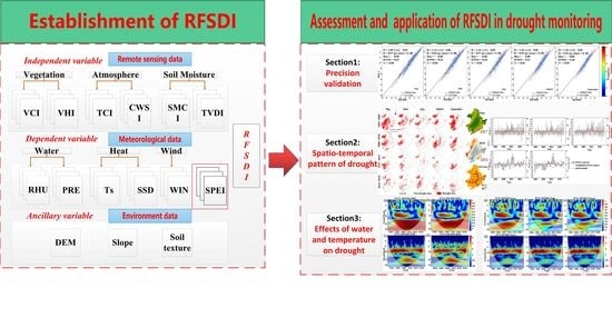
The actual observed SPEI was selected as the dependent variable. The temperature condition index (TCI), vegetation condition index (VCI), vegetation health index (VHI), temperature vegetation drought index (TVDI), crop water stress index (CWSI), and soil moisture condition index (SMCI) were used as independent variables. Terrain data and soil texture data were used as auxiliary variables.

(5)

The data were randomly divided into a test set (20%) and a training set (80%). Based on the BCRF model, different combinations of independent variables were introduced into the regression model to construct the model.

(6)

Model evaluation terms such as the R² and RMSE were used to evaluate the advantages and disadvantages of different combinations of independent variables when constructing the models to select the best regression model and construct the RFSDI.

2.4. Construction of Model-Building Parameters

2.4.1. Dependent Variable Construction

SPEI construction: The SPEI [10] is an index that calculates the difference between precipitation and reference evapotranspiration by introducing a probability model.

$$W=\left\{\begin{array}{c}\sqrt{-2\ln (P)},P\le 0.5\\ \sqrt{-2\ln (1-P)},P>0.5\end{array}\right.$$

(1)

$$SPEI=W-\frac{C_0+C_1\cdot W+C_2\cdot W^2}{1+d_1\cdot W+d_2\cdot W^2+d_3\cdot W^3}$$

(2)

where C₀, C₁, C₂, d₁, d₂, d₃ are constants, with values of 2.515517, 0.802853, 0.010328, 1.432788, 0.189269, and 0.001308, respectively. When p > 0.5, SPEI takes the opposite value.

2.4.2. Independent Variable Construction

TVDI construction: Sandholt et al. [33] proposed the concept of the TVDI, which is defined as follows.

$$\mathit{TVDI}=\frac{LS{T}_{VIi}-LS{T}_{VIi\min }}{LS{T}_{VIi\max }-LS{T}_{VIi\min }}$$

(3)

$$\begin{gathered} LST{}_{VIi\max }=a_1+b_{1}VIi \\ LST{}_{VIi\min } =a_2+b_{2}VIi \end{gathered}$$

(4)

where LSTVI, LST_VImin, and LST_VImax corresponding to time-series TVDI instantaneous value, minimum value, and maximum value, respectively; a₁, a₂, b₁, and b₂ are for the fitting equation coefficient.

VCI, TCI, VHI, SMCI, and CWSI [6,14,15] were calculated in this study based on the reconstructed EVI and LST for VCI, TCI, and VHI; soil moisture data were used for the SMCI; and ET and PET were also used for the CWSI.

$$\mathit{VCI}=\frac{EV{I}_{\max }-EV{I}_i}{EV{I}_{\max }-EV{I}_{\min }}$$

(5)

$$TCI=\frac{LS{T}_{\max }-LS{T}_i}{LS{T}_{\max }-LS{T}_{\min }}$$

(6)

$$\mathit{VHI}=a\times VCI+\left(1-a\right)\times TCI$$

(7)

$$SMCI=\frac{S{M}_i-S{M}_{\min }}{S{M}_{\max }-S{M}_{\min }}$$

(8)

$$CWSI=1-\frac{ET}{PET}$$

(9)

where i is the month, subscript max is the maximum value in the time series, and subscript min is the minimum value in the time series. In this study, a = 0.5 was adopted.

The above parameters were calculated in the ENVI + IDL programming environment.

2.5. Multiple Stepwise Regression Model

In this study, the RFSDI at the same time scale as the SPEI was calculated to analyze the multi-scale drought characteristics in NEC using a multiple linear regression model [20]. The regression equation was established, and the climatic variables and their standardized coefficients corresponding to the best model were determined, thereby clarifying the drought-dominated climatic variables and their direct effects on drought. The general expression of multiple stepwise regression is as follows.

$$Y=a_0+a_1{x}_1+a_2{x}_2+\cdots +a_n{x}_n+e$$

(10)

2.6. Time-Series Crossover Wavelet Model

In this study, the cross-wavelet transform was used to investigate the response time of agricultural drought to climate change [21]. The theoretical distribution formula of the cross-wavelet power of two time series can be expressed as follows.

$$D\left(\frac{\left|W_n^X\left(S\right)W_n^{Y^{\ast }}\left.\left(S\right)\right|\right.}{{\sigma }_X{\sigma }_Y}<p\right)=\frac{Z_v\left(p\right)}{v}\sqrt{P_k^X{P}_k^Y}$$

(11)

where ${\sigma }_X,{\sigma }_Y$ are the standard deviations of time series X_n and Y_n, respectively. When the background power spectrum is real wavelet v = 1 and complex wavelet v = 2, Z_v(p) is the confidence level of probability p.

The cross-wavelet phase angle a_m is defined as

$$a_m=\arg (X,Y)=\arg [{\displaystyle \sum }_{i=1}^N\cos a_i,{\displaystyle \sum }_{i=1}^N\sin a_i]$$

(12)

where a_i (i = 1, 2, …, N) is a single phase angle in the wavelet transform time domain.

3. Results

3.1. Accuracy of the BCRF Model

The BCRF regression model introduced different combinations of independent variables in this study. The optimal model was obtained based on the evaluation criteria of the model accuracy, and a regression equation was established.

Table 2. The optimal model and the better model.

Month	Independent Variable	R2		RMSE
		RF	BCRF	RF	BCRF
5	TVDI, CWSI, SMCI, TCI	0.85	0.88	0.30	0.28
6	TVDI, CWSI, SMCI, TCI, VCI, VHI	0.83	0.86	0.30	0.29
7	TVDI, CWSI, SMCI, VCI, VHI	0.82	0.87	0.32	0.30
8	TVDI, CWSI, SMCI, TCI, VCI, VHI	0.83	0.87	0.38	0.36
9	TVDI, CWSI, SMCI, TCI, VCI, VHI	0.83	0.89	0.39	0.37

presents the optimal model construction parameters in each month of the growing season, along with the model accuracy before and after the deviation correction model was applied. Overall, the accuracy and stability of the BCRF model were higher than those of the traditional RF model. The R² range of the optimal independent variable combination model optimized by the BCRF model was 0.86–0.89; this range was higher than those of the other independent variable combinations. The RMSE range was 0.28–0.37, which was lower than those of the other independent variable combinations. These results indicate that the accuracy of the regression model obtained by the BCRF model was better than that of the traditional model, thereby improving the model accuracy and enabling the construction of the RFSDI.

3.2. Assessment of the Drought-Monitoring Applicability and Drought-Monitoring Capability of the RFSDI

3.2.1. Applicability of the RFSDI_3 to Agricultural Drought Monitoring in Different Months

The optimal regression model was applied to multi-source data to obtain the monthly RFSDI_3 from 2003 to 2020. The actual observed SPEI_3 and corresponding RFSDI_3 for each period were extracted from meteorological stations, and the correlation analysis results are shown in Figure 3. The results indicate that the RFSDI_3 can effectively fit the measured SPEI_3, with R values above 0.95. The highest correlations between the RFSDI_3 and SPEI_3 were observed in May and June, with a correlation coefficient of 0.97. The RMSE values of the RFSDI_3 and observed SPEI_3 from May to September were all below 0.24, indicating that the RFSDI_3 can accurately identify drought in different months.

3.2.2. RFSDI Simulates the Drought Trends of Meteorological Stations in NEC

Figure 4 illustrates the drought change trends detected by the SPEI_3 and RFSDI_3 at two representative randomly selected meteorological stations in each of the four provinces (Hailun Station (50756) and Baoqing Station (50888) in Heilongjiang Province, Baicheng Station (50936) and Tongyu Station (54041) in Jilin Province, Zhangwu Station (54236) and Chaoyang Station (54324) in Liaoning Province, and Hailar Station (50527) and Tongliao Station (54135) in the Inner Mongolia Autonomous Region) from May to September during the 2003 to 2020 period. The RFSDI is highly consistent with the SPEI_3 and can accurately reflect the drought change trends in NEC. In addition, both the SPEI_3 and RFSDI_3 detected severe drought events (value ≤ −0.5) in 2003 to 2004 and 2017 to 2018, indicating that the RFSDI_3 can accurately capture the drought change trends in NEC. Moreover, the drought changes monitored by the RFSDI_3 and SPEI_3 were consistent, indicating that the RFSDI_3 can be utilized to evaluate the actual drought state by monitoring the occurrence of drought at different stations in the same month and the drought change trend at the same station.

3.2.3. Spatial Distribution of Drought Conditions in Typical Dry Years

To evaluate the drought identification ability of the RFSDI in different months, 2018 was selected as a typical drought year. The spatial distribution of drought stress (value ≤ −0.5) and non-drought stress (value > −0.5) [10] determined by the RFSDI in NEC from May to September 2018, as well as the actual SPEI_3 observations, are shown in Figure 5. The largest area experiencing drought stress in NEC was observed in May, when most of the region was affected by drought. The drought-stressed areas from June to September were concentrated in northwestern Heilongjiang Province and in the western and southern regions of Liaoning Province. In addition, Figure 5f shows the average drought identification ability of the RFSDI_3 from May–September, the growing season in NEC. The RFSDI_3 accuracy in identifying drought stress ranged from 85.5% to 100%. The accuracy of non-drought stress identification ranged from 81.1% to 100%. These results suggest that the RFSDI_3 has a high accuracy in identifying drought stress and non-drought stress, and the accuracy varies among different months.

The drought identification accuracies of the SPEI_3 and RFSDI_3 relative to the field survey data in agricultural areas in 2018 were calculated and are presented in

Table 3. Drought identification accuracy of SPEI_3 and RFSDI_3 relative to field survey.

Item		May		July		August
		SPEI	RFSDI	SPEI	RFSDI	SPEI	RFSDI
Accuracy (%)	Drought	83.30	100.00	66.67	100.00	68.42	77.78
	Non-drought	–	–	60.00	80.00	66.47	100.00

Note: The ‘–’ in the table means no area of this type.

. The results indicate that the RFSDI_3 has a higher accuracy in identifying drought than the SPEI_3. For identifying arid areas, the RFSDI_3 accuracies were 16.70%, 33.33%, and 9.36% higher than the SPEI_3 accuracies during the 3 field surveys. For identifying non-arid areas, the RFSDI_3 accuracies were 20.00% and 33.53% higher than the SPEI_3 accuracies in July and August, respectively.

3.3. Spatiotemporal Pattern of Drought in NEC Based on the RFSDI

The study period was divided into four periods, and the spatiotemporal pattern of drought in NEC based on the RFSDI was analyzed. Figure 6 shows the spatial distribution of agricultural drought in NEC during these periods. Overall, agricultural drought occurred during the growth period of the major grain crops, and the western part of the study area was more severely affected than the eastern part. Over the past 18 years, we observed slowing trends in the scope and intensity of agricultural drought in the study area.

Based on the RFSDI drought-monitoring results, the spatial distributions of the soil texture, elevation, and slope data were superimposed. The results show that the highest proportion of drought-affected areas occurred in loam and sandy soil areas. In contrast, drought occurred less frequently in clay areas. The highest percentages of drought-affected areas were at the elevation range of 50–300 m, while low-elevation areas such as the Sanjiang Plain below 50 m and high-elevation mountainous areas such as Baekdu Mountain and the Greater Khingan Mountains experienced less frequent drought conditions. Additionally, the highest percentage of drought-affected areas was in the 2–15° slope area.

3.4. Multi-Scale Characteristics of Drought from 2003 to 2020

Figure 7 displays the RFSDI changes under different time scales, as well as the corresponding cumulative percentage of precipitation anomalies and reference evapotranspiration anomalies. When using relatively long time scales (12 and 24 months), the RFSDI can effectively capture the drought characteristics and trends in NEC, and a stronger correlation was found between the RFSDI and the percentage of accumulated precipitation anomalies than between the RFSDI and the percentage of accumulated reference evapotranspiration anomalies. On relatively short time scales (1, 3, and 6 months), the RFSDI can accurately identify regional drought events. Overall, over the past 18 years, the severity of drought in NEC has undergone a cycle of approximately 10 years (RFSDI_24), with the duration and intensity of drought being greater in 2003 to 2010 than in 2010 to 2020. However, drought has occurred to some degree every year (RFSDI < 0). The drought frequency from 2010 to 2020 was higher than that from 2003 to 2010 (RFSDI_3).

3.5. Drought Dominates Climate Variables during the Growing Season

Table 4. Significance test for the mean of the growing season and the RFSDI_3 results from May to September in NEC.

Item	Month					Average Growth Season
	5	6	7	8	9
Shapiro–Wilk Sig.	0.506	0.694	0.299	0.531	0.208	0.416
Normal distribution (Y/N)	Y	Y	Y	Y	Y	Y

displays the results of the Shapiro−Wilk normalization test for the mean of the growing season and the RFSDI_3 results from May to September in the NEC region. The significance test results for the mean of each month and the growing season are greater than 0.05, which is close to a normal distribution and could be analyzed by stepwise linear regression.

Table 5. Optimal stepwise linear regression model and regression coefficients of RFSDI_3 and climate variables.

Month	Model Veriables	Model R2	Unstandardization Coefficient	Standardization Coefficient	Sig
May	(Constant)	0.962	−2.313	–	0.001
	PRE		0.011	0.668	0.008
	RHU		0.031	0.199	0.006
	Tmax		−0.033	−0.231	0.000
June	(Constant)	0.955	−1.150	–	0.000
	PRE		0.014	0.406	0.000
	RHU		0.048	0.166	0.004
	SSD		−0.101	−0.721	0.003
	Tmin		−0.120	−0.362	0.007
July	(Constant)	0.956	−5.398	–	0.000
	PRE		0.013	0.652	0.000
	RHU		0.106	0.626	0.001
	SSD		−0.401	−0.139	0.001
August	(Constant)	0.971	1.650	–	0.003
	PRE		0.027	0.413	0.006
	RHU		0.116	0.401	0.000
	Tmean		0.421	0.125	0.002
September	(Constant)	0.983	−4.417	–	0.000
	PRE		0.018	0.570	0.000
	RHU		0.058	0.550	0.000
	Tmax		−0.128	−0.265	0.002
Average growth season	(Constant)	0.944	−2.152	–	0.019
	PRE		0.021	0.556	0.000
	RHU		0.030	0.229	0.003
	Tmax		−0.053	−0.079	0.000
	SSD		0.177	0.243	0.001

displays the best stepwise linear regression model and regression coefficients of the RFSDI_3 and climate variables in the different months of the main growing season in NEC. The results demonstrate that the effects of climate variables on the RFSDI_3 differ among various months, and there are variations in the dominant climate variables of agricultural drought in different months. The average direct effect of PRE was the largest across different months and growing seasons, reaching 0.668, 0.406, 0.652, 0.413, 0.570, and 0.556 in each stage. Moreover, the direct effect of humidity on drought was second-largest in each stage, after only precipitation, reaching 0.199, 0.166, 0.626, 0.401, 0.550, and 0.229.

In Table 5, all the climate variables included in the best stepwise multiple regression model at each stage had a significance of <0.05, and the model was retained after interpretation. Moreover, all the included variables were drought-dominated climate variables at each stage.

The linear regression equation used to obtain the mean values from May–September and during the growing season based on stepwise multi-element regression is shown in

Table 6. Climate variables of different months of crop growing season and average drought in growing season based on multiple stepwise regression.

Month	Equation of Linear Regression
5	RFSDI_3May = −2.313 + 0.011PRE + 0.031RHU − 0.033Tmax
6	RFSDI_3June = −1.150 + 0.014PRE + 0.048RHU − 0.101SSD − 0.120Tmin
7	RFSDI_3July= −5.398 + 0.013PRE + 0.106RHU − 0.401SSD
8	RFSDI_3August= 1.650 + 0.027PRE + 0.116RHU + 0.421Tmean
9	RFSDI_3September= −4.417 + 0.018PRE + 0.058RHU − 0.128Tmax
Growth season	RFSDI_3Growth= −2.152 + 0.021PRE + 0.030RHU + 0.177SSD − 0.053Tmax

.

3.6. Effects of Water Stress on Agricultural Drought in NEC

Figure 8 displays the wavelet power spectra for the two types of moisture variables and RFSDI, as well as the condensation spectrum. As seen in Figure 8a, two distinct resonance periods of 10–16 months occur between PRE and the RFSDI during 2007 to 2012 and 2019 to 2020. The phase relationship during the former period shows a positive correlation between PRE and the RFSDI with a lag time of approximately 1.5 months. In contrast, the phase relationship during the latter period shows a negative correlation between PRE and the RFSDI with a lag time of approximately 3 months. Figure 8c demonstrates that 2 distinct resonance periods of 10–14 months occur between RHU and the RFSDI during 2006 to 2011 and 2019 to 2020. The phase relationship during the former period shows a positive correlation between RHU and the RFSDI with a lag time of approximately 3 months. In contrast, the phase relationship during the latter period shows a negative correlation with a lag time of approximately 4.5 months. Additionally, from 2005 to 2020, a resonance period of approximately 16–64 months occurs between the 2 moisture variables and RFSDI, with a positive correlation. Figure 8b,d display a resonance period of 10–14 months between the 2 types of moisture variables and RFSDI, with the phase relationship transitioning from a positive correlation to a negative correlation. The resonance period between PRE and the RFSDI spans from 2003 to 2020, with a lag of 1.5–4.5 months. The resonance periods between RHU and the RFSDI occur in 2003 to 2013 and 2015 to 2020, respectively, with lags of 1.5–4.5 months.

In Figure 9a–c, two 10–12-month resonance periods are observed between the 3 types of temperature variables and RFSDI during 2006 to 2015 and 2018 to 2020. Significant positive correlations are found between the 3 types of temperature variables and the RFSDI from 2006 to 2015, with a lag time of approximately 1.5 months. In contrast, there are significant negative correlations between the 3 types of temperature variables and RFSDI during 2018 in 2020, with a lag time of approximately 3 months. Moreover, there is a discontinuous 32–64-month resonance period between the 3 types of temperature variables and the RFSDI during 2003 to 2020. Among the three types of temperature variables, Tmax displays better continuity and duration, indicating that Tmax is more strongly associated with drought induction than the other two types of temperature variables to some extent. According to Figure 9d–f, resonance periods of 8–16 months are found between the 3 types of temperature variables and RFSDI from 2003 to 2020, with lag times ranging from 1.5 months to 3 months.

4. Discussion

4.1. RFSDI Construction Variable Selection Principle and Drought Identification Accuracy

The occurrence of agricultural drought is the result of the cooperative action of disaster-prone environment, disaster-causing factors, and disaster-bearing bodies. From the perspective of interaction between disaster factors and vegetation, rising air temperature aggravated soil water evaporation and vegetation transpiration loss, resulting in decreased soil water, and vegetation was characterized by drought [18]. In terms of the interaction between vegetation and disaster-prone environment, the soil conditions in NEC are sandy and loam soil, and the soil water retention ability is poor. Vegetation responds to the water shortage caused by these conditions, which are characterized by drought. From the interaction between disaster factors and disaster-prone environment, soil texture and slope conditions in drought-prone areas easily cause soil erosion, which leads to soil and water loss, and thus, vegetation is characterized by drought [34]. It can be seen that the complex synergistic relationship among disaster-causing factors, disaster-causing environment, and vegetation leads to the occurrence of drought. Therefore, the RFSDI constructed in this study considered the synergistic relationship among disaster-causing factors, disaster-causing environment, and disaster-bearing bodies, and it comprehensively considered atmospheric factors, disaster-bearing body factors, and soil topographic background conditions. In addition, this study shows (Figure 8 and Figure 9) that the cumulative effects of temperature, precipitation, and agricultural drought have a lag of 1.5–3 months and 1.5–4.5 months. Therefore, it is reasonable to select 3-month SPEI as an independent variable, which can better fit agricultural drought and meteorological drought.

This study not only verified the drought identification ability of the RFSDI using actual meteorological data but also validated the drought identification accuracy of the RFSDI using field survey data collected in 2018 (Table 3). The results show that the RFSDI had a higher drought-monitoring accuracy and stronger SPEI identification ability than other indices. The new drought index constructed in this study can accurately identify the occurrence of agricultural drought. In addition, climate change also causes periodic changes in climate variables such as temperature and precipitation [2], which in turn leads to periodic changes in drought, which is consistent with the conclusions of this study (Figure 7).

In addition, we also analyzed the correlation between the SPI_3 and RFSDI_3 to further verify the drought identification accuracy of RFSDI. The results in Figure 10 show that the correlation between the SPI_3 and RFSDI_3 in the growing season of crops was greater than 0.908, which could accurately identify agricultural drought.

4.2. Spatiotemporal Pattern of Drought in NEC Based on the RFSDI

Previous studies have investigated the drought trend in NEC by using remote sensing and meteorological indices [35,36]. Based on the drought-monitoring results of the RFSDI, this study divided the study period into four periods and analyzed the spatial and temporal patterns of drought in NEC (Figure 6).

The results show that the drought conditions in NEC included serious spring droughts, summer droughts that decelerated compared to the spring droughts, and autumn droughts that intensified again. These findings are consistent with the study by Zhang et al. [37] of NEC’s climate change characteristics. Agriculture droughts in NEC are distributed mainly in the central plains, where the elevation is mostly concentrated below 300 m, the slope is below 15°, and the soil texture is mainly loam and sand. The essence of agricultural drought is that long-term extreme climate conditions lead to a decreased soil moisture content, thereby limiting crop growth. The soil clay−sand ratio, slope size, and elevation conditions also directly affect the soil moisture conservation ability [36]. Based on the RFSDI agricultural drought-monitoring results, the study superimposed the spatial distribution data of soil texture, elevation, and slope to explore the occurrence of drought in different underlying surface environments (Figure 6). The soil water losses in agricultural areas with slopes below 2° were not severe, and the soil water contents were high. Agricultural drought in NEC occurred mainly in low-elevation sloping farmlands. The precipitation in areas with slopes greater than 15° was more abundant than that in the central plain area, and the temperature was lower than that in the plain area at the same time. In addition, abundant snow and ice meltwater in the spring season in areas with forest land cover types contributed to relatively high soil moisture in such areas, making them less susceptible to drought stress.

This study suggests that the differences in the spatiotemporal distribution of drought within the NEC region are not caused solely by differences in moisture and temperature but are also caused by differences in soil texture and topography. Previous research on drought at the county scale [36] demonstrated that differences in slope, elevation, and soil texture directly led to spatial differences in drought occurrence, with slope changes resulting in the most severe soil moisture losses. Based on our agricultural-drought-monitoring results, we discussed the spatial and temporal patterns and causes of agricultural drought in NEC at a large regional scale, and our conclusions were consistent with the research results of Du et al. [35].

4.3. Drought in Different Agricultural Areas in NEC

Due to differing terrain and climatic conditions, drought trends vary among different agricultural areas of NEC. Therefore, this study analyzed the drought trends in eight agricultural regions based on previous agricultural zoning results obtained in NEC [28]. Figure 11 shows the drought change trends in these 8 regions over the past 18 years. Generally, drought in the Greater Khingan Mountains, the Lesser Khingan Mountains, the Sanjiang Plain, the Songnen Plain, the Hulunbeier Grassland, and the Western Liao River has shown a slowing trend, while drought in the Liaoning Plain and hilly zone and Baekdu Mountain has shown an increasing trend. Among these areas, the most obvious drought enhancement trend was found in Baekdu Mountain, and the most obvious drought mitigation trend was observed in the Lesser Khingan Mountains. This study found that the mean temperature during the growing season in the Baekdu Mountain area shows an increasing trend, while precipitation shows a decreasing trend; these changes were opposite in the Lesser Khingan Mountains area. Therefore, the changes in temperature and precipitation and the differences in their spatial and temporal distributions are the main reasons for the different drought change trends observed in different agricultural areas in NEC. Under the combined influence of topographic factors such as the surface coverage type, soil water retention, elevation, and slope in different agricultural areas, the drought change trend varies.

Despite the overall slowing drought trend observed in NEC over the past 18 years, there are still regional differences in the drought change trends. Therefore, it is necessary to pay attention to the drought change trend in drought-prone areas such as the Liaoning Plain and hilly zone and Baekdu Mountain and take certain drought prevention measures to reduce losses caused by drought. In addition, drought and waterlogging disasters are two extreme water stress phenomena, and drought mitigation has led to an increased frequency of waterlogging disasters to a certain extent. Hence, it is crucial to pay attention to the possibility of waterlogging disasters in significantly drought-mitigated areas such as the Sanjiang Plain and the Songnen Plain.

4.4. Effects of Climate Change on Agricultural Drought in NEC

Agricultural drought is caused by the continuous occurrence of extreme climate conditions, so agricultural drought and meteorological drought also have a certain lag time [38]. Therefore, it is important to determine the relationships between agricultural drought and climate variables. Figure 12 shows the change trends in 6 climate variables over the last 18 years. The 6 variables show upwards trends, with PRE having the most significant increasing trend of 6.12 mm/10 a. The change trends in SSD, RHU, Tmean, Tmin, and Tmax are 0.23 h/10 a, 0.09 mm/10 a, 0.15 °C/10 a, 0.25 °C/10 a, and 0.21 °C/10 a, respectively. Overall, under the influence of these climate variables, drought in the last 18 years shows a slowing trend. This study also found that the drought change in NEC showed a cycle of approximately 10 years.

From 2003 to 2010, Tmin, Tmax, Tmean, PRE, and SSD showed downwards trends, with change trends of −0.89 °C/10 a, −1.15 °C/10 a, −0.99 °C/10 a, −1.09 mm/10 a, and −0.15 h/10 a, respectively, while RHU showed an upwards trend, with a change trend of 1.66 mm/10 a. From 2010 to 2020, Tmin, Tmax, Tmean, PRE, and SSD showed upwards trends, with change trends of 1.32 °C/10 a, 1.75 °C/10 a, 1.57 °C/10 a, 8.41 mm/10 a, and 0.85 h/10 a, respectively, while RHU showed a downwards trend, with a change trend of −3.72 mm/10 a.

From a numerical perspective, the trends in the aforementioned climate variables may suggest lighter drought from 2003 to 2010 and heavier drought from 2010 to 2011. However, there is a lag time between meteorological drought and agricultural drought, and the latter is caused by the accumulation of long-term extreme weather conditions. Considering previous research on the lag time between meteorological and agricultural drought [39], this study proposes that the overall light drought observed from 2010 to 2020 was due to the accumulation of climate change in the earlier period. Conditions that were not conducive to drought occurred from 2003 to 2010, with Ts, PRE, and SSD showing downwards trends and RHU showing a slight upwards trend, indicating that these climate variables were moving towards conditions that were not favorable for drought. Therefore, the agricultural drought between 2010 and 2020 was generally milder. Similarly, the heavy drought from 2003 to 2010 may have been a result of conditions favorable to drought occurring from 1990 to 2000, with the incubation period and outbreak of agricultural drought completed from 1990 to 2000. Hence, the period of agricultural drought between 2003 and 2010 was the outbreak and persistence period, resulting in generally heavier drought during this time.

In other words, between 2010 and 2020, Ts, PRE, and SSD showed clear upwards trends, while RHU showed a slight downwards trend. The changing trends in these climatic variables favored the occurrence of drought, yet the drought during this period was generally relatively mild. This does not exclude the possibility of an incubation or outbreak period for the next heavy drought. This is consistent with the research results of Zhang et al. [27]. This study suggests that drought in NEC increased from 2003 to 2010 but showed a slowing trend from 2011 to 2020. Over the past 18 years, drought in NEC has generally shown a slowing trend, displaying a cyclical change of almost 10 years (Figure 6). Although there are some differences between this study and previous research regarding the drought indices used, the conclusion on the drought evolution trend is reasonable when considering the trends in climate variables within the study period. Therefore, we should remain vigilant in drought-prone areas in the next decade and implement appropriate irrigation measures to reduce the impacts of drought on the healthy growth and yield of food crops.

In addition, the dominant climate variables of agricultural drought in crop growing season are also different (Table 5 and Table 6), which is also related to the climatic factors in Northeast China. In spring, the Northeast China warms up rapidly, but the precipitation is insufficient, and it is difficult for the glacier meltwater in the mountainous area to reach the central arable area, which makes the arable area prone to drought. In summer, the temperature in Northeast China is higher, but the precipitation is also abundant, so the drought is alleviated compared with spring. In autumn, the precipitation in this area decreased, but the temperature did not decrease significantly. At this time, the crops entered the harvest period, and the underlying surface gradually turned to the period of low vegetation coverage. In addition, under the influence of a monsoon, the loss of soil moisture accelerated, which made the decrease in soil moisture content more obvious and then showed the characteristics of drought. It can be seen that under the influence of climate change, the dominant climate variables of agricultural drought in crop growing season in Northeast China are different, but precipitation and temperature are still the most important disaster-causing factors in agricultural drought.

5. Conclusions

Using multi-source data, this study comprehensively considered the interactions among factors that cause disasters, the environmental conditions that lead to disaster, and the bodies that bear the disaster. In addition, this study added the environmental conditions of drought occurrence and post-disaster vegetation status information and constructed the RFSDI using a deviation-correction random forest model. The ability and accuracy of the index for drought identification in NEC were evaluated by comparing the index results with the actual observed SPEI and field survey data in 2018. Based on the developed index, the spatial and temporal patterns of agricultural drought in NEC and the dominant climate variables of agricultural drought in the growing season were discussed. This study drew the following conclusions:

(1)

The RFSDI constructed in this study has a high degree of fit with the actual observed SPEI and field drought survey data, accurately describing the spatial and temporal patterns of and evolution trend in agricultural drought in NEC and identifying drought-stressed areas.

(2)

From 2003 to 2020, the influence range of spring drought in NEC was the widest, the summer drought weakened, and the autumn drought increased again. The central and western plains of the study area were most seriously affected by drought stress due to the combined action of disaster-causing factors and disaster-prone environments.

(3)

From 2003 to 2020, the overall drought in NEC showed a slowing trend. Due to the influence of climate and geographical factors, the trend in drought in different agricultural areas varied. From an interannual perspective, the agricultural drought in NEC exhibited cyclical changes of nearly 10 years.

(4)

The dominant climate variables affecting agricultural drought during the growing season included PRE, Ts, RHU, and SSD. A significant correlation was found between the changes in water and heat and the occurrence of agricultural drought in NEC. A lag of 1.5–4.5 months was found between the decrease in precipitation and soil moisture and the occurrence time of agricultural drought.

References

1. Wang, X.; Pan, S.; Pan, N.; Pan, P. Grassland productivity response to droughts in northern China monitored by satellite-based solar-induced chlorophyll fluorescence. J. Sci. Total Environ. 2022, 830, 154550. [Google Scholar] [CrossRef] [PubMed]
2. Xie, N.; Xin, J.; Liu, S. China’s regional meteorological disaster loss analysis and evaluation based on grey cluster model. Nat. Hazards 2014, 71, 1067–1089. [Google Scholar] [CrossRef]
3. Qin, Y.; Xiao, X.; Wigneron, J.-P.; Ciais, P.; Canadell, J.G.; Brandt, M.; Li, X.; Fan, L.; Wu, X.; Tang, H.; et al. Large loss and rapid recovery of vegetation cover and aboveground biomass over forest areas in Australia during 2019–2020. Remote Sens. Environ. 2022, 278, 113087. [Google Scholar] [CrossRef]
4. Zhang, J. Risk assessment of drought disaster in the maize-growing region of Songliao Plain, China. J. Agric. Ecosyst. Environ. 2004, 102, 133–153. [Google Scholar] [CrossRef]
5. Wasti, S.; Wang, Y. Spatial and temporal analysis of HCHO response to drought in South Korea. J. Sci. Total Environ. 2022, 852, 158451. [Google Scholar] [CrossRef]
6. Song, Y.; Fang, S.; Yang, Z.; Shen, S. Drought indices based on MODIS data compared over a maize-growing season in Songliao Plain, China. J. Appl. Remote Sens. 2018, 12, 046003. [Google Scholar] [CrossRef]
7. Basit, A.; Ni, J.; Khan, F.U.; Sajid, M.; Umair, M.; Makanda, T.A. Impact assessment of drought monitoring events and vegetation dynamics based on multi-satellite remote sensing data over Pakistan. J. Environ. Sci. Pollut. Res. 2023, 30, 12223–12234. [Google Scholar] [CrossRef]
8. Tian, Y.; Yang, Y.; Bao, Z.; Song, X.; Wang, G.; Liu, C.; Wu, H.; Mo, Y. An Analysis of the Impact of Groundwater Overdraft on Runoff Generation in the North China Plain with a Hydrological Modeling Framework. J. Water 2022, 14, 1758. [Google Scholar] [CrossRef]
9. Fu, R.; Chen, R.; Wang, C.; Chen, X.; Gu, H.; Wang, C.; Xu, B.; Liu, G.; Yin, G. Generating High-Resolution and Long-Term SPEI Dataset over Southwest China through Downscaling EEAD Product by Machine Learning. J. Remote Sens. 2022, 14, 1662. [Google Scholar] [CrossRef]
10. Vicente-Serrano, S.M.; Beguería, S.; López-Moreno, J.I. A Multiscalar Drought Index Sensitive to Global Warming: The Standardized Precipitation Evapotranspiration Index. J. Clim. 2010, 23, 1696–1718. [Google Scholar] [CrossRef]
11. Uddin, M.J.; Hu, J.; Islam, A.R.M.T.; Eibek, K.U.; Nasrin, Z.M. A comprehensive statistical assessment of drought indices to monitor drought status in Bangladesh. J. Arab. J. Geosci. 2020, 13, 323. [Google Scholar] [CrossRef]
12. Liu, X.; Guo, P.; Tan, Q.; Xin, J.; Li, Y.; Tang, Y. Drought risk evaluation model with interval number ranking and its application. J. Sci. Total Environ. 2019, 685, 1042–1057. [Google Scholar] [CrossRef]
13. Qiao, L.; Qian, H.; Di Huo, A. A Review of Remote Sensing Drought Monitoring Method. J. Adv. Mater. Res. 2015, 1073–1076, 1891–1894. [Google Scholar] [CrossRef]
14. Kogan, F. World droughts in the new millennium from AVHRR-based vegetation healthindices. J. Eos Trans. Am. Geophys. Union 2002, 83, 557–563. [Google Scholar] [CrossRef]
15. Hu, X.; Ren, H.; Tansey, K.; Zheng, Y.; Ghent, D.; Liu, X.; Yan, L. Agricultural drought monitoring using European Space Agency Sentinel 3A land surface temperature and normalized difference vegetation index imageries. J. Agric. For. Meteorol. 2019, 279, 107707. [Google Scholar] [CrossRef]
16. Guo, H.; Bao, A.; Ndayisaba, F.; Liu, T.; Jiapaer, G.; El-Tantawi, A.M.; De Maeyer, P. Space-time characterization of drought events and their impacts on vegetation in Central Asia. J. Hydrol. 2018, 564, 1165–1178. [Google Scholar] [CrossRef]
17. Merino, A.; López, L.; Hermida, L.; Sánchez, J.L.; García-Ortega, E.; Gascón, E.; Fernández-González, S. Identification of drought phases in a 110-year record from Western Mediterranean basin: Trends, anomalies and periodicity analysis for Iberian Peninsula. J. Glob. Planet. Chang. 2015, 133, 96–108. [Google Scholar] [CrossRef]
18. Qutbudin, I.; Shiru, M.S.; Sharafati, A.; Ahmed, K.; Al-Ansari, N.; Yaseen, Z.M.; Shahid, S.; Wang, X. Seasonal Drought Pattern Changes Due to Climate Variability: Case Study in Afghanistan. J. Water 2019, 11, 1096. [Google Scholar] [CrossRef]
19. Leng, G.; Hall, J. Crop yield sensitivity of global major agricultural countries to droughts and the projected changes in the future. Sci. Total Environ. 2019, 654, 811–821. [Google Scholar] [CrossRef]
20. Kumar, K.A.; Reddy, G.O.; Masilamani, P.; Turkar, S.Y.; Sandeep, P. Integrated drought monitoring index: A tool to monitor agricultural drought by using time series datasets of space-based earth observation satellites. J. Adv. Space Res. 2021, 67, 298–315. [Google Scholar] [CrossRef]
21. Anyamba, A.; Small, J.L.; Tucker, C.J.; Pak, E.W. Thirty-two Years of Sahelian Zone Growing Season Non—Stationary NDVI3g Patterns and Trends. J. Remote Sens. 2014, 6, 3101–3122. [Google Scholar] [CrossRef]
22. Zhu, K.; Ying, L. Information Source Detection in the SIR Model: A Sample-Path-Based Approach. J. IEEE/ACM Trans. Netw. 2014, 24, 408–421. [Google Scholar] [CrossRef]
23. Wu, Q.; Zhong, R.; Zhao, W.; Song, K.; Du, L. Land-cover classification using GF-2 images and airborne lidar data based on random forest. J. Int. J. Remote Sens. 2018, 40, 2410–2426. [Google Scholar] [CrossRef]
24. Li, C.; Adu, B.; Wu, J.; Qin, G.; Li, H.; Han, Y. Spatial and temporal variations of drought in sichuan province from 2001 to 2020 based on modified temperature vegetation dryness index (tvdi)Sciencedirect. J. Ecol. Indic. 2022, 139, 108883. [Google Scholar] [CrossRef]
25. Brown, J.F.; Wardlow, B.D.; Tadesse, T.; Hayes, M.J.; Reed, B.C. The Vegetation Drought Response Index (VegDRI): A New Integrated Approach for Monitoring Drought Stress in Vegetation. J. GiSci. Remote Sens. 2008, 45, 16–46. [Google Scholar] [CrossRef]
26. Zhang, Q.; Shi, R.; Xu, C.-Y.; Sun, P.; Yu, H.; Zhao, J. Multisource data-based integrated drought monitoring index: Model development and application. J. Hydrol. 2022, 615, 128644. [Google Scholar] [CrossRef]
27. Zhang, Q.; Yu, H.; Sun, P.; Singh, V.P.; Shi, P. Multisource data based agricultural drought monitoring and agricultural loss in China. J. Glob. Planet Chang. 2019, 172, 298–306. [Google Scholar] [CrossRef]
28. Wan, W.; Liu, Z.; Li, B.; Fang, H.; Wu, H.; Yang, H. Evaluating soil erosion by introducing crop residue cover and anthropogenic disturbance intensity into cropland C-factor calculation: Novel estimations from a cropland-dominant region of Northeast China. J. Soil Tillage Res. 2022, 219, 105343. [Google Scholar] [CrossRef]
29. Hao, P.; Zhan, Y.; Wang, L.; Niu, Z.; Shakir, M. Feature Selection of Time Series MODIS Data for Early Crop Classification Using Random Forest: A Case Study in Kansas, USA. Remote Sens. 2015, 7, 5347–5369. [Google Scholar] [CrossRef]
30. Duan, Y.; Zhong, J.; Shuai, G.; Zhu, S.; Gu, X. Time-scale transferring deep convolutional. Neural network for mapping early rice. In Proceedings of the C. IGARSS 2018—2018 IEEE International Geoscience and Remote Sensing Symposium, Valencia, Spain, 22–27 July 2018. [Google Scholar]
31. Hijmans, R.J.; Cameron, S.E.; Parra, J.L.; Jones, P.G.; Jarvis, A. Very high resolution interpolated climate surfaces for global land areas. J. Int. J. Climatol. 2005, 25, 1965–1978. [Google Scholar] [CrossRef]
32. Song, J. Bias corrections for Random Forest in regression using residual rotation. J. Korean Stat. Soc. 2015, 44, 321–326. [Google Scholar] [CrossRef]
33. Sandholt, I.; Rasmussen, K.; Andersen, J. A simple interpretation of the surface temperature/vegetation index space for assessment of surface moisture status. J. Remote Sens. Environ. 2002, 79, 213–224. [Google Scholar] [CrossRef]
34. Nabaei, S.; Sharafati, A.; Yaseen, Z.M.; Shahid, S. Copula based assessment of meteorological drought characteristics: Regional investigation of Iran. J. Agric. For. Meteorol. 2019, 276–277, 107611. [Google Scholar] [CrossRef]
35. Du, L.; Song, N.; Liu, K.; Hou, J.; Hu, Y.; Zhu, Y.; Wang, X.; Wang, L.; Guo, Y. Comparison of Two Simulation Methods of the Temperature Vegetation Dryness Index (TVDI) for Drought Monitoring in Semi-Arid Regions of China. J. Remote Sens. 2017, 9, 177. [Google Scholar] [CrossRef]
36. Ranzi, R.; Caronna, P.; Tomirotti, M. Impact of climatic and land use changes on river flows in the Southern Alps. In Sustainable Water Resources Planning and Management Under Climate Change; Springer: Berlin/Heidelberg, Germany, 2017; pp. 61–83. [Google Scholar]
37. Zhang, Q.; Hu, Z. Assessment of drought during corn growing season in Northeast China. J. Theor. Appl. Clim. 2018, 133, 1315–1321. [Google Scholar] [CrossRef]
38. Yan, H.; Zhou, G.; Yang, F.; Lu, X. DEM correction to the TVDI method on drought monitoring in karst areas. Int. J. Remote Sens. 2019, 40, 2166–2189. [Google Scholar] [CrossRef]
39. Wu, D.H.; Zhao, X.; Liang, S.L.; Zhou, T.; Huang, K.C.; Tang, B.J.; Zhao, W.Q. Time-lag effects of global vegetation responses to climate change. J. Glob. Chang. Biol. 2015, 21, 3520–3531. [Google Scholar] [CrossRef]
Figure 1. Overview of the study area: (a) location of the study region in China; (b) spatial distribution of annual cumulative precipitation; (c) spatial distribution of annual mean temperature; (d) DEM and meteorological observation stations; and (e) spatial pattern of upland and upland fields and agricultural zoning. Note: SJP, Sanjiang Plain Zone; GKM, Greater Khingan Mountain Zone; LKM, Lesser Khingan Mountain Zone; BM, Baekdu Mountain Zone; SNP, Songnen Plain Zone; WLR, Western Liao River Zone; HG, Hulunbuir Grassland Zone; LPH, Liaoning Plain and Hilly Zone.
Remotesensing 15 02477 g001
Figure 2. Model construction flow chart of RFSDI.
Remotesensing 15 02477 g002
Figure 3. Correlation analysis between RFSDI and SPEI_3.
Remotesensing 15 02477 g003
Figure 4. Drought trends of SPEI_3 and RFSDI_3 at typical sites.
Remotesensing 15 02477 g004
Figure 5. Drought-stressed areas identified by RFSDI and actual observations by SPEI_3 in (a) May (b) June (c) July (d) August (e) September and (f) average drought identification ability.
Remotesensing 15 02477 g005
Figure 6. Spatial distribution of agricultural drought, temperature, moisture, and slope in NEC.
Remotesensing 15 02477 g006
Figure 7. Cumulative precipitation anomaly and cumulative reference evapotranspiration anomaly of RFSDI at different time scales and corresponding scales.
Remotesensing 15 02477 g007
Figure 8. (a,b) wavelet power spectrum, (c,d) condensation spectrum of water stress variables.
Remotesensing 15 02477 g008
Figure 9. (ac) wavelet power spectrum, (df) condensation spectrum of temperature stress variables.
Remotesensing 15 02477 g009
Figure 10. The correlation between SPI_3 and RFSDI_3 in crop growth season.
Remotesensing 15 02477 g010
Figure 11. Variation trend in drought in different agricultural areas in NEC.
Remotesensing 15 02477 g011
Figure 12. Agricultural drought dominated the change trend in climate variables in NEC in the last 18 years. The ‘RED line’ represents the trend of climate variables during 2003 in 2020, while the ‘BLUE line’ represents the drought trend from 2003 to 2010 and 2011 to 2020.
Remotesensing 15 02477 g012