Abstract
The Visible Infrared Imaging Radiometer Suite Day/Night Band (VIIRS/DNB) nighttime light data is a powerful remote sensing data source. However, due to stray light pollution, there is a lack of VIIRS data in mid-high latitudes during the summer, resulting in the absence of high-precision spatiotemporal continuous datasets. In this paper, we first select nine-time series interpolation methods to interpolate the missing images. Second, we construct image pixel-level temporal continuity constraints and spatial correlation constraints and remove the pixels that do not meet the constraints, and the eliminated pixels are filled with the focal statistics tool. Finally, the accuracy of the time series interpolation method and the spatiotemporally constrained interpolation method (STCIM) proposed in this paper are evaluated from three aspects: the number of abnormal pixels (NP), the total light brightness value (TDN), and the absolute value of the difference (ADN). The results show that the images simulated by the STCIM are more accurate than the nine selected time series interpolation methods, and the image interpolation accuracy is significantly improved. Relevant research results have improved the quality of the VIIRS dataset, promoted the application research based on the VIIRS DNB long-time series night light remote sensing image, and enriched the night light remote sensing theory and method system.
1. Introduction
Nighttime light has important application value in the research and development of remote sensing applications. As a technology different from traditional optical remote sensing or microwave remote sensing, it uses earth observation sensors to obtain visible light-near-infrared electromagnetic wave information emitted by the Earth’s surface under cloudless conditions at night, providing a unique and direct perspective for human social activities [1], and is widely used in the fields of population spatialization estimation [2,3,4,5], socioeconomic evaluation [6,7,8], and ecological environment and urbanization process assessment [9,10,11,12,13,14,15]. The Visible Infrared Imaging Radiometer Suite (VIIRS) onboard the Suomi National Polar-Orbiting Partnership Satellite (S-NPP) provides a new generation of nighttime light remote sensing data. Compared with the stable nighttime light dataset acquired by the Defense Meteorological Satellite Program/Operational Linescan System (DMSP/OLS), the VIIRS data have been significantly improved and are more developed in terms of radiation accuracy, spatial resolution, and geometric quality, which further expands the research direction and application field of nighttime light remote sensing [16,17,18,19,20]; thus, these data are currently attracting the attention of an increasing number of researchers and are being widely applied [21,22,23,24,25]. Accessible, continuous monthly and annual synthetic nighttime light datasets are essential for applied research in various fields.
The National Oceanic and Atmospheric Administration (NOAA) has released vcm (VIIRS Cloud Mask) and vcmsl (VIIRS Cloud Mask Stray Light) monthly DNB synthetic data products at the National Geophysical Data Center (NGDC) since 2014. Due to stray light pollution, the monthly synthetic data of VIIRS DNB vcm in mid-high latitudes during the summer are highly distorted. These data exclude all pixels affected by stray light, resulting in many missing values and discontinuities in both space and time. The vcmsl product corrects the pollution data according to the stray light correction method proposed by Mills (2013) et al. [26] and retains more data in the mid-high latitudes in summer, but the overall data quality of this product is reduced. The currently released corrected VIIRS DNB annual synthetic nighttime light data contain two versions, V1 and V2. The V1 version data only include two periods: 2015 and 2016. This dataset was produced only using vcm data, not any other data affected by stray light, excluding the effects of short-lived lights and nonlight signals. The V2 version data contain continuous annual synthetic data from 2012 to 2021, which are based on the vcmsl monthly synthetic dataset [27]. However, due to defects in the stray light removal process of the vcmsl dataset, the method still retains the problem that noise cannot be removed in the high latitudes of the Northern Hemisphere. The lack of high-precision, spatiotemporally continuous datasets is becoming a significant obstacle to advancing the in-depth application of VIIRS DNB monthly and annual synthetic data.
In response to the above problems, some scholars have researched the interpolation and synthesis of missing pixels in VIIRS DNB data. Zhao et al. used monthly VIIRS DNB data to evaluate US GDP economic indicators and used the single exponential smoothing method to interpolate the missing values of vcm data [28]. Chen et al. conducted a comparative study on the VIIRS DNB monthly product data interpolation method using Beijing as an example and systematically compared the applicability of four interpolation methods in terms of abnormal interpolation values, reference values, and computational performance, namely cubic spline interpolation, cubic Hermite interpolation, gray model, and three exponential smoothing model [29]. Fan et al. conducted a comparative study on the interpolation of VIIRS/DNB night light remote sensing data for cities of different scales worldwide based on eight methods: least squares linear fitting, least squares quadratic polynomial fitting, least squares cubic polynomial fitting, cubic bezier curve interpolation, gray forecasting model, cubic spline interpolation, cubic exponential smoothing, and cubic Hermite Interpolation [30]. The above attempts focus on establishing a mathematical model from the perspective of the time continuity of multiple months at a single pixel location and carrying out fitting and approximation simulations to calculate the pixel value of the missing month. However, such methods do not consider the relative stability of the urban spatial structure, the relative stability of the luminous time series of the same objects, or the spatial correlation between data pixels in the same month. Therefore, there is still much room in the current interpolation methods for missing image pixel values in the VIIRS dataset.
Therefore, in this paper, we propose a STCIM that considers temporal continuity, the relative stability of the urban spatial structure, and the relative smoothness of the night light of the same objects in time. Moreover, we chose the direct replacement method (DR), least squares linear fitting method (LSM), least squares quadratic polynomial fitting (LSM2), least squares cubic polynomial fitting (LSM3), cubic spline interpolation (Spline), cubic Bezier curve interpolation (Bezier), gray forecasting model (GFM), cubic exponential smoothing (Exponent), and cubic Hermite Interpolation (Hermite) methods. Nine kinds of widely used time series interpolation methods were compared and analyzed. Taking Shanghai as an example, the images of Shanghai for June of each year were simulated. The accuracy of the time series interpolation and STCIM results were evaluated in terms of NP, TDN, and ADN. We also analyzed whether the STCIM, with temporal and spatial relationships as constraints on each other, is more accurate than the time series interpolation method with temporal relationships as constraints. This research is necessary to obtain monthly synthetic and annual synthetic night light datasets of VIIRS DNB with spatiotemporal continuity and higher accuracy. It is also crucial to enrich the theoretical and methodological system of night light remote sensing and broaden the application value of night light remote sensing images based on the VIIRS DNB long-time series.
2. Study Area and Data
2.1. Study Area
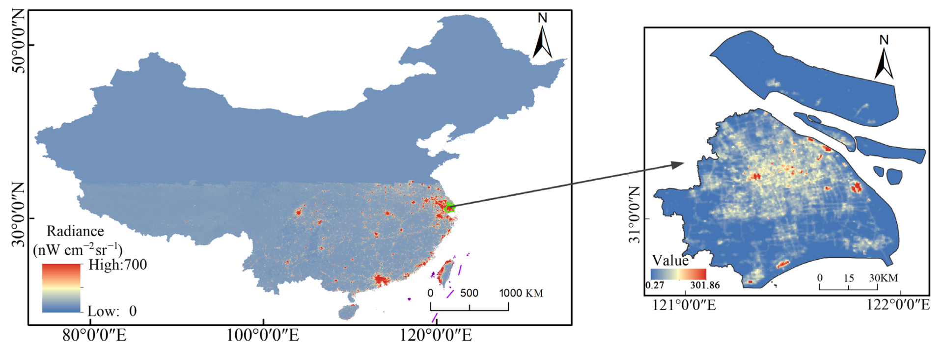
Shanghai, located at 120°52′E–122°12′E, 30°40′N–31°53′N, at mid-latitude in the Northern Hemisphere, is a municipality directly under the Central Government of the People’s Republic of China, a national central city, and an international center of economy, finance, trade, shipping, science and innovation (Figure 1). At the end of 2021, Shanghai’s resident population was 24.8943 million, ranking second in China’s urban resident population. In 2021, Shanghai’s regional GDP was 4321.485 billion yuan, ranking first in China’s urban GDP. Nighttime light data can be applied to population spatialization estimation and socioeconomic assessment. However, because Shanghai is located in the middle latitude of the Northern Hemisphere, the VIIRS nighttime light data in summer are missing, which hinders the rapid assessment of Shanghai’s population and economic development using VIIRS nighttime light data. Therefore, it is very important to use a suitable interpolation method to obtain continuous VIIRS nighttime light data for a rapid assessment of Shanghai’s development.

Figure 1.
The geographical location of the study area.
2.2. Data
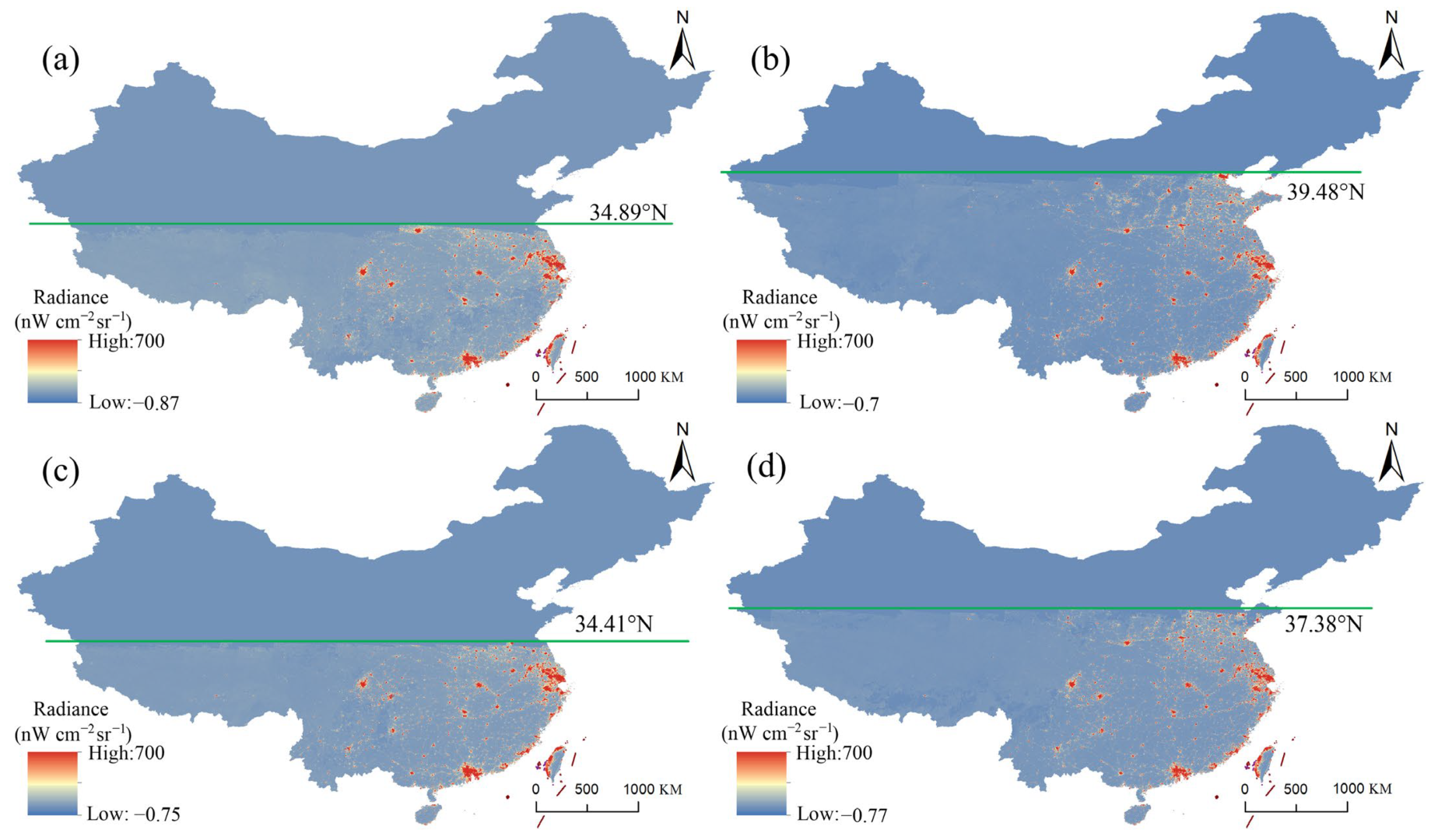
Due to stray light pollution, the pixel values of the Northern Hemisphere summer VIIRS vcm data products are severely lacking, resulting in discontinuities in both time and space in the nighttime light radiation values of the image pixels in this region in their monthly data products (Figure 2); there is a high negative impact on a wide range of studies in various fields based on the long time series VIIRS dataset. Therefore, in this paper, we selected the VIIRS vcm monthly data of Shanghai in 2012–2015, 2018, 2020, and 2021 with complete monthly data of night lights as the research data, choosing the June image data from each year as the data to be interpolated and the six months before and after June as the time-series interpolation data source. The VIIRS vcm data selected for this paper were downloaded from the Earth Observation Group (https://eogdata.mines.edu/products/vnl/) (accessed on 19 June 2022).

Figure 2.
VIIRS vcm images of summer in China. (a) June 2017. (b) July 2017. (c) June 2018. (d) July 2018.
3. Methods
3.1. Research Ideas
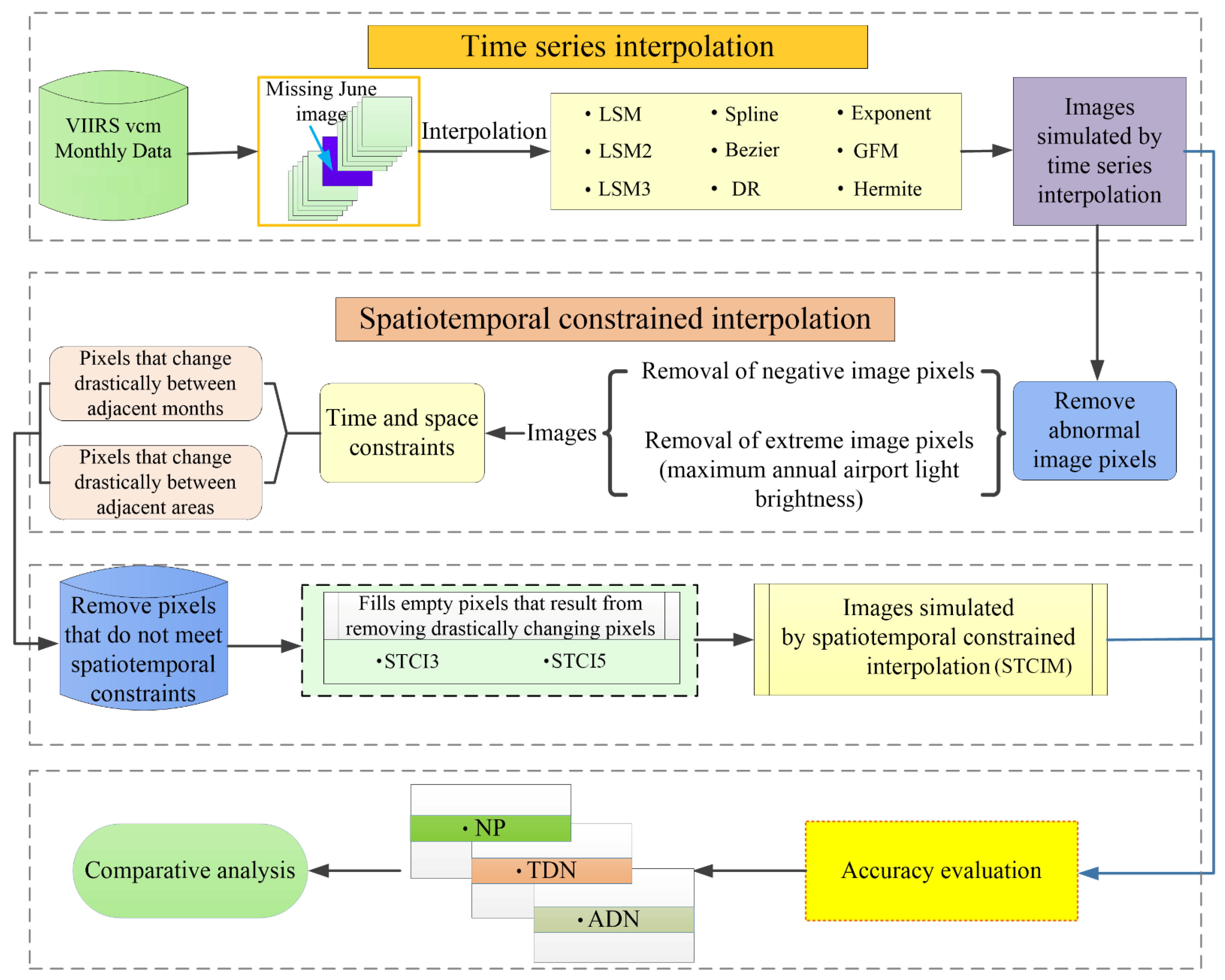
In this paper, we first selected nine widely used time series interpolation methods to interpolate the missing images in June. Second, the abnormal pixels in the interpolated image were removed, including negative value pixels and extremely large abnormal value pixels. At the same time, the pixel-level time continuity constraints and pixel-level spatial correlation constraints of the monthly composite image of VIIRS night lights were constructed. The pixels that did not conform to the constraint relations were identified and eliminated, and the eliminated pixels were filled by using the null pixel focus statistical tool. A monthly composite interpolation dataset with complete spatiotemporal continuity was generated. Finally, we evaluated the accuracy of the nine selected time series interpolation methods and the STCIM. The accuracy evaluation was carried out from the following indicators: NP, TDN, and ADN. The main method flow is shown in Figure 3.

Figure 3.
Flow chart of the method.
3.2. Time Series Interpolation Method
In this paper, we used nine widely used time series interpolation methods, DR, LSM, LSM2, LSM3, Spline, Bezier, GFM, Exponent and Hermite, to perform time series interpolation on the VIIRS DNB vcm data in Shanghai for June of each year. The Hermite interpolation algorithm was implemented in MATLAB R2022a, and other interpolation algorithms were implemented using C++ in the Microsoft Visual Studio 2019 environment.
The DR method is the simplest data assimilation method, where all observations are considered to be accurate, and the observations are directly substituted for the modeled forecast at the corresponding point. In this paper, the missing June nighttime light brightness values for each year were replaced with the average of the image pixel nighttime light brightness values for May and July for each year from 2013–2021, calculated as in Equation (1):
where is the light brightness value of the pixel in the study area in May, is the light brightness value of the pixel in the study area in July, is the simulated light brightness value of the pixel in the study area in June, and is the total number of pixels in the study area.
The LSM method is a mathematical optimization technique whose core purpose is to find the best matching function for the data by minimizing the sum of the squares of errors, estimating certain specific parameters from several available sets of observations to find the unknown data efficiently, and minimizing the sum of squares of errors between the calculated data and the actual data [31]. The LSM was calculated as shown in Equation (2), LSM2 as shown in Equation (3), and LSM3 as shown in Equation (4):
where is the VIIRS vcm month time node, is the light brightness value for the corresponding month time node of the VIIRS, and , , , and are the parameters to be determined.
The Spline method was used to divide an interval into several smaller intervals and interpolate each small interval separately to obtain a continuous and smoothly segmented cubic curve [32], which ensures simple computation, good stability, and easy computer implementation and improves the smoothness of the interpolation function [33]. Suppose there are interpolation nodes on , , and the corresponding light brightness values are . If the function satisfies , on is not higher than the three polynomials. When in has a second-order continuous derivative, is called the Spline.
The Bezier curve method is widely used for parametric curves in numerical analyses. The curve is constructed according to the first and last points of the curve and the control points in the middle [34]. In this study, the lighting data of two adjacent months were used as the start and finish endpoints of the Bezier curve. The lighting data of these two months were combined with the lighting data of their two adjacent months to obtain the control points of the Bezier curve corresponding to the two endpoints. The Bezier curve through the two vertices was drawn according to the endpoints and control points. Since the control points of each Bezier curve segment consisted of endpoints adjacent to the start and finish of the curve, the multi-segment Bezier curve was smooth at the adjacent intersection points. The lighting data for two adjacent months formed a single Bezier curve, and the lighting data for all of the months formed a complete and smooth curve.
The GFM can be used to predict interpolation by fitting the cumulative series of the original data [35]. This method requires less modeling information, is easy to operate, has high modeling accuracy, and can be used to interpolate shorter time series [36], which is suitable for predicting light brightness values for fewer months. When using the GFM, the original data from December 2012–May 2013 were first interpolated in the forward direction. Then, the original data from July–December 2013 were interpolated in the reverse direction. The average value of the two was finally taken as the final interpolated value, and the VIIRS/DNB data in June of each year were interpolated in this manner.
The predicted value obtained by the Exponent method is a weighted sum of the original series, and the closer to the prediction time, the greater the weight [29], which is significantly superior in short- to medium-term predictions [37] and is suitable for the prediction of light brightness values for fewer months. The Exponent will remove the maximum and minimum values from the lighting data for known months and smooth the lighting data. Due to the short length of the original data series, the average of the first three time-series samples was used as the initial value to predict each image pixel of the time series. Similar to the GFM, the Exponent method also uses the forward and inverse interpolation averages as the final interpolation value.
The Hermite interpolation method at a given node requires not only the function value of the interpolation polynomial to be the same as the original function value, but also that at the node, the derivative value of the first order of the interpolating polynomial up to the specified order is equal to the corresponding derivative value of the interpolated function. The curve construction method of Hermite interpolation is the same as that of Spline interpolation, and only the slope values at the endpoints are different. Since the Hermite interpolation curve is conformal [38], even if the original data are not smooth, Hermite interpolation will not overshoot and exceed the numerical range of the original data [39].
3.3. Spatiotemporally Constrained Interpolation Method
3.3.1. Abnormal Pixel Removal
Since the original VIIRS monthly product did not remove transient light sources, such as background noise, firelight, and ship lights, the image of the time series interpolation simulation contained negative pixels and extremely large outlier pixels, collectively referred to as abnormal pixels in this paper. To remove these transient light sources, the negative-valued pixels were reassigned to a value of 0 [40]. Since the airport area has a high light brightness value at night [41], we selected the maximum brightness value of the pixels in the corresponding regions of Shanghai Pudong International Airport (PD) and Shanghai Hongqiao International Airport (HQ) in the original VIIRS vcm month data as the reference value. A reference value was generated each year, and a value greater than the reference value of 10 was used as the threshold value for removing the very large outlier pixels. The thresholds varied from year to year, and the thresholds selected for each year are shown in Table 1.

Table 1.
Maximum value and threshold of light brightness in each year.
3.3.2. Time-Series Nighttime Light Relative Smoothness Feature Constraint
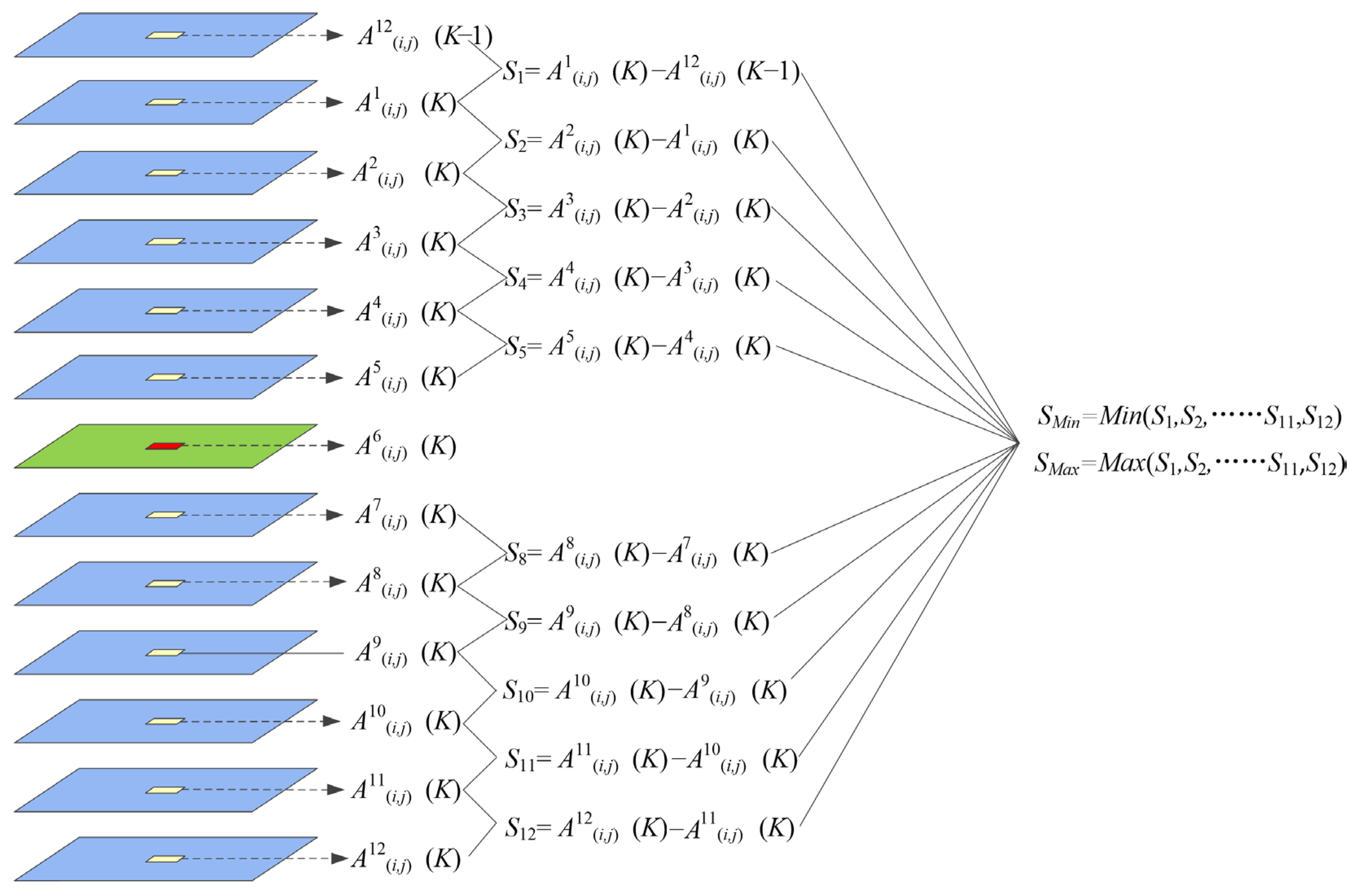
Considering a country or region that has not experienced severe events, such as political turmoil, economic collapse or natural disasters, the light brightness of the region should not change drastically between consecutive months [42]. Let represent the light brightness value of the pixel in row and column of the study area. represents the light brightness value of the pixel in row and column of month , and represents the light brightness value of the pixel in row , column , month , and year . represents the difference between the light brightness value of the pixel in the row and column of the month and the pixel in the row and column of the adjacent month. defines the minimum value of the difference in light brightness of the pixel in row and column in adjacent months of the year, that is, the lower limit value of the difference. represents the maximum value of the difference in light brightness of the pixel in row and column in adjacent months of the year (i.e., the upper limit value of the difference). If the difference in light brightness between the pixel in row and column of the June image simulated by the temporal interpolation method after removing the outliers and the pixel in the corresponding position in the preceding and following months is not within , it is defined as the pixel that changes drastically between months and needs to be eliminated. The extraction process of the pixel that changes drastically between months is shown in Figure 4.
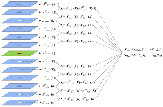
Figure 4.
Calculation chart of the lower and upper limit values for the difference in light brightness between adjacent month pixels.
3.3.3. Constraints on the Relative Stability of the Urban Spatial Structure
Considering the relative stability of the urban spatial structure and the relative stability of the luminous time series of the same objects, the light brightness in adjacent areas should not change drastically [43]. In this study, we calculated the difference in light brightness between the pixel in row , column and the pixels in its neighborhood window of the existing monthly images each year to obtain the minimum and maximum values of the difference between the pixel in row , column and the neighboring pixels for all months in the corresponding year. and , respectively, represent the minimum and maximum values of the difference between the pixel in row and column of month of year and its neighborhood pixels. defines the maximum value of the difference between the pixel in row and column of all months in years and the adjacent pixel, that is, the upper limit of the difference. represents the minimum value of the difference between the pixel in row and column of all months in years and the adjacent pixel, that is, the lower limit of the difference. If the difference between the pixel in row and column of the simulated image in June of the year and the pixels in its neighborhood window is not in , it is defined as the inter-neighborhood variation pixel, which needs to be identified and eliminated. and are calculated as shown in Equation (5) and Equation (6), respectively, and and are computed from Formula (7) and Formula (8), respectively.
3.3.4. Correction of Abnormal Pixels
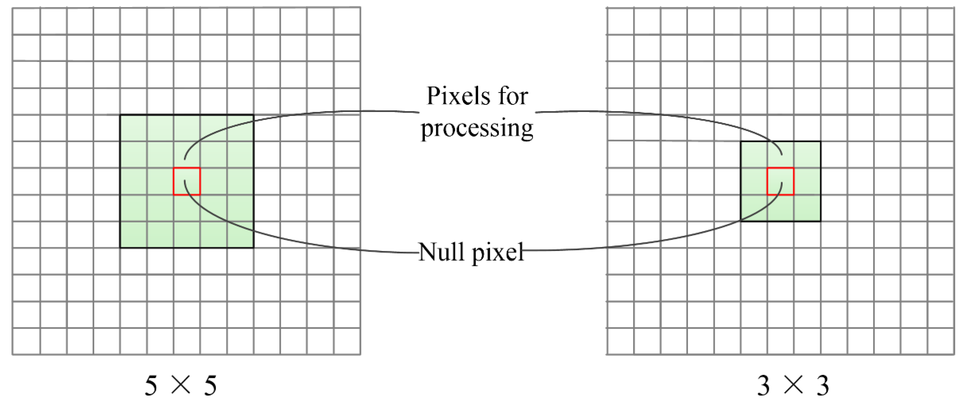
The abnormal pixels, inter-month variation pixels, and inter-neighborhood variation pixels identified in the June image simulated by the time series interpolation method were eliminated. After eliminating pixels, the simulated image had null value pixels that needed to be filled. In this study, considering the relative stability of the urban spatial structure and the relative stability of the luminous time series of the same objects, we used the null pixel focus statistical tool rectangular and neighborhood window of the light brightness of the average value of the image pixel to fill, as shown in Figure 5.
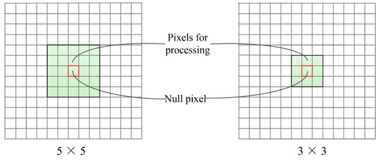
Figure 5.
Null pixel filling map.
3.4. Accuracy Evaluation
In order to evaluate the accuracy of the time series interpolation method and STCIM method, we evaluated the accuracy based on the following indicators: NP, TDN, and ADN.
In this paper, we use NP to represent the number of abnormal pixels in the simulated image, where the abnormal pixels include negative pixels and maximum outlier pixels. The negative pixel refers to the pixel whose light brightness value is negative, and the maximum outlier pixel refers to the pixel whose light brightness value is greater than the annual threshold of light brightness. The maximum thresholds for each year are shown in Table 1; TDN represents the sum of the brightness values of all pixels in the study area; ADN represents the absolute value of the difference in lighting brightness between the simulated image pixel and the corresponding position pixel in the original image.
4. Results
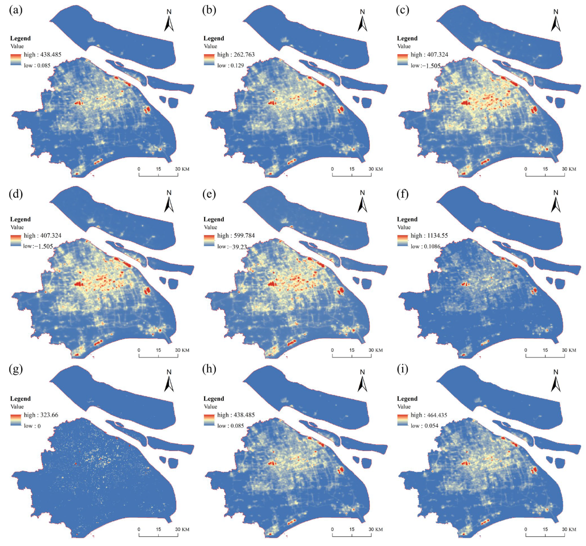
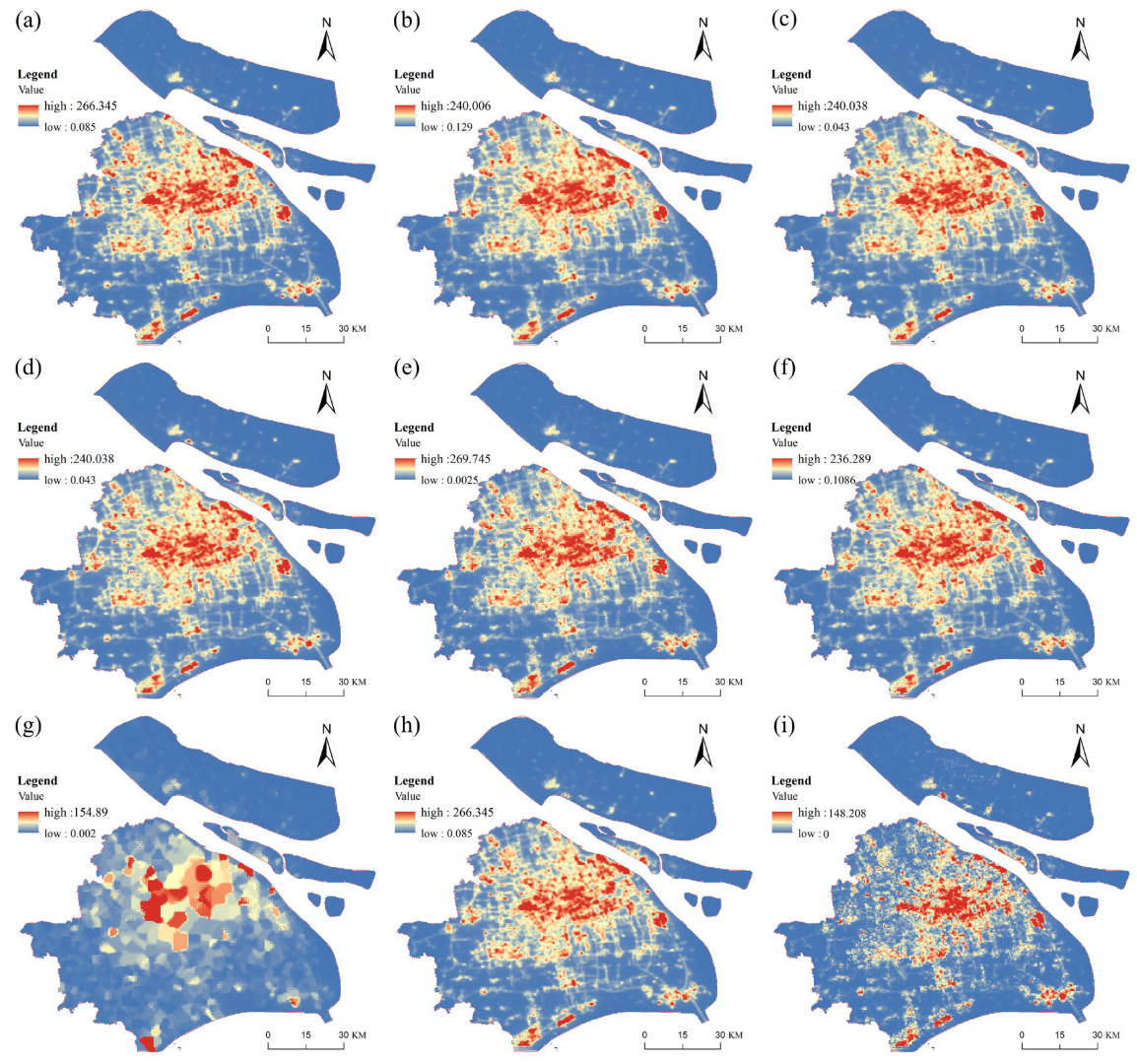
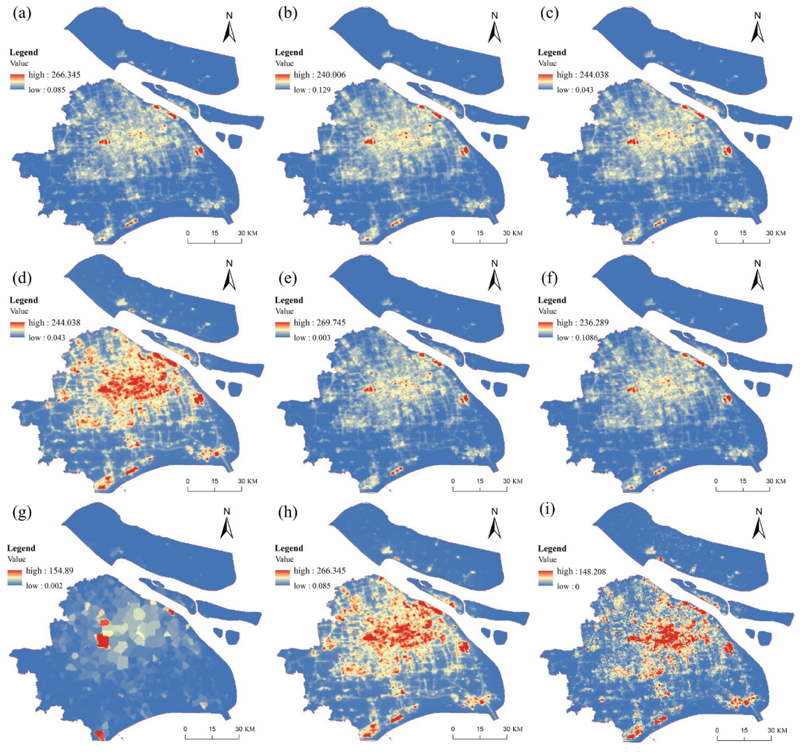
The images of Shanghai in June 2013 that are simulated by the time series interpolation method, spatiotemporally constrained interpolation focus statistics tool rectangular window fill (STCI5), and spatiotemporally constrained interpolation focus statistics tool rectangular window fill (STCI3) are shown in Figure 6, Figure 7 and Figure 8. To verify the accuracy of the time series interpolation method and STCIM in this study, the original VIIRS vcm June image was selected as the reference image. We compared the simulated June image with the original image. The accuracy of time series interpolation and STCIM was evaluated from three aspects: NP, TDN, and ADN.
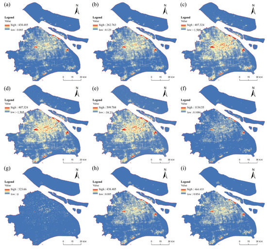
Figure 6.
Image simulated by the time series interpolation method. (a) DR (b) LSM (c) LSM2 (d) LSM3 (e) Spline (f) Bezier (g) GFM (h) Exponent and (i) Hermite.
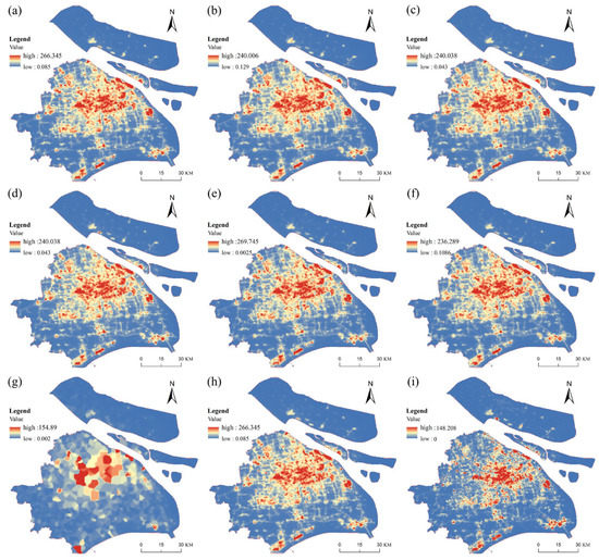
Figure 7.
Image simulated by the spatiotemporally constrained interpolation focuses statistics tool rectangular window fill method. (a) DR (b) LSM (c) LSM2 (d) LSM3 (e) Spline (f) Bezier (g) GFM (h) Exponent and (i) Hermite.
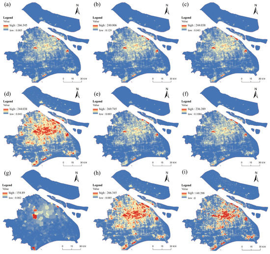
Figure 8.
Image simulated by the spatiotemporally constrained interpolation focuses statistics tool rectangular window fill. (a) DR (b) LSM (c) LSM2 (d) LSM3 (e) Spline (f) Bezier (g) GFM (h) Exponent and (i) Hermite.
4.1. Comparison of the Number of Abnormal Pixels
We calculated the NP in the VIIRS image data simulated by the time series interpolation method, STCI3 method and STCI5 method, including negative pixels and huge anomalous pixels in the images. As shown in Table 2, we found that among the time series interpolation methods, the NP in the images in June of each year simulated by the Spline method was the largest, and the total NP in the June images simulated by the GFM method was the smallest. Moreover, the NP in the images simulated by the DR and Exponent methods in June each year was the same. The NP in the images simulated by the LSM2 and LSM3 methods in June of each year was the same. However, there were no abnormal pixels in the images in June of each year simulated by the STCI3 and STCI5 methods. In terms of NP indicators, the accuracy of the STCIM was higher than that of the time series interpolation method.

Table 2.
The number of abnormal pixels of the interpolated image in June.
4.2. Comparison of Total Light Brightness
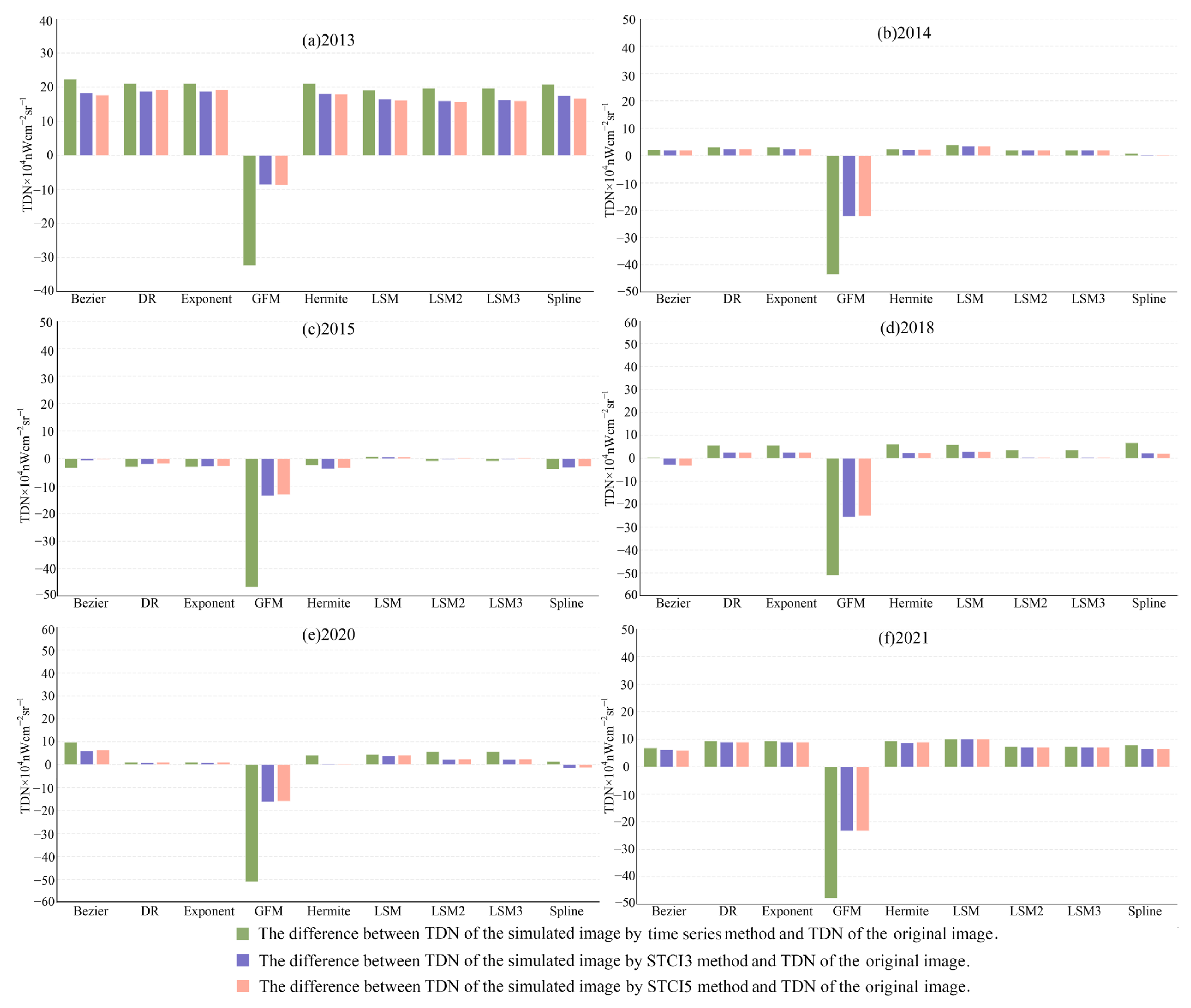
The TDN of the June images simulated by the time series interpolation and STCI3 and STCI5 methods was calculated, and the difference between the TDN of the simulated images and the TDN of the original June image of the corresponding year was calculated. The result is shown in Figure 9, which demonstrates that among the nine methods of time series interpolation used in this study, the GFM method has the worst interpolation effect, and the TDN of the images after GFM interpolation is smaller than the TDN of the original June image of the corresponding year. In 2013 and 2015, the difference between the TDN of the image simulated by the LSM method and the TDN of the original image was the smallest; in 2014, the difference between the TDN of the image simulated by the Spline method and the TDN of the original image was the smallest; in 2018 and 2021, the difference between the TDN of the image simulated by the Bezier method and the TDN of the original image was the smallest; in 2020, the difference between the TDN of the image simulated by the DR and Exponent methods and the TDN of the original image was the smallest, and the time-series interpolation methods applicable to different years were different. The difference between the TDN of the image interpolated by each time series interpolation method in all years and the TDN of the original image was added. The difference between the TDN of the image interpolated by the LSM2 and LSM3 methods and the TDN of the original image was the smallest, and the difference between the TDN of the image interpolated by the GFM method and the TDN of the original image was the largest. We also found that, except for the GFM method, the TDN of the images interpolated by the other methods was higher than that of the original images.

Figure 9.
Difference chart between the TDN of the simulated image and TDN of the original image (TDN of the simulated image—TDN of the original image).
According to the two different focus statistics tools, rectangular window-filling methods of the STCIM, the interpolation results of the two methods are similar. In 2014 and 2020, the effect of the STCI3 method was better than that of the STCI5 method. In 2013, 2015, 2018 and 2021, the effect of the STCI5 method was better than that of the STCI3 method. By adding the difference between the TDN of the interpolated image and the TDN of the original image for each method in all years, we found that the image filled with the STCI5 method was better than the image filled with the STCI3 method. We also found that the difference between the TDN of the image simulated by the time series interpolation method and the TDN of the original image in all years was greater than the difference between the TDN of the image simulated by the STCIM and that of the original image. The TDN of the image simulated by the STCIM method was closer to the TDN of the original image.
4.3. Comparison of Absolute Values of Differences
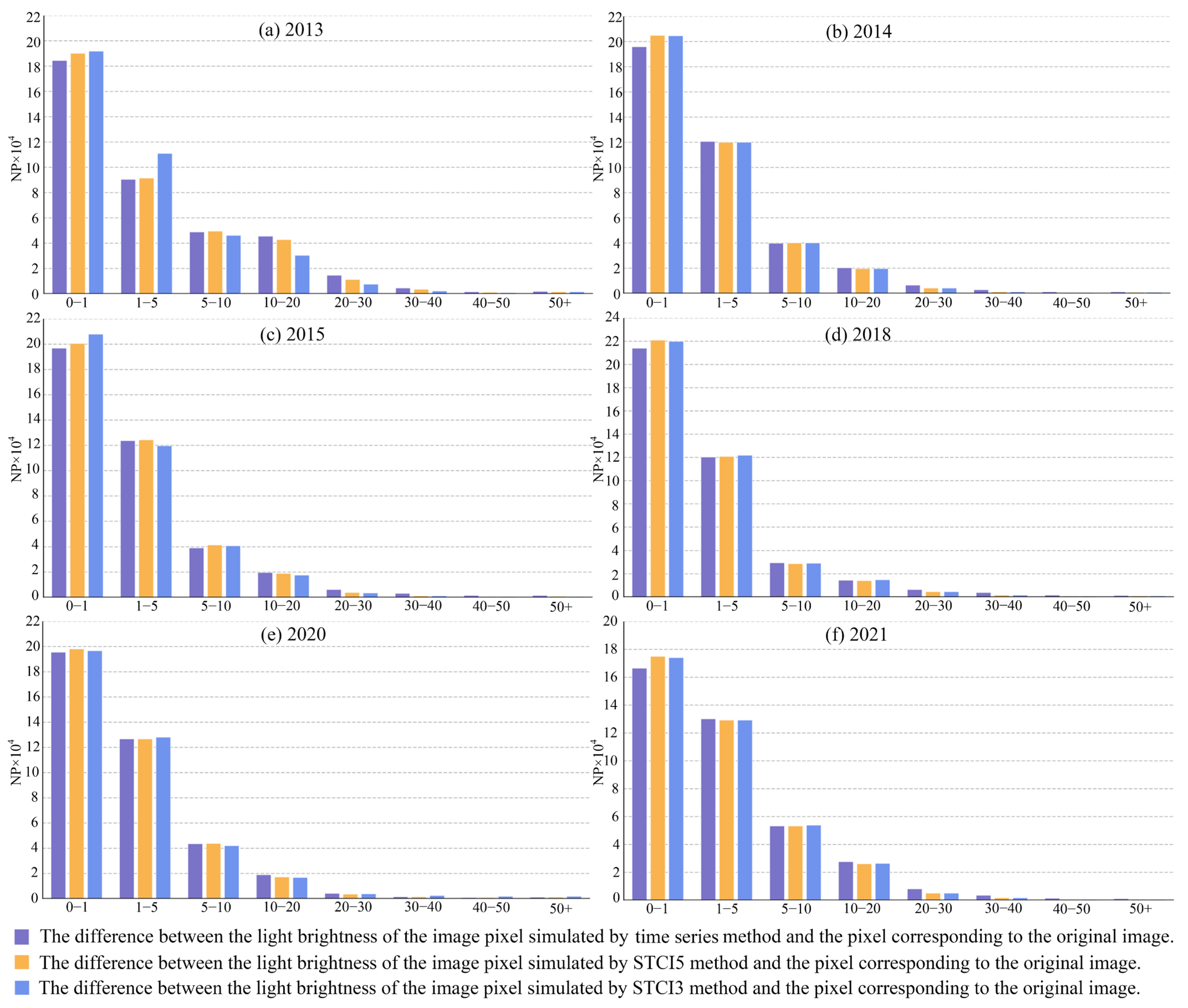
The ADN of the light brightness of the image pixel was simulated by the time series interpolation and STCIM methods, and the light brightness of the corresponding position pixel of the original image was calculated. The calculation was divided into eight grades: 0–1, 1–5, 5–10, 10–20, 20–30, 30–40, 40–50, and greater than 50. Figure 10 shows that the number of pixels with an ADN between 0 and 1 was the largest, and the number of pixels with an ADN greater than 50 was the smallest. The number of pixels with an ADN of 0–5 in the simulated images and original images in each year accounted for more than 80% of the total pixels.
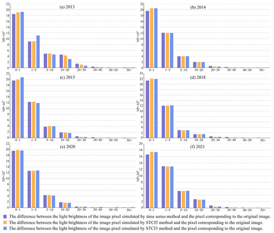
Figure 10.
The number of pixels corresponds to the ADN at different levels.
By comparing the accuracy of images simulated by the time series interpolation and STCIM methods, we found the number of pixels with an ADN of 0–1 between the image simulated by the STCIM method and the original image in all years was higher than the number of pixels with an ADN of 0–1 between the image simulated by the time series interpolation method and the original image. Additionally, the number of pixels with an ADN of 0–5 between the image simulated by the STCIM method and the original image was also higher than the number of pixels with an ADN of 0–5 between the image simulated by the time series interpolation method and the original image. In 2013 and 2015, the number of pixels with an ADN of 0–1 between the image simulated by the STCI3 method and the original image was more than that of the STCI5 and time series interpolation methods. In 2014, 2018, 2020 and 2021, the number of pixels with an ADN of 0–1 between the image simulated by the STCI5 method and the original image was more than that of the ADN of the image simulated by the STCI3 and time series interpolation methods. In the evaluation of the number of pixels whose ADN is located in 0–1, the accuracy of the STCI5 method, STCI3 method and time series interpolation method decreased in turn.
In 2013, 2014 and 2015, the number of pixels with an ADN of 0–5 between the image simulated by the STCI3 method and the original image was more than that of the ADN of the image simulated by the STCI5 and time series interpolation methods. In 2018, 2020 and 2021, the number of pixels with an ADN of 0–5 between the image simulated by the STCI5 method and the original image was more than that of the ADN of the image simulated by the STCI3 and time series interpolation methods. In the evaluation of the number of pixels whose ADN was located in 0–5, the accuracy of the STCI3 method, STCI5 method and time series interpolation method decreased in turn. In conclusion, in terms of ADN, the image accuracy simulated by the STCIM method is higher than that simulated by the time series interpolation method, and the image accuracy simulated by the STCI3 method is higher than that simulated by the STCI5 method.
5. Discussion
Due to stray light pollution, the pixel values of the VIIRS DNB nighttime light data products in the middle and high latitudes of the Northern Hemisphere in the summer are lacking, resulting in a discontinuity in both time and space in the nighttime light radiation values of the pixels in this area in monthly data products. This phenomenon has a very negative impact on research in various fields based on the long-term series VIIRS DNB dataset. To solve this problem, in this study, we propose a spatiotemporally constrained interpolation method that takes into account temporal continuity, relative stability of the urban spatial structure and relative smoothness of nighttime light of the same features in time sequence. By constructing the pixel-level temporal continuity constraint relationship and the pixel-level spatial correlation constraint relationship of the VIIRS DNB night light monthly composite image at the pixel scale, the spatiotemporal constraint interpolation model of the missing image is established, and ultimately, the VIIRS DNB night light monthly composite is realized. The missing pixel value of the image is imputed to generate a monthly synthetic imputation dataset with complete spatiotemporal continuity, and its accuracy was verified.
The spatiotemporally constrained interpolation method proposed in this study simulates images of Shanghai with higher accuracy than the nine temporal interpolation methods used in this paper in terms of NP, TDN and ADN, and the accuracy of image interpolation is significantly improved. The relevant research results are conducive to promoting the application value of nighttime light remote sensing images based on the VIIRS DNB long-term series and enriching the nighttime light remote sensing theory and method system. Furthermore, in the future, we will consider determining the seasonal fluctuation impact factors of pixel values in different types of regions in the time dimension and introduce seasonal fluctuation impact correction parameters into the conventional time series interpolation method. In terms of accuracy evaluation, the socioeconomic indicators of specific sample areas will be considered, and pixel value accuracy analysis and assessment of the imputation result dataset will be carried out. The imputation methods and models will be optimized and improved according to the results of the evaluation.
6. Conclusions
The VIIRS DNB monthly synthetic nighttime light image dataset with complete spatiotemporal continuity is crucial for evaluating human economic activities and urban development. In this study, we propose a spatiotemporally constrained interpolation method for analyzing pixel-level VIIRS monthly products that consider the constraints of temporal continuity and spatial correlation. The accuracy of the time series and spatiotemporally constrained interpolation methods was evaluated from the NP, the TDN, and the ADN. The conclusions of this study are as follows:
- (1)
- Among the nine-time series interpolation methods used, the images simulated by the Spline method had the highest NP, the images simulated by the GFM method had the smallest NP, and the images simulated by the STCI3 method and the STCI5 method had no NP.
- (2)
- The TDN accuracy of the images simulated by the STCIM method was higher than that of the images simulated by the time series interpolation method, and the TDN accuracy of the images simulated by the STCI5 method was higher than that of the images simulated by the STCI3 method.
- (3)
- The number of pixels with an ADN between the light brightness of the image pixel simulated by the STCI5 method and the pixel light brightness of the corresponding position of the original image in the range of 0–1 was the largest. The number of pixels with an ADN between the light brightness of the image pixel simulated by the STCI3 method and the pixel light brightness of the corresponding position of the original image in the range of 0–5 was the largest. The accuracy of the STCIM method was higher than that of the time series interpolation method.
In conclusion, the STCIM method constructed in this paper takes into account the time continuity of VIIRS DNB data, the relative stability of the urban spatial structure, and the relative stability of time series night light for the same objects in the interpolation process, significantly improving the interpolation accuracy. This method also has no strict requirements for timing data before and after the month to be interpolated, making it more widely available. Relevant research results are of great significance to promoting the application of VIIRS DNB night light data and provide data and technical support for research on the urbanization process, spatial estimation of socioeconomic indicators, and assessment of human settlement activity intensity.
Author Contributions
Conceptualization, J.F.; Data curation, Q.L. and J.Z.; Formal analysis, Q.L., J.Z. and P.L.; Funding acquisition, J.F. and Z.R.; Methodology, Q.L., J.F. and Z.R.; Software, Q.L., P.L. and Y.S.; Supervision, J.F.; Visualization, Y.S. and Y.Z.; Writing—original draft, Q.L. and J.F.; Writing—review & editing, J.F. All authors have read and agreed to the published version of the manuscript.
Funding
This work was supported by the National Natural Science Foundation of China (Grant No. 42171413); a grant from the State Key Laboratory of Resources and Environmental Information System; the Shandong Provincial Natural Science Foundation (Grant No. ZR2020MD015 and ZR2020MD018); the National Key Research and Development Program of China (Grant No. 2017YFB0503500); and the Young Teacher Development Support Program of Shandong University of Technology (Grant No. 4072-115016).
Data Availability Statement
The input data used in this research can be accessed freely from online sources.
Acknowledgments
We would like to thank the National Geophysical Data Center of the United States, the Resource and Environmental Science and Data Center Platform, the National Basic Geographic Information Center and the National Geographic Information Public Service Platform for access to the data. We appreciate the editors and reviewers for their constructive comments and suggestions.
Conflicts of Interest
The authors declare no conflict of interest.
References
- Li, X.; Elvidge, C.; Zhou, Y.Y.; Cao, C.Y.; Warner, T. Remote sensing of night-time light. Int. J. Remote Sens. 2017, 38, 5855–5859. [Google Scholar] [CrossRef]
- Elvidge, C.D.; Baugh, K.E.; Kihn, E.A.; Kroehl, H.W.; Davis, E.R.; Davis, C.W. Relation between satellite observed visible-near infrared emissions, population, economic activity and electric power consumption. Int. J. Remote Sens. 1997, 18, 1373–1379. [Google Scholar] [CrossRef]
- Ma, T.; Xu, T.; Huang, L.; Zhou, A. A human settlement composite index (HSCI) derived from nighttime luminosity associated with imperviousness and vegetation indexes. Remote Sens. 2018, 10, 455. [Google Scholar] [CrossRef]
- Lu, D.; Wang, Y.H.; Yang, Q.Y.; Su, K.C.; Zhang, H.Z.; Li, Y.Q. Modeling Spatiotemporal Population Changes by Integrating DMSP-OLS and NPP-VIIRS Nighttime Light Data in Chongqing, China. Remote Sens. 2021, 13, 284. [Google Scholar] [CrossRef]
- Gu, Y.; Shao, Z.F.; Huang, X.; Cai, B.W. GDP Forecasting Model for China’s Provinces Using Nighttime Light Remote Sensing Data. Remote Sens. 2022, 14, 3671. [Google Scholar] [CrossRef]
- Doll, C.N.; Muller, J.P.; Morley, J.G. Mapping regional economic activity from night-time light satellite imagery. Ecol. Econ. 2006, 57, 75–92. [Google Scholar] [CrossRef]
- Chen, X.; Nordhaus, W.D. Using luminosity data as a proxy for economic statistics. Proc. Natl. Acad. Sci. USA 2011, 108, 8589–8594. [Google Scholar] [CrossRef]
- Li, X.; Ge, L.; Chen, X. Detecting Zimbabwe’s decadal economic decline using nighttime light imagery. Remote Sens. 2013, 5, 4551–4570. [Google Scholar] [CrossRef]
- Zhang, Q.; Seto, K.C. Mapping urbanization dynamics at regional and global scales using multi-temporal DMSP/OLS nighttime light data. Remote Sens. Environ. 2015, 115, 2320–2329. [Google Scholar] [CrossRef]
- Xu, T.; Ma, T.; Zhou, C.; Zhou, Y. Characterizing spatio-temporal dynamics of urbanization in China using time series of DMSP/OLS night light data. Remote Sens. 2014, 6, 7708–7731. [Google Scholar] [CrossRef]
- Chen, Z.Q.; Yu, B.L.; Song, W.; Liu, H.X.; Wu, Q.S.; Shi, K.F.; Wu, J.P. A New Approach for Detecting Urban Centers and Their Spatial Structure with Nighttime Light Remote Sensing. IEEE Trans. Geosci. Remote Sens. 2017, 55, 6305–6319. [Google Scholar] [CrossRef]
- Wang, R.; Wan, B.; Guo, Q.H.; Hu, M.S.; Zhou, S.P. Mapping Regional Urban Extent Using NPP-VIIRS DNB and MODIS NDVI Data. Remote Sens. 2017, 9, 862. [Google Scholar] [CrossRef]
- Jiang, L.G.; Liu, Y.; Wu, S.; Yang, C. Study on Urban Spatial Pattern Based on DMSP/OLS and NPP/VIIRS in Democratic People’s Republic of Korea. Remote Sens. 2021, 13, 4879. [Google Scholar] [CrossRef]
- Fan, J.F.; Ma, T.; Zhou, C.H.; Zhou, Y.K.; Xu, T. Comparative Estimation of Urban Development in China’s Cities Using Socioeconomic and DMSP/OLS Night Light Data. Remote Sens. 2014, 6, 7840–7856. [Google Scholar] [CrossRef]
- Fan, J.F.; He, H.X.; Hu, T.Y.; Zhang, P.; Yu, X.; Zhou, Y.K. Estimation of Landscape Pattern Changes in BRICS from 1992 to 2013 Using DMSP-OLS NTL Images. J. Indian Soc. Remote Sens. 2019, 7, 725–735. [Google Scholar] [CrossRef]
- Bagan, H.; Yamagata, Y. Analysis of urban growth and estimating population density using satellite images of nighttime lights and land-use and population data. GISci. Remote Sens. 2015, 52, 765–780. [Google Scholar] [CrossRef]
- Li, X.; Xu, H.M.; Chen, X.L.; Li, C. Potential of NPP-VIIRS nighttime light imagery for modeling the regional economy of China. Remote Sens. 2013, 5, 3057–3081. [Google Scholar] [CrossRef]
- Ma, J.J.; Guo, J.Y.; Ahmad, S.; Li, Z.Q.; Hong, J. Constructing a New Inter-Calibration Method for DMSP-OLS and NPP-VIIRS Nighttime Light. Remote Sens. 2020, 12, 937. [Google Scholar] [CrossRef]
- Li, X.; Zhou, Y.; Zhao, M.; Zhao, X. A harmonized global nighttime light dataset 1992–2018. Sci. Data 2020, 7, 168. [Google Scholar] [CrossRef]
- Yong, Z.W.; Li, K.; Xiong, J.N.; Cheng, W.M.; Wang, Z.G.; Sun, H.Z.; Ye, C.C. Integrating DMSP-OLS and NPP-VIIRS Nighttime Light Data to Evaluate Poverty in Southwestern China. Remote Sens. 2022, 14, 600. [Google Scholar] [CrossRef]
- Jing, X.; Shao, X.; Cao, C.; Fu, X.; Yan, L. Comparison between the Suomi-NPP Day-Night Band and DMSP-OLS for Correlating Socio-Economic Variables at the Provincial Level in China. Remote Sens. 2016, 8, 17. [Google Scholar] [CrossRef]
- Sutton, P.C. A scale-adjusted measure of “urban sprawl” using nighttime satellite imagery. Remote Sens. Environ. 2003, 86, 353–369. [Google Scholar] [CrossRef]
- Elvidge, C.D.; Baugh, K.E.; Anderson, S.J.; Sutton, P.C.; Ghosh, T. The night light development index (NLDI): A spatially explicit measure of human development from satellite data. Soc. Geogr. Discuss. 2012, 7, 23–35. [Google Scholar] [CrossRef]
- Ghosh, T.; Powell, R.L.; Elvidge, C.D.; Baugh, K.E.; Sutton, P.C.; Anderson, S. Shedding light on the global distribution of economic activity. Open Geogr. J. 2010, 3, 148–161. [Google Scholar] [CrossRef]
- Zhao, M.; Cheng, W.M.; Zhou, C.H.; Li, M.C.; Wang, N.; Liu, Q.Y. GDP Spatialization and Economic Differences in South China Based on NPP-VIIRS Nighttime Light Imagery. Remote Sens. 2017, 9, 673. [Google Scholar] [CrossRef]
- Mills, S.; Weiss, S.; Liang, C. VIIRS day/night band (DNB) stray light characterization and correction. In Proceedings of the Earth Observing Systems XVIII, San Diego, CA, USA, 25–29 August 2013; SPIE: Bellingham, WA, USA, 2013; Volume 8866, pp. 549–566. [Google Scholar] [CrossRef]
- Elvidge, C.D.; Zhizhin, M.; Ghosh, T.; Hsu, F.C.; Taneja, J. Annual time series of global VIIRS nighttime lights derived from monthly averages: 2012 to 2019. Remote Sens. 2021, 13, 922. [Google Scholar] [CrossRef]
- Zhao, N.; Hsu, F.C.; Cao, G.; Samson, E.L. Improving accuracy of economic estimations with VIIRS DNB image products. Int. J. Remote Sens. 2017, 38, 5899–5918. [Google Scholar] [CrossRef]
- Chen, M.L.; Cai, H.Y. Interpolation methods comparison of VIIRS/DNB nighttime light monthly composites: A case study of Beijing. Prog. Geogr. 2019, 38, 126–138. [Google Scholar] [CrossRef]
- Fan, J.F.; Zhang, P.; Chen, J.H.; Li, B.; Han, L.S.; Zhou, Y.K. Quantitative Estimation of Missing Value Interpolation Methods for Suomi-NPP VIIRS/DNB Nighttime Light Monthly Composite Images. IEEE Access. 2020, 8, 199266–199288. [Google Scholar] [CrossRef]
- Tian, S.C. The Least Squares Method of Statistical Principles and Applications in Agricultural Pilot Study. Math. Pract. Theory. 2015, 45, 124–133. Available online: https://kns.cnki.net/kcms/detail/detail.aspx?FileName=SSJS201504017&DbName=CJFQ2015 (accessed on 28 June 2022).
- Wang, B.B.; Li, H.J. Temperature Compensation of Piezoresistive Pressure Sensor Based on the Interpolation of Third Order Splines. Chin. J. Sens. Actuators 2015, 28, 1003–1007. [Google Scholar] [CrossRef]
- Li, X. Structure and Matlab Implementation of Cubic Spline Interpolation Endpoint Constraints. J. Shanghai Second. Polytech. Univ. 2012, 29, 319–323. [Google Scholar] [CrossRef]
- Shi, Y.; Jin, D.S. Electrocardiogram pattern recognition method combining bezier curve fitting. Comput. Eng. Des. 2013, 34, 1437–1441. [Google Scholar] [CrossRef]
- Deng, J.L. The main method of the intrinsic grey system. Syst. Eng. Theory Pract. 1986, 6, 60–65. [Google Scholar] [CrossRef]
- He, G. Forecast of regional logistics requirements and application of grey prediction model. J. Beijing Jiaotong Univ. 2008, 7, 33–37. [Google Scholar] [CrossRef]
- Wang, L.; Zhang, Q.; Huang, G.; Tian, J. GPS Satellite Clock Bias Prediction Based on Exponential Smoothing Method. Geomat. Inf. Sci. Wuhan Univ. 2017, 42, 995–1001. [Google Scholar] [CrossRef]
- Han, X. Shape-preserving piecewise rational interpolation with higher order continuity. Appl. Math. Comput. 2018, 337, 1–13. [Google Scholar] [CrossRef]
- Fritsch, F.N.; Carlson, R.E. Monotone piecewise cubic interpolation. SIAM J. Numer. Anal. 1980, 17, 238–246. [Google Scholar] [CrossRef]
- Shi, K.F.; Yu, B.L.; Huang, Y.X.; Hu, Y.J.; Yin, B.; Chen, Z.Q.; Chen, L.J.; Wu, J.P. Evaluating the ability of NPP-VIIRS nighttime light data to estimate the gross domestic product and the electric power consumption of China at multiple scales: A comparison with DMSP-OLS data. Remote Sens. 2014, 6, 1705–1724. [Google Scholar] [CrossRef]
- Ma, T.; Zhou, C.H.; Pei, T.; Haynie, S.; Fan, J.F. Responses of Suomi- NPP VIIRS- derived nighttime lights to socioeconomic activity in China’s cities. Remote Sens. Lett. 2014, 5, 165–174. [Google Scholar] [CrossRef]
- Zhao, N.; Zhou, Y.; Samson, E.L. Correcting Incompatible DN Values and Geometric Errors in Nighttime Lights Time-Series Images. IEEE Trans. Geosci. Remote Sens. 2014, 53, 2039–2049. [Google Scholar] [CrossRef]
- Cheng, G.; Li, Y.L.; Zhao, Z.Z.; Yang, J.; Lu, X.P.; Yuan, D.F. Spatiotemporal Interpolation Methods of NPP/VIIRS Sequence Images Considering Neighbor Relationships. Geomat. Inf. Sci. Wuhan Univ. 2022, 47, 252–260. [Google Scholar] [CrossRef]
Disclaimer/Publisher’s Note: The statements, opinions and data contained in all publications are solely those of the individual author(s) and contributor(s) and not of MDPI and/or the editor(s). MDPI and/or the editor(s) disclaim responsibility for any injury to people or property resulting from any ideas, methods, instructions or products referred to in the content. |
© 2023 by the authors. Licensee MDPI, Basel, Switzerland. This article is an open access article distributed under the terms and conditions of the Creative Commons Attribution (CC BY) license (https://creativecommons.org/licenses/by/4.0/).

