Estimation and Spatiotemporal Analysis of Surface Evaporation in the Yangtze River Basin from 2010 to 2019

Abstract

Evaporation is a critical process involved in energy and water balance at the Earth’s surface and bears significant implications for water resource management, agricultural irrigation, and drought monitoring, among others. In this study, we focused on establishing a 1 km daily surface evaporation estimation for the Yangtze River Basin from 2010 to 2019 by using a machine learning method, and then analyzed its spatiotemporal patterns. The findings showed spatial heterogeneity in the Yangtze River Basin, indicating higher evaporation rates in the southwestern and southeastern regions in contrast to the western and northern areas. Additionally, the basin exhibited a strong spatial autocorrelation, indicating the influence of one spatial unit on the others. Furthermore, most regions in the basin displayed non-significant changes in surface evaporation, with some areas in the upper reaches exhibiting significant increases and a few regions near the source of the Yangtze River experiencing significant decreases. This study contributes to a better understanding of the spatial and temporal distribution of evaporation in the Yangtze River Basin, providing valuable insights for water resource management, environmental studies, and hydrological modeling in the region.

1. Introduction

Evaporation is a crucial variable in global and regional energy and water balance. Understanding its spatiotemporal distribution benefits hydrologic, agricultural, and ecological research and applications [1]. The Yangtze River traverses China from west to east and represents one of the most densely populated and developed regions in the country, encompassing several major cities, including Shanghai, Wuhan and Chongqing. Given the complexity of surface solar radiation, meteorological conditions, and the underlying surface conditions of the Yangtze River Basin, evaporation exhibits substantial temporal and spatial variability. Moreover, the Yangtze River Basin ranks among the most critical water supply areas in China, providing drinking water, irrigation, and industrial water for the population and agriculture within the basin [2]. Therefore, revealing the nature and patterns of evaporation in the Yangtze River Basin is both important and meaningful [3,4,5].

In the current context, research on evaporation within the Yangtze River Basin has primarily relied on data collected from evaporation pans in meteorological stations [6,7]. For instance, Xu et al. [8] estimated reference evapotranspiration and pan evaporation within the Yangtze River Basin. Wang et al. [9] analyzed variations in pan evaporation and reference evapotranspiration across the upper, middle, and lower reaches of the Yangtze River Basin, utilizing daily data from 1961 to 2000 obtained from 115 measuring stations. Rong [10] examined changes in pan evaporation in the upper reaches of the Yangtze River. Ye et al. [2] utilized a modified PenPan model to estimate pan evaporation across the Yangtze River Basin from 1960 to 2019. Their study summarized the spatiotemporal variation patterns and driving factors behind this phenomenon. Given the nonlinearity and complexity of the evaporation process, it is challenging to establish an accurate model that represents all processes and applies to all climatic conditions. If parameters are fixed, the simulation accuracy will vary significantly across different regions. To apply to diverse climatic conditions, empirical estimation methods need to be recalibrated based on the specific climate conditions of their application. Model calibration requires a large amount of data, and the computational cost is high. Providing accurate input values for model calibration also poses challenges, restricting its practical applications in environmental, agricultural, and ecological research.

In recent years, various machine learning techniques have been increasingly employed to estimate surface evaporation within sub-basins of the Yangtze River Basin. For example, Lu et al. [11] employed a range of empirical and machine learning models to estimate daily evaporation in the Poyang Lake Basin for the years 2010–2015. Chen et al. [12] used a support vector machine (SVM) model to estimate monthly pan evaporation for six meteorological stations in the Three Gorges Reservoir area. However, evaporation estimation using machine learning algorithms is usually based on the pan point data of a single observation station, and it only considers the time series characteristics of meteorological elements without effectively considering the spatial correlations of pan evaporation.

Thus, in this study, we focused on the Yangtze River basin and employed machine learning methods, combining observed data from meteorological stations and reanalysis data, to establish a “virtual evaporation pan” network. This network estimated daily 1 km surface evaporation for the Yangtze River Basin from 2010 to 2019 and yielded a high spatiotemporal resolution evaporation dataset. Subsequently, it analyzed the spatiotemporal patterns of evaporation in the Yangtze River basin. This research can enhance our understanding of how evaporation is distributed across time and space within the Yangtze River Basin, offering valuable insights into regional water resource management, environmental research, and hydrological modeling.

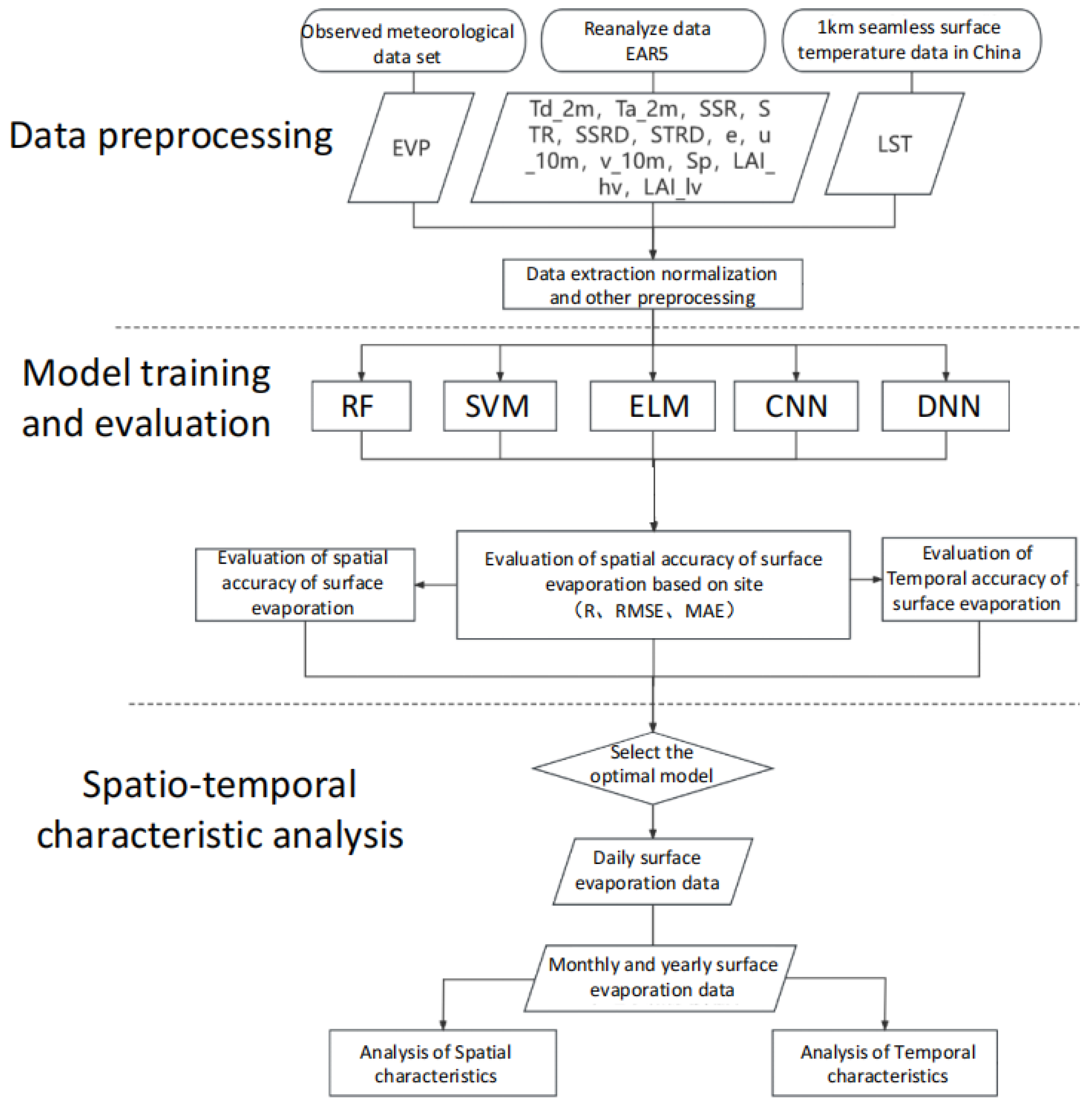
2. Materials and Methods

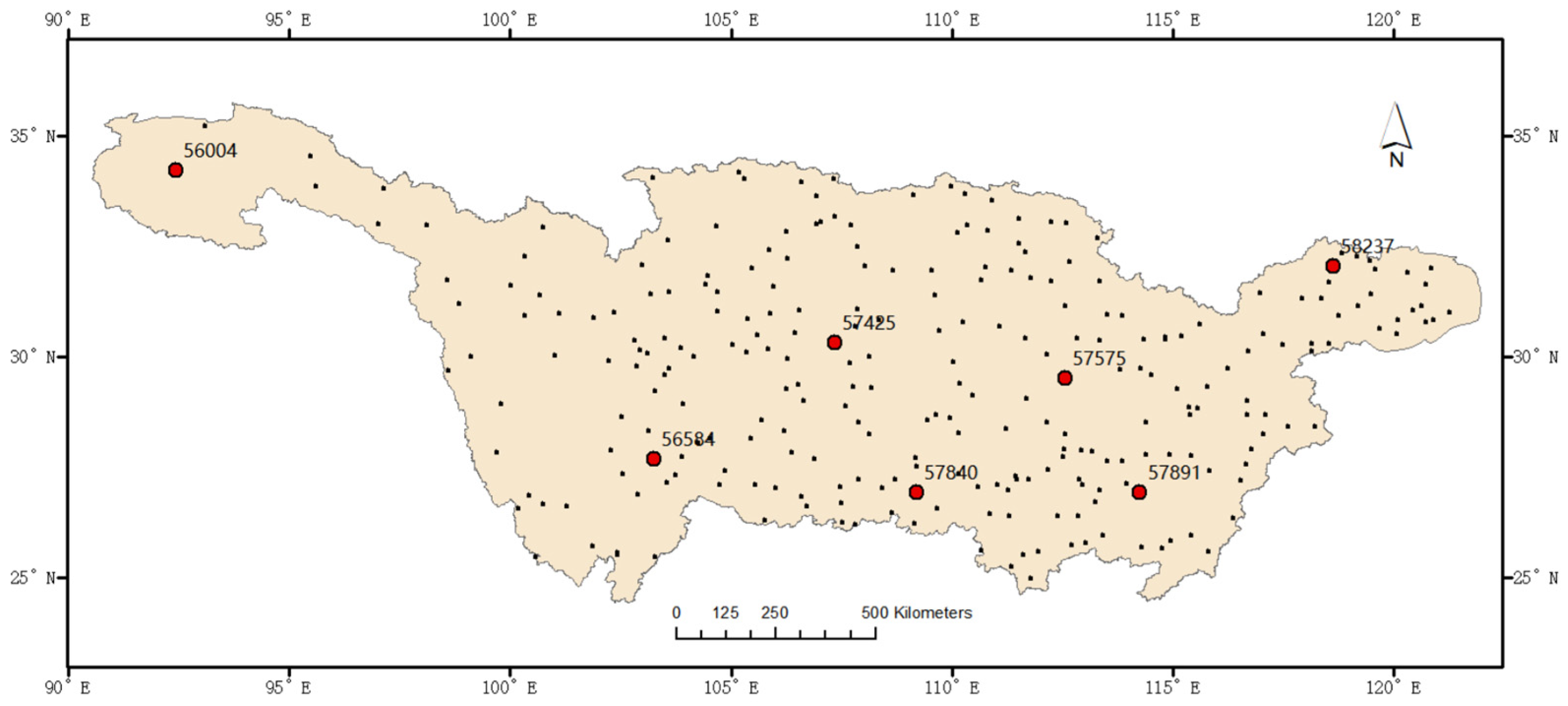
2.1. Study Area and Data

The study area was the Yangtze River Basin. From approximately 24°27′N to 35°54′N latitude and 90°33′E to 122°19′E longitude, this region covers around 1.8 million square kilometers, ranking as the world’s third-largest river basin and occupying 18.8% of China’s land area. It features significant elevation variations, ranging from approximately 5400 m above sea level, and exhibits diverse terrains, topographies, climates, and ecologies. The basin is renowned for its vast size and abundant water resources, contributing about 36% of China’s total river runoff, and it includes major tributaries like the Minjiang River, the Jialing River, and the Hanjiang River. This region experiences a subtropical monsoon climate with notable seasonal variations and influences from monsoons, resulting in natural disasters such as floods and droughts. The diverse climatic environment significantly influences the evaporation process in the Yangtze River Basin, leading to seasonal, regional, and spatial variations. These factors impact the hydrological cycle and the ecosystem within the basin. Various ecological settings within the basin, such as rivers, lakes, forests, and farmlands, also influence the evaporation process. Consequently, evapotranspiration in the Yangtze River Basin is intricately influenced by complex geographical, climatic, and ecological factors.

The data used in this study include the Chinese Ground-Based Climate Data Daily Dataset, the China 1 km Seamless Land Surface Temperature Dataset, and ERA5 reanalysis data. Our meteorological evaporation data for the Yangtze River Basin ranged from 2010 to 2019 and primarily drew from the China Ground-based Climate Data Daily Dataset, which offers two types of evaporation measurements: small (using D20 evaporation pans of 20 cm diameter) and large (using E601B evaporation pans of 62 cm diameter). This study concentrated on small evaporation for practicality and because of data completeness issues related to the large evaporation dataset. In addition, our land surface temperature data were procured from the China 1 km Seamless Land Surface Temperature Dataset, providing 1 km spatial and daily temporal resolutions [13,14,15,16]. This research also harnessed the ERA5 reanalysis dataset by the ECMWF, encompassing meteorological, radiation, surface temperature, and heat flux data with a 0.1° spatial resolution in

Table 1. ERA5 Data information.

For Short	Variable	Implication	Unit
d_2m	2 m dewpoint temperature	2 m dew point temperature	K
t_2m	2 m temperature	2 m air temperature	K
ssr	Surface net solar radiation	Net surface solar radiation	J/m2
str	Surface net thermal radiation	Net surface heat radiation	J/m2
ssrd	Surface solar radiation downwards	Solar radiation descending from the surface	J/m2
strd	Surface thermal radiation downwards	Descending surface heat radiation	J/m2
e	Total evaporation	Total evaporation	m/d
u_10m	10 m u-component of wind	Wind speed in the U direction at 10 m	m/s
v_10m	10 m v-component of wind	Wind speed in the V direction at 10 m	m/s
sp	Surface pressure	Surface pressure	Pa
lai_hv	Leaf area index, high vegetation	High vegetation leaf area index	/
lai_lv	Leaf area index, low vegetation	Low vegetation leaf area index	/

. It is important to note that the meteorological data underwent a transformation; we averaged hourly data into daily values, and the radiation data involved summarizing 12 h values to yield daily averages. A comprehensive overview of the variables necessary for building machine learning models, along with their corresponding data product details, is outlined in

Table 2. Model builds data product.

Data Type	Product	Variable	Spatial Resolution	Time Resolution	Data Source
Measured data	Daily value data set of surface climatological data for China	Evaporation (EVP) measured in small evaporating dish (E20)	/	1 day	National Meteorological Science Data Center
Reanalysis data	ERA5	d_2m, t_2m, ssr, str, ssrd, strd, e, u_10m, v_10m, sp, lai_hv, lai_lv	0.1°	1 h	https://cds.climate.copernicus.eu/cdsapp#!/dataset/reanalysis-era5-land?tab=overview (accessed on 10 November 2022)
Other data	China region 1 km seamless surface temperature dataset (2002–2020)	LST	1 km	1 day	National Tibetan Plateau Data Center

.

2.2. Estimation of Surface Evaporation in the Yangtze River Basin within Machine Learning

This research is divided into three main parts, as shown in Figure 1: data preprocessing; model training and evaluation; and spatiotemporal feature analysis. Initially, ERA5 reanalysis data, recorded meteorological data, and surface temperature data underwent data extraction and normalization as part of the preprocessing. Subsequently, five distinct machine learning algorithms were employed for model training, followed by site-specific spatial accuracy assessments and time series analyses. The machine learning model demonstrating the highest performance was selected to produce daily 1 km surface evaporation datasets for the Yangtze River Basin spanning the years 2010 to 2019. These datasets were then utilized to derive monthly, annual, and decadal evaporation data, allowing for a comprehensive investigation of the associated spatiotemporal features.

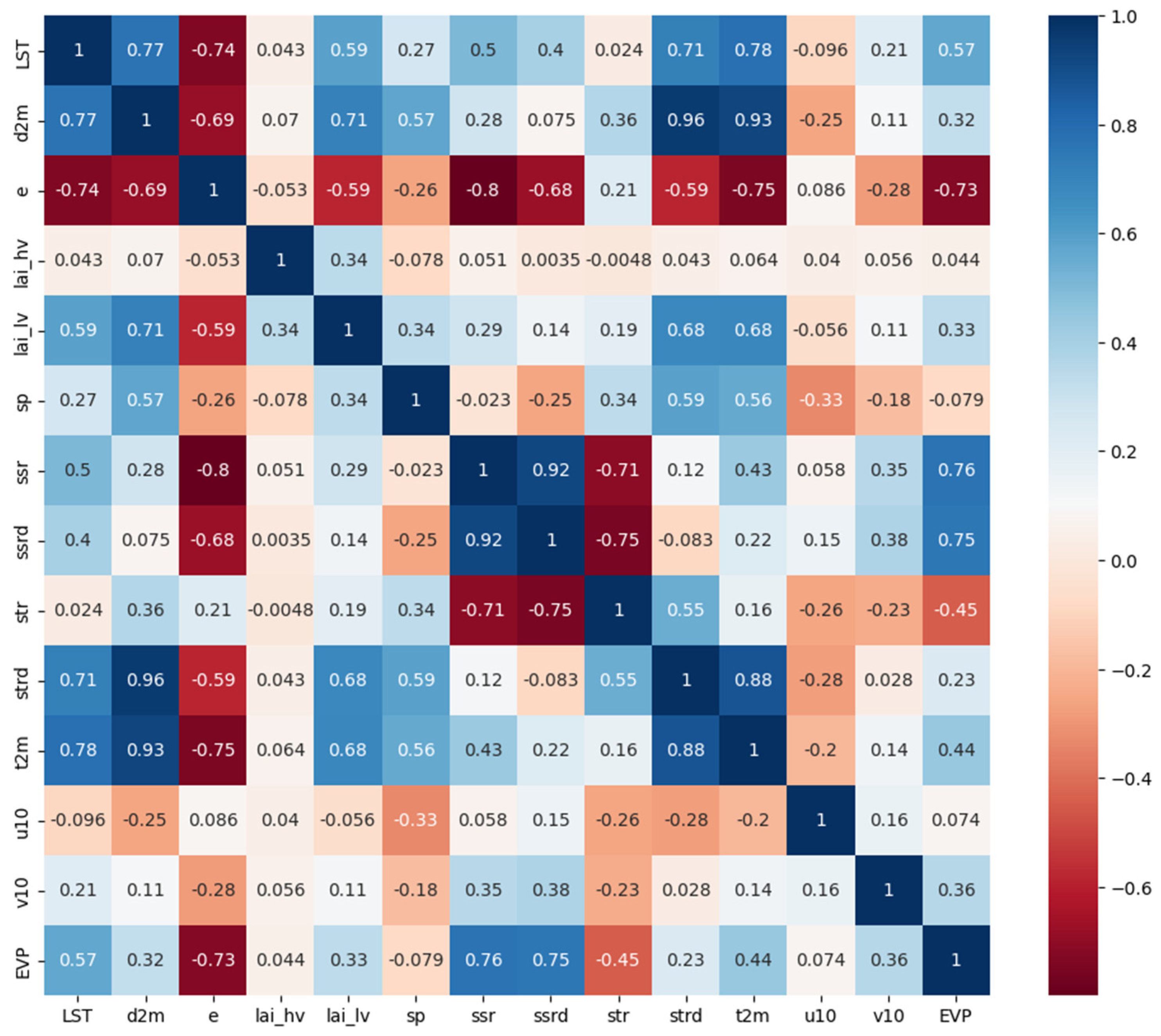
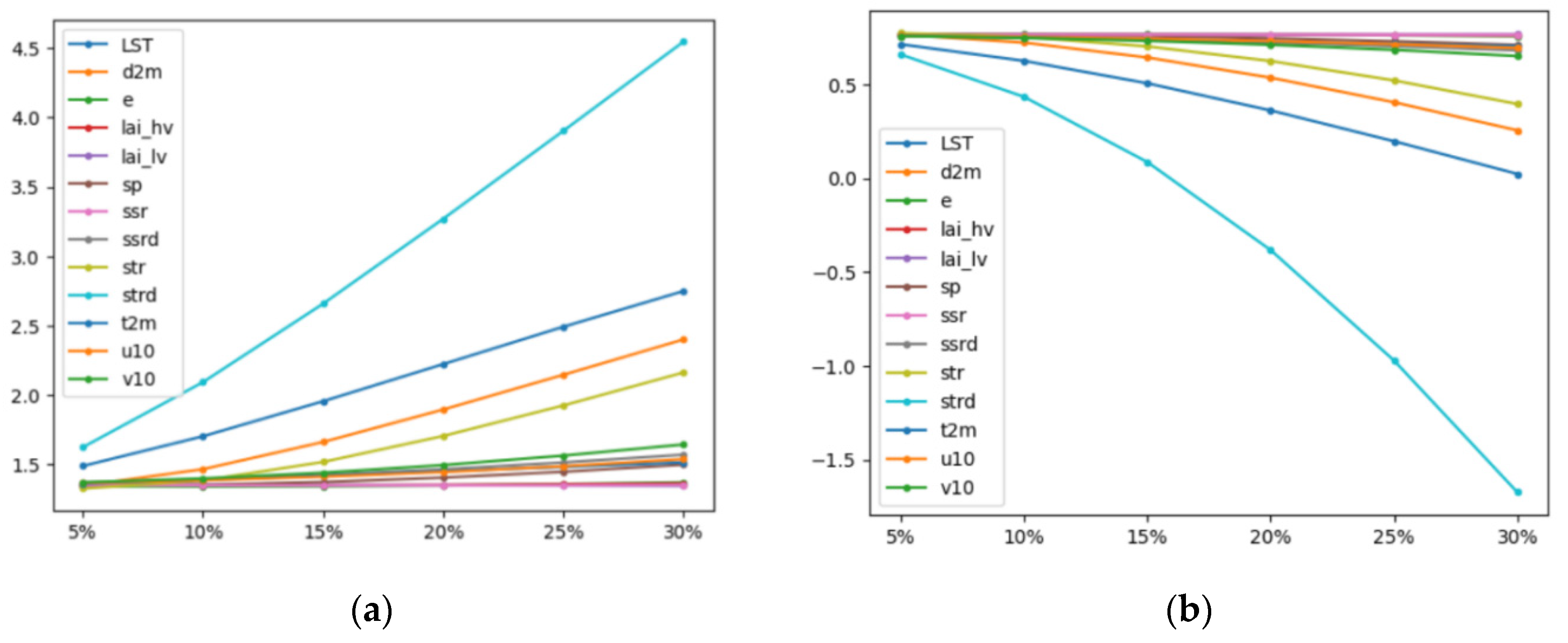
2.2.1. Variable Selection

Based on previous evaporation simulation studies and the availability of meteorological data, for this study, we selected a set of 13 input variables, as illustrated in

Table 3. Model variable statistics.

Variable Name	Variable Meaning	Minimum	25% Value	50% Value	75% Value	Maximum	Mean	Standard Deviation
LST	Surface temperature (K)	270.1144	290.8603	297.7726	305.3267	344.592	298.1359	9.833419
d2m	2 m dew point temperature (K)	234.5368	273.9738	282.3932	290.1296	301.3116	281.0068	11.45174
e	Total evaporation (m/d)	−0.00582	−0.00247	−0.00131	−0.00066	3.19 × 10−5	−0.00163	0.001187
lai_hv	High vegetation leaf area index	−4.44 × 10−16	0.930162	2.160215	2.497014	5.878531	1.942995	1.250639
lai_lv	Low vegetation leaf area index	0.165024	1.25906	1.731728	2.336332	3.566517	1.802465	0.680875
sp	Surface pressure (Pa)	55,729.63	86,067.28	93,759.58	98,021.01	103,896.8	89,369.74	12,341.6
ssr	Surface Net Solar Radiation (J/m2)	436,639.9	4,867,988	8,848,731	12,848,888	21,770,216	8,990,494	4,729,407
ssrd	Surface Net Solar Radiation (J/m2)	490,030.3	6,515,555	11,113,285	15,512,798	26,533,810	11,105,916	5,583,336
str	Surface Net Heat Radiation (J/m2)	−8,013,409	−3,582,834	−2,407,841	−1,420,580	275,050.2	−2,551,303	1,384,084
strd	Surface Net Heat Radiation (J/m2)	4,556,421	13,004,630	15,291,245	17,438,143	21,136,594	14,965,575	3,137,576
t2m	2 m air temperature (K)	249.2020	278.6251	286.8802	294.3579	309.7132	285.7649	11.46349
u10	10 m meridional wind speed (m/s)	−9.45987	−0.82943	−0.2765	0.256194	9.524438	−0.27517	0.997803
v10	10 m zonal wind speed (m/s)	−8.60936	−0.83048	−0.06951	0.597828	7.586802	−0.09855	1.378779

. The output variable chosen for the model was as-measured pan-evaporation data (EVP).

The total evaporation data ‘e’ extracted from the ERA5 dataset are represented by negative values, signifying evaporation, and positive values, indicating condensation, and it exhibits substantial fluctuations. A similar level of volatility is observed in the high vegetation index. When examining the minimum and 25% values of surface pressure, it becomes evident that the majority of sites are situated at lower elevations.

Pearson correlation coefficients were computed for the 14 meteorological and radiation variables, and the findings are presented in Figure 2. The figure illustrates that the two variables exhibiting the highest correlation are ‘d2m’ and ‘strd’, with a correlation coefficient of 0.96, suggesting an almost linear correlation. Similarly, strong correlations are observed between ‘d2m’ and ‘t2m’ as well as ‘ssrd’ and ‘ssr’, both exceeding 0.9.

Ranking the variables according to their degree of correlation with the measured pan evaporation data ‘EVP’, we find the sequence from the most to the least correlated as follows: ‘ssr’, ‘ssrd’, ‘e’, ‘LST’, ‘str’, ‘t2m’, ‘v10’, ‘lai_lv’, ‘d2m’, ‘strd’, ‘sp’, ‘u10’, ‘lai_hv.’ Notably, ‘ssr’, ‘ssrd’, and ‘e’ display strong correlations, ‘LST’, ‘str’, and ‘t2m’ exhibit moderate correlations, while ‘v10’, ‘lai_lv’, ‘d2m’, and ‘strd’ show weaker correlations. On the other hand, ‘sp’, ‘u10’, and ‘lai_hv’ demonstrate weak or negligible correlations.

Among the input variables exhibiting weaker correlations, ‘dew point temperature’ is primarily linked to relative humidity, a factor closely tied to evaporation based on prior experience. Additionally, the combination of ‘u10’ and ‘v10’ can be used to calculate the wind speed at 10 m, a significant factor influencing evaporation. The ‘lai’ index reflects the extent of vegetation cover, directly impacting the specific surface emissivity, which subsequently affects the surface’s upward long-wave radiation. The disparity between downgoing and upgoing long-wave radiation determines the net surface heat radiation.

2.2.2. Machine Learning Model

• Random Forest

The random forest (RF) algorithm [17,18] was developed by Leo Breiman at the turn of the century; it is a decision-tree-based machine learning method that has been used extensively for predicting land surface parameters in recent years.

Within this study, the model’s output comprises the measured evaporation derived from meteorological station data. The model incorporates 13 input variables (xp), encompassing surface temperature (LST), dew point temperature at a 2 m height (d2m), total evaporation values (e) obtained from ERA5, the high-vegetation leaf area index (lai_hv), the low-vegetation leaf area index (lai_lv), surface air pressure (sp), surface net solar radiation (ssr), surface-descending solar radiation (ssrd), surface net thermal radiation (str), surface downlink thermal radiation (strd), temperature at 2 m (t2m), U-direction wind speed at 10 m (u10), and V-direction wind speed at 10 m (v10). These variables were analyzed across a total of 234 sites, resulting in a dataset comprising 355,144 measured evaporation data points, denoted as “n = 355,144” samples.

2.

Support Vector Machines

The support vector machine (SVM) algorithm [19] was introduced by Cortes and Vapnik in 1995 for binary data classification, and it has since evolved to address both linear and nonlinear problems.

We used 13 key indicators as inputs for this model. The measured evaporation serves as the model’s output. The SVM model was trained and constructed with a cache size set at 7000; the decision function type “ovr”, denoting one-to-many; and a training stopping threshold of 1 × 10⁻³.

3.

Extreme Learning Machine

The extreme learning machine (ELM) [20,21] is a single-hidden-layer feedforward neural network originally introduced by Professor Huang Guangbin in 2004, serving as a learning algorithm for such networks.

In the context of this study, the model’s input layer (xi) comprises 13 feature vectors, including the variables LST, ssrd, str, and strd. The output layer corresponds to the measured evaporation in the pan (σj). Specifically, the number of hidden layer nodes is set to L = 64. This involves obtaining generalized inverse and transpose matrices, followed by calculating the output weight matrix through matrix multiplication. The parameter values are saved, along with the neural network itself. The model’s iterations are set to 2000. Subsequently, using the saved model training parameters, we can calculate the prediction results for evaporation concentration, verifying the model’s predictive performance.

4.

Deep-Learning Neural Network

The deep-learning neural network (DNN) was originally based on the multi-layer perceptron (MLP) introduced in 1965; an enhanced DNN [22] is capable of acquiring more sophisticated and abstract high-level features compared with shallow neural networks.

In the context of this evaporation simulation experiment, the model is structured with three hidden layers. The input layer is composed of 13 variables, including LST and ssr. This process involves forward execution to transform the input layer, yielding layer 1. This process is executed twice to produce layer 2 and layer 3. The final result, layer 4, represents the output variable of the model, which corresponds to the measured evaporation data from the evaporation pan. The model parameters are defined as follows: there are 2000 epochs; the number of iterations is set to 2000; and there are 64, 128, and 64 hidden layer nodes in the three respective hidden layers with a single output variable.

5.

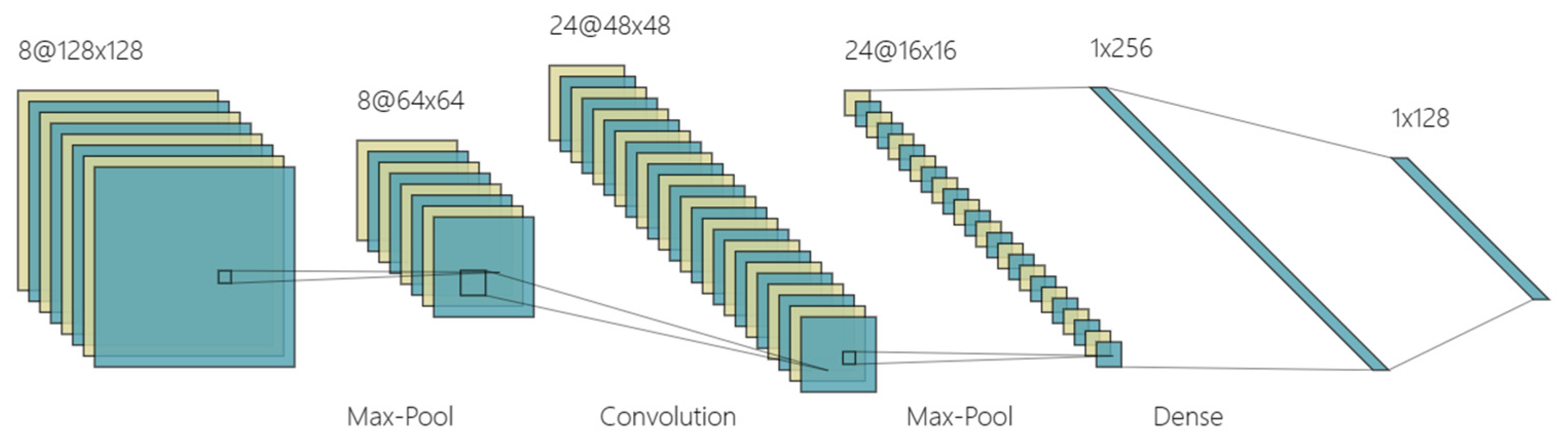
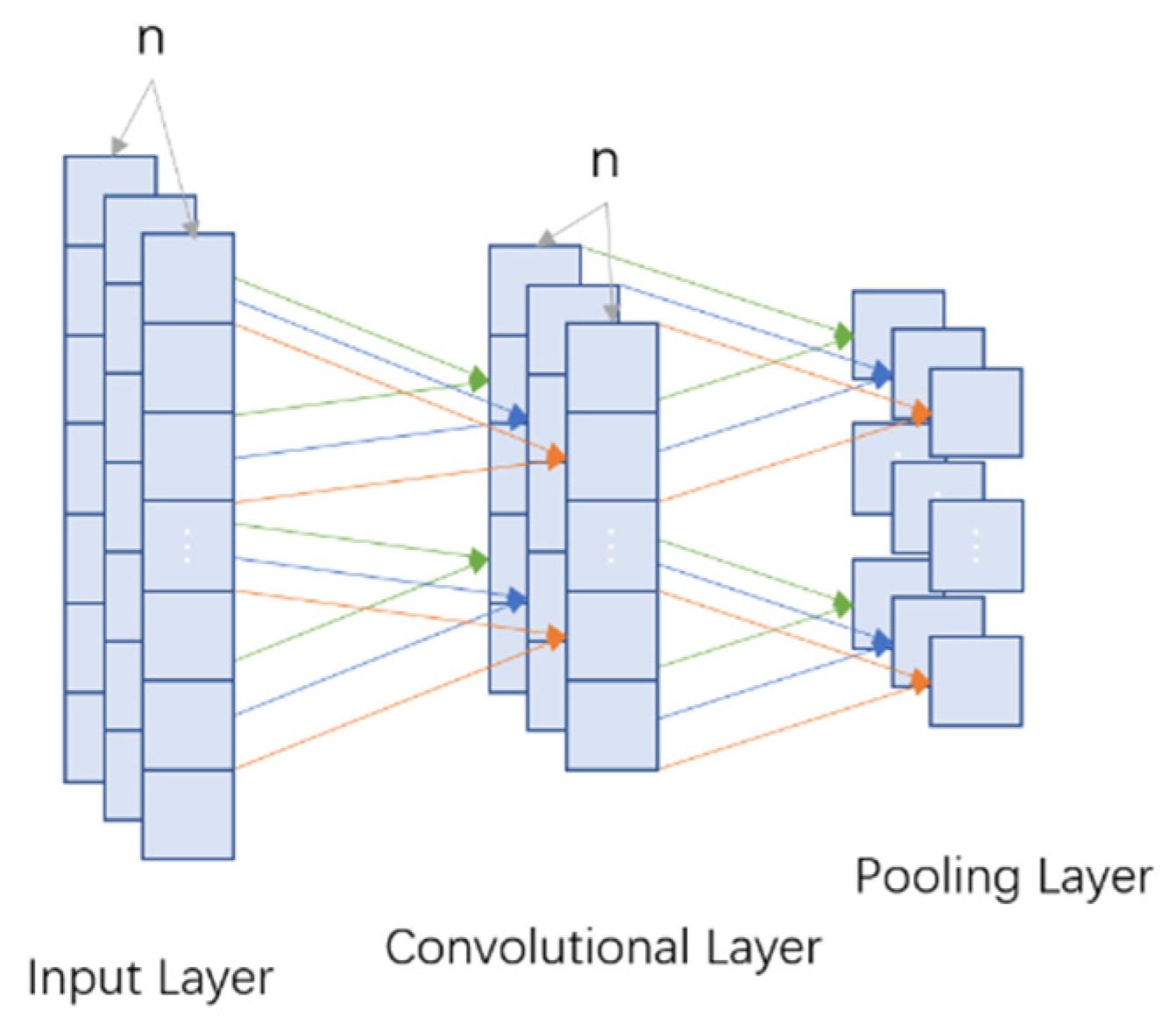
Convolutional Neural Network

The convolutional neural network (CNN) [23] generally has three main types of layers in Figure 3: convolutional layers, pooling layers, and fully connected (FC) layers.

In this study, 1-dimensional meteorological data characteristics, namely 1-dimensional vectors, were used as the CNN’s input. Therefore, the convolutional kernel and the feature graph inside the network are also 1-dimensional [24]. In each CNN layer, 1-dimensional forward propagation (1D-FP) is represented as follows:

$${\mathrm{x}}_{\mathrm{k}}^{\mathrm{l}}={\mathrm{b}}_{\mathrm{k}}^{\mathrm{l}}+\sum _{\mathrm{i}=1}^{{\mathrm{N}}_{\mathrm{l}-1}}\mathrm{c}\mathrm{o}\mathrm{n}\mathrm{v}1\mathrm{D}({\mathrm{w}}_{\mathrm{i}\mathrm{k}}^{\mathrm{l}-1},{\mathrm{s}}_{\mathrm{i}}^{\mathrm{l}-1})$$

(1)

where ${\mathrm{x}}_{\mathrm{k}}^{\mathrm{l}}$ is defined as the input, ${\mathrm{b}}_{\mathrm{k}}^{\mathrm{l}}$ is limited to the bias of the k-th neuron in layer l, ${\mathrm{s}}_{\mathrm{i}}^{\mathrm{l}-1}$ is the output of the i-th neuron in layer l − 1, and ${\mathrm{w}}_{\mathrm{i}\mathrm{k}}^{\mathrm{l}-1}$ from the i-th neuron in layer l − 1 to the k-th neuron in layer l. $\mathrm{c}\mathrm{o}\mathrm{n}\mathrm{v}1\mathrm{D}\left(\right)$ is used to perform a valid 1-dimensional convolution without zero padding. Therefore, the dimension of the input array, ${\mathrm{x}}_{\mathrm{k}}^{\mathrm{l}}$, is less than the dimension of the output array, ${\mathrm{s}}_{\mathrm{i}}^{\mathrm{l}-1}$.

Figure 4 shows the structures of the convolution layer and the pooling layer when a 1-dimensional CNN network is used to simulate evaporation with meteorological data. In the CNN’s input, meteorological variables extracted from each meteorological dataset are used to form the feature vector of the CNN’s input. The 1-D CNN network used in this study uses 2 × 1 and 3 × 1 convolution kernels. Given that the dimension of the eigenvector is small, the convolution kernel here is correspondingly small. In this study, a maximum pooling layer was adopted. The final fully connected layer uses a two-layer structure, and the final output is a single value; that is, the final fully connected layer realizes the regression function.

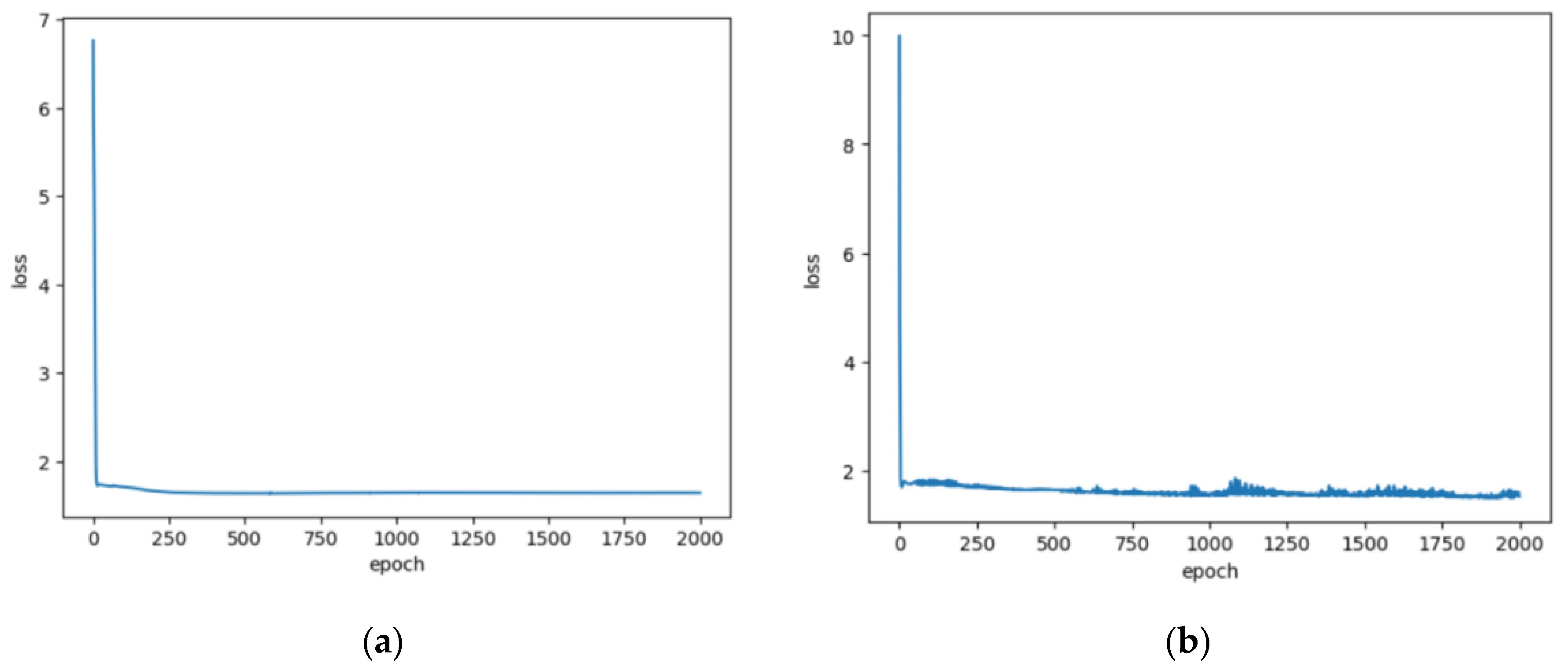
2.2.3. Model Training

In this chapter, data spanning the years 2010 to 2019 from 234 meteorological observation stations within the Yangtze River Basin were assimilated, incorporating ERA5 data and surface temperature data. Five distinct machine learning algorithms—RF, SVM, ELM, CNN, and DNN—were harnessed to estimate surface evaporation, focusing on station-based estimations.

For each machine learning algorithm, the dataset was divided into a training set (comprising 70% of the data) and a test set (encompassing the remaining 30%), with random selection. To assess the spatial accuracy, the test data from all stations were utilized, while the data from 7 meteorological stations specifically served to evaluate spatial accuracy.

Detailed descriptions of the training outcomes for each of the five models will be elaborated in Section 3.1.

It is crucial to standardize all input and output variables before commencing model training. Failure to do so can result in a considerably slow gradient descent process, leading to inefficient resource utilization and reduced processing efficiency. The MinMaxScaler normalization function was employed for this standardization, implemented as follows:

$$X_{\mathrm{std}}=\frac{X_{\mathrm{i}}-X_{\min }}{X_{\max }-X_{\min }}$$

(2)

X_std is the standardized value, calculated as X_min represents the minimum sample value, and X_max represents the maximum sample value. X_std falls within the range of 0 to 1, with a total of 355,144 samples.

2.2.4. Methods for Spatial Analysis of Surface Evaporation

In this study, the spatial analysis of surface evaporation in the Yangtze River Basin encompasses the following aspects:

• Analysis of the spatial distribution characteristics of evaporation in the Yangtze River Basin based on ten-year average evaporation data and annual evaporation data.
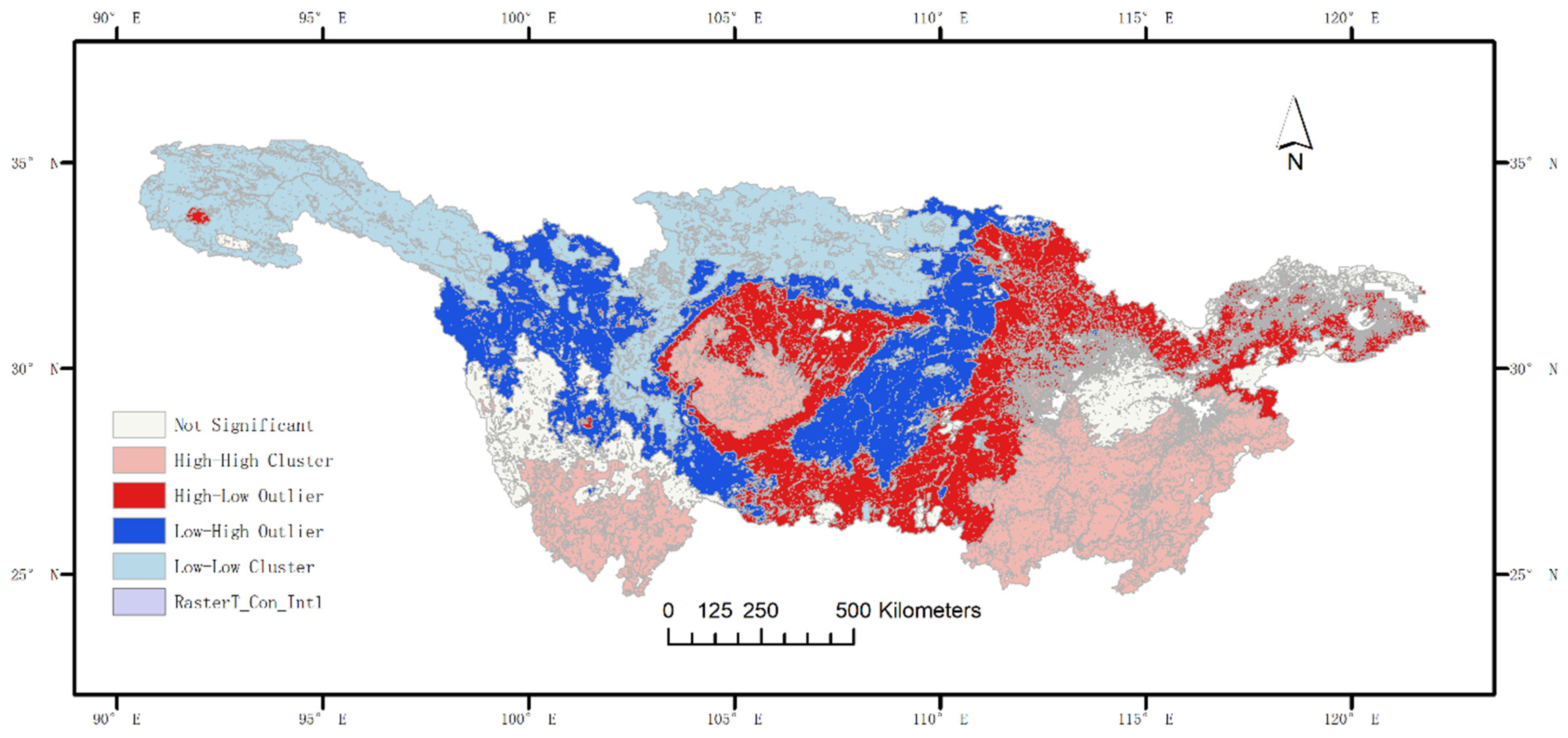
• Conducting spatial autocorrelation analysis by calculating global and local Moran indices to determine the presence of spatial autocorrelation and identify clustering types and regions.

Spatial autocorrelation statistics are employed to reveal correlations within variables, whereas spatial autocorrelation investigates correlations across different spatial locations for the same variable. To investigate whether a correlation exists between surface evaporation at a specific spatial location and its neighboring spatial locations, as well as to determine the extent of this correlation, spatial autocorrelation statistics are applied to evaporation data. Initially, global autocorrelation analysis is conducted to determine whether the distribution of evaporation is random or clustered throughout the entire Yangtze River Basin. If clustering is observed, local autocorrelation analysis is subsequently performed to identify areas and types of aggregation.

The Moran index is a commonly used method for spatial autocorrelation analysis, and it is divided into Global Moran’s I index and Local Moran’s I index. The former, introduced by Moran in 1948, quantifies the degree of similarity among attribute values of spatially adjacent or neighboring regional units.

$$I_{Global}=\frac{n{\displaystyle \sum _{i=1}^n{\displaystyle \sum _{j=1}^n{\omega }_{ij}(E_{\mathrm{p}}{}_i-\overline{E_{\mathrm{p}}})(E_{\mathrm{p}}{}_j-\overline{E_{\mathrm{p}}})}}}{({\displaystyle \sum _{i=1}^n{\displaystyle \sum _{j=1}^n{\omega }_{ij}}}){\displaystyle \sum _{i=1}^n{(E_{\mathrm{p}}{}_i-\overline{E_{\mathrm{p}}})}^2}}$$

(3)

where n represents the number of spatial elements, that is, the number of grids in the Yangtze River Basin; E_pi and E_pj in the i and j tent of evaporation attribute value, respectively; $\overline{E_{\mathrm{p}}}$ represents the average evaporation of all space cells; ${\omega }_{ij}$ represents the first (i, j) element of the spatial weight matrix, which is essentially a kind of artificial spatial proximity relationship, reflecting the spatial relationship between the cell and other cells.

The value of Global Moran’s I ranges from [−1, 1]. The greater the absolute value of Global Moran’s I, the stronger the spatial correlation of evaporation. The closer the absolute value is to zero, it means that the evaporation is distributed randomly in space, that is, there is no spatial correlation. When Global Moran’s I > 0, indicating a positive spatial correlation, attributes of the same evaporation amount cluster together. The larger the absolute value is, the smaller the difference between spatial units is. When Global Moran’s I < 0, indicating spatial negative correlation, different properties of evaporation are clustered together. The greater the absolute value, the greater the difference between spatial units.

The calculated Moran index is tested for Z-distribution significance:

$$Z_{I_{G\mathrm{lobal}}}=\frac{I_{G\mathrm{lobal}}-E(I_{G\mathrm{lobal}})}{\sqrt{VAR(I_{G\mathrm{lobal}})}}$$

(4)

$$E(I_{G\mathrm{lobal}})=-\frac{1}{n-1}$$

(5)

$$VAR(I_{G\mathrm{lobal}})=E(I_{G\mathrm{lobal}}{}^2)-E^2(I_{G\mathrm{lobal}})$$

(6)

where $E(I_{G\mathrm{lobal}})$ is the expected value of the Moran index and $E(I_{G\mathrm{lobal}}{}^2)$ is the expected value of the variance of the Moran index. When the absolute value of the significance test statistic ZI is greater than 1.96, p < 0.05 indicates that evaporation presents obvious autocorrelation characteristics (clustered or discrete) within the 95% confidence interval. When the absolute value of ZI is less than 1.96, then p > 0.05 indicates that there is no spatial autocorrelation of evaporation and it is distributed randomly in the Yangtze River Basin.

The global Moreland index can only reflect the similarity degree of evaporation among the grid cells, but it cannot distinguish whether there is a high value or a low value of evaporation in the Yangtze River Basin, which may mask the type of spatial aggregation, and cannot identify the cluster area. In this case, you need to use Local Moran’s I to determine. The local Moran index is calculated as follows:

$$I_{Local}^{}=\frac{\mathrm{n}(E_{\mathrm{p}}{}_i-\overline{E_{\mathrm{p}}}){\displaystyle \sum _{\mathrm{j}}^{\mathrm{n}}{\omega }_{ij}(E_{\mathrm{p}}{}_j-\overline{E_{\mathrm{p}}})}}{({\displaystyle \sum _{i=1}^n{\displaystyle \sum _{\mathrm{j}=1}^{\mathrm{n}}{\omega }_{ij}}){\displaystyle \sum _{i=1}^{\mathrm{n}}{(E_{\mathrm{p}}{}_j-\overline{E_{\mathrm{p}}})}^2}}}$$

(7)

$$Z_{I_{L\mathrm{ocal}}}=\frac{I_{Local}-\mathrm{E}(I_{Local})}{VAR(I_{Local})}$$

(8)

$$\mathrm{E}(I_{L\mathrm{ocal}})=\frac{{\displaystyle \sum _{\mathrm{j}=1}^{\mathrm{n}}{\omega }_{ij}}}{n-1}(i\ne j)$$

(9)

When Local Moran’s I > 0, it indicates that there are similar evaporation attribute values and clustering. When Local Moran’s I < 0, the element is an outlier. According to the statistics, Z value and p value, when p < 0.05, evaporation can form four types of clustering: high-value clustering (HH), low-value clustering (LL), outliers with high values surrounded by low values (HL), and outliers with low values surrounded by high values (LH).

In the experiment, the “spatial autocorrelation” tool of ArcGIS 10.8 was used to calculate the global Moreland index, and the “clustering and outlier analysis” tool was used to calculate the local Moreland index.

2.2.5. Methods for Temporal Analysis of Surface Evaporation

To calculate the monthly average daily surface evaporation data over a ten-year period in the Yangtze River Basin, Mann–Kendall trend analysis and Sen’s Slope calculation are used.

The Mann–Kendall trend test method is a widely utilized non-parametric statistical approach extensively applied in the fields of geoscience, meteorology, and hydrology. It is used to analyze time series with unstable central tendencies, relying on data ranks rather than the data values themselves. This method does not require the data being analyzed to adhere to a normal distribution; it can be applied to various distribution scenarios. It is robust to partially missing data and does not assume that trends, if present, are necessarily linear. In addition to assessing changing trends over time, it can also detect abrupt changes within the study period. The specific calculation principle is as follows:

For evaporation data (denoted as E_p) within the given time series (with a length of n), where E_p = {E_p1, E_p2,…, E_pn}, the statistical parameter S for the MK trend test is calculated as follows:

$$\mathrm{S}={\displaystyle \sum _{\mathrm{i}=2}^n{\displaystyle \sum _{j=1}^{i-1}sign({\mathrm{E}}_{\mathrm{p}}{}_{\mathrm{i}}-{\mathrm{E}}_{\mathrm{p}}{}_{\mathrm{j}})}}$$

(10)

$${\mathrm{sign}(\mathrm{E}}_{\mathrm{p}}{}_{\mathrm{i}}-{\mathrm{E}}_{\mathrm{p}}{}_{\mathrm{j}})=\left\{\begin{array}{l}1,{\mathrm{E}}_{\mathrm{p}}{}_{\mathrm{i}}-{\mathrm{E}}_{\mathrm{p}}{}_{\mathrm{j}}>0\\ 0,{\mathrm{E}}_{\mathrm{p}}{}_{\mathrm{i}}-{\mathrm{E}}_{\mathrm{p}}{}_{\mathrm{j}}=0\\ -1,{\mathrm{E}}_{\mathrm{p}}{}_{\mathrm{i}}-{\mathrm{E}}_{\mathrm{p}}{}_{\mathrm{j}}<0\end{array}\right.$$

(11)

where E_pi and E_pj are the evaporation data corresponding to time i and time j, and i > j, sign() is the test function.

Then, one can calculate the variance V and test value Z:

$$V=\frac{n(n-1)(2n+5)}{18}$$

(12)

$$\mathrm{Z}=\left\{\begin{array}{l}\frac{S-1}{\sqrt{V}},\hspace{1em}S>0\\ 0,\hspace{1em}S=0\\ \frac{S+1}{\sqrt{V}},\hspace{1em}S<0\end{array}\right.$$

(13)

When Z > 0, the E_p variable showed an upward trend in the tested time series. When Z < 0, the E_p variable shows a downward trend. When |Z| ≥ 2.58, it means that it passes the significance test level with 0.01 confidence. When |Z| ≥ 1.96, it means passing the significance test level with 0.05 confidence. A value of |Z| ≥ 1.65 indicates that it passes the significance test level with a confidence level of 0.1.

The slope indicates the trend value. After the Mann–Kendall trend test confirms the existence of a trend, Sen’s Slope is used to calculate the slope of the changing trend. Sen’s Slope uses the median difference to calculate the slope of the trend. Compared with linear regression, it has the advantage that it is not disturbed by outliers, especially for data containing outliers.

For the variable E_p, in the given time series (time length n) E_p, we can calculate n(n − 1)/2 d[i, j], that is, the difference in the variable relationship:

$$\mathrm{d}[i,j]={\mathrm{E}}_{\mathrm{p}}[i]-{\mathrm{E}}_{\mathrm{p}}[j],(i>j)$$

(14)

$$\mathit{M}=\mathrm{medium}(\left|\mathrm{d}[i,j]\right|)$$

(15)

$$\mathrm{slope}=\frac{2M}{n-1}$$

(16)

where M is the median of all absolute values of d[i, j], and slope is the value of Sen’s Slope. When slope > 0, it means that the variable E_p presents an upward trend in the time series; when slope < 0, it means that the variable E_p presents a downward trend in the time series. The specific meaning of slope is the change of unit time in a given time series, and it is the median of all point lines.

The p-value was selected for the significance test. The p-value refers to the likelihood that the difference being compared is due to chance. The smaller the p-value, the more reason to think there is a difference between the two being compared. It is considered that p > 0.05 is not significant, p ≤ 0.05 is significant, and p ≤ 0.01 is very significant, where significant means that the difference is significant.

3. Results and Discussion

Using the machine learning models trained in Section 3, we conducted a spatial accuracy assessment and time series analysis of site-based evaporation estimates. Using horizontal comparison, the CNN model outperformed the others, and as a result, we selected the CNN model to generate 1 km daily surface evaporation products for the Yangtze River Basin from 2010 to 2019. Based on this, we obtained average surface evaporation data for monthly, yearly, and ten-year intervals. Given the complex principles involved in water body calculations, it is worth noting that surface evaporation differs significantly from land surface evaporation, and therefore, the surface evaporation product data do not include water bodies. Building upon this foundation, we analyzed the spatiotemporal characteristics of surface evaporation in the Yangtze River Basin.

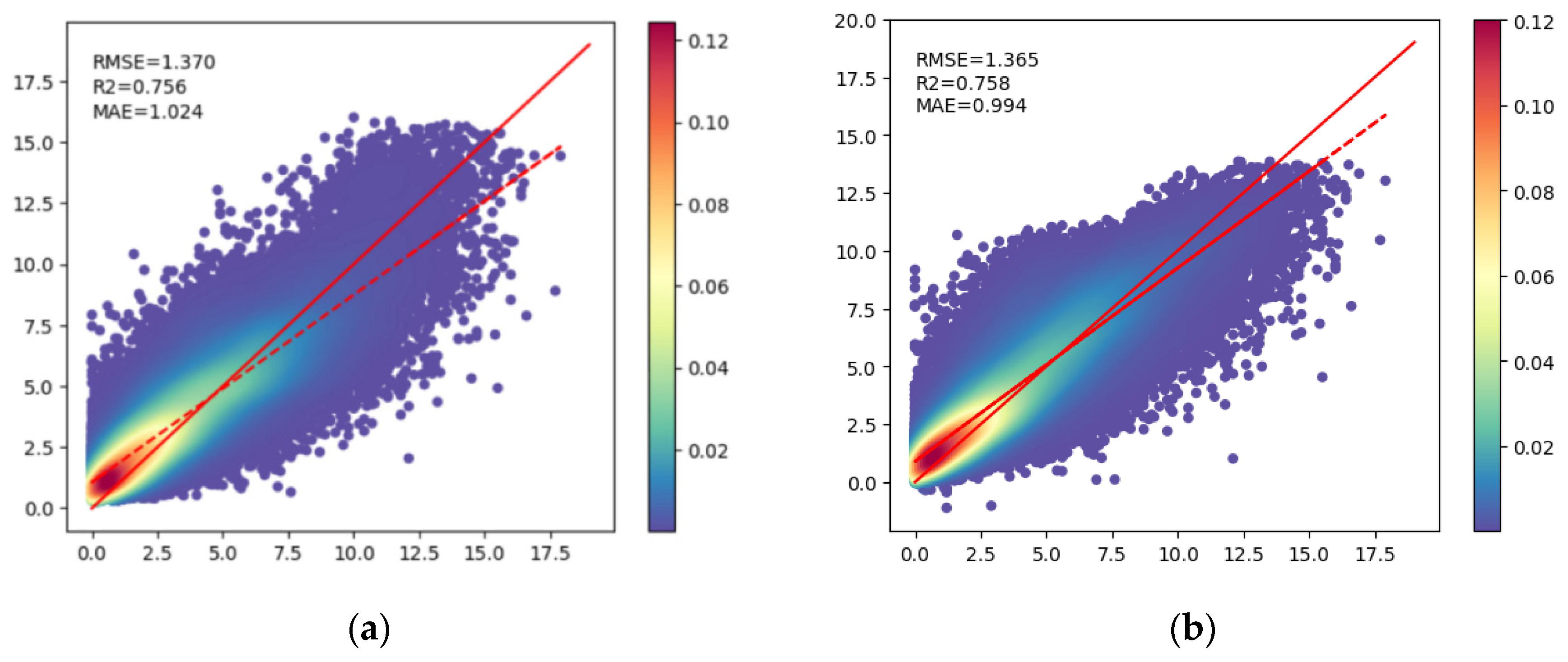
3.1. Evaluation of Spatial Accuracy

Each sample point in our dataset represents the measured evaporation for a particular meteorological station on a given day. We calculated the probability density of each sample point and organized these data into probability density distribution plots, as demonstrated in Figure 5. In these figures, red indicates the highest distribution density, while blue-purple signifies the lowest. We employed the least square method to fit the sample points, and the dotted lines represent the fitting effect. The accuracy evaluation metrics for the RF, SVM, ELM, CNN, and DNN models are provided in

Table 4. Model accuracy evaluation.

Model	RMSE	R2	MAE
RF	1.370	0.756	1.024
SVM	1.365	0.758	0.994
ELM	1.407	0.743	1.048
CNN	1.355	0.762	1.013
DNN	1.462	0.723	1.072

. The coefficient of determination, R², assesses the model’s goodness of fit, while the root mean square error (RMSE) and mean absolute error (MAE) measure prediction accuracy, with MAE being less influenced by outliers. The combined use of these three indicators can comprehensively assess the performance of the model in different aspects, and with this, we aim to provide a comprehensive understanding of the overall performance of the surface evaporation estimation model.

In summary, the model performance ranks as follows: CNN, SVM, RF, ELM, and DNN. The CNN demonstrated the most exceptional performance, boasting the highest R², the lowest RMSE, and the second-lowest MAE among the five models. In terms of training speed, the sequence is CNN, DNN, ELM, RF, and SVM, from fastest to slowest. Considering both model accuracy and training efficiency, the CNN model emerged as the top choice for producing surface evaporation data products encompassing the entire Yangtze River Basin from 2010 to 2019.

The CNN model exhibited the most favorable fitting effect, and the DNN model exhibited the least favorable fitting effect, so both were separately examined for changes in training performance with increasing iteration times.

The loss values of the CNN and DNN models evolved with the number of iterations, as illustrated in Figure 6. Notably, the loss value of the CNN model underwent a rapid decline and maintained stability as iterations progressed. Conversely, the loss value of the DNN model exhibited more pronounced fluctuations and did not reach a stable state with increasing iterations.

Within the CNN model, the R² values and RMSE values of variables such as LST, d2m, and lai_hv were calculated for different standard deviation percentage deviations, as presented in Figure 7. With this analysis, we aimed to gauge the extent to which changes in variables affect simulated evaporation. The figures reveal that the variables with the most substantial impact on simulated evaporation are strd, LST, d2m, and v10, with their influence ranked from highest to lowest.

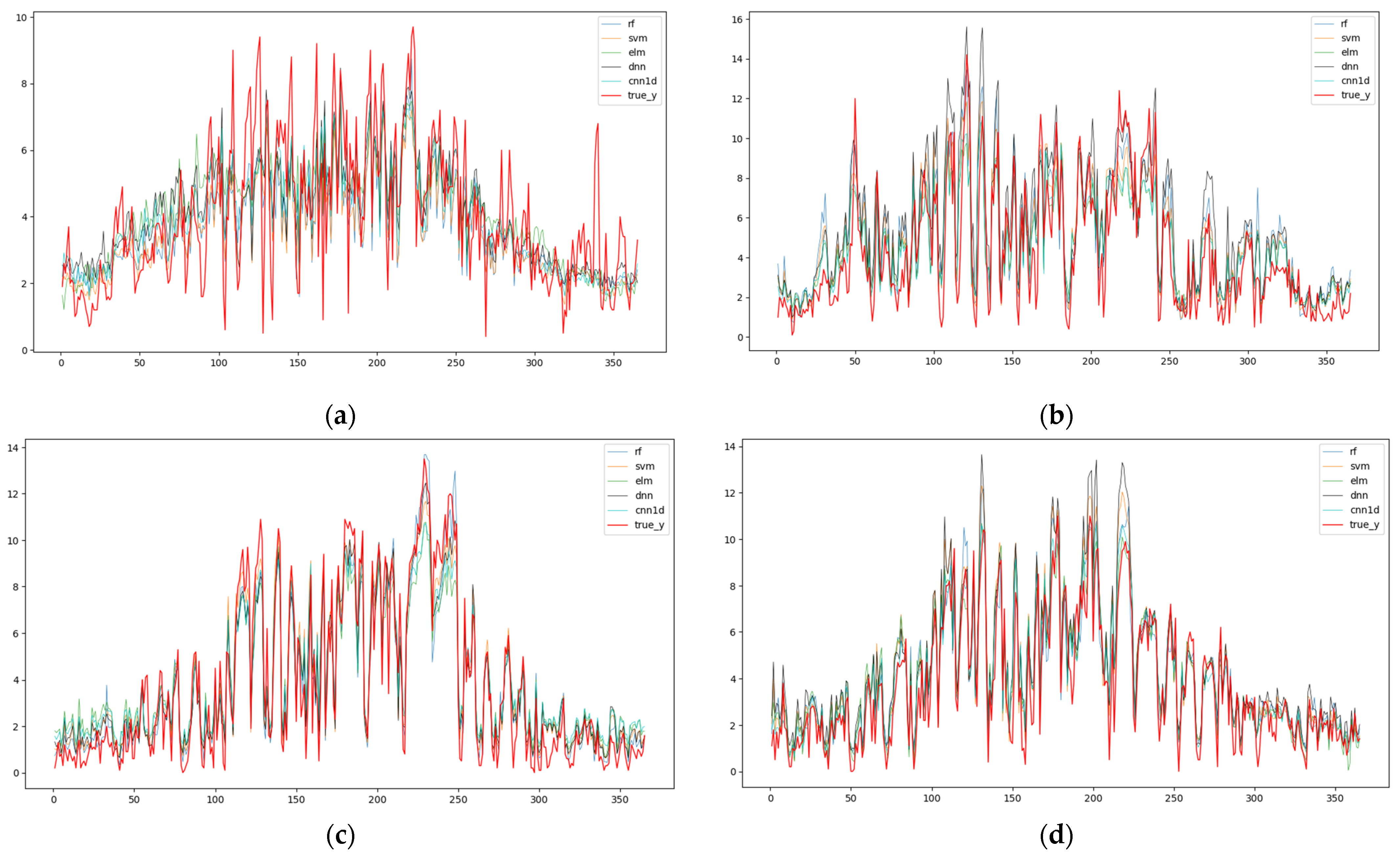
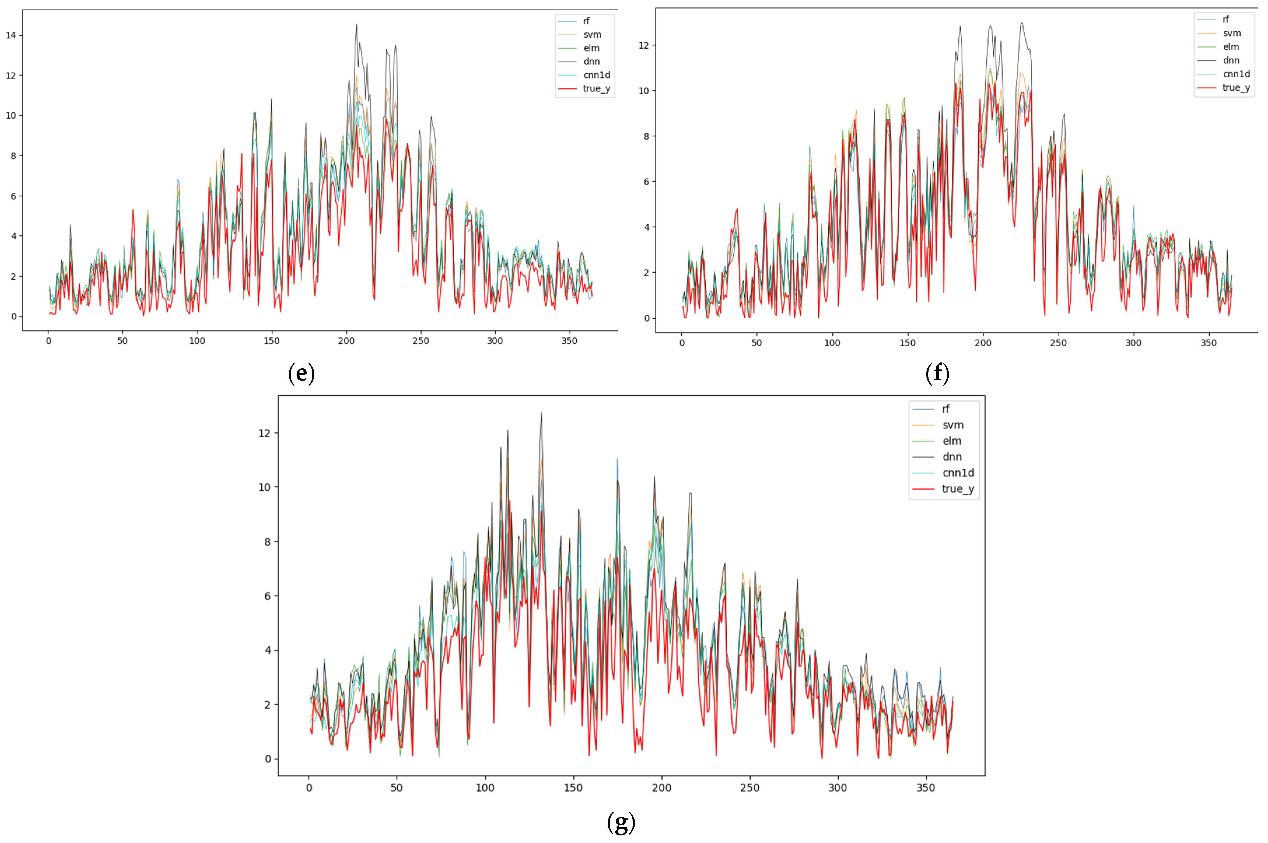
3.2. Evaluation of Temporal Accuracy

To see and analyze the differences between the estimated values and the real values of the five models, seven meteorological stations were selected (Nos. 56004, 56584, 57425, 57575, 57840, 57891, and 58237), and the data from 1 January 2010 to 31 December 2010 were plotted. Figure 8 shows the locations of the stations. The stations cover the Jinsha River Basin, the upper mainstream area of the Yangtze River, the middle stream area of the Yangtze River, the lower stream area of the Yangtze River, and some tributaries.

The measured evaporation values and model-predicted values based on the seven sites are shown in Figure 9, where the horizontal coordinate is time and the vertical coordinate is the evaporation amount.

The R² values of the five machine learning models at the seven meteorological stations are shown in

Table 5. The training effect of the five machine learning models at each meteorological station in 2011.

	RF	SVM	ELM	CNN	DNN
Station.56004	0.593	0.596	0.514	0.630	0.602
Station.56584	0.708	0.724	0.736	0.747	0.582
Station.57425	0.911	0.913	0.858	0.874	0.910
Station.57575	0.829	0.810	0.851	0.868	0.735
Station.57840	0.688	0.642	0.709	0.719	0.460
Station.57891	0.851	0.852	0.846	0.873	0.757
Station.58237	0.491	0.431	0.586	0.597	0.265

.

For each weather station, the model’s degree of fit is as follows, from highest to lowest: (1) Station 56004: CNN > DNN > SVM > RF > ELM; (2) Station 56584: CNN > ELM > SVM > RF > DNN; (3) Station 57425: SVM > RF > CNN > ELM > DNN; (4) Station 57575: CNN > ELM > RF > SVM > DNN; (5) Station 57840: CNN > ELM > RF > SVM > DNN; (6) Station 57891: CNN > SVM > RF > ELM > DNN; (7) Station 58237: CNN > ELM > RF > SVM > DNN. Except for Station No. 57425, during the period from 1 January 2010 to 31 December 2010, the R² value of the CNN model at six of the stations was the highest, indicating the best-fitting effect. At Station 57425, the R² value of the CNN model was only 0.004 below the maximum value. Apart from Station 56004, the DNN model had the poorest fit among six of the stations. Among all seven stations, the model’s degree of fit is as follows, from highest to lowest: CNN > SVM ≈ ELM ≈ RF > DNN. The performance of SVM, RF, and ELM at different stations had advantages and disadvantages. This aligns with the overall evaluation of all meteorological stations in the Yangtze River Basin, where the order was CNN > SVM > RF > ELM > DNN.

Except for the subpar performance of the DNN model at Station 57840 and the subpar performance of the RF, SVM, and DNN models at Station 58237, the predicted evaporation from the five machine learning methods closely matched the actual evaporation at these sites. However, compared with the measured values, it is apparent from the figures that the predicted values of all the models were generally overestimated to some extent, especially during the time range of 180–240 days. This may be attributable to the high summer temperatures and surface temperatures, causing the actual evaporation to approach the upper limit of the pan measurement.

The performance of the models is listed as follows, from best to worst: CNN, SVM, RF, ELM, and DNN. The fastest-to-slowest training speeds of the models are CNN, DNN, ELM, RF, and SVM. The CNN model excels in both model accuracy and training speed. When compared with the measured evaporation values, the predictions of all five models exhibit a certain degree of overestimation, especially during the summer. With its hierarchical structure, the CNN model can efficiently extract features from complex spatiotemporal data, enhancing accuracy. Its weight-sharing mechanism can capture spatial correlations, contributing to both accuracy and fast training. Modeling nonlinear relationships ensures enhanced accuracy without compromising training speed. The CNN’s adaptability to complex spatial structures in the Yangtze River Basin ensures accurate predictions with efficient training. Consequently, we chose the CNN model to produce surface evaporation data products for the Yangtze River Basin from 2010 to 2019.

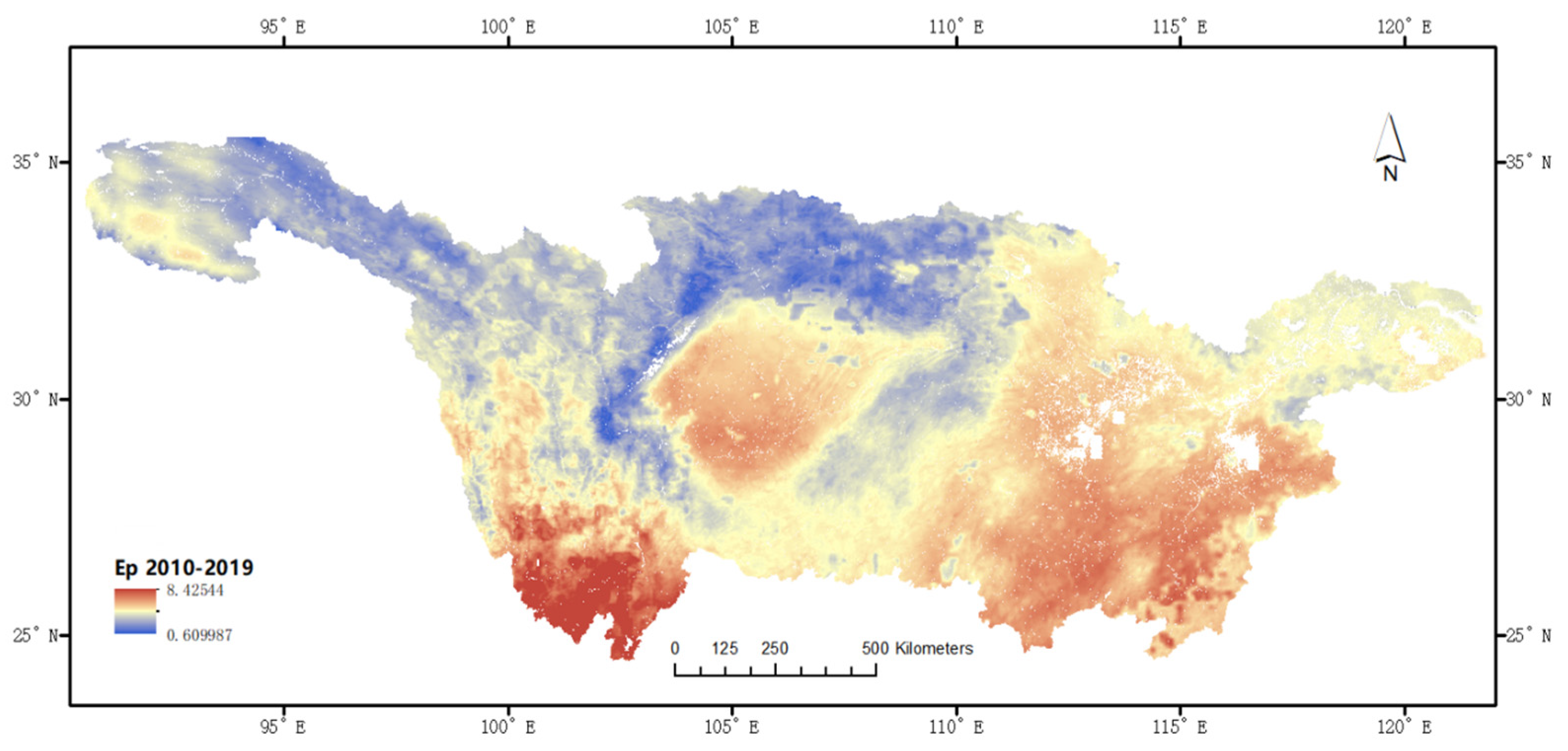
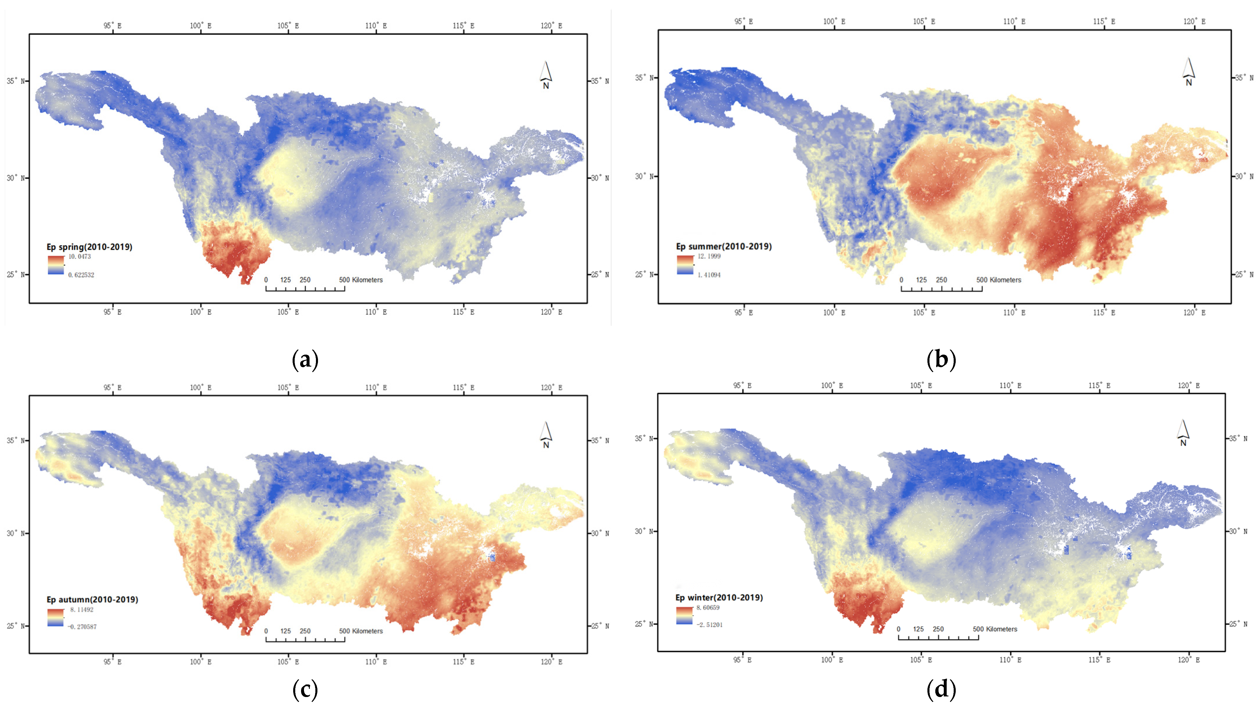
3.3. Analysis of Spatial Characteristics

Daily 2010–2019 data for surface evaporation, meteorological, and radiation variables in the Yangtze River Basin in Figure 10 exhibited spatial heterogeneity, revealing regional disparities. High evaporation regions are concentrated in the lower Jinsha River, the Poyang Lake Basin, the Dongting Lake Basin, and some upper Yangtze River areas. Conversely, low evaporation regions are mainly found in the upper Jinsha River, the northwestern Minjiang River Basin, the northern Jialing River Basin, and the northwestern Hanjiang River Basin because of higher elevations.

Higher evaporation in the lower Jinsha River is due to elevated net solar radiation, wind speed, and temperature. In Poyang Lake and the southeastern Dongting Lake Basin, higher evaporation is primarily associated with elevated temperature, although the net surface radiative flux also plays a significant role. The upper reaches of the Yangtze River experience increased evaporation because of elevated temperatures and moderate wind speed.

Lower evaporation in the upper Jinsha River is linked to lower temperatures and higher net heat radiation. The northwestern Minjiang River Basin, the northern Jialing River Basin, and the northwestern Hanjiang River Basin exhibited lower evaporation because of lower wind speeds and medium-to-low surface net solar radiation.

A spatial autocorrelation test using the Global Moran’s I Index was conducted on daily average evaporation data from 2010 to 2019 for the Yangtze River Basin. The results revealed high spatial autocorrelation, indicating that evaporation in the basin is influenced significantly by neighboring areas. The analysis identified multiple high and low evaporation value clusters across the basin.

Figure 11 highlights high-value cluster regions in the southwestern Yangtze River Basin, including Chuxiong, Lijiang, Kunming, and Panzhihua. Eastern Sichuan and western Chongqing also exhibited high-value cluster regions. The largest high-value region spans western Jiangxi and Hunan. These regions have significantly higher evaporation than average, distributed independently. A high–low cluster area surrounds the eastern part of Sichuan and western Chongqing, extending to the middle of Guizhou, western Hunan, northern Hunan, and on to Anhui and Shanghai. This region features a high-value area associated with a low-value region. In contrast, the western low–high cluster region covers the central and western parts of Sichuan, which are characterized by lower overall values but associated with a high-value region. Low–low areas are found in southern Gansu, Shaanxi, central Sichuan, and the upper reaches of the Jinsha River in Qinghai, where evaporation is significantly lower than average.

3.4. Analysis of Temporal Characteristics

Distribution maps of daily average evaporation for different seasons within the Yangtze River Basin are shown in Figure 12. Missing data in these maps are the result of incomplete ERA5 data.

The average daily evaporation pattern across the seasons is as follows: summer > autumn > spring > winter. In summer, the average daily evaporation ranges from 1.41094 to 12.1999 mm. Autumn exhibits an average daily evaporation between −0.270587 and 8.11492 mm. Spring’s average daily evaporation falls within a range of 0.622532 to 10.0473 mm, while winter has the lowest average daily evaporation, varying between −2.51201 and 8.60659 mm.

Summer has the highest average daily evaporation. Spatially, there are significant variations in summer evaporation. The Jinsha River Basin, the northwestern Minjiang River Basin, and the northern Jialing River Basin differ markedly from other regions. The former experiences low evaporation values, while the latter has higher values. In regions outside the Jinsha River Basin, evaporation generally decreases gradually from the southeast to the northwest.

Although spring’s average daily evaporation has higher maximum and minimum values compared with autumn, the high-evaporation area in autumn is larger. In autumn, this area is primarily concentrated in the lower reaches of the Jinsha River, the Poyang Lake Basin, and the southeastern part of the Dongting Lake Basin. In spring, the high-evaporation area is limited to the upper reaches of the Jinsha River Basin, specifically where the Jinsha River and the Yalong River converge in northern Yunnan and southern Sichuan.

Winter has the lowest average daily evaporation among the four seasons. Its spatial distribution pattern aligns with spring, albeit with lower overall values.

The monthly surface evaporation data for 1 km of the Yangtze River Basin from 2010 to 2019 were computed using the CNN model and subjected to trend analysis.

Trend analysis was performed using the pymannkendall package in Python, which provided various results, including the trend itself (significant increase, significant decrease, or no trend), the existence of the trend, standardized test statistics, Kendall Tau, variance, Sen’s Slope, and intercept. The primary focus was placed on the trend, p-value, and slope variables.

In the visualization (Figure 13, Figure 14 and Figure 15), areas with no significant trends are shown in gray. The trends, regional distribution of significant and very significant changes, and Sen’s Slope distribution of evaporation in the Yangtze River Basin are displayed.

The trend distribution in Figure 13 exhibits three cases: significant decrease, significant increase, and insignificance. Most areas displayed no significant changes. A significant decrease was observed in the northwest (the upper reaches of the Jinsha River), specifically near the Tongtian River in Qinghai Province. Significant increases were found in parts of the upper reaches of the Yangtze River, including the eastern mainstream area, the northwestern Jialing River Basin, the northeastern Bintuo River Basin, the northwestern upper mainstream area of the Yangtze River, and sporadic areas of the Jinsha River Basin.

Figure 14 details significant and very significant changes in evaporation, denoting different levels of significance (gray for not significant, green for significant, and red for very significant). The Jialing River Basin and some upper mainstream areas experienced a significant increase in this trend. Conversely, the headwater region of the Yangtze River exhibited a significant decline in evaporation.

Sen’s Slope values for regions with significant evaporation changes are presented in Figure 15, ranging from −0.227746 to 0.556789. A positive Sen’s Slope indicates an upward trend in evaporation from 2010 to 2019, while a negative value represents a downward trend.

This study’s spatial distribution analysis sheds light on the pronounced heterogeneity of surface evaporation exhibited across the Yangtze River Basin. This insight underscores the interconnected nature of surface evaporation in the basin. Temporal analysis showed notable seasonal variations, with summer exhibiting the highest daily average evaporation rates. This observation is crucial for understanding regional hydrological cycles and water resource management.

4. Conclusions

In this study, we selected ERA5 data, a 1 km seamless surface temperature dataset in China, and a daily surface climate dataset to estimate surface evaporation in the Yangtze River Basin using five different machine learning algorithms. Site-based spatial accuracy evaluations and time series analysis were conducted. The primary work and conclusions of this study are as follows:

■

Comparative analysis of five machine learning methods for estimating surface evaporation in the Yangtze River Basin:

We used random forest (RF), support vector machines (SVM), extreme learning machines (ELM), convolutional neural networks (CNN), and deep neural networks (DNN) to estimate surface evaporation at 234 meteorological station locations in the Yangtze River Basin from 2010 to 2019. We chose 13 variables as feature inputs based on prior knowledge and correlations and used evaporation pan measurements as the output variable. The results indicated that the CNN model exhibited the best performance among the methods in terms of fitting and training speed.

■

Generation of daily, 1 km surface evaporation data for the Yangtze River Basin using a convolutional neural network:

• In the spatial distribution analysis, the surface evaporation displayed notable spatial variations in the basin, indicating higher evaporation in the southwestern and southeastern regions compared with the western and northern areas.
• Spatial autocorrelation analysis using the Global Moran’s I index suggested significant spatial dependencies, revealing multiple high and low aggregation areas within the basin.
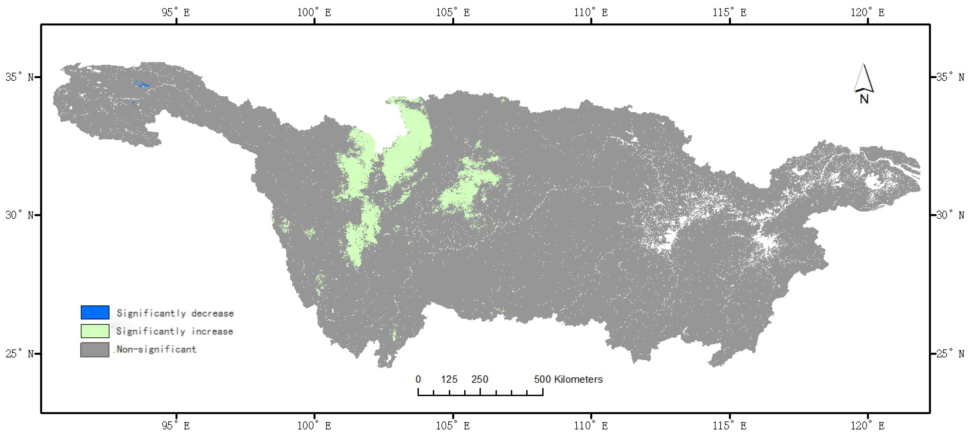
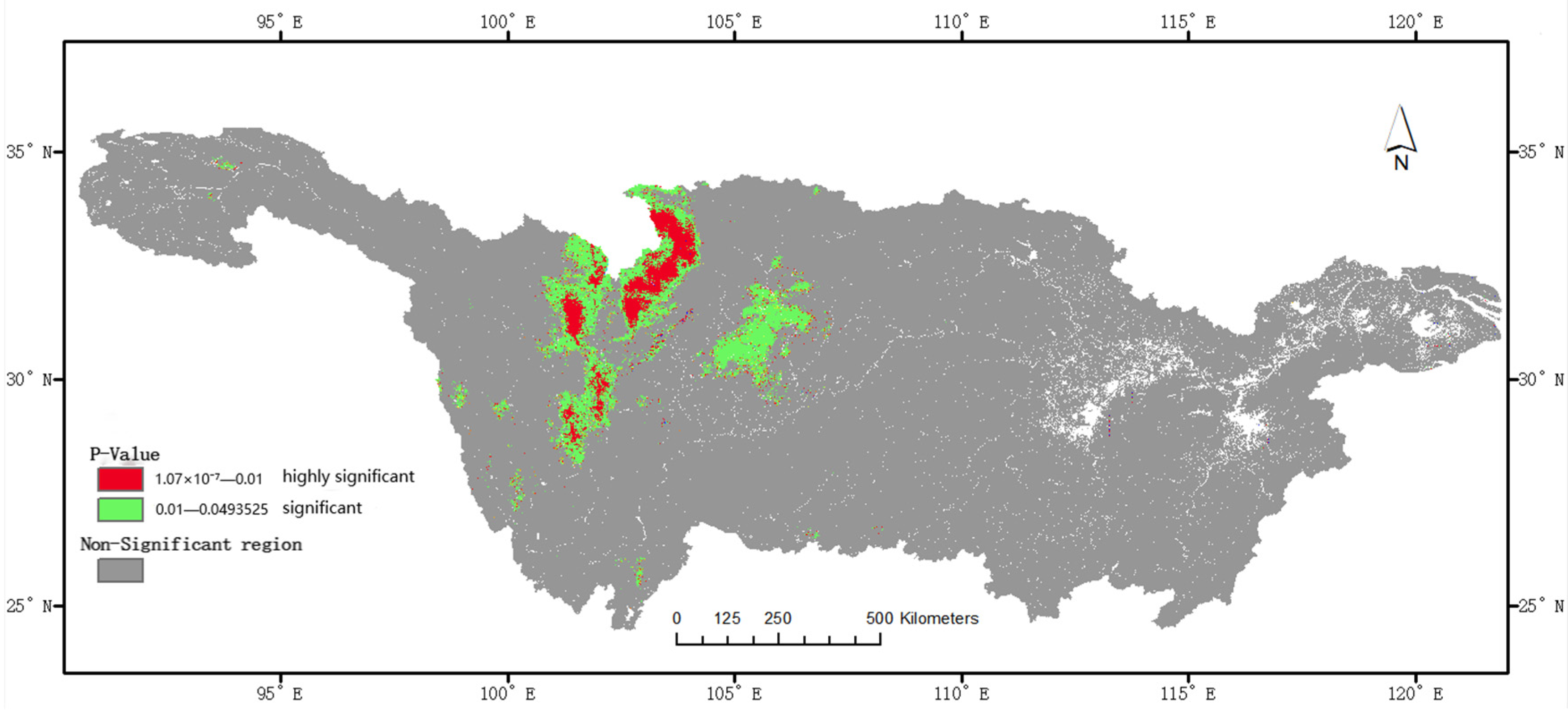
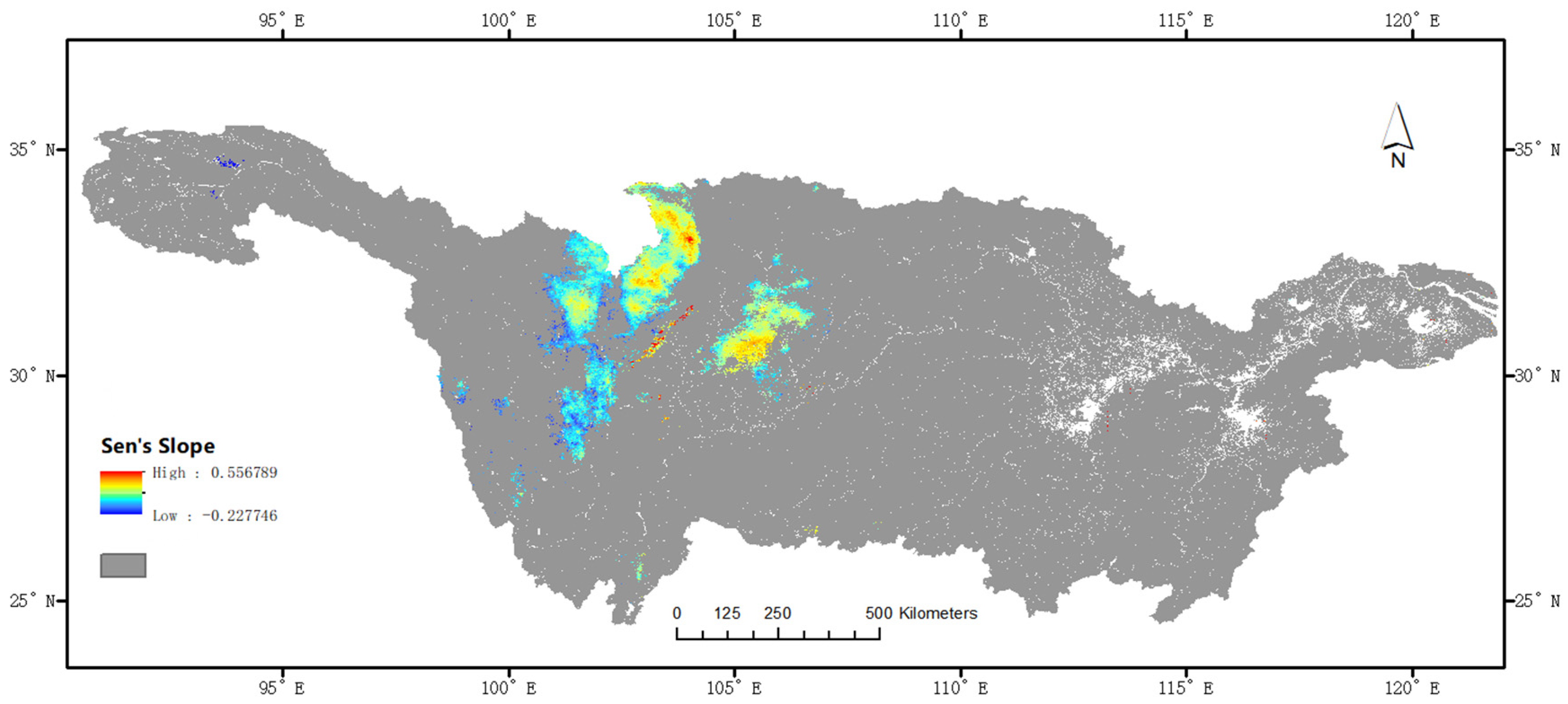
• A time series analysis of seasonal and monthly evaporation data revealed a general trend of higher evaporation in summer compared with other seasons, with certain areas showing a significant increase or decrease in evaporation over ten years. These changes varied spatially, with a notable increase in specific parts of the basin, mainly in the Jialing River Basin.

This study’s outcomes provide insights into the complexity of factors influencing evaporation in the Yangtze River Basin, emphasizing both spatial and temporal variations in surface evaporation. In the future, we will explore the causes and effects of temporal and spatial variations in surface evaporation. For instance, a quantitative analysis examining the relationship between evaporation, rainfall, flood disasters, and drought disasters can be integrated to elucidate their interdependencies.

References

1. Liu, B.; Xu, M.; Henderson, M.; Gong, W. A spatial analysis of pan evaporation trends in China, 1955–2000. J. Geophys. Res. Atmos. 2004, 109, D15. [Google Scholar] [CrossRef]
2. Ye, L.; Lu, H.; Qin, S.; Zhang, L.; Xiong, L.; Liu, P.; Xia, J.; Cheng, L. Changes in pan evaporation and actual evapotranspiration of the Yangtze River basin during 1960—2019. Adv. Water Sci. 2022, 33, 718–729. [Google Scholar] [CrossRef]
3. Liu, M.; Tang, R.; Li, Z.; Maofang, G.; Yunjun, Y. Progress of data-driven remotely sensed retrieval methods and products on land surface evapotranspiration. Natl. Remote Sens. Bull. 2021, 25, 1517–1537. [Google Scholar] [CrossRef]
4. Fan, J.; Wu, L.; Zhang, F.; Xiang, Y.; Zheng, J. Climate change effects on reference crop evapotranspiration across different climatic zones of China during 1956–2015. J. Hydrol. 2016, 542, 923–937. [Google Scholar] [CrossRef]
5. Shiri, J.; Kişi, Ö. Application of Artificial Intelligence to Estimate Daily Pan Evaporation Using Available and Estimated Climatic Data in the Khozestan Province (South Western Iran). J. Irrig. Drain. Eng. 2011, 137, 412–425. [Google Scholar] [CrossRef]
6. Dong, L.; Zeng, W.; Wu, L.; Lei, G.; Chen, H.; Srivastava, A.K.; Gaiser, T. Estimating the Pan Evaporation in Northwest China by Coupling CatBoost with Bat Algorithm. Water 2021, 13, 256. [Google Scholar] [CrossRef]
7. Ding, R.; Kang, S.; Li, F.; Zhang, Y.; Tong, L.; Sun, Q. Evaluating eddy covariance method by large-scale weighing lysimeter in a maize field of northwest China. Agric. Water Manag. 2010, 98, 87–95. [Google Scholar] [CrossRef]
8. Xu, C.-Y.; Gong, L.; Jiang, T.; Chen, D.; Singh, V.P. Analysis of spatial distribution and temporal trend of reference evapotranspiration and pan evaporation in Changjiang (Yangtze River) catchment. J. Hydrol. 2006, 327, 81–93. [Google Scholar] [CrossRef]
9. Wang, Y.; Jiang, T.; Bothe, O.; Fraedrich, K. Changes of pan evaporation and reference evapotranspiration in the Yangtze River basin. Theor. Appl. Climatol. 2007, 90, 13–23. [Google Scholar] [CrossRef]
10. Rong, Y.S.; Zhang, X.N.; Jiang, H.Y.; Bai, L.Y. Pan Evaporation Change and Its Impact on Water Cycle over the Upper Reach of Yangtze River. Chin. J. Geophys. 2012, 55, 488–497. [Google Scholar]
11. Lu, X.; Ju, Y.; Wu, L.; Fan, J.; Zhang, F.; Li, Z. Daily pan evaporation modeling from local and cross-station data using three tree-basedmachine learning models. J. Hydrol. 2018, 566, 668–684. [Google Scholar] [CrossRef]
12. Chen, J.L.; Yang, H.; Lv, M.Q.; Xiao, Z.L.; Wu, S.J. Estimation of monthly pan evaporation using support vector machine in Three Gorges Reservoir Area, China. Theor. Appl. Climatol. 2019, 138, 1095–1107. [Google Scholar] [CrossRef]
13. Xu, S.; Cheng, J. A new land surface temperature fusion strategy based on cumulative distribution function matching and multiresolution Kalman filtering. Remote Sens. Environ. 2021, 254, 112256. [Google Scholar] [CrossRef]
14. Zhang, Q.; Wang, N.; Cheng, J.; Xu, S. A Stepwise Downscaling Method for Generating High-Resolution Land Surface Temperature From AMSR-E Data. IEEE J. Sel. Top. Appl. Earth Obs. Remote Sens. 2020, 13, 5669–5681. [Google Scholar] [CrossRef]
15. Zhang, Q.; Cheng, J. An Empirical Algorithm for Retrieving Land Surface Temperature From AMSR-E Data Considering the Comprehensive Effects of Environmental Variables. Earth Space Sci. 2020, 7, e2019EA001006. [Google Scholar] [CrossRef]
16. Cheng, J.; Dong, S.; Shi, J. 1 km Seamless Land Surface Temperature Dataset of China (2002–2020); National Tibetan Plateau/Third Pole Environment Data Center: Beijing, China, 2021. [Google Scholar]
17. Breiman, L. Random Forests. Mach. Learn. 2001, 45, 5–32. [Google Scholar] [CrossRef]
18. Svetnik, V.; Liaw, A.; Tong, C.; Culberson, J.C.; Sheridan, R.P.; Feuston, B.P. Random Forest:  A Classification and Regression Tool for Compound Classification and QSAR Modeling. J. Chem. Inf. Comput. Sci. 2003, 43, 1947–1958. [Google Scholar] [CrossRef] [PubMed]
19. Hearst, M.A.; Dumais, S.T.; Osuna, E.; Platt, J.; Scholkopf, B. Support vector machines. IEEE Intell. Syst. Their Appl. 1998, 13, 18–28. [Google Scholar] [CrossRef]
20. Huang, G.B.; Zhu, Q.Y.; Siew, C.K. Extreme learning machine: Theory and applications. Neurocomputing 2006, 70, 489–501. [Google Scholar] [CrossRef]
21. Guang-Bin, H.; Qin-Yu, Z.; Chee-Kheong, S. Extreme learning machine: A new learning scheme of feedforward neural networks. In Proceedings of the 2004 IEEE International Joint Conference on Neural Networks (IEEE Cat No04CH37541), Budapest, Hungary, 25–29 July 2004. [Google Scholar]
22. Abed, M.; Imteaz, M.A.; Ahmed, A.N.; Huang, Y.F. Modelling monthly pan evaporation utilising Random Forest and deep learning algorithms. Sci. Rep. 2022, 12, 13132. [Google Scholar] [CrossRef]
23. Gu, J.; Wang, Z.; Kuen, J.; Ma, L.; Shahroudy, A.; Shuai, B.; Liu, T.; Wang, X.; Wang, G.; Cai, J.; et al. Recent advances in convolutional neural networks. Pattern Recognit. 2018, 77, 354–377. [Google Scholar] [CrossRef]
24. Keskin, M.E.; Terzi, Ö. Artificial Neural Network Models of Daily Pan Evaporation. J. Hydrol. Eng. 2006, 11, 65–70. [Google Scholar] [CrossRef]
Figure 1. Technology roadmap.
Remotesensing 16 00057 g001
Figure 2. Model variable correlation coefficient heat map.
Remotesensing 16 00057 g002
Figure 3. CNN model structure.
Remotesensing 16 00057 g003
Figure 4. One-dimensional CNN model structure.
Remotesensing 16 00057 g004
Figure 5. (a) RF model probability density map; (b) SVM model probability density map; (c) ELM model probability density map; (d) CNN model probability density map; (e) DNN model probability density map.
Remotesensing 16 00057 g005aRemotesensing 16 00057 g005b
Figure 6. (a) Loss diagram of CNN model; (b) loss diagram of DNN model.
Remotesensing 16 00057 g006
Figure 7. (a) R2 values of each variable of the CNN model at different percentages of standard deviation; (b) RMSE values of each variable of the CNN model at different percentages of standard deviation.
Remotesensing 16 00057 g007
Figure 8. Location map of meteorological stations.
Remotesensing 16 00057 g008
Figure 9. (a) Time series chart showing evaporation at meteorological station 56004 in 2011; (b) time series chart showing evaporation at meteorological station 56584 in 2011; (c) time series chart showing evaporation at meteorological station 57425 in 2011; (d) time series chart showing evaporation at meteorological station 57575 in 2011; (e) time series chart showing evaporation at meteorological station 57840 in 2011; (f) time series chart showing evaporation at meteorological station 57891 in 2011; (g) time series chart showing evaporation at meteorological station 58237 in 2011.
Remotesensing 16 00057 g009aRemotesensing 16 00057 g009b
Figure 10. Distribution map of mean evaporation in the Yangtze River basin in ten years.
Remotesensing 16 00057 g010
Figure 11. High and low cluster map of mean evaporation in the Yangtze River basin over ten years.
Remotesensing 16 00057 g011
Figure 12. (a) Distribution of daily mean evaporation in spring in the Yangtze River Basin; (b) distribution of daily mean evaporation in summer in the Yangtze River Basin; (c) distribution of daily mean evaporation in autumn in the Yangtze River Basin; (d) distribution of daily mean evaporation in winter in the Yangtze River Basin.
Remotesensing 16 00057 g012
Figure 13. Trend distribution map of evaporation in the Yangtze River Basin from 2010 to 2019.
Remotesensing 16 00057 g013
Figure 14. Distribution map of significant and highly significant evaporation changes in the Yangtze River Basin during 2010–2019.
Remotesensing 16 00057 g014
Figure 15. Sen’s Slope distribution of evaporation in the Yangtze River Basin from 2010 to 2019.
Remotesensing 16 00057 g015