Abstract
The indoor geometric dimensions of a building are crucial for acceptance criteria. Traditional manual methods for measuring indoor geometric quality are labor-intensive, time-consuming, error-prone, and yield non-reproducible results. With the advancement of ground-based laser scanning technology, the efficient and precise measurement of geometric dimensions has become achievable. An indoor geometric quality measurement method based on ground-based laser scanning is presented in this paper. Initially, a coordinate transformation algorithm based on selected points was developed for conducting coordinate conversion. Subsequently, the Cube Diagonal-based Denoising algorithm, developed for point cloud denoising, was employed. Following that, architectural components such as walls, ceilings, floors, and openings were identified and extracted based on their spatial relationships. The measurement and visualization of the geometric quality of walls’ flatness, verticality, and opening dimensions were automated using fitting and simulation methods. Lastly, tests and validation were conducted to assess the accuracy and applicability of the proposed method. The experimental results demonstrate that time and human resources can be significantly saved using this method. The accuracy of this method in assessing wall flatness, verticality, and opening dimensions is 77.8%, 88.9%, and 95.9%, respectively. These results indicate that indoor geometric quality can be detected more accurately and efficiently compared to traditional inspection methods using the proposed method.
1. Introduction
The indoor geometric quality measurement of building projects aims to check whether the construction discrepancies are within the allowable ranges of the national housing construction specifications [1]. The measurement scope covers the concrete structure, masonry structure, plastering, waterproofing, doors and windows, coating, fine decoration, and other processes.
The indoor wall flatness [2,3,4], verticality, and dimensions of the door and window openings, which not only affect the appearance of the building but also reflect the quality and characteristics of the construction, are important measurement indexes during construction. However, the current basic and commonly used acceptance inspection methods involve measuring the elevation of selected points using tools such as calipers, 2 m rulers, and optical levels and comparing them with the design elevations. Alternatively, inclinometers and other measurement instruments are used to measure the elevation difference between two points to represent flatness [2,3,4,5,6,7]. Nevertheless, the use of traditional measuring tools like measuring tapes [8,9,10], spirit levels, and instruments is often labor-intensive, time-consuming, and prone to errors due to manual intervention [11,12,13]. Traditional measurement methods are heavily reliant on the subjective experience of workers, and non-compliance during the construction and handover phases can result in costly rework. Previous statistics have shown that 54% of construction defects are attributed to inexperienced workers or other subjective factors, while 12% are caused by systemic issues [14]. Therefore, it is essential to regularly measure geometric quality during construction. As indoor acceptance requirements in construction continue to rise, traditional manual inspection methods are unable to meet the increasing demands [7]. Consequently, there is an urgent need for an automated method to measure indoor geometric dimensions.
Currently, more advanced tools are used for geometry measurement, such as handheld laser rangefinders, which use lasers to measure the distance to the target. To ensure the accuracy of the measurement, the instrument should preferably be rotated from a fixed position to complete the measurement, and all measurement points must be perpendicular or parallel to the plane during the measurement process. Therefore, measurement using a handheld laser rangefinder can replace traditional measuring tape, but it cannot realize non-contact automatic measurement and effective precision control and has obvious limitations. In addition, a slope meter [6] and other measuring instruments are used to measure the elevation difference between a pair of points to express the flatness information. The level gauge and total station can greatly improve the accuracy and speed of a single measurement, but the measurement results are not comprehensive enough, and the measurement process fails to overcome the defects caused by manual measurement. The above more advanced measurement methods are still manually conducted, meaning they are still time-consuming, subjective, and inaccurate [6,15,16]. Therefore, to solve the above problems and adapt to the trend of automated measurement, a new efficient and automated solution is necessary.
The proliferation of 3D capture devices, such as Light Detection and Ranging (LiDAR) and depth cameras, has provided researchers from various industries with an unprecedented interest in point cloud processing. Point cloud data are disordered collections of points, which are created in 3D space by accessing accurate location information on the surface of the scanned object [17,18,19,20,21,22]. Point cloud data can usually be accessed from multiple data sources [23,24], such as laser scanning [25,26,27,28], images [24], and videos [29]. In the past ten years, point cloud data collection processes have become more mature. The 3D point cloud data from sensing technology have a higher measurement rate and better measurement accuracy than traditional measurement methods and are used by various industries to increase productivity. Three-dimensional laser scanning is also known as real-world replication technology or LiDAR, which breaks through the method of single-point measurement and has the unique advantages of higher efficiency and high-precision acquisition. According to the working platform, three-dimensional laser scanning can be subdivided into three categories, namely Terrestrial Laser Scanning (TLS), Airborne Laser Scanning (ALS), and Mobile Laser Scanning (MLS) [30]. Among the above three types, TLS has the highest measurement accuracy due to its relatively static measurement method and is more widely used in high-precision measurement applications. In the construction industry, 3D point cloud data have become the preferred choice for providing accurate geometric information for construction projects and for improving decision making. Three-dimensional point cloud data are widely used in the construction phase of prefabricated buildings and the maintenance phase of building bridges [31], which mainly include 3D model reconstruction and quality detection [4,11,25,32,33,34,35].
Some researchers [36,37,38] studied the reconstruction of 3D models, which obtains the spatial coordinates of each point on the component surface. Then, the spatial information is transformed into digital information that can be directly processed using computing equipment. Various algorithms were developed [39,40] to complete the calculation and visualization of indoor geometric quality based on this digital information. However, there are still some problems in the accuracy and comprehensiveness of the previous algorithms, which only stay in the initial stage of theory application and are not able to be effectively applied in practice. There are few exploratory studies on indoor wall verticality and door or window opening dimension measurement. Therefore, inspired by the actual measurement process of wall flatness, wall verticality, and door or window opening dimensions by experienced workers on site, as well as related specifications and previous research, the goal of this study is to propose an automatic measurement method of the indoor geometric quality including flatness, verticality, and door or window opening dimensions.
The main contributions of this study are summarized as follows: (1) Based on the proposed coordinate transformation method, this paper proposes the Cube Diagonal-based Denoising algorithm for fine denoising method to eliminate noise in the interior space of the room and attached to the plane, achieving the goal of fine denoising. (2) On the basis of the proposed coordinate transformation point cloud, this article extends the region growth segmentation algorithm to make the semantic recognition and segmentation of ceilings, floors, and walls more efficient. (3) This article provides a comprehensive visualization of the detection results for the key indicators in the actual measurement of dimensions in the entire room, which can provide clearer and more convenient guidance for operators to locate size defects.
The remaining parts of this study are organized as follows: Section 2 introduces the acquisition and applications of point cloud data in the related fields. Section 3 and Section 4, respectively, describe the method scheme of this study and related experiments to verify the proposed method through an actual residential indoor environment. Section 5 discusses and summarizes this study and puts forward the directions and suggestions for future study.
2. Related Works
2.1. Data Acquisition
Many previous studies have proven that TLS has good applicability in the field of construction measurement. TLS mainly uses two different principles for measurement: time of flight (TOF) and phase shift. The principle of TOF is as follows: TLS emits laser pulses and measures the time of flight of the reflected pulses, and the distance can be calculated based on the known speed of light. The other is the phase shift principle: TLS emits an amplitude-modulated continuous wave (AMCW), then measures the phase shift between the transmitted signal and the reflected signal. The distance value can be calculated based on the wavelength [30]. The TOF method, which is generally used for engineering measurement, has a longer measurement distance (up to 6000 m) and millimeter-level accuracy, while the phase-shift method has a higher measurement speed. It is necessary to determine the location and scanning parameters of the TLS before the scanning work. The three main factors that affect the accuracy of the TLS measurement are as follows: (1) distance, (2) incident angle between TLS and the target structure, and (3) angular resolution. After the position and parameters are determined, automatic scanning begins, with the scanner’s head undergoing horizontal and vertical rotation [41]. The scanned data of each measurement position contain a set of (X, Y, Z) values, which can accurately locate the relative position of points. TLS has been widely used in different fields due to its significant advantages over traditional measurement tools, including cultural relic protection [42,43], earthwork volume measurement [44,45], topographic survey [46], and construction progress tracking [47,48].
2.2. TLS-Based Geometric Quality Detection
Before TLS was widely used in concrete geometric quality detection, there was research on the automated detection of concrete surface and geometric quality based on images. For example, based on Bayesian decision theory, Hutchinson et al. [49] used statistical methods to analyze the images and then obtain the image analysis results of concrete cracks. Zhu [50] used images to identify key structural defects and used related algorithms to identify and repair column members. However, these image-based detection methods required the assistance of a large number of two-dimensional images, and image segmentation or geometric detection techniques of feature points and lines were used to evaluate the quality of the detected target [51]. High-resolution images are required in these studies. Therefore, image-based methods have obvious limitations and are not suitable for residence scene detection.
Later, TLS and related point cloud algorithms played an important role in the geometric quality detection of construction scenes, overcoming the shortcomings of images. For example, some studies [52,53,54] have focused on comparing point cloud models to BIM models to accomplish detection. This method consumes a lot of time to create the model in the early stage and cannot guarantee the accuracy of the BIM model, so it cannot ensure the proper accuracy of registration and comparison calculation. Bosché and Guenet [39] compared the TLS data with the design model and used the F-number method to automatically evaluate the flatness of walls [40,55,56]. The accuracy of the data was good, but the validity of the F-value of the manual measurement data failed to be verified. Shih and Wang [57] used the TLS to define the scanned wall plane as a reference plane and expressed the flatness information of the wall using the moving method. However, because the detection is completed in a mobile manner, the detection accuracy failed to be guaranteed within the millimeter range. Bosché and Biotteau [3] used two more advanced technologies, namely TLS and continuous wavelet transform, to detect and visualize the flatness information of manually selected area surfaces and to compare the measurement results with the wave index. The results show a high correlation and seem robust, but further research based on the wavelet transform and related requirements is still needed to confirm the accuracy of this method. Tang et al. [4,58] defined a framework to evaluate the performance of different scans and effectively used TLS to implement, verify, and compare three algorithms for the detection of plane flatness. The results show that the study can effectively express the flatness defects, but the limitation is that there is no plane fluctuation to comprehensively characterize the surface flatness. Akinci et al. [12] proposed the first formal method to integrate project 3D models and sensor systems (especially TLS) for construction quality control, which is called defect detection and characterization. However, the method requires a lot of manual work when generating as-built models. Bosche [59] proposed an automated method to identify 3D CAD objects from laser scanning data for the dimensional compliance check of building components. However, this method still needs the as-designed model, which increases the work of manual intervention. Other TLS-based quality assessment studies of concrete structures mainly focus on detecting damages, such as large cracks, flatness, and spalling [25,28,38,39]. For the measurement of openings, Zolanvari et al. [60] proposed the improved slicing method (ISM) as an extension to the initial slicing method (ISM) for processing point cloud data, and identified the position of openings. The efficiency of detecting the opening positions is good, but no further study has been performed on the dimensions of these openings. Li et al. [61] calculated the verticality of the wall by calculating the angle between the normal vector of the wall and the ground, but this method only uses two vectors to represent the whole plane, which does not meet the standard requirements in the actual measurement process, and the calculation results are crude and inaccurate.
In summary, the past research on the measurement of indoor geometric quality mainly focused on the measurement of a single index, the studies of verticality and openings are scarce, and the visualization of measurement results is not comprehensive or intuitive. Many related works need heavy manual work and as-designed models to assist measurement work, which do not meet both the standard of manual measurement and the requirement of comprehensive visualization. Therefore, this study will directly calculate, analyze, and visualize the measurement of flatness, verticality, and opening dimensions based on the real scanning point cloud data and directly benchmark with the requirements of manual measurement specifications so that the results are more accurate and reliable. The detailed methodology is presented in the following sections.
3. Proposed Automated Indoor Geometric Quality Assessment Method
This section describes the automated measurement and visualization method of the three indexes: flatness, verticality, and door or window opening dimensions. The measurement target of this study is a residential indoor room, which includes walls (including door and window openings), ceiling, and floor. The premise of this study is that the civil engineering construction has been completed in its entirety, and it has progressed to the stage before interior decoration. At this stage, site clearing and related operations have already been conducted, resulting in minimal interference or obstructions present on the site. Before commencing the scanning process, appropriate algorithms are used for site planning to ensure the completeness of room scanning. Furthermore, it ensures that point cloud data can be automatically registered during the scanning process. Subsequently, manual semantic segmentation is performed on the scanned rooms, with the calculations and visualization processes being automated using this method.
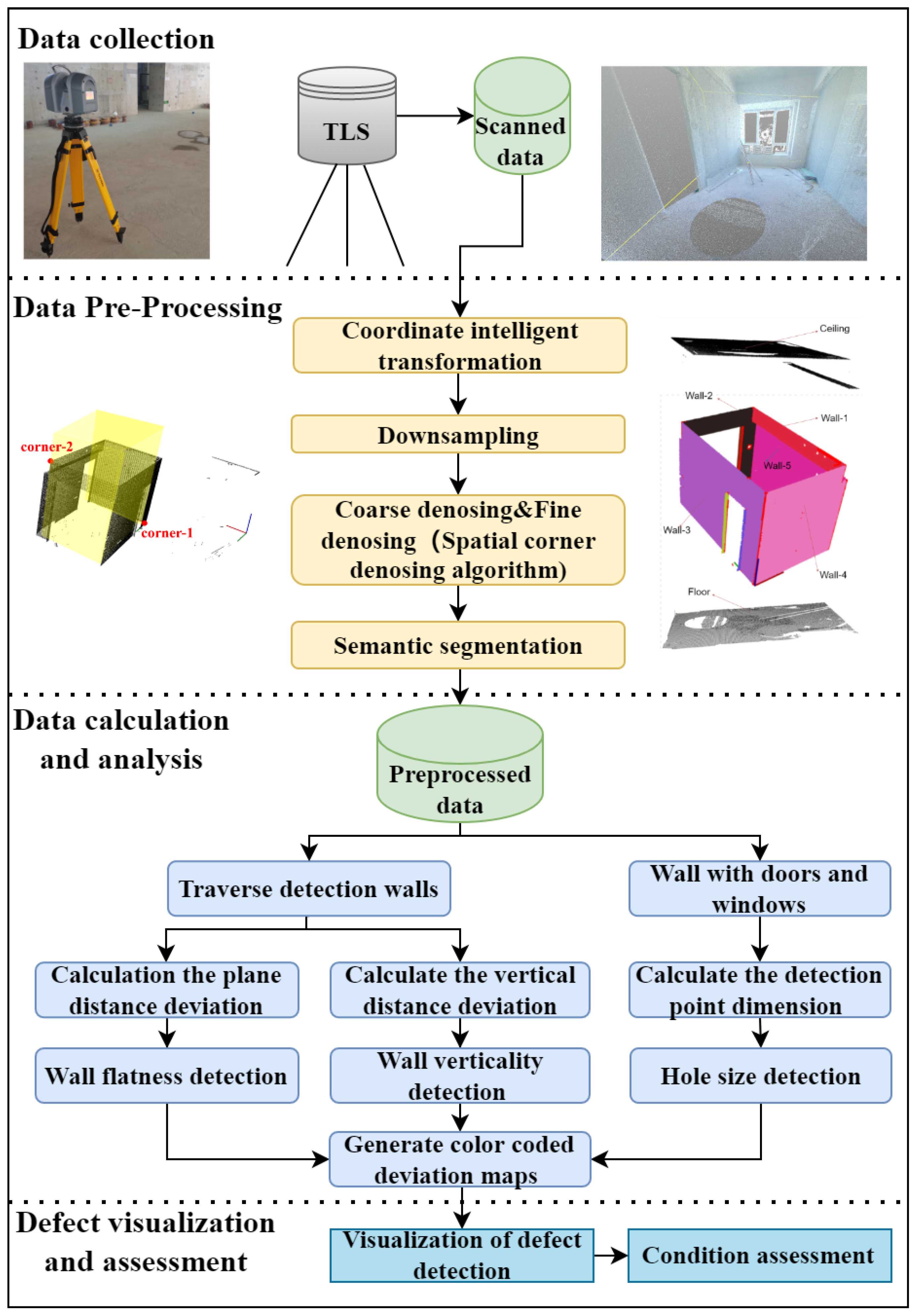
As shown in Figure 1, the flowchart of the proposed method is summarized. Firstly, this study preprocesses the original data after inputting the point cloud data of a room. Preprocessing steps include coordinate transformation, down-sampling, denoising, and semantic segmentation. Secondly, the algorithm mainly refers to the actual measurement process and specifications of indoor geometric quality to automatically calculate and measure the related geometric indexes based on the orientation characteristic relationship between different target planes. Thirdly, using the calculation results, the values and positions of the relevant measurements are visualized through automatically generated color coding and other techniques, making the results more intuitively clear. The above steps will be explained in Section 3.1 and Section 3.2, respectively, and the calculation process and visual definition of measurement results in each stage of the proposed method will be introduced in detail.

Figure 1.
The flowchart of the developed measurement method.
3.1. Data Acquisition and Preprocessing
This study uses TLS to acquire 3D point cloud data of the target room through on-site scanning. Generally, the data obtained using the scanning device are extremely numerous, with millions of points in a room [62], but the scanned data contains a lot of noise points that affect the calculation process. To avoid data redundancy and the calculation burden, the original collected data need to be preprocessed. The data preprocessing is completed in four steps: (1) coordinate transformation, (2) data down-sampling, (3) coarse denoising and fine denoising, and (4) semantic segmentation.
3.1.1. Coordinate Transformation
The conversion between scanned data and a custom platform coordinate system has always been a challenge. Typically, it is necessary to ensure that the coordinate systems of scanned data and the operating platform are parallel to each other on the XY plane and consistent in the Z-axis direction. A rigid transformation is performed to move and rotate the original point cloud to the custom coordinate system without altering the original size and geometric features. To ensure the accuracy of calculations, it is required that the origin of the original point cloud coincides with the origin of the operating platform. The transformation method proposed by Kim et al. faces difficulties in accurately identifying feature points [63] and has a high requirement for noise removal [41].
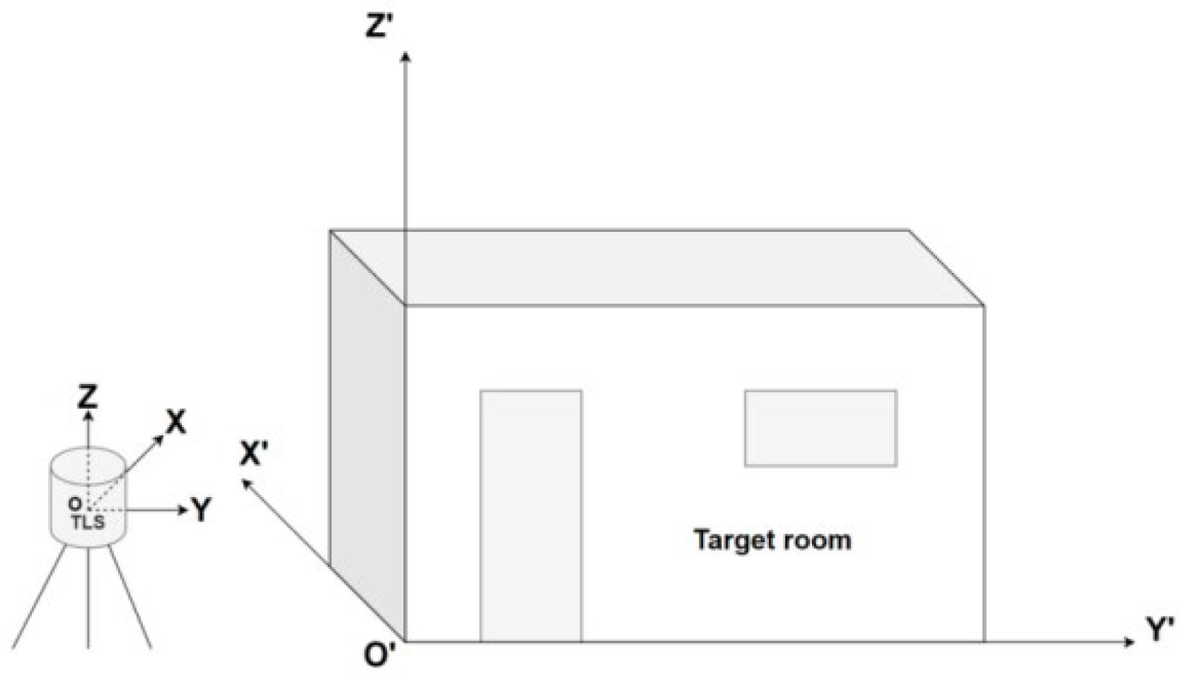
To meet the needs of this research, this study proposed a new coordinate trans-formation algorithm. Figure 2 shows the general orientation relationship of the point cloud data scanned using TLS and the coordinate system defined by the platform. There are large deviations between the two systems in the X-axis, Y-axis, and Z-axis, which may cause problems for the calculations of subsequent algorithms.
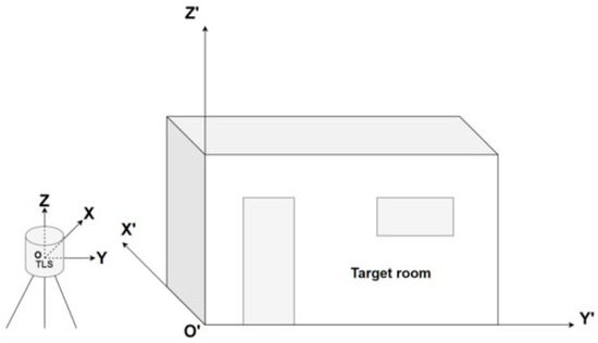
Figure 2.
The coordinate orientation relationship between TLS and target room.
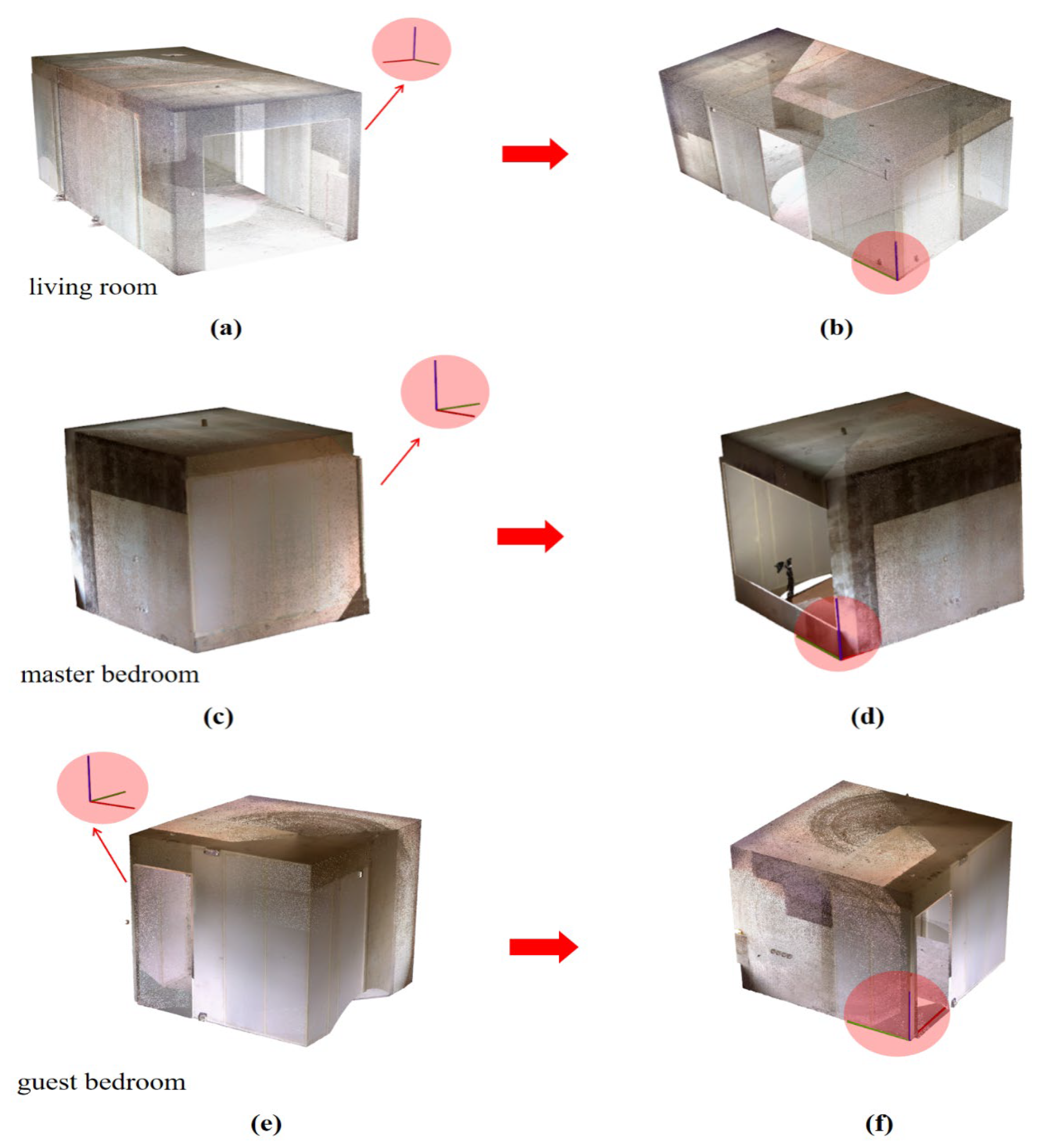
In this study, a new coordinate transformation algorithm is developed, which can directly and simply transform the 3D point cloud data rather than being based on the uncertain two-dimensional image, points, or line extraction. The specific steps are as follows: (1) the point cloud data of the original TLS coordinate system is loaded (Figure 3a). (2) In practice, there are multiple corners in the target room that can be defined as the origin of a user-defined coordinate system. Therefore, a 3D-type point picking event is defined as follows: a corner point is selected on the target room as the point coincident with the origin. Specifically, when clicking the selected point, which is shown in red, the algorithm automatically accesses the coordinate orientation of the selected point in the custom coordinate system (Figure 3b). (3) The (X, Y, Z) values of all original point coordinates are automatically subtracted from the (X, Y, Z) values of the selected point and the rigid transformation is performed (Figure 3c). (4) The other point on the transformed point cloud data is selected, and this selected point should be roughly on the same horizontal plane as the first red point and on the line rejoined with the X-axis according to Equation (1):
where θ is the required rotation angle, v1 is a unit vector in the X-axis, and v2 is the direction vector of the second selected point. The algorithm automatically calculates the angle between the orientation vector of the selected point and the X-axis and transfers the angle information to the defined rotation matrix, which automatically rotates the entire target at this angle (Figure 3d). In actual construction, indoor walls cannot be completely perpendicular to each other, so the rotated target (Figure 3e) will not perfectly coincide with the axis. The rotated target will inevitably have a deviation in the positive orientation of the axis, but it does not affect the purpose of coordinate transformation and the calculation of indexes. The coordinate transformation algorithm is simple, direct, and has robust applicability.
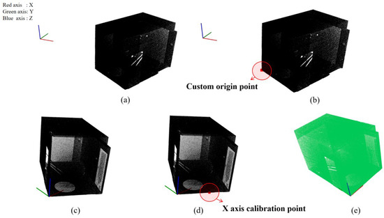
Figure 3.
The process of coordinate transformation, (a) original TLS coordinate system: loaded point cloud data, (b) user-defined coordinate system: 3D point picking, (c) coordinate transformation: rigid transformation, (d) automatic rotation: angle information transferred to rotation matrix, (e) rotated target: impact of wall angles on axis orientation.
3.1.2. Down-Sampling
At present, there are many down-sampling methods for point cloud data [64,65,66], which are usually used to reduce data redundancy. The main down-sampling algorithms applied to point cloud data are Farthest Point Sampling (FPS) [67], Normal Space Sampling (NSS) [68], and Voxel Grid Down-sampling (VGD) [69].
Because the resolution of the TLS is high, the number of original points in a room can reach millions, and the interval of points can even reach 1 mm. Through the above summary and research on the main down-sampling methods of the current point cloud processing, it can be seen that the VGD algorithm can not only reduce the number of points and the burden of calculation but also ensure the shape characteristics of the data. Hence, VGD is suitable for down-sampling the original point cloud data in this study. Figure 4 shows the effect of down-sampling a room using the VGD algorithm when the three-dimensional voxel grid is set to 0.01 m.
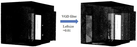
Figure 4.
The effect of VGD down-sampling.
3.1.3. Coarse Denoising and Fine Denoising
The purpose of this step is to reduce noise data from the down-sampled data. Data denoising is a critical step in data preprocessing as it directly affects the accuracy of subsequent calculations. However, the comprehensive removal of the noise points of the target is difficult in actual situations. In this study, the target room is denoised twice. The existing algorithm is used for the coarse denoising first, and then the developed algorithm is used for the fine denoising. The proposed algorithm still fails to guarantee the absolute removal of target noise points (target noise points in fine denoising) but can reduce the noise points attached to or inside the target to a large extent to meet the calculation requirements.
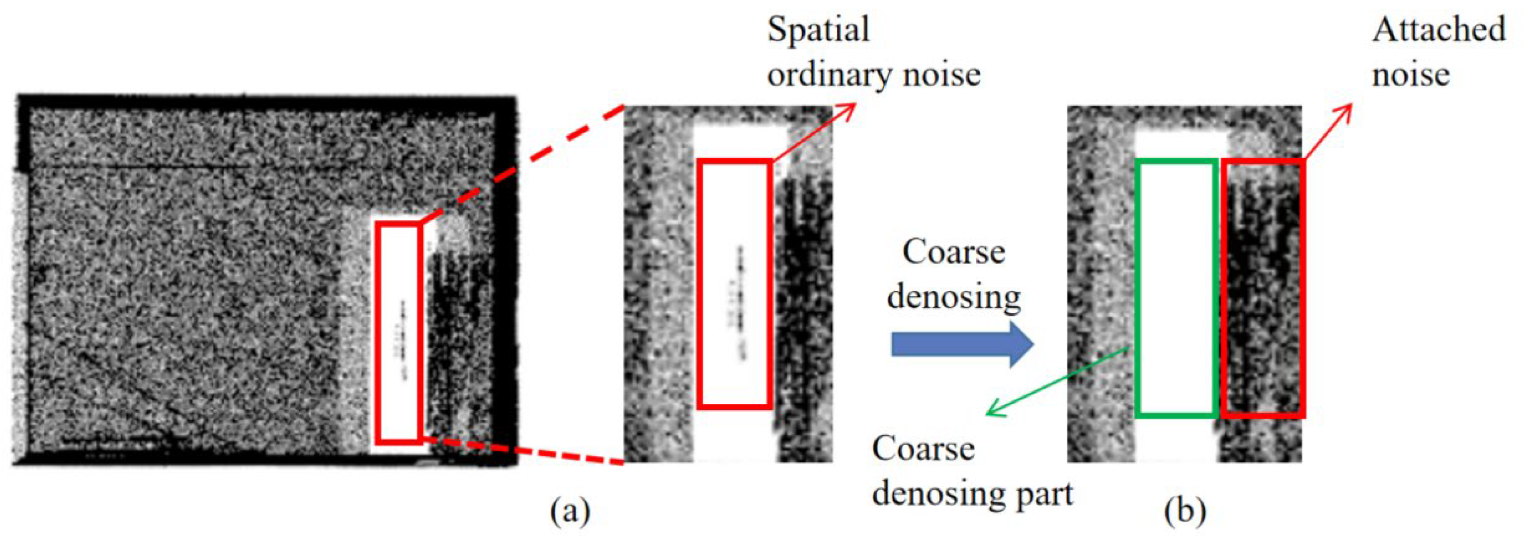
Firstly, the outlier feature is sparsely distributed in space, and the statistical outlier removal algorithm is used to remove obvious outliers. The algorithm defines that a point becomes invalid if its density is less than a certain value. The average distance from each point to its nearest k points is calculated, and the average distances of all points in the point cloud should form a Gaussian distribution. According to the given mean and variance, points outside the variance can be removed. The original noise points before coarse denoising are shown in the red box of Figure 5a, and the processing results are shown in Figure 5b. Obviously, the outliers in the red box of Figure 5a can be removed by means of coarse denoising. It can be clearly found that there are invalid points attached to the wall or floor, which are unnecessary and could affect the subsequent calculation and measurement (such as the residual noise points of the staff in the red box in Figure 5b), which need to be further removed.

Figure 5.
The statistical outlier removal denoising algorithm, (a) original noise points before coarse denoising: highlighted in red box, (b) coarse denoising results.
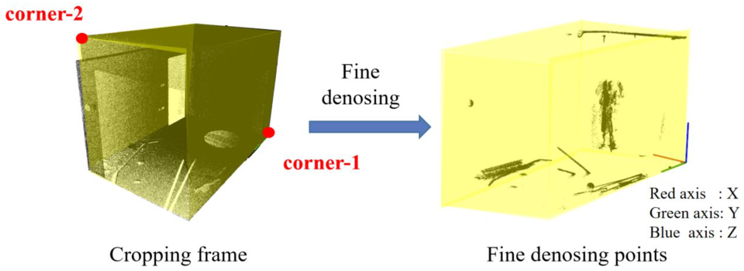
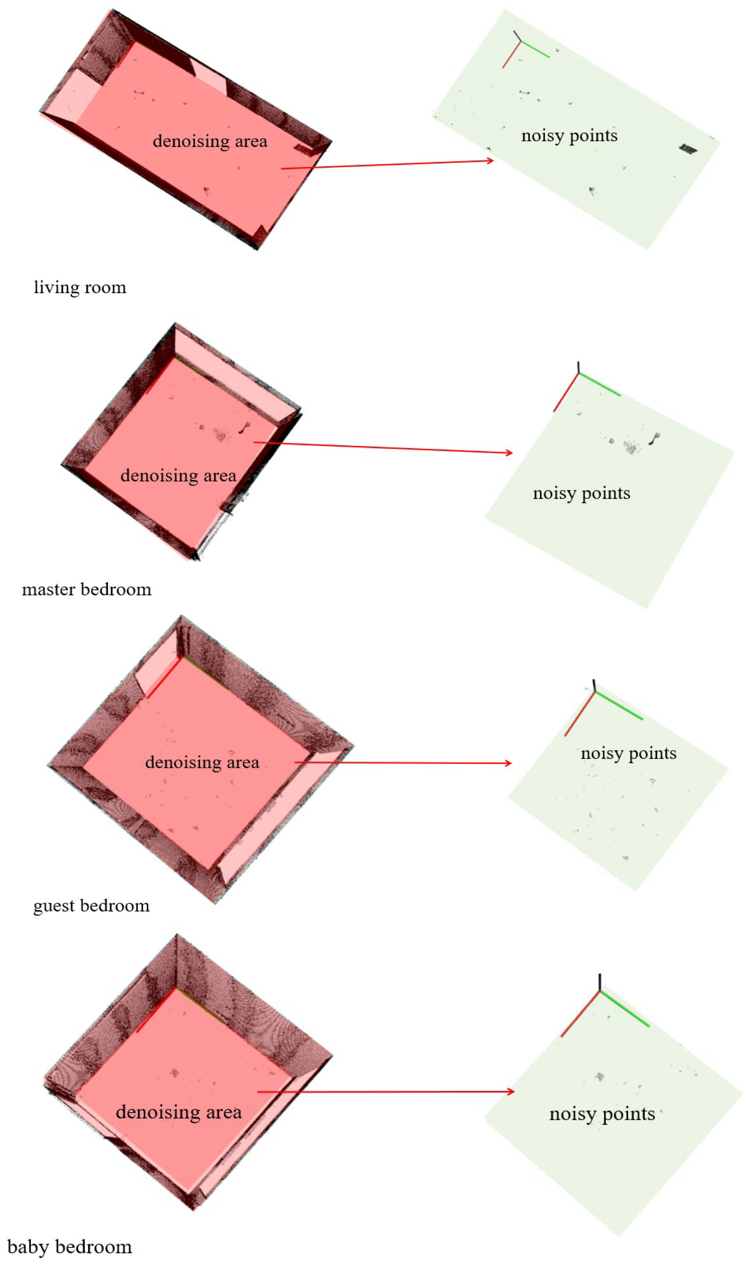
Based on a coarse denoising approach using statistical outlier removal algorithms, this study proposes a Cube Diagonal-based Denoising algorithm to further refine data denoising. The specific workflow of the algorithm is as follows: Firstly, define corner-1 as the corner point of the room near the coordinate axis origin on the ground. Then, define corner-2 as the diagonal corner point near the ceiling. Use these two corner points to create a 3D clipping cube. To ensure the geometric integrity of the walls and not affect the metric calculations, offset the entire clipping cube inward by an appropriate value based on the actual quality of the construction site data. When the clipping cube is separated from the walls, it remains fixed, and all points within the clipping cube are removed as unnecessary outliers. Figure 6 demonstrates the effects of the algorithm. While this algorithm may not completely eliminate all invalid outliers, it effectively removes noise points that do not belong to the target walls, largely meeting the calculation requirements.
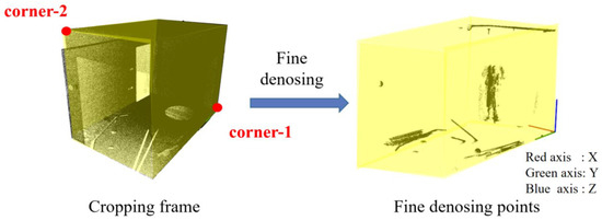
Figure 6.
The principle of the proposed Cube Diagonal-based Denoising algorithm.
3.1.4. Point Cloud Segmentation
Since the calculation of indexes needs to take a single plane as the object and semantically combine multiple objects, this method needs to save the ceiling, floor, and walls separately so that the developed algorithm can accurately identify the detection object. Firstly, all points are sorted according to the curvature values of all wall points. The point with the minimum curvature value is identified and added to the seed point set. For each seed point, the algorithm traverses the surrounding adjacent points and calculates the normal angle difference between each adjacent point and the seed point. The adjacent point is considered for subsequent detection if its difference is less than the threshold. The adjacent point is added to the seed point set if it meets the normal angle difference threshold and the curvature is less than the threshold, which proves that the adjacent point belongs to the current plane. Then, it should be noted that it is necessary to set the minimum cluster point number threshold to ensure that each identified plane contains an appropriate number of points until the cluster identified by the algorithm in the remaining points fails to meet the minimum point threshold.
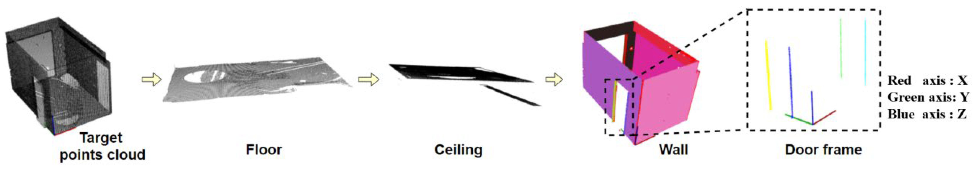
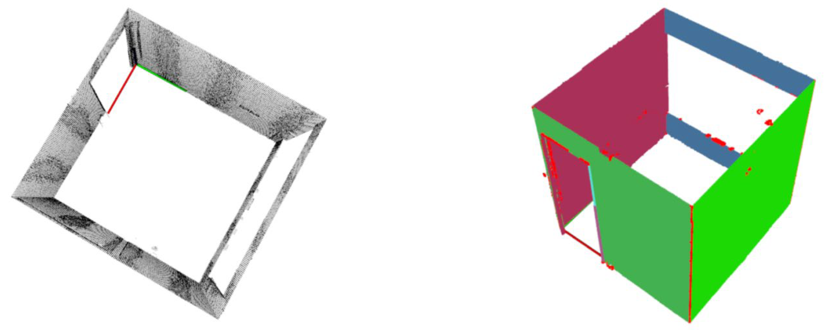
Finally, the region-growing segmentation algorithm is improved, and further judgment is made for each qualified cluster. The orientation conditions are set in the X-axis, Y-axis, and Z-axis orientations corresponding to each plane as follows: Firstly, the algorithm extracts the floor and ceiling plane. The clustered point cloud is identified as a floor or ceiling plane if it extends horizontally. The plane with the Z-values of cluster point clouds near the maximum Z-value of the whole room is identified as the ceiling, and the plane with the Z-values of cluster point clouds near the minimum Z-value of the whole room is identified as the floor. Then, the remaining data of the clustered point cloud that meet the extension threshold in the Z-axis orientation are further judged to be a wall plane. The cluster is discarded directly if it does not meet the extension threshold value. Otherwise, it is further determined whether the cluster meets the extension threshold value on the X-axis or Y-axis. The purpose of this step is to prevent unqualified clusters other than the walls from being recognized as a wall, such as the door frame in Figure 7. Finally, if the cluster meets the above threshold requirements, the target is automatically defined as the wall cluster and given a unique color for classification and semantic preservation. Figure 7 shows the process of segmentation.
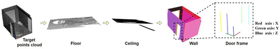
Figure 7.
The process of point cloud segmentation.
3.2. The Measurement and Visualization of Indoor Geometric Quality
Once the ceiling, floor, and walls of the room are semantically segmented through the above preprocessing, the proposed method traverses each plane cluster, extracts key geometric features, and measures the related geometric indexes. The measurement and visualization process of wall flatness, verticality, and door or window opening dimensions indexes will be introduced in detail below.
3.2.1. The Calculation and Visual Evaluation of the Wall Flatness Index
The essence of wall flatness detection is to define a reliable reference plane and calculate the distance deviation between the actual point cloud and the reference plane. Therefore, inspired by the work of Shih [57] and Li [2], this study further calculates and measures wall flatness with the essence of wall flatness measurement.
In the actual construction management, in addition to the consideration of safety performance, the construction cost is the first priority. The measures taken need to save the cost to the greatest extent if the defects are not enough to affect the safety. Therefore, based on the premise of safety, the wall is taken as the analysis object alone to access a more referential wall rather than be evaluated according to the control line of the construction drawing if the construction position of the whole wall is inaccurate. The reference plane should be able to more accurately represent the entire wall object, which means that most of the points should be on this plane.
Therefore, to accurately calculate the space equation of the plane and explain the spatial orientation of the target wall, the method traverses and fits each target wall. The previous method used the ordinary least squares method and the spatial plane equation of to fit the plane (singular value decomposition is used for ordinary least squares fitting), which is greatly affected by small error values, and the wall point cloud is very sensitive to the error value. Therefore, the RANSAC algorithm is used to complete wall fitting in this study. The RANSAC algorithm randomly selects a sample subset from the samples. The minimum variance estimation algorithm is used to calculate the model coefficients for this subset. The deviations between all samples and the model are calculated, and a preset threshold is used to compare with the deviation. The sample point is defined as belonging to the sample points inside the model (inliers) when the deviation is less than the threshold. Otherwise, the sample point is defined as belonging to the sample points outside the model (outliers). The current number of inliers is recorded, and the current best model coefficients are recorded in each repetition, which means that the number of inliers is the largest. At the time, the corresponding number of inliers is the best inliers. The end of each iteration is judged based on the expected error rate, best inliers, total number of samples, and current iteration times, and an iteration end evaluation factor is calculated, which means whether to end the iteration according to Equation (2).
where t is the proportion of “inliers” in the data, which is usually a prior value. The case where there is at least one “outer point” of the selected point is depicted by when n points are used in each calculation model, which means that in the case of k iterations, indicates that the calculation model samples at least one “outer point” to calculate the probability of the model. Then, the probability that the correct n points can be sampled to calculate the correct model is p, and k is the number of iterations required for the final calculation. To obtain more reliable parameters, the standard deviation or its multiplier is added to k. The standard deviation of k is defined as SD(k). After the iteration, the best model coefficients are the final model parameter estimations.
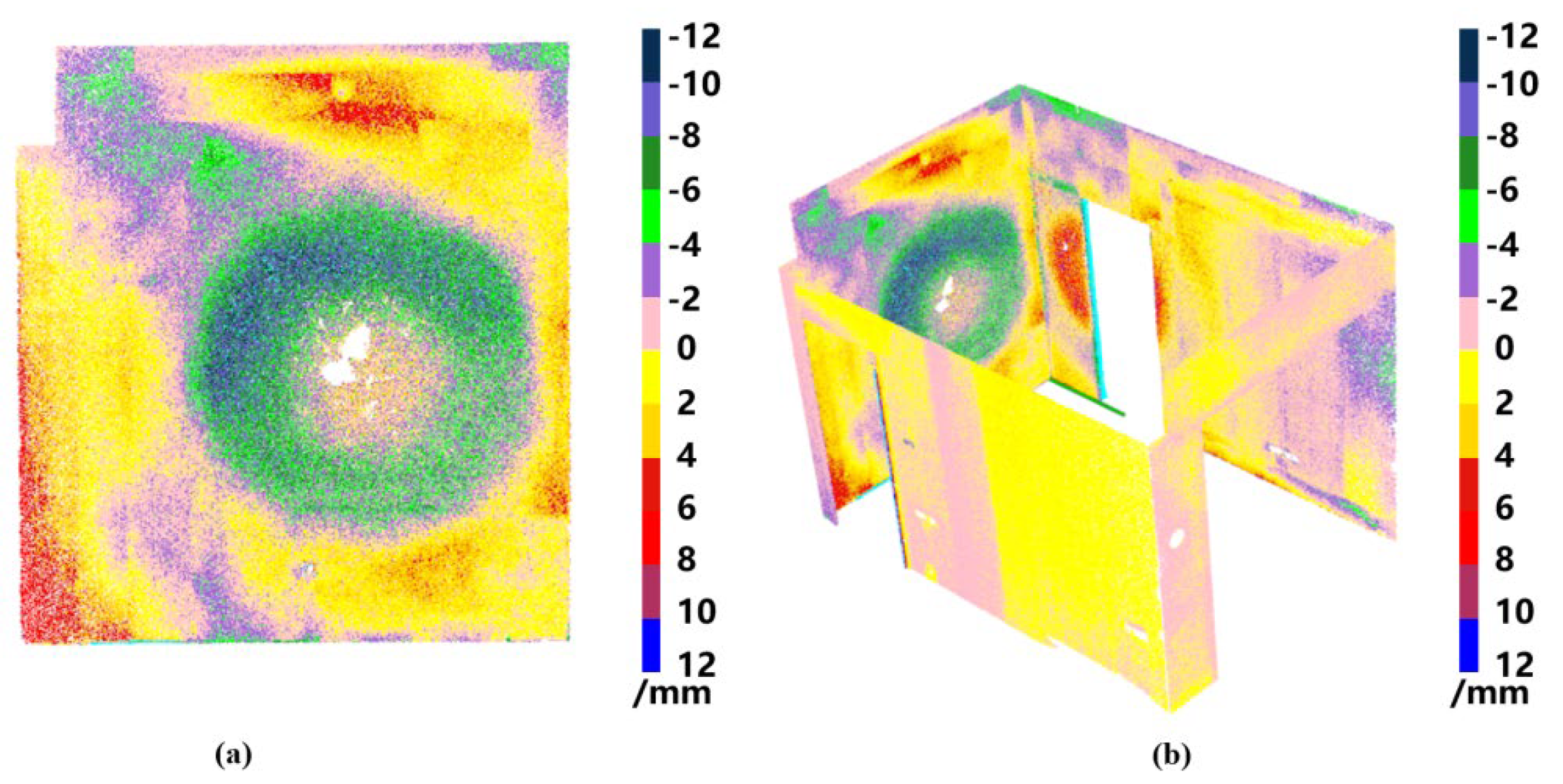
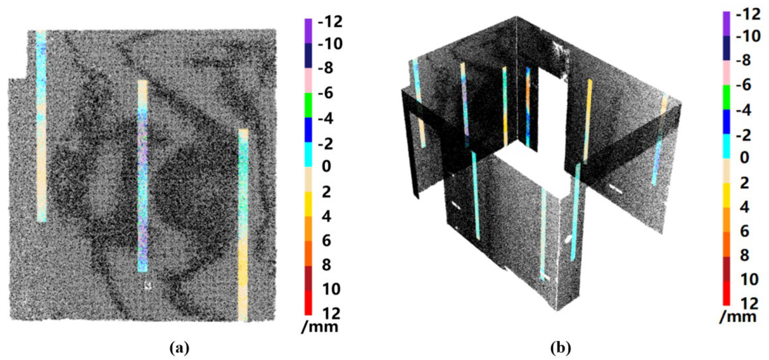
The experiments show that the coefficients of the equation change little after the arithmetic mean calculation of fitting three times. In order to fully reflect the characteristics of the plane, each wall is fitted five times in this study, and 90% of the points on each wall are randomly selected as fitting data for each fitting. The algorithm calculates the spatial plane equation after each fitting, and the coefficients of each randomly fitted plane are saved. After fitting five times, the arithmetic average calculation is completed based on the spatial plane equation coefficients of the five-fold fitting of each wall, and the most appropriate reference plane can be obtained. Then, the point-to-plane distance deviations between each point on the actual wall point cloud and the reference plane are calculated. The calculation principle is shown in Figure 8, and the normal vector outward from the wall plane is used as the positive orientation to judge whether the measurement part is convex or concave relative to the reference plane. To show the flatness quality of the wall plane more intuitively, each point is color-coded according to the positive and negative values of the distance deviation. The reference flatness qualification standard is 0 mm, 8 mm (plastering). In this study, the color interval is −12 mm, 12 mm, and each 2 mm between the areas is divided into a discontinuity so that the quality of each area of the wall can be intuitively and comprehensively reflected. For example, as shown in Figure 9a, the calculation result of the green part is negative, which means that the area is raised to the interior of the room; the calculated value is in the −4 mm, −6 mm range, which means that the area is raised to the interior by 4–6 mm. The changing trend of the whole wall’s flatness can also be clearly observed in the figure. The flatness information of the target wall can be viewed freely in three dimensions and can be rotated, enlarged, or shrunk arbitrarily. Finally, the relative orientation of the flatness cloud map of each wall in the room can be reorganized to comprehensively view the flatness of the wall in three dimensions, as shown in Figure 9b.
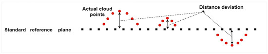
Figure 8.
The flatness calculation principle.
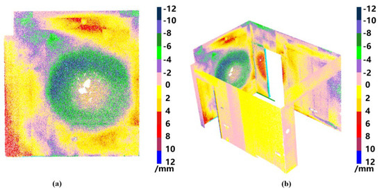
Figure 9.
The cloud map of flatness measurement: (a) wall flatness calculation result; (b) three-dimensional visualization of wall flatness cloud map.
3.2.2. The Calculation and Visual Evaluation of the Wall Verticality Index
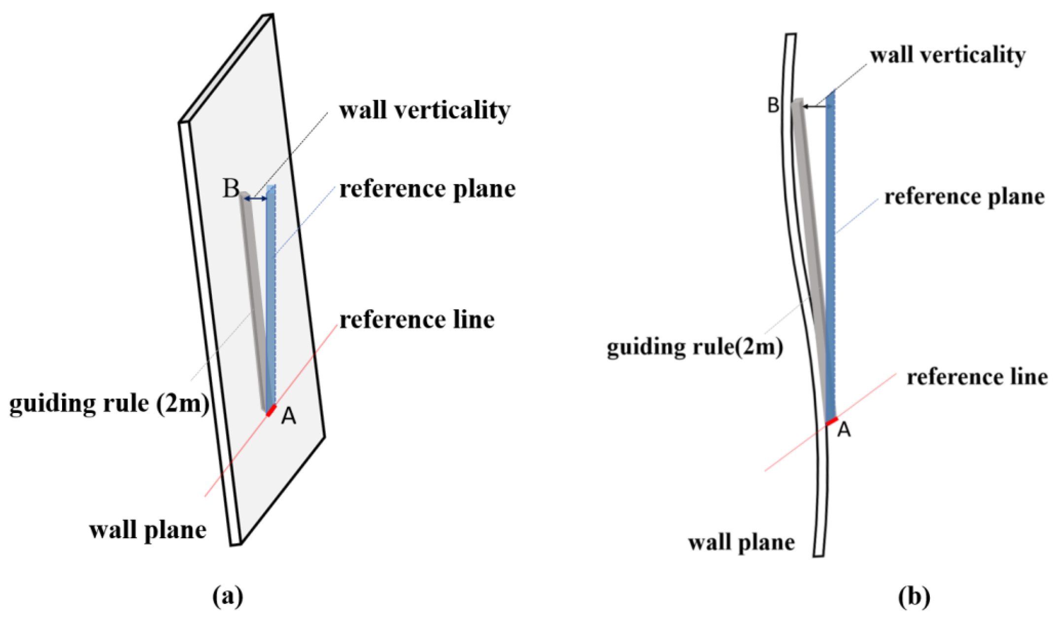
The verticality of the wall is an essential index that reflects the verticality and quality of the wall plane within the range of story height. According to the Chinese National Code for Acceptance of Construction Quality of Concrete Structures [1] and relevant enterprise standards, the verticality deviation of cast-in-place concrete structure dimensions is 5 mm (for walls height ≤ 6 m). The primary method of measurement is manual, and manual measurement mainly involves the following steps: when a 2 m ruler is vertically aligned with the measurement area, use one end of the guiding ruler (as illustrated in Zone A in Figure 10a) as the starting line to establish an upward plane (or downward when the top of the guiding ruler is vertically attached to the ceiling). The generated plane is used as the reference plane, and the maximum distance between the reference plane and the measurement area (such as the distance from area B to the blue reference plane in Figure 10b) is reflected on the dial of the measuring guiding rule, which is the key of verticality measurement. Therefore, this study simulates the measurement process in the manual process.
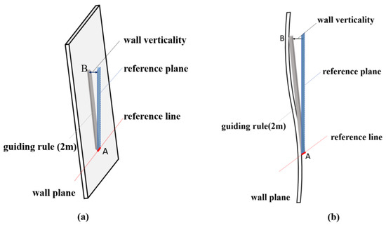
Figure 10.
The verticality calculation principle: (a) manual verticality measurement; (b) verticality measurement: reference plane and measurement area.
In the same way as in Section 3.2.1, the algorithm traverses each wall plane and identifies whether the plane is along the X-axis or Y-axis according to the coordinate extension orientation of the plane points. After the orientation is determined, the target wall is classified according to the measurement area. According to the measurement specification, it is necessary to complete three measurements on a wall when the length of the wall is longer than 3 m. It is measured once at the position 300 mm away from the internal and external corners of one side of the wall when the top of the guiding rule contacts the upper roof, it is measured once at the position 300 mm away from the internal and external corners of the other side of the wall when the bottom of the guiding rule contacts the lower ground, and the last measurement is performed in the middle of the wall. To make the measurement results more comprehensive, the length constraint of the wall is not considered, and three measurements on the measurable area of each wall are completed. During the three measurements, the part of the guiding rule against the wall each time is marked, as shown in the green part in Figure 11a, which simulates the steps of the measurement area covered by the guiding rule. At the same time, the area at the bottom of the lower, middle, and upper marked areas is used as the reference area, and upward and downward reference planes are generated, as shown in the blue part in Figure 11a. Then, the distances between each point of the marked green part points and the blue reference plane are calculated, as shown in Figure 11b.
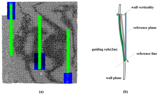
Figure 11.
The schematic diagram of the proposed algorithm (a) measurement simulation: guiding rule coverage and reference area; (b) distance calculation: green part points to blue reference plane.
As a wall is uninterrupted, the verticality is generally continuous and gradual rather than determined by a point. Therefore, the maximum distance from a point to the reference plane fails to be used as the basis for judging the verticality, and the color-coded measurement area is used to represent the verticality of the measurement area. As with the flatness threshold setting, the outward normal vector of the wall is used as the positive orientation to determine whether the measurement part is inclined backward or forward relative to the reference plane. For example, as shown in Figure 12a, the middle part of the measurement result is negative, and the maximum value area reaches 12 mm, which is marked in purple. The wall is inclined to the inside of the room and is detected as an unqualified area, which does not meet the requirements of the specification. The opposite is true if the calculation result is positive. In this study, each point is color-coded according to the positive and negative values of the distance deviation (note that the coding principle here is not the same as the flatness coding). The qualified standard value of reference verticality is 0 mm, 8 mm (plastering), and the value of the color interval is set to −12 mm, 12 mm. Each 2 mm between the areas is divided into a discontinuity so that the quality of each measurement area of the wall can be reflected comprehensively. The verticality situation of a wall can be viewed in three dimensions and can be arbitrarily rotated, enlarged, or shrunk, as shown in Figure 12a. Finally, the verticality color cloud map of each wall is reconstructed with relative orientations so that the verticality of the measurement parts of each room can be viewed in three dimensions, as shown in Figure 12b.

Figure 12.
The color cloud map of verticality: (a) wall verticality measurement result: negative deviation; (b) three-dimensional visualization of wall verticality color cloud map.
3.2.3. The Calculation and Visual Evaluation of the Door or Window Opening Dimension Index
During the process of traditional opening dimensions measurement, three measuring points are selected in the horizontal and vertical orientations for each frame, and the minimum measurement value in each orientation is used as the basis for dimension evaluation. In general, a ruler or laser rangefinder is used for measurement by one operator, and the other operator records the data on paper during the measurement. One end of the ruler (or rangefinder) is held against the measuring point, and the distance between the two ends is read after the ruler is stabilized. This section still simulates the measurement process in reality for the automated measurement of the index. The following part is the detailed measurement process of the opening dimensions.
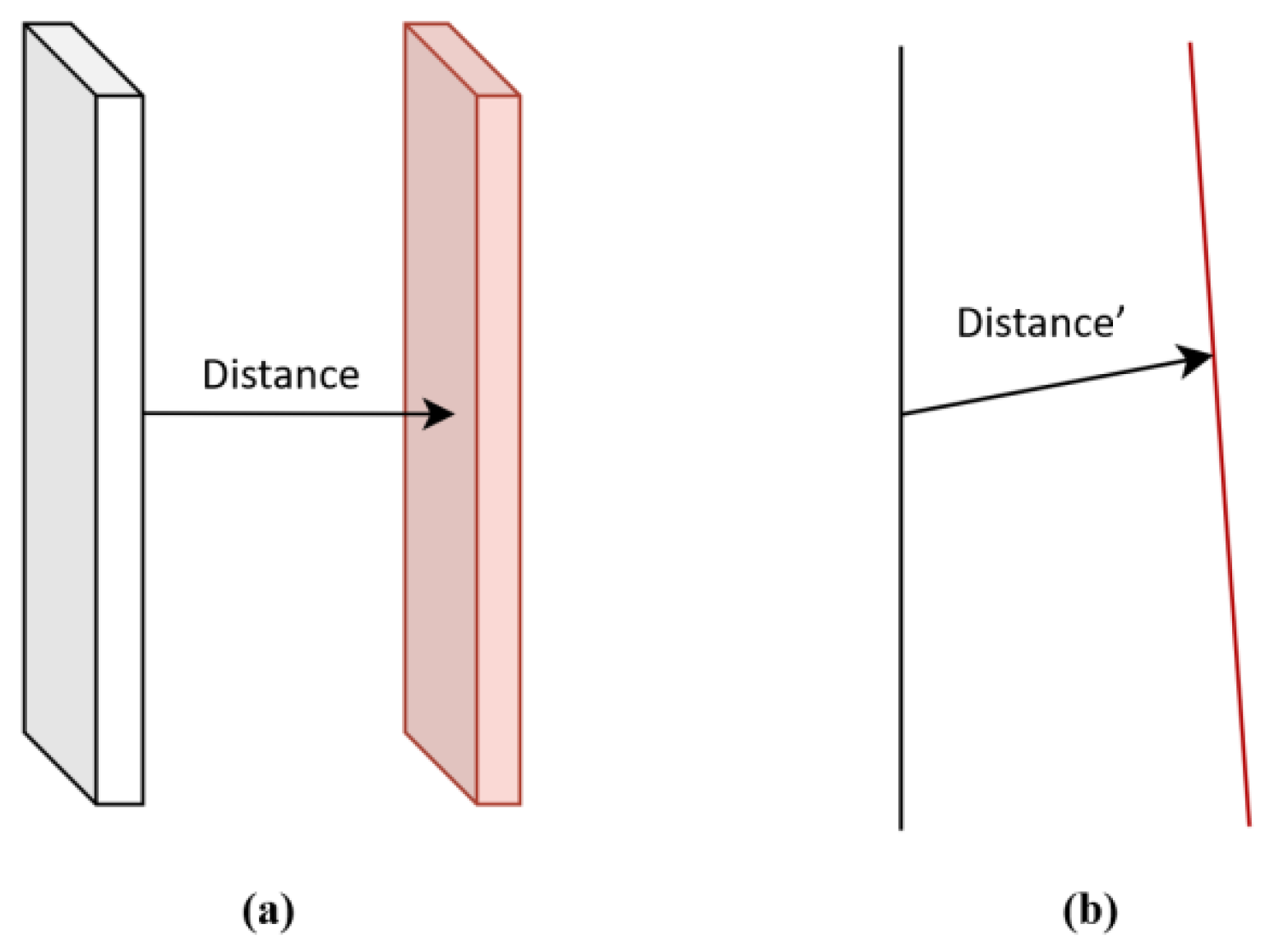
The measurement process of door or window opening dimensions in this section is shown in Figure 13. The proposed algorithm automatically identifies whether there are door or window opening clusters on the wall when traversing each wall and keeps traversing until the wall with door or window opening is fully accessed. Figure 14a shows the actual measurement principle. It is worth noting that the object wall may have vertical defects, which may affect the measurement of the opening dimensions if the door frame marked in pink on the right is inclined to the rear due to vertical defects. The scanned wall data are only one surface without thickness, which may result in Distance’ > Distance if the door frame marked pink is tilted backward, as shown in Figure 14b.

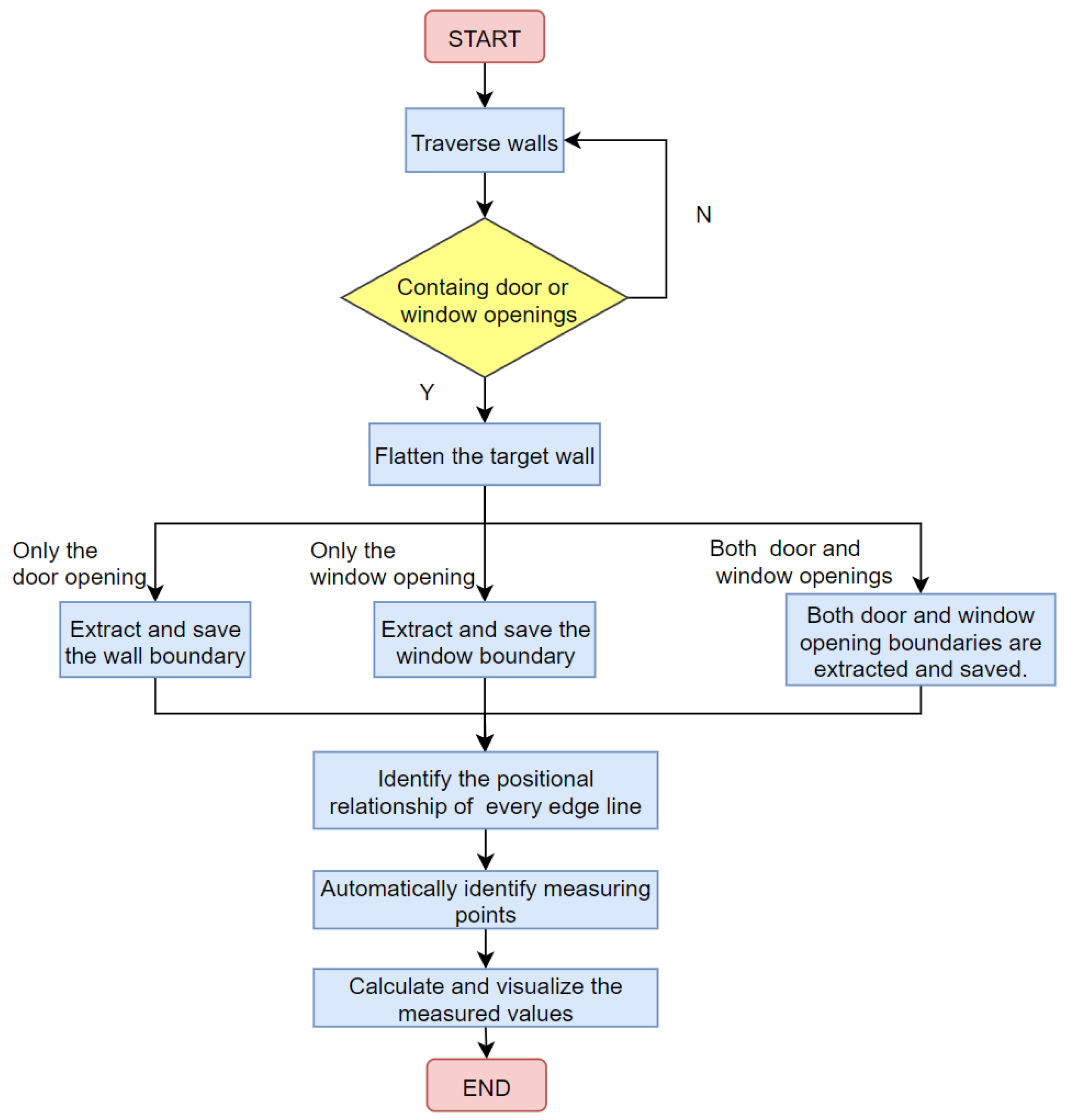
Figure 13.
The flow chart of the dimension calculation of door or window opening.
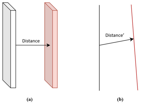
Figure 14.
The schematic diagram of opening dimension measurement in practice, (a) measurement principle: identification of door or window opening clusters, (b) potential impact of verticality defects on opening dimensions measurement.
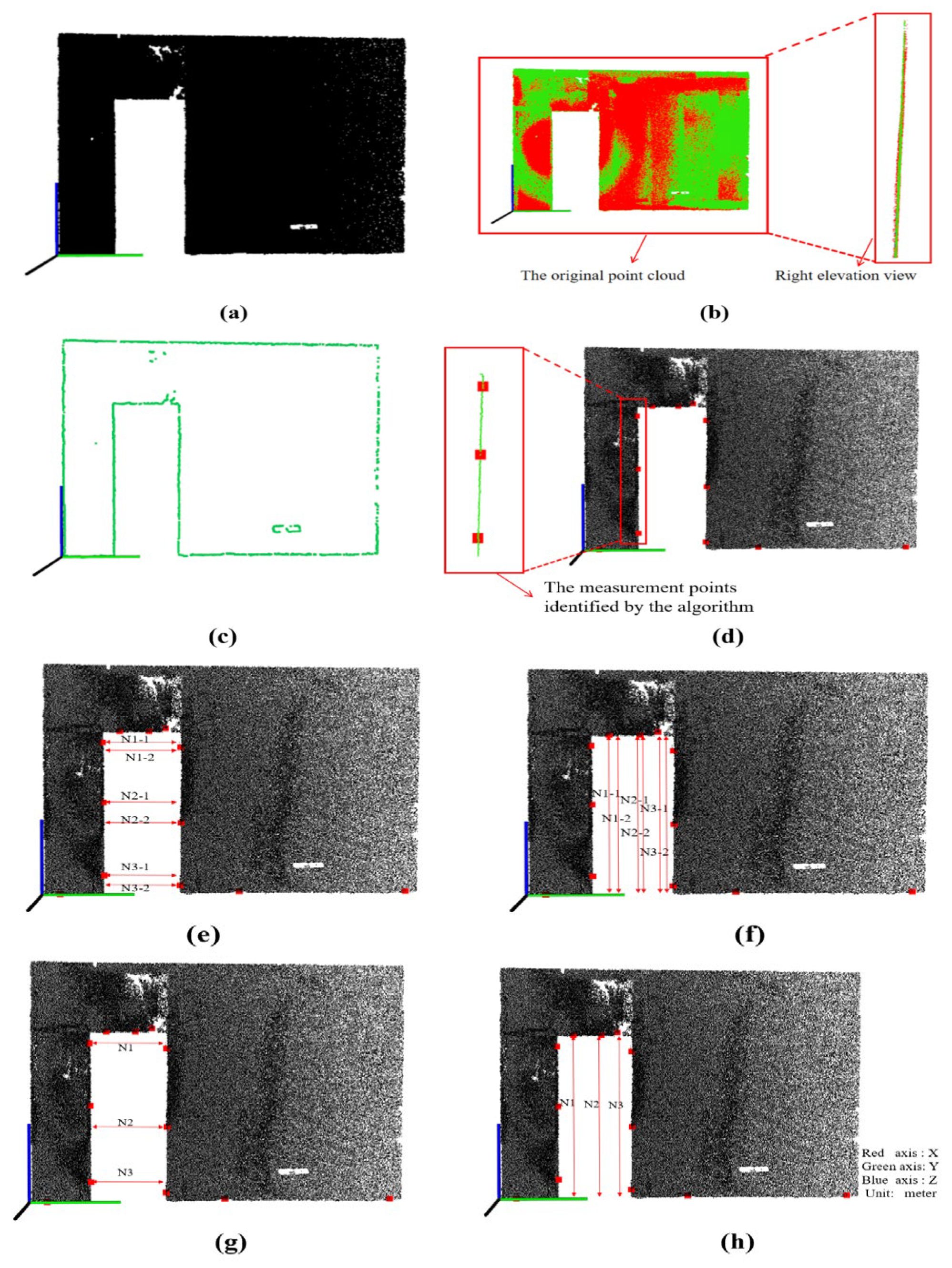
Therefore, the wall with a door or window opening is obtained through traversal, as shown in Figure 15a. The algorithm flattens the target wall as follows: Firstly, the target wall is fitted by means of the RANSAC algorithm. The proposed fitting does not need to identify a best fitting plane like the flatness fitting step in Section 3.2.1, and instead, it only needs to identify a projection plane with the same orientation. The fitting does not change the original data. The original point cloud still exists but generates a plane approximately coincident with the wall. Next, the fitting plane is used as the projection reference plane to project the target point cloud onto the plane. The red point plane is the origin point cloud, the green point plane is the flattened point cloud, and the right elevation view of the flattened wall data is shown in Figure 15b. This step does not change the geometric features of the opening dimensions measurement.

Figure 15.
The measurement process of the opening dimensions: (a) wall traversal with door or window opening; (b) flattened wall data right elevation view; (c) wall boundaries extraction door opening; (d) automatic detection points on door frame; (e) measurement values (N value1) for detection points; (f) measurement values (N value2) for detection points; (g) left view width of detection points; (h) right view width of detection points.
To reduce the influence of unnecessary points on the calculation, the algorithm extracts the overall boundary of the point cloud using normal vector estimation and K-d tree. It is worth mentioning that experiments show that the result based on the flattened wall point cloud for boundary extraction is more comprehensive. For the wall clusters with only door openings, the wall boundaries are extracted directly, as shown in Figure 15c. Then, three corresponding detection points are automatically extracted from the detection area on each door frame by the developed algorithm, as shown in Figure 15d. The distance from the detection point to the opposite frame line is calculated for the detection points on the left and right door frame, and the distance from the detection point to the intersecting line on the ground is calculated for the detection points on the upper border. The two measurement values in the same measuring area are, respectively, denoted as N value-1 and N value-2, as shown in Figure 15e,f, and the average value of the two measurement values is calculated as , which is used as a final measurement value. Finally, the detection distance value of each detection point is displayed in the 3D visualization window, which includes a left and right view window. The left view shows the width of all detection points (Figure 15g), the right view shows the height of all detection points (Figure 15h), and the N value corresponds to the detection value of the detection point. After the calculation, the measurement results of the door and window openings on the wall can be viewed in 3D, freely rotated, and zoomed in or zoomed out to see the measured values more clearly.
4. Case Study
To validate the proposed indoor geometric quality inspection method, a construction site located in Shenzhen, Guangdong Province, China, was selected as an example in May 2023. A group of residential rooms, including the living room, master bedroom, guest room, and baby room, were chosen for validation. The point cloud data of the object rooms were processed using the proposed method. After the data were calculated and analyzed, the results calculated via the proposed method were compared and analyzed with manual measurement data to verify the accuracy of the proposed method. The whole process was run on a high-performance computer with Intel Core i7-10875H CPU and 32 GB RAM, and all the algorithms were developed in C++. The data acquisition method and detailed analysis of the data are discussed in the following sections.
4.1. Data Acquisition
In this experiment, the point cloud data of a residence were acquired from the completed rooms using a Trimble X7 laser scanner (Figure 16a) with an accuracy of 2.4 mm–6.0 mm in a range of 10 m–40 m, which is suitable for room space point cloud data collection and can meet the accuracy requirements of indoor geometric quality detection. The scanner is equipped with the state-of-the-art Trimble X-Drive alignment system, enabling automatic calibration. Additionally, prior to scanning, it employs corresponding station planning algorithms to ensure the accuracy of scanner positioning at each scanning location. This ensures that the scanning data are automatically registered, facilitating seamless data collection without the need for concerns about site alignment. After the data were calculated and analyzed by the proposed method, the guiding ruler (Figure 16a) was used to obtain manual measurement data of wall flatness and verticality. A Xiaomi intelligent laser rangefinder (Figure 16a), which can measure in real time with an accuracy of 3 mm in a range of 40 m, was used to manually measure the opening dimensions. There was little clutter in the selected scene, so the scanned data were relatively clean. For the scan work, one base station was installed in each room, and an additional base station was installed in the corridor for connection. It took 3–4 min to scan a station. The entire scan work took 21 min, including 459,164,358 points, and the original scanned data are shown in Figure 16b.
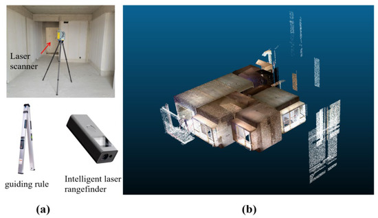
Figure 16.
Tools and scene of the scan work: (a) three tools used for this scan and (b) the original point cloud of the scan.
4.2. Results and Discussion
The simple manual segmentation operation and the assistance of the DBSCAN algorithm quickly remove the outliers that do not belong to the residence and obtain most of the valid data. The processing result is shown in Figure 17a. The amount of collected original data is large, and the coordinate system of the original data is uncertain, which is not suitable for the calculation and analysis of the data. Hence, each room was separated individually with a simple manual split using CloudCompare, as shown in Figure 17b. Each room, which can be imported directly into the system of the proposed method, mainly included four walls and window or door openings. Next, the coordinate transformation algorithm was separately performed for each room, as shown in Figure 18. The number of points in the whole residence was reduced from 459,164,358 to 12,834,623 through the VGD down-sampling algorithm. However, there may still be noisy points in the rooms. The statistical outlier removal denoising algorithm was used to remove obvious outliers, which were sparsely distributed in each room. Then, the developed Cube Diagonal-based Denoising algorithm, which could remove the outliers attached to walls, floors, and ceilings at close range, was used to finish the fine denoising. Figure 19 shows the effect of the two denoising processes, where the red part represents the area denoised twice, and the green part represents the removed noise. After the ceiling and floor were extracted, the scanned wall point of each room was segmented into four separate walls through the improved normal-region growing algorithm, as shown in Figure 20.
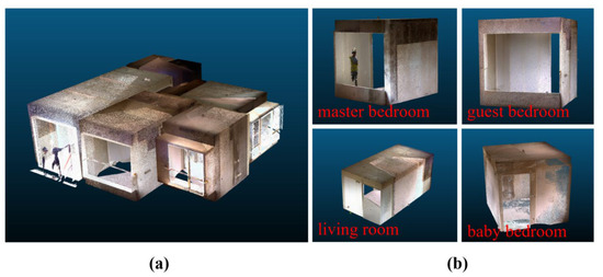
Figure 17.
Point cloud data for preliminary processing: (a) point cloud data for preliminary cluster denoising and (b) point cloud data for preliminary segmentation.

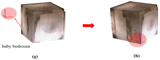
Figure 18.
Coordinate transformation of different rooms, (a,b) living room coordinate transformation process, (c,d) master bedroom coordinate transformation process, (e,f) guest bedroom coordinate transformation process, (g,h) baby bedroom coordinate transformation process.
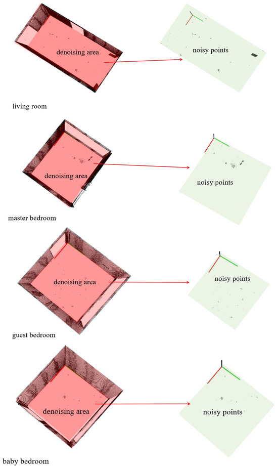
Figure 19.
Coarse denoising and fine denoising results in different rooms.
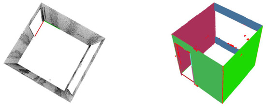
Figure 20.
Wall segmentation through the improved normal-region growing algorithm.
The calculation of each measured index could be completed when the ceiling, floor, and four walls of a room were identified separately by means of the proposed method. The wall point clouds were used to calculate the flatness, verticality, and dimensions of the openings. In order to obtain a more comprehensive view of the index calculation results of the whole room, the coordinate transformation parameters for all individual rooms were automatically identified to complete the coordinate system restoration. Then, the algorithm calculated the related measurement value of each point in each involved area and presented the results on points to provide an intuitive, real, and all-around visualization of the results. Figure 21a,b, respectively, show the color-coded cloud map of flatness and verticality deviation, and workers could identify defects according to the color of wall parts to guide later repair work. Figure 21c,d, respectively, show the width and height dimensions of all room openings, and workers could compare the dimensions of the openings in the corresponding orientation on the drawing with the measurement in the 3D view to verify that the dimensions conform to the specification. Figure 21 shows a collection of all the calculated results for all the measured indexes in all the rooms.
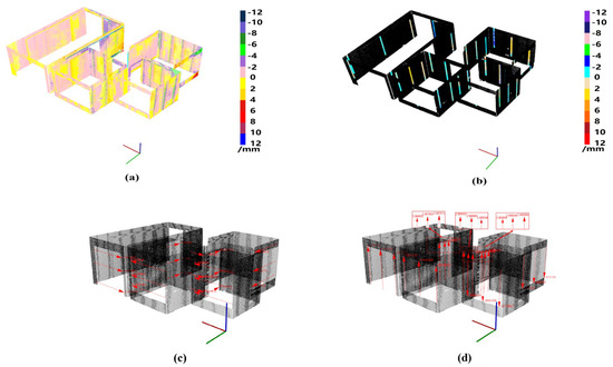
Figure 21.
Visualization of the calculation and analysis results of the indoor geometric quality: (a) color-coded cloud map of flatness deviation, (b) color-coded cloud map of vertical deviation, (c) dimensional visualization of opening width, and (d) dimensional visualization of opening height.
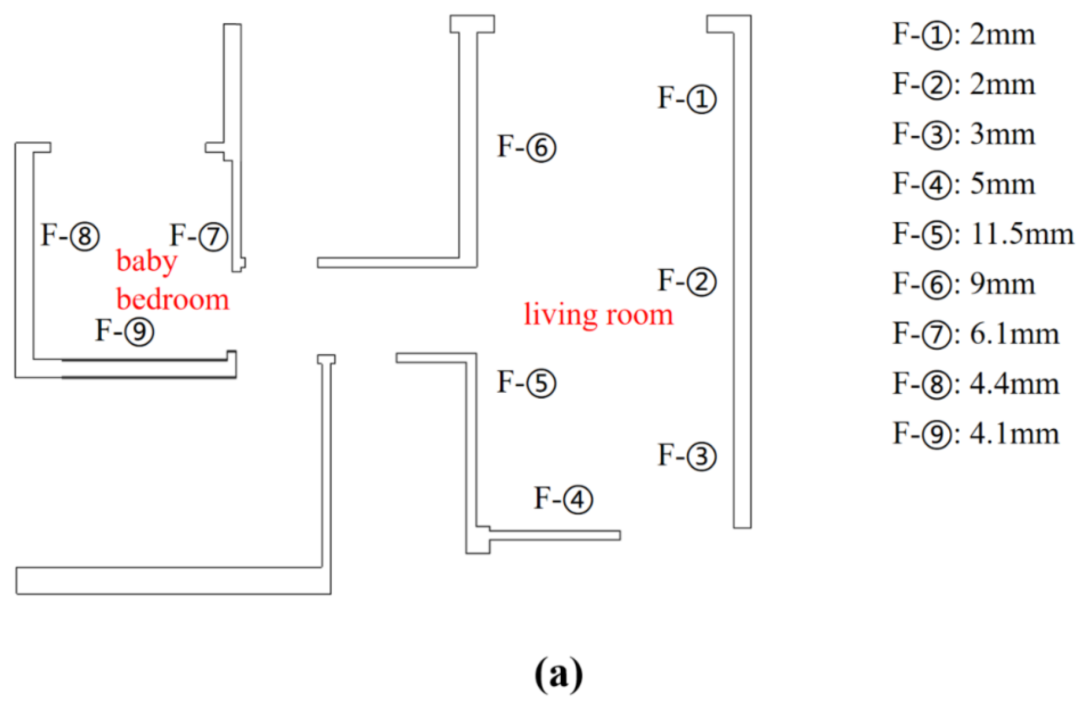
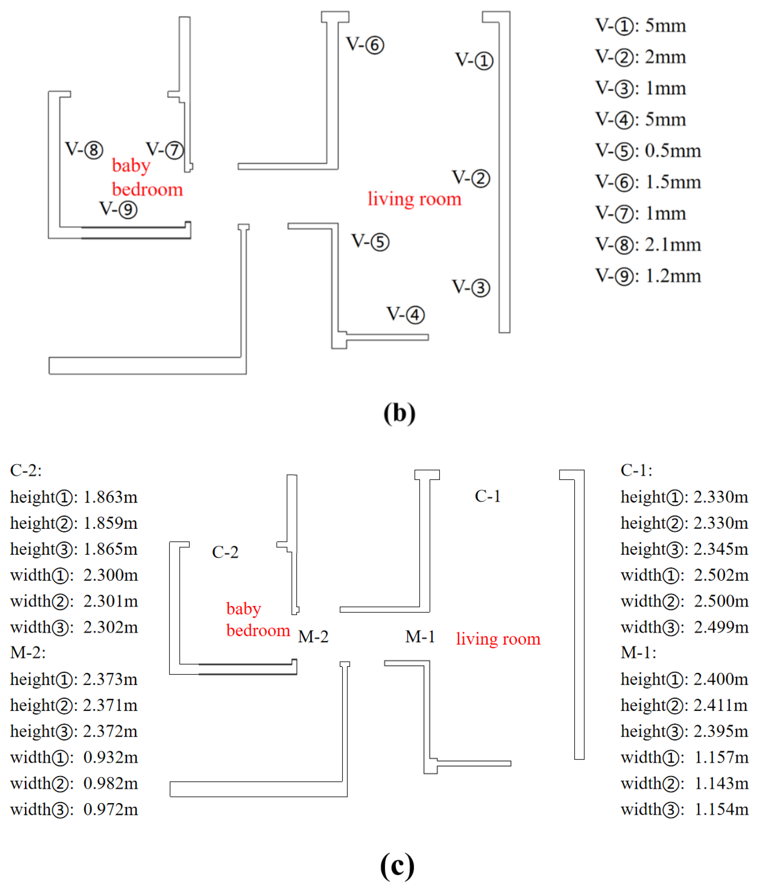
According to the specification [1], the plane flatness, verticality, and opening dimension tolerances of cast-in-place concrete should be 8 mm, 10 mm, and 20 mm, respectively. In order to verify the effectiveness of the proposed method, manual measurements were finished on site (Figure 22). Then, the living room and baby bedroom data were selected for the accuracy monitoring of the proposed method, and the measurement positions were marked in advance to ensure the consistency of the measurement positions. Figure 23 shows the results of manual measurements performed by the researchers in the living room and baby bedroom. The F-value and V-value, respectively, represent the manual measurement values of the flatness and verticality of walls at the corresponding position, and height ①, height ②, and height ③ and width ①, width ②, and width ③, respectively, represent three measurements of the corresponding height and width on the border of different openings. Figure 24 shows the proposed method’s measurement results for the selected rooms, and the manual measurement data are compared with the proposed method in Table 1.
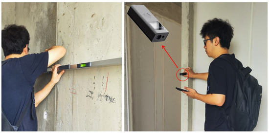
Figure 22.
Manual measurements on the construction site.
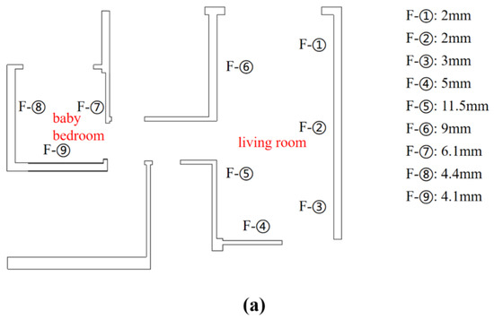
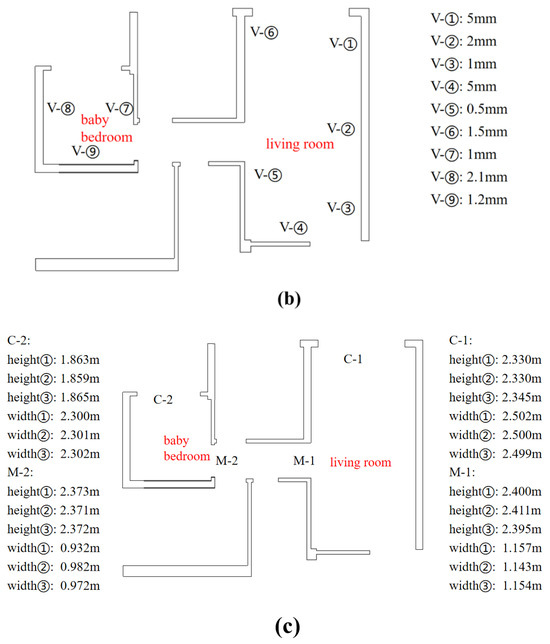
Figure 23.
Manual measurement results of the selected rooms: (a) flatness measurement results, (b) verticality measurement results, and (c) opening dimension measurement results.
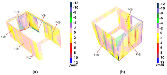
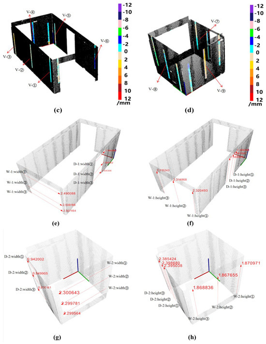
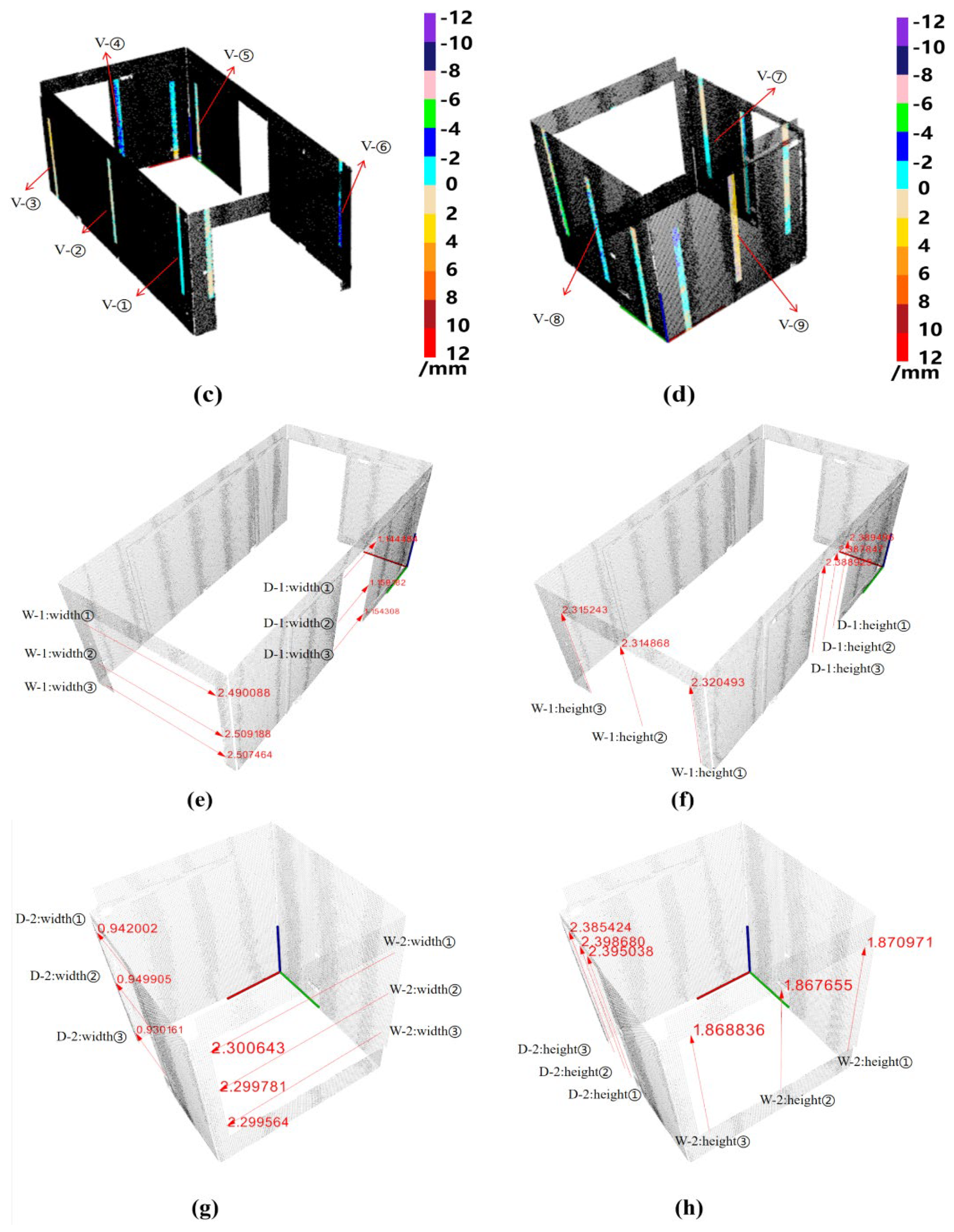
Figure 24.
The proposed method measurement results of the selected rooms: (a,b) flatness measurement results, (c,d) verticality measurement results, (e,f) measurement results of opening dimensions in living room, and (g,h) measurement results of opening dimensions in baby bedroom.

Table 1.
The compared results of manual measurement and the proposed method: (a) verification of flatness and verticality measurement results, (b) verification of measurement results of window openings, and (c) verification of measurement results of door openings.
It is worth noting that when the plane is fitted using RANSAC, the position of the original wall will be slightly affected, which causes the measured value of the proposed method to deviate slightly from the actual value by 0–1 mm. Due to the possible inconsistency of the measurement position, the subjective factors of manual measurement, and the flatness of the opening frame, the flatness, the verticality error value of 0–3 mm, and the opening dimension error value of 0–0.01 m are regarded as the effective values. As shown in Table 1a, there are nine measuring parts in the two rooms. Both manual measurement and the proposed method show that the flatness values of F-⑤ and F-⑥ are not in accordance with the specification, and all the measured verticality values are in accordance with the specification. In the F-⑤ and F-⑦ measurement areas, the error values between manual measurement and the proposed method are relatively large, at 1–3.5 mm and 4.1–6.1 mm, respectively, and are regarded as ineffective values. In other areas, the error values are all between 0 and 3 mm, which are regarded as effective values. In the V-① measurement area, the error value is 3–5 mm, which is regarded as an ineffective value. As shown in Table 1b,c, the measurement error of width ② of D-2 is 0.010 m, which is regarded as an ineffective value, and all dimensional measurements in the remaining area are valid.
Table 2 presents the time consumption of the measurement method proposed in this paper compared to the current basic measurement method (manual measurement). The time consumption for the proposed method includes four components: (1) site planning and the scanning and preprocessing of point cloud data, (2) the flatness measurement time, (3) the verticality calculation time, and (4) the opening size calculation time. The proposed method takes a total of 28.5 min. In comparison to the commonly used measurement method, this method saves 27.5 min, accounting for 49.11% of the total measurement time. The calculation time of the proposed method varied with the density of point cloud data. Hence, the point cloud density can be appropriately reduced to improve computing efficiency. In summary, the accuracy of the proposed method was 77.8% for flatness, 88.9% for verticality, and 95.9% for opening dimensions. At the same time, a Mann–Whitney U test was conducted to compare the results of manual measurements with the measurements obtained using the proposed method. The significance of the test showed no significant difference, indicating that there is no substantial difference between manual measurements and laser measurements. Therefore, the measurement results of the proposed method are consistent with manual measurements, demonstrating that the proposed method can effectively replace manual work in order to efficiently and accurately measure the flatness and verticality of walls and the dimensions of door and window openings.
Table 2.
Time-statistical comparison between the measurement method proposed in this paper and the basic measurement method.
Based on the experimental results in Section 4.2, the feasibility of the indoor geometric measurement method based on 3D laser scanning is demonstrated. This method, through steps such as coordinate transformation, data denoising, and semantic segmentation, can rapidly obtain accurate measurement results. According to on-site experimental results, when compared to manual measurements, this method achieved a planarity accuracy of 77.8%, verticality accuracy of 88.9%, and opening size accuracy of 95.9%. The overall time required was significantly reduced, with a 49.11% reduction in time consumption in this experiment. The introduction of automated color-coded maps and visualizations of opening sizes provides intuitive feedback on flatness and opening dimensions, enabling construction personnel to promptly identify problematic areas. Furthermore, when comparing the proposed method with traditional measurement methods, it is evident that the measurement results meet the requirements, and measurement efficiency is significantly improved.
However, it is worth noting that when using RANSAC for plane fitting, this method may slightly affect the original wall positions, resulting in some discrepancies between measured values and actual values. Although these discrepancies are relatively small, in some cases, further calibration may be necessary to ensure measurement accuracy. Additionally, the proposed method still has some limitations. For example, it is primarily applicable to rectangular residential buildings, and optimization is required for non-rectangular structures. Moreover, certain manual tasks are still part of the data processing phase.
5. Conclusions and Future Work
This study introduces an automated non-contact indoor geometric quality measurement method based on ground laser scanning. It is used for measuring and visualizing the flatness and verticality of indoor walls, as well as the dimensions of door and window openings. The method involves steps such as point cloud data collection, coordinate transformation, data denoising, semantic segmentation, reassembly, and plane traversal for geometric quality calculation and visualization. The method is applied to data collection and experimental verification in the residential building handover phase, and it is compared with common measurement methods. Experimental results show that this method offers high accuracy, high measurement efficiency, and reduces measurement time by half.
In this study, laser scanning is combined with various measurement techniques to propose a semi-automatic point cloud coordinate transformation method. Building upon this, the Cube Diagonal-based Denoising algorithm is introduced for fine point cloud denoising, effectively eliminating noise attached to the room interior and surfaces. Additionally, the use of intuitive color-coded point cloud maps for flatness and verticality measurements enables precise defect recognition. For opening sizes, a digital visualization method is employed, providing an intuitive display of the dimensions of all openings within residential spaces. This method serves as an improved alternative to traditional measurement techniques, guiding personnel in identifying and locating dimension defects.
However, some data processing tasks still require manual or semi-automatic handling, and future research should focus on fully automatic room segmentation methods for more efficient segmentation. Furthermore, as the methods developed in this study are implemented in C++, they can be embedded in mobile devices or robots to create more flexible and efficient indoor geometric quality inspection systems. Additionally, visual results can be combined with technologies like augmented reality (AR) to offer more intuitive guidance for rectifying non-compliant work.
Author Contributions
Conceptualization, Y.T.; Methodology, Y.T. and S.J.; Software, X.L., S.J. and Q.W.; Validation, S.J.; Formal analysis, Y.T.; Data curation, Y.T. and X.L.; Writing—original draft, Y.T., X.L. and S.J.; Writing—review & editing, Y.T., X.L. and Q.W.; Visualization, Q.W.; Supervision, Y.T., D.W. and X.X.; Project administration, Y.T., Q.W., D.W. and X.X.; Funding acquisition, Y.T. All authors have read and agreed to the published version of the manuscript.
Funding
This research is supported by the Natural Science Foundation of Guangdong Province of China (No. 2023A1515011119), the Young Scientists Fund of the National Natural Science Foundation of China (No. 52308319), and Shenzhen University 2035 Program for Excellent Research (2022B007).
Data Availability Statement
Some of the data, models, or code that support the findings of this study are available from the corresponding author upon reasonable request.
Conflicts of Interest
Daochu Wang and Xiaofeng Xie were employed by Guangzhou Construction Engineering Co., Ltd. The remaining authors declare that the research was conducted in the absence of any commercial or financial relationships that could be construed as a potential conflicts of interest.
References
- GB50204-201; Code for Acceptance of Construction Quality of Concrete Structures. China Building Industry Press: Beijing, China, 2015.
- Li, D.; Liu, J.; Feng, L.; Zhou, Y.; Liu, P.; Chen, Y.F. Terrestrial laser scanning assisted flatness quality assessment for two different types of concrete surfaces. Measurement 2020, 154, 107436. [Google Scholar] [CrossRef]
- Bosché, F.; Biotteau, B. Terrestrial laser scanning and continuous wavelet transform for controlling surface flatness in construction—A first investigation. Adv. Eng. Inform. 2015, 29, 591–601. [Google Scholar] [CrossRef]
- Tang, P.; Huber, D.; Akinci, B. Characterization of laser scanners and algorithms for detecting flatness defects on concrete surfaces. J. Comput. Civ. Eng. 2011, 25, 31–42. [Google Scholar] [CrossRef]
- Ballast, D.K. Handbook of Construction Tolerances; John Wiley & Sons: Hoboken, NJ, USA, 2007. [Google Scholar]
- Wang, Q.; Kim, M.-K.; Sohn, H.; Cheng, J.C. Surface flatness and distortion inspection of precast concrete elements using laser scanning technology. Smart Struct. Syst 2016, 18, 601–623. [Google Scholar] [CrossRef]
- Cao, Y.; Liu, J.; Feng, S.; Li, D.; Zhang, S.; Qi, H.; Cheng, G.; Chen, Y.F. Towards automatic flatness quality assessment for building indoor acceptance via terrestrial laser scanning. Measurement 2022, 203, 111862. [Google Scholar] [CrossRef]
- BS 8204-1:2003+A1:2009; Screeds, Bases and In situ Flooring. British Standards Institution: London, UK, 2009.
- BS EN 13670:2009; Execution of Concrete Structures. British Standards Institution: London, UK, 2009.
- Group, T.C.S. National Structural Concrete Specification for Building Construction, 4th ed.; The Concrete Structures Group: London, UK, 2010. [Google Scholar]
- Cheok, G.S.; Stone, W.C.; Lipman, R.R.; Witzgall, C. Lipman, and Christoph Witzgall. Ladars for construction assessment and update. Autom. Constr. 2000, 9, 463–477. [Google Scholar] [CrossRef]
- Akinci, B.; Boukamp, F.; Gordon, C.; Huber, D.; Lyons, C.; Park, K. A formalism for utilization of sensor systems and integrated project models for active construction quality control. Autom. Constr. 2006, 15, 124–138. [Google Scholar] [CrossRef]
- Bosche, F.; Haas, C.T.; Akinci, B. Automated recognition of 3D CAD objects in site laser scans for project 3D status visualization and performance control. ASCE J. Comput.Civ. Eng 2009, 23, 311–318. [Google Scholar] [CrossRef]
- Opfer, N.D. Construction Defect Education in Construction Management; California Polytechnic University: San Luis Obispo, CA, USA, 1999. [Google Scholar]
- Kim, M.-K.; Sohn, H.; Chang, C.-C. Localization and Quantification of Concrete Spalling Defects Using Terrestrial Laser Scanning. J. Comput. Civ. Eng. 2015, 29, 04014086. [Google Scholar] [CrossRef]
- Kim, M.-K.; Wang, Q.; Li, H. Non-contact sensing based geometric quality assessment of buildings and civil structures: A review. Autom. Constr. 2019, 100, 163–179. [Google Scholar] [CrossRef]
- Wu, Z.; Song, S.; Khosla, A.; Yu, F.; Zhang, L.; Tang, X.; Xiao, J. 3d shapenets: A deep representation for volumetric shapes. In Proceedings of the IEEE Conference on Computer Vision and Pattern Recognition, Boston, MA, USA, 7–12 June 2015; pp. 1912–1920. [Google Scholar] [CrossRef]
- Qi, C.R.; Yi, L.; Su, H.; Guibas, L.J. Pointnet: Deep learning on point sets for 3d classification and segmentation. arXiv 2016, arXiv:1612.00593. [Google Scholar] [CrossRef]
- Qi, C.R.; Yi, L.; Su, H.; Guibas, L.J. Pointnet++: Deep hierarchical feature learning on point sets in a metric space. arXiv 2017, arXiv:1706.02413. [Google Scholar] [CrossRef]
- Yang, G.; Huang, X.; Hao, Z.; Liu, M.-Y.; Belongie, S.; Hariharan, B. Pointflow: 3d point cloud generation with continuous normalizing flows. arXiv 2019, arXiv:1906.12320. [Google Scholar] [CrossRef]
- Zamorski, M.; Zięba, M.; Klukowski, P.; Nowak, R.; Kurach, K.; Stokowiec, W.; Trzciński, T.S.; Trzcinski, T. Adversarial autoencoders for compact representations of 3d point clouds. arXiv 2018, arXiv:1811.07605. [Google Scholar] [CrossRef]
- Spurek, P.; Winczowski, S.; Tabor, J.; Zamorski, M.; Zieba, M.; Trzciński, T. Hypernetwork approach to generating point clouds. In Proceedings of the 37th International Conference on Machine Learning (ICML), Virtual Event, 13–18 July 2020. [Google Scholar] [CrossRef]
- Tang, P.; Huber, D.; Akinci, B.; Lipman, R.; Lytle, A. Automatic reconstruction of as-built building information models from laser-scanned point clouds: A review of related techniques. Autom. Constr. 2010, 19, 829–843. [Google Scholar] [CrossRef]
- Lu, Q.; Lee, S. Image-based technologies for constructing as-is building information models for existing buildings. J. Comput. Civ. Eng. 2017, 31, 04017005. [Google Scholar] [CrossRef]
- Olsen, M.J.; Kuester, F.; Chang, B.J.; Hutchinson, T.C. Terrestrial laser scanning-based structural damage assessment. J. Comput. Civ. Eng. 2009, 24, 264–272. [Google Scholar] [CrossRef]
- Zalama, E.; Gómez-García-Bermejo, J.; Llamas, J.; Medina, R. An effective texture mapping approach for 3D models obtained from laser scanner data to building documentation. Comput.-Aided Civ. Infrastruct. Eng. 2011, 26, 381–392. [Google Scholar] [CrossRef]
- Olsen, M.J. In Situ Change Analysis and Monitoring through Terrestrial Laser Scanning. J. Comput. Civ. Eng. 2015, 29, 04014040. [Google Scholar] [CrossRef]
- Hansen, E.H.; Gobakken, T.; Næsset, E. Effects of pulse density on digital terrain models and canopy metrics using airborne laser scanning in a tropical rainforest. Remote Sens. 2015, 7, 8453–8468. [Google Scholar] [CrossRef]
- Brilakis, I.; Fathi, H.; Rashidi, A. Progressive 3D reconstruction of infrastructure with videogrammetry. Autom. Constr. 2011, 20, 884–895. [Google Scholar] [CrossRef]
- Wang, Q.; Tan, Y.; Mei, Z. Computational Methods of Acquisition and Processing of 3D Point Cloud Data for Construction Applications. Arch. Comput. Methods Eng. 2019, 27, 479–499. [Google Scholar] [CrossRef]
- Xu, Z.; Kang, R.; Lu, R. 3D Reconstruction and Measurement of Surface Defects in Prefabricated Elements Using Point Clouds. J. Comput. Civ. Eng. 2020, 34 Pt 8, 04020033. [Google Scholar] [CrossRef]
- Wang, Q.; Kim, M.-K. Applications of 3D point cloud data in the construction industry: A fifteen-year review from 2004 to 2018. Adv. Eng. Inform. 2019, 39, 306–319. [Google Scholar] [CrossRef]
- Fröhlich, C.; Mettenleiter, M. Terrestrial laser scanning—New perspectives in 3D surveying. Int. Arch. Photogramm. Remote Sens. 2004, 36, W2. [Google Scholar]
- Zhang, C.; Arditi, D. Automated progress control using laser scanning technology. Autom. Constr. 2013, 36, 108–116. [Google Scholar] [CrossRef]
- Boukamp, F.; Akinci, B. Automated processing of construction specifications to support inspection and quality control. Autom. Constr. 2007, 17, 90–106. [Google Scholar] [CrossRef]
- Stypułkowski, M.; Kania, K.; Zamorski, M.; Zięba, M.; Trzciński, T.; Chorowski, J. Representing point clouds with generative conditional invertible flow networks. Pattern Recognit. Lett. 2021, 150, 26–32. [Google Scholar] [CrossRef]
- Xiang, C.; Qi, C.R.; Li, B. Generating 3d adversarial point clouds. arXiv 2018, arXiv:1809.07016. [Google Scholar] [CrossRef]
- Yue, X.; Wu, B.; Seshia, S.A.; Keutzer, K.; Sangiovanni-Vincentelli, A.L. A lidar point cloud generator: From a virtual world to autonomous driving. In Proceedings of the 2018 ACM on International Conference on Multimedia Retrieval, Yokohama, Japan, 11–14 June 2018. [Google Scholar] [CrossRef]
- Bosché, F.; Guenet, E. Automating surface flatness control using terrestrial laser scanning and building information models. Autom. Constr. 2014, 44, 212–226. [Google Scholar] [CrossRef]
- ACI. ACI 302.1R-96—Guide for Concrete Floor and Slab Construction; ACI: Farmington Hills, MI, USA, 1997. [Google Scholar] [CrossRef]
- Kim, M.-K.; Wang, Q.; Park, J.-W.; Cheng, J.C.P.; Sohn, H.; Chang, C.-C. Automated dimensional quality assurance of full-scale precast concrete elements using laser scanning and BIM. Autom. Constr. 2016, 72, 102–114. [Google Scholar] [CrossRef]
- Boehler, W.; Heinz, G.; Marbs, A. The potential of non-contact close range laser scanners for cultural heritage recording. Int. Arch. Photogramm. Remote Sens. Spat. Inf. Sci. 2002, 34, 430–436. [Google Scholar] [CrossRef]
- Yastikli, N. Documentation of cultural heritage using digital photogrammetry and laser scanning. J. Cult. Herit. 2007, 8, 423–427. [Google Scholar] [CrossRef]
- Du, J.-C.; Teng, H.-C. 3D laser scanning and GPS technology for landslide earthwork volume estimation. Autom. Constr. 2007, 16, 657–663. [Google Scholar] [CrossRef]
- Jaselskis, E.J.; Gao, Z.; Walters, R.C. Improving transportation projects using laser scanning. J. Constr. Eng. Manag. 2005, 131, 377–384. [Google Scholar] [CrossRef]
- Priestnall, G.; Jaafar, J.; Duncan, A. Extracting urban features from LiDAR digital surface models. Comput. Environ. Urban Syst. 2000, 24, 65–78. [Google Scholar] [CrossRef]
- El-Omari, S.; Moselhi, O. Integrating 3D laser scanning and photogrammetry for progress measurement of construction work. Autom. Constr. 2008, 18, 1–9. [Google Scholar] [CrossRef]
- Turkan, Y.; Bosche, F.; Haas, C.T.; Haas, R. Automated progress tracking using 4D schedule and 3D sensing technologies. Autom. Constr. 2012, 22, 414–421. [Google Scholar] [CrossRef]
- Hutchinson, T.C.; Chen, Z. Improved image analysis for evaluating concrete damage. J. Comput. Civ. Eng. 2006, 31, 210–216. [Google Scholar] [CrossRef]
- Zhu, Z. Column Recognition and Defects/damage Properties Retrieval for Rapid Infrastructure Assessment and Rehabilitation using Machine Vision. Ph.D. Thesis, Georgia Institute of Technology, Atlanta, GA, USA, 2011. [Google Scholar]
- Dawood, T.; Zhu, Z.; Zayed, T. Machine vision-based model for spalling detection and quantification in subway networks. Autom. Constr. 2017, 81, 149–160. [Google Scholar] [CrossRef]
- Tang, D.; Li, S.; Wang, Q.; Li, S.; Cai, R.; Tan, Y. Automated Evaluation of Indoor Dimensional Tolerance Compliance Using the TLS Data and BIM; Springer Books: Berlin/Heidelberg, Germany, 2021. [Google Scholar] [CrossRef]
- Tang, S.; Golparvar-Fard, M.; Naphade, M.; Gopalakrishna, M.M. Video-Based Motion Trajectory Forecasting Method for Proactive Construction Safety Monitoring Systems. J. Comput. Civ. Eng. 2020, 34, 0402004. [Google Scholar] [CrossRef]
- Tan, Y.; Chen, L.; Wang, Q.; Li, S.; Deng, T.; Tang, D. Geometric Quality Assessment of Prefabricated Steel Box Girder Components Using 3D Laser Scanning and Building Information Model. Remote Sens. 2023, 15, 556. [Google Scholar] [CrossRef]
- ACI. ACI 117-06—Specifications for Tolerances for Concrete Construction and Materials and Commentary; American Concrete Institute: Farmington Hills, MI, USA, 2006. [Google Scholar]
- ASTM E 1155-96; Standard Test Method for DeterminingFF Floor Flatness andFLFloor Levelness Numbers. ASTM International: West Conshohocken, PA, USA, 2008. [CrossRef]
- Shih, N.-J.; Wang, P.-H. Using point cloud to inspect the construction quality of wall finish. Digit. Des. Educ. 2013, 573–578. [Google Scholar] [CrossRef]
- Tang, P.; Akinci, B.; Huber, D. Characterization of three algorithms for detecting surface flatness defects from dense point clouds. In IS&T/SPIE Conference on Electronic Imaging; Science Technology; SPIE: Washington, DC, USA, 2009; Volume 7239. [Google Scholar] [CrossRef]
- Bosché, F. Automated recognition of 3D CAD model objects in laser scans and calculation of as-built dimensions for dimensional compliance control in construction. Adv. Eng. Inform. 2010, 24, 107–118. [Google Scholar] [CrossRef]
- Zolanvari, S.M.I.; Laefer, D.F.; Natanzi, A.S. Three-dimensional building façade segmentation and opening area detection from point clouds. ISPRS J. Photogramm. Remote Sens. 2018, 143, 134–149. [Google Scholar] [CrossRef]
- Li, D.; Liu, J.; Hu, S.; Cheng, G.; Li, Y.; Cao, Y.; Dong, B.; Chen, Y.F. A deep learning-based indoor acceptance system for assessment on flatness and verticality quality of concrete surfaces. J. Build. Eng. 2022, 51, 104284. [Google Scholar] [CrossRef]
- Puri, N.; Valero, E.; Turkan, Y.; Bosché, F.; Bosché, F. Assessment of compliance of dimensional tolerances in concrete slabs using TLS data and the 2d continuous wavelet transform. Autom. Constr. 2018, 94, 62–72. [Google Scholar] [CrossRef]
- Kim, M.-K.; Sohn, H.; Chang, C.-C. Automated dimensional quality assessment of precast concrete panels using terrestrial laser scanning. Autom. Constr. 2014, 45, 163–177. [Google Scholar] [CrossRef]
- Deguchi, S.; Ishigami, G. Computationally Efficient Mapping for a Mobile Robot with a Downsampling Method for the Iterative Closest Point. J. Robot. Mechatron. 2018, 30, 65–75. [Google Scholar] [CrossRef]
- Garrote, L.; Rosa, J.; Paulo, J.; Premebida, C.; Peixoto, P.; Nunes, U.J. 3D point cloud downsampling for 2D indoor scene modelling in mobile robotics. In Proceedings of the IEEE International Conference on Autonmous Robot System and Competitions, Coimbra, Portugal, 26–28 April 2017; pp. 228–233. [Google Scholar] [CrossRef]
- Orts-Escolano, S.; Morell, V.; Garcia-Rodriguez, J.; Cazorla, M. Point cloud data filtering and downsampling using growing neural gas. In Proceedings of the International Joint Conference on Neural Networks, Dallas, TX, USA, 4–9 August 2013. [Google Scholar] [CrossRef]
- Kamousi, P.; Lazard, S.; Maheshwari, A.; Wuhrer, S. Analysis of farthest point sampling for approximating geodesics in a graph. Comput. Geom. 2016, 57, 1–7. [Google Scholar] [CrossRef]
- Diez, Y.; Martí, J.; Salvi, J. Hierarchical Normal Space Sampling to speed up point cloud coarse matching. Pattern Recognit. Lett. 2012, 33, 2127–2133. [Google Scholar] [CrossRef]
- Xiao, Z.; Gao, J.; Wu, D.; Zhang, L. Voxel mesh downsampling for 3D point cloud recognition. Modul. Mach. Tool Autom. Manuf. Tech. 2021, 11, 43–47. [Google Scholar] [CrossRef]


Disclaimer/Publisher’s Note: The statements, opinions and data contained in all publications are solely those of the individual author(s) and contributor(s) and not of MDPI and/or the editor(s). MDPI and/or the editor(s) disclaim responsibility for any injury to people or property resulting from any ideas, methods, instructions or products referred to in the content. |
© 2023 by the authors. Licensee MDPI, Basel, Switzerland. This article is an open access article distributed under the terms and conditions of the Creative Commons Attribution (CC BY) license (https://creativecommons.org/licenses/by/4.0/).