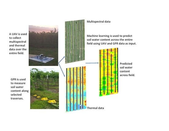
Assessing the Potential of UAV-Based Multispectral and Thermal Data to Estimate Soil Water Content Using Geophysical Methods

Abstract

Knowledge of the soil water content (SWC) is important for many aspects of agriculture and must be monitored to maximize crop yield, efficiently use limited supplies of irrigation water, and ensure optimal nutrient management with minimal environmental impact. Single-location sensors are often used to monitor SWC, but a limited number of point measurements is insufficient to measure SWC across most fields since SWC is typically very heterogeneous. To overcome this difficulty, several researchers have used data acquired from unmanned aerial vehicles (UAVs) to predict the SWC by using machine learning on a limited number of point measurements acquired across a field. While useful, these methods are limited by the relatively small number of SWC measurements that can be acquired with conventional measurement techniques. This study uses UAV-based data and thousands of SWC measurements acquired using geophysical methods at two different depths and before and after precipitation to predict the SWC using the random forest method across a vineyard in the central United States. Both multispectral data (five reflectance bands and eleven vegetation indices calculated from these bands) and thermal UAV-based data were acquired, and the importance of different reflectance data and vegetation indices in the prediction of SWC was analyzed. Results showed that when both thermal and multispectral data were used to estimate SWC, the thermal data contributed the most to prediction accuracy, although multispectral data were also important. Reflectance data contributed as much or more to prediction accuracy than most vegetation indices. SWC measurements that had a larger sample size and greater penetration depth (~30 cm sampling depth) were more accurately predicted than smaller and shallower SWC estimates (~18 cm sampling depth). The timing of SWC estimation was also important; higher accuracy predictions were achieved in wetter soils than in drier soils, and a light precipitation event also improved prediction accuracy.

1. Introduction

Soil moisture is a key parameter for agricultural water management and for research activities in fields ranging from climate prediction to flood risk assessment. In agriculture, knowledge of soil moisture is needed to determine the optimal timing and rate of irrigation to maximize crop production, as well as to optimize soil–fertilizer interactions. Optimal water management also helps to conserve limited water resources and increase the profitability of the crop, and it can be useful in avoiding soil salinization. Regulators can also use measurements of soil water content (SWC) to help validate pumping records, which can make water users more accountable and can contribute to a better balance between the water needs of agriculture and the environment.

Soil water content has conventionally been measured using sensors buried in the soil, such as time–domain reflectometry, tensiometers, and capacitance sensors [1,2,3,4]. Although these methods can provide accurate SWC measurements, they are point measurements and cannot capture the heterogeneity of SWC at the field scale. Satellite remote sensing techniques can also be used to estimate surface SWC [5,6]. Satellite-based techniques have the advantages of covering entire fields, high temporal resolution, accurate positioning, and low costs to individual users of the data. Sentinel-2 provides free data and has a spatial resolution of 10–20 m and a 5-day revisit frequency, and it is one of the satellites commonly used in agriculture today [7,8,9,10]. However, the acquisition and availability of satellite imagery depends on weather conditions, and the timing of the satellite imagery cannot be tailored to the specific needs of each researcher or farmer. Perhaps the largest disadvantage of satellite-based techniques is their coarse spatial resolution; even with the highest resolution data currently available, the pixels are too large to be useful for most precision agriculture applications [11,12,13,14,15,16]. Another significant disadvantage is the depth penetration of satellite data; for most satellites, the signal typically penetrates only the first few cm into the soil. This limitation is overcome by data from the NASA Soil Moisture Active Passive (SMAP) mission Level-4, which can penetrate down to 100 cm, but the coarse resolution (9 km) of these data [17,18] makes them less suitable for precision agriculture. Thus, satellite-based measurements are often insufficient for agricultural irrigation management [19,20,21].

Geophysical methods, such as ground penetrating radar (GPR) or electromagnetic methods, overcome some of the limitations of both point measurements and satellite data. Geophysical data can be collected with high resolution, and the sampling depth of most geophysical instruments is greater than that of satellite data, so the SWC in the root zone can be determined [22,23,24,25,26,27,28]. Geophysical data can also be acquired whenever the farmer or researcher desires, and it is not affected by cloud cover. Also, geophysical measurements do not disturb the soil, so they are more representative of truly in situ conditions than some types of point measurements. However, geophysical methods do have disadvantages, the most significant of which may be the cost of geophysical instruments and the expertise needed in processing some types of geophysical data, such as GPR measurements. Also, geophysical methods acquire data along selected traverses, so even though the resolution of individual measurements is much higher than for satellite data, the entire field is not covered. Finally, most geophysical instruments must be close to the ground to measure the SWC, and data cannot be collected over the top of more rigid vegetation, such as fully grown corn stalks. Thus, measurements must be collected parallel to crop rows for some types of vegetation, which may not be the desired traverse orientation.

In recent years, precision farming has begun to extensively utilize unmanned aerial vehicle (UAV) technology to provide information on crop health and make predictions about crop yield [29,30,31,32]. Unlike geophysical data, UAV-based data is acquired over the entire field. UAV instruments and sensors are less expensive than geophysical instruments, and data processing is usually simpler. Some advantages of UAV methods over satellite data are that UAV data are much higher resolution than satellite-based methods, they are collected below the level of most clouds, so are not obscured on cloudy days, and farmers can acquire data at the times they deem optimal, if weather conditions permit [11,12,13,14,15,16]. UAV data can also be acquired quickly over large areas, so they can be used for near real-time monitoring.

Although UAV-acquired data have several advantages over both geophysical and satellite-based methods, the main disadvantage of SWC monitoring is that UAV techniques cannot directly measure SWC. Instead, most UAV data are used to assess crop health. UAV techniques have been used to monitor crop status [33,34,35,36,37], map plant water stress and crop vitality [38,39,40,41,42,43], and predict yields in corn [44,45], rice [46,47], soybeans [31,48,49], and wheat [32,50,51,52], as well as other crops. Crop health is often characterized by vegetation indices, which are algebraic combinations of reflectance data (most often the red, green, blue, red-edge, and near-infrared bands) acquired from a multispectral sensor.

Although UAV-based sensors do not directly measure soil properties, some researchers have correlated point-based measurements of soil properties with UAV data. Several researchers have correlated SWC measurements acquired with time–domain reflectometry (TDR) with UAV imagery. Ref. [53] used multispectral and thermal UAV data to help estimate SWC. In this study, researchers installed TDR probes at 10 locations across a field at depths of 15 cm, 45 cm, and 76 cm. By taking measurements at different times, 125 SWC measurements were acquired, and three machine learning models (artificial neural networks, support vector machines, and genetic programming) were used to correlate the SWC to the multispectral and thermal data. Ref. [54] used TDR probes to measure the SWC in 25 plots planted with maize. In each plot, four TDR measurements were acquired at a depth of 10 cm, and four measurements were acquired at a depth of 20 cm, for a total of 200 TDR measurements. They also collected multispectral data (red, green, blue, NIR, thermal, and virtual red-edge bands) using a UAV, and they used four machine learning methods (partial least squares regression, K nearest neighbor, random forest regression, and backpropagation neural network) to correlate reflectance data to the SWC measurements. Ref. [55] arranged twenty soil moisture sensors in an experimental tea field and collected soil moisture data every hour during six UAV flights where they collected thermal images. The researchers then correlated the SWC and the thermal data using a Radial Basis Function Neural Network model and a Principal Component Analysis (PCA)-RBF model. In a slightly different application, Ref. [56] measured the electrical conductivity of saturated soil at 0–10, 10–20, and 20–30 cm soil depths before and after adding a saline solution in two experimental plots of quinoa. They then used multiple linear regression to evaluate whether UAV-acquired hyperspectral, thermal, and Lidar data could detect the effects of salt-treated water on plants.

Several other studies have correlated UAV-based data with gravimetric SWC measurements acquired by collecting soil samples. Ref. [57] used random forest and extreme learning methods to correlate 70 gravimetric SWC samples from a field of winter wheat at a depth of 0–10 cm to UAV hyperspectral data. In [58], 84 and 44 soil samples were acquired at two different times and were used to measure the gravimetric water content in a dryland field over a depth of 0–15 cm during two UAV flights. In this study, the texture temperature vegetation dryness index (TTVDI) was calculated using UAV-derived normalized vegetation index (NDVI), surface temperature from multispectral and thermal imagery, and soil texture. Their results show that the TTVDI has the potential to estimate the surface SWC from soil texture data and UAV imagery. In [59], UAV data were acquired over fields of alfalfa and oats, while 184 soil moisture samples and 14 soil texture measurements were collected. An artificial neural network model was used to predict the gravimetric SWC from the UAV-based data.

The research presented here differs from most studies relating to SWC and UAV-based data because geophysical methods are used to measure the SWC at thousands of locations within a field. The geophysical technique used is ground penetrating radar (GPR), which can acquire high-resolution data along traverses. Using GPR-derived estimates of SWC provides an extensive data set which allows for more effective use of machine learning algorithms, since sufficient data are available for both training and testing. This research is also novel because a larger number of variables are considered than is typical; correlations were developed using both multispectral and thermal data acquired using a UAV, SWC measurements were acquired at two depth intervals, and UAV data were acquired before and after precipitation. The research questions covered by this study are:

• How effectively can SWC be estimated using multispectral and thermal data acquired from a UAV when many SWC estimates are available for training?
• Which types of UAV-based data are most useful for estimating SWC?
• How does SWC sampling depth affect estimation from UAV-acquired data?
• Does the timing of data acquisition relative to precipitation affect the accuracy of SWC prediction?
• Are shallow SWC estimates more accurate when correlated with the UAV response from larger vegetation (grapevines) or shorter vegetation (mown grass)?

2. Materials and Methods

2.1. Study Area Description

The study site was a portion of a vineyard near St. James, Missouri, USA (Figure 1). The study area covers 2 hectares, has little topographic variation, and is planted with Concord and Cayuga grapes. The soil composition at the site is Glenstead, Rosati, and Harville silt loams with low sand content.

2.2. UAV Data Acquisition and Processing

2.2.1. Multispectral Data Acquisition and Processing

Multispectral (blue, green, red, red-edge, and NIR reflectance bands) and thermal data were acquired using a UAV over the research area on 19 June 2020 (Figure 2). Five ground control points (GCPs) were used for geo-referencing and position correction for both multispectral and thermal UAV data sets. The ground control points were set at each of the four corners and in the middle of the field (Figure 3a). Standard black and white ground control points were used for the multispectral data, while ground control points covered in aluminum foil were used for thermal data. To ensure the accurate creation of orthomosaic maps, the thermal ground control points were constructed with different shapes to uniquely identify each point.

UAV multispectral data acquisition was performed using a DJI Inspire 1 V2.0 UAV and Sentera Double 4K Lock & Go Sensor. The five bands of this sensor are blue, green, red, red-edge, and near-infrared. The flying height was 60 m with an image overlap ratio of 80%, achieving the ground sampling distance (GSD) of 1.72 cm/pixel.

UAV image processing was performed using the structure of the motion photogrammetric method in Agisoft Metashape software (version 1.8.4) developed by Agisoft LLC (St. Petersburg, Russia). In this method, images were aligned and geo-calibrated to create orthomosaic maps. For the multispectral data, the orthomosaic maps were used to output data for the five reflectance bands referenced above, and these data were then used to calculate eleven commonly used vegetation indices (VIs). The equations used to calculate each VI are given in

Table 1. Reflectance values from the multispectral and thermal sensors were used to calculate vegetation and thermal indices.

	Index	Equation	Reference
Multispectral	Chlorophyll Index Green (CIG)	CIG = (NIR/Green) − 1	[60]
	Chlorophyll Index Red-Edge (CIRE)	ClRE = (NIR/RedEdge) − 1	[61]
	Green Leaf Index (GLI)	GLI= (2Green − Red − Blue)/(2Green + Red + Blue)	[62]
	Green Normalized Difference Vegetation Index (GNDVI)	GNDVI = (NIR − Green)/(NIR + Green)	[63]
	Green–Red Vegetation Index (GRVI)	GRVI = NGRDI = (Green − Red)/(Green + Red)	[64]
	Modified Green–Red Vegetation Index (MGRVI)	MGRVI = (Green2 − Red2)/(Green2 + Red2)	[65]
	Modified Normalized Difference Water Index (NDWI)	NDWI = [(Blue + Green)/2 − (Infrared + Red)/2]/[(Blue + Green)/2 + (Infrared + Red)/2]	[66]
	Normalized Difference Red-Edge Index (NDRE)	NDRE = (NIR − RedEdge) /(NIR + RedEdge)	[67]
	Normalized Difference Vegetation Index (NDVI)	NDVI = (NIR − Red)/(NIR + Red)	[68]
	Red–Green–Blue Vegetation Index (RGBVI)	RGBVI = (Green2 − Blue × Red)/(Green2 + Blue × Red)	[65]
	Visible Atmospherically Resistant Index (VARI)	VARI = (Green − Red)/(Green + Red − Blue)	[69]
Thermal	Normalized Relative Canopy Temperature Index (NRCT)	NRCT = (Ti − Tmin)/(Tmax − Tmin) Ti represents the pixel temperature, Tmin and Tmax are the lowest and highest temperatures obtained from the thermal data, respectively.	[70]

. The one exception is the modified Normalized Difference Water Index (NDWI), which conventionally uses infrared data (from a thermal camera), and calculates the mean of the relevant bands, as shown in Table 1. For this project, the infrared reflectance was replaced with NIR in the NDWI calculation. This was undertaken to better evaluate SWC prediction using VI calculated only from data acquired with a multispectral camera; the impact of thermal data on SWC estimation accuracy was also considered but was determined separately from the VI calculated using standard multispectral data. Since the original equation of the NDWI requires data from both multispectral and thermal cameras, this index blurs the distinction between cameras. The modified NDWI equation used in this research uses data from only the multispectral camera.

2.2.2. Thermal Data Acquisition and Processing

Multispectral data were acquired first, then thermal data collection started but was interrupted approximately halfway through the flight by a light precipitation event (rain which totaled 0.2 mm of accumulation). Thermal data acquisition was paused for approximately one hour until all precipitation had ceased, then was resumed. Although no precipitation was forecast and was not desired on this day, this event provided a unique opportunity to compare the results before and after a light precipitation event, as will be discussed in Section 3.1. It was not possible to acquire a complete set of thermal data across the field both before and after precipitation, but this study compares the thermal data acquired in different portions of the field before and after precipitation. Fortunately, multispectral data could be acquired over the entire field before and after precipitation, so these data were collected. Multispectral and thermal data were collected in east–west trending traverses, starting from the southern end of the site, and concluding in the north (Figure 2).

Figure 2. (a) UAV data were collected in east–west trending traverses, starting in the southern end of the study area. The light green lines show the actual UAV path, while the red lines schematically show how the drone progressed across the field. (b) Thermal data were acquired in the southern portion of the field before precipitation (blue area) and in the northern portion of the field after precipitation (green area). (c) UAV thermal map for the study area (before and after rain).

Figure 2. (a) UAV data were collected in east–west trending traverses, starting in the southern end of the study area. The light green lines show the actual UAV path, while the red lines schematically show how the drone progressed across the field. (b) Thermal data were acquired in the southern portion of the field before precipitation (blue area) and in the northern portion of the field after precipitation (green area). (c) UAV thermal map for the study area (before and after rain).

Thermal imagery was acquired using a Zenmuse XT thermal camera. The spectral band of the thermal camera is long-wavelength infrared. The flying height of the thermal image is 60 m, and the image overlap of the front and side is 85%, which provided a GSD of 5.37 cm/pixel.

For the thermal imagery, the values in the thermal orthomosaic were converted to temperature values (degrees Celsius) using the Agisoft Raster Calculator. In addition to the temperature data, the Normalized Relative Canopy Temperature (NRCT) index was also calculated, as described in Table 1.

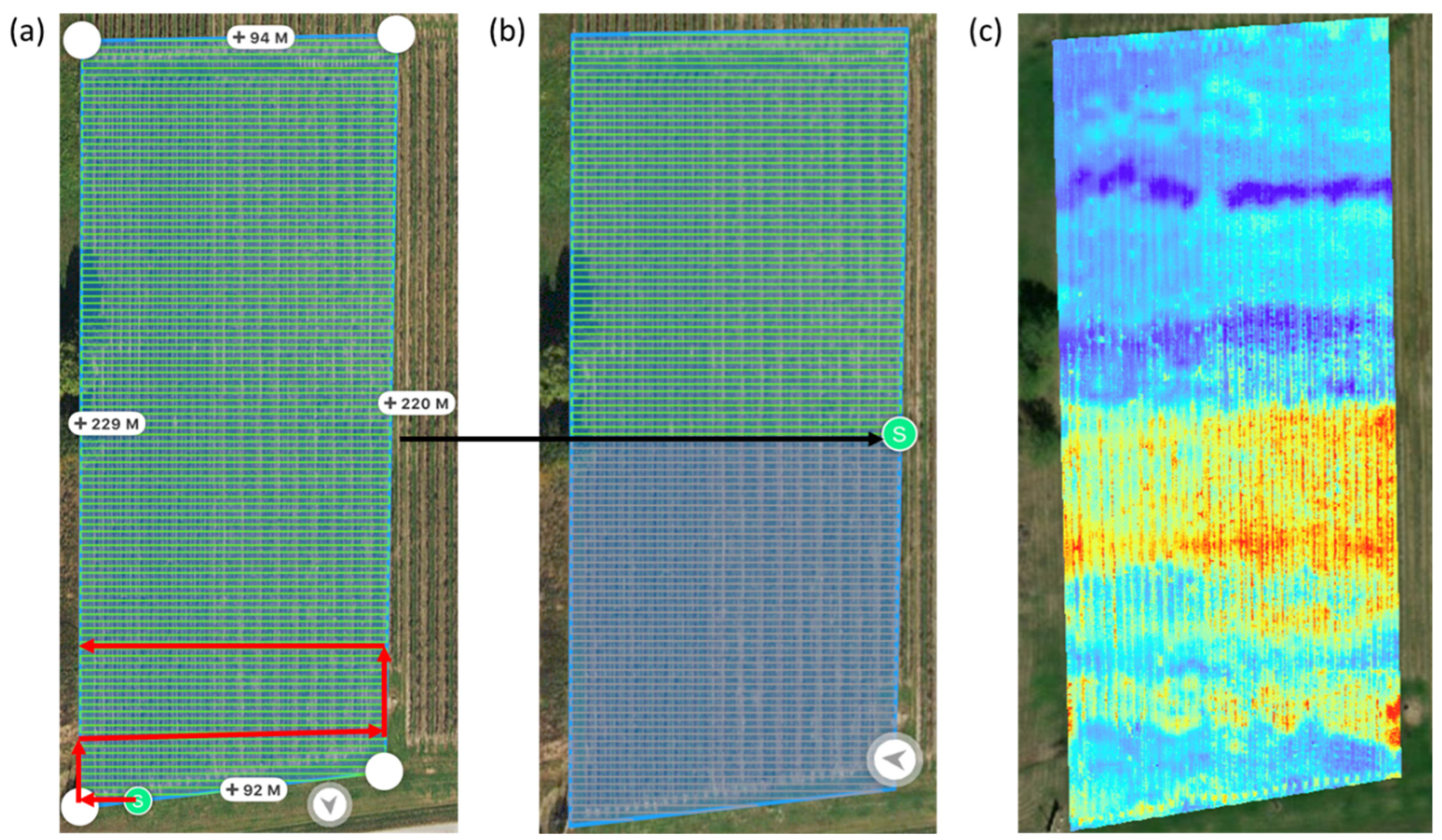
2.3. GPR Data Acquisition

GPR data were acquired using a bistatic PulseEkko system with 250 MHz and 500 MHz antennas. These frequencies were chosen because the sampling depth was greater than that of higher frequencies, while the antennas were easier to pull along the traverses than lower frequency antennas, which require the transmitting and receiving antennas to be moved separately. The GPR wavelet used to estimate the SWC was the groundwave, which is the energy that travels directly between the transmitting and receiving antennas. GPR groundwave energy has been successfully used to map SWC by many researchers [71,72,73,74,75,76,77,78,79,80] and is an established near-surface technique. To collect the groundwave data used in this study, five variable-offset surveys were first acquired in different locations around the field to establish an optimal antenna separation. The optimal antenna separation was established by choosing a separation where the groundwave was not superimposed with the airwave but still had sufficient amplitude to be easily identified during data analysis. Then, common-offset data were collected at this antenna separation at 10 cm intervals along the traverses shown in Figure 3a. Data were acquired continuously along the traverses, but some data had to be omitted due to interference between the groundwave and shallow reflections, so the traverses shown in Figure 3a show some areas of missing data. Similar to the thermal data, GPR data acquisition was paused during the light precipitation event. GPR data acquisition began on the eastern side of the field and progressed to the west, so the data acquired on the eastern portion of the field were obtained before precipitation. Data on the western side of the site were acquired after precipitation, as shown in Figure 3b. GPR data were acquired in the grassy area between grapevines but were closer to the grapevines than the center of the row (Figure 3c). Data were acquired at this location to avoid ruts due to machinery in the center of the row.

For each common-offset GPR measurement, the airwave and groundwave arrival times were identified, and the travel time of the groundwave was used to estimate the apparent dielectric permittivity (K_a) using the method described in [73]. The SWC was estimated from the apparent dielectric permittivity using Topp’s equation:

$$SWC=4.3\ast {10}^{-6}{K}_a^3-5.5\ast {10}^{-4}{K}_a^2+2.92\ast {10}^{-2}{K}_a-5.3\ast {10}^{-2}$$

(1)

which is an empirical model that was developed using a range of soils, is independent of soil texture, density, and temperature, and has an error estimate of 0.013 [81]. Due to its accuracy and ease of use, Topp’s equation is often used in studies of agricultural SWC.

Figure 3. (a) Multispectral map (before rain) with GPR traverses, which are shown as yellow lines. The red boxes mark the position of the ground control points. (b) GPR traverses acquired before the rain are shown as white lines, and the traverses acquired after the rain are shown as black lines. (c) GPR data (as shown by the yellow line) were collected in the grassy area between vines but were not in the center of the row.

Figure 3. (a) Multispectral map (before rain) with GPR traverses, which are shown as yellow lines. The red boxes mark the position of the ground control points. (b) GPR traverses acquired before the rain are shown as white lines, and the traverses acquired after the rain are shown as black lines. (c) GPR data (as shown by the yellow line) were collected in the grassy area between vines but were not in the center of the row.

The penetration depth of the GPR groundwave is a function of frequency [71], and the penetration depth of the 500 MHz and 250 MHz antennas are ~18 cm and ~30 cm, respectively [23]. Thus, the SWC measurements acquired with these two frequencies provide information about two depth intervals within the root zone.

2.4. Using Machine Learning to Correlate UAV-Based Data with SWC

Before the different data sets acquired in this research could be correlated, it was necessary to upscale the higher resolution UAV-based data to the same scale as the ground-based measurements. First, the multispectral and thermal data were upscaled to have the same pixel size of 15 cm by 12 cm, which allowed a better comparison of these data sets and reduced the computational requirements for further upscaling to the GPR footprint. For the 250 MHz GPR data, which has larger antennas and a greater antenna separation, the length of each measurement was 136 cm (the length of two antennas plus the distance between them) and the width was 38 cm (the width of the antenna). For the 500 MHz GPR data, the length and width were 84 cm and 23 cm, respectively. To correlate these data with the UAV-based measurements, each multispectral and thermal pixel whose centroid fell within the footprint of a GPR measurement was found. Upscaling was performed using SQL, where all multispectral and thermal data points whose pixel centroid location fell with a rectangle defined by the GPR centroid ±0.5 × GPR antenna width and ±0.5 × GPR antenna length were arithmetically averaged for comparison with that GPR measurement.

The machine learning method chosen to predict the SWC using UAV-based measurements was the random forest method. The random forest algorithm can efficiently handle large data sets and has provided more accurate predictions than some other machine learning algorithms [82,83,84]. Furthermore, random forest models are more stable with less training time than other methods, and they are typically easier to interpret [85]. The random forest method has been used in several studies that correlate remote sensing data with soil properties. In [54], random forest regression provided a more accurate prediction of SWC from UAV-based data than partial least squares regression, K nearest neighbor, and backpropagation neural networks. Ref. [86] found that the random forest algorithm performed better than the elastic net, general linear, or robust linear models for predicting SWC using UAV-acquired data. Ref. [87] used the random forest algorithm for predicting soil moisture in a peat bog. Ref. [88] used the random forest model with UAV-based data to predict SMC and soil electrical conductivity. Refs. [89,90] used random forest methods to estimate soil salinity using UAV hyperspectral imagery. Ref. [91] used a random forest algorithm with satellite data to predict soil pH, soil organic matter, and clay content. The random forest method was chosen for this study since this data set had a large number of measurements, preliminary analysis showed that non-linear correlations would likely be necessary, and understanding the relationships between input and output variables was desired. Other ML methods were not applied, so it should be noted that one of these other methods might yield better results for this experiment, but only one method was used here for the sake of brevity.

In this research, the random forest method was used to predict SWC, where multispectral reflectance data, vegetation indices, thermal data, and thermal indices were used as inputs to the model. First, all variables were normalized to a range from 0 to 1. Then, the data were randomly divided into five quintiles. Five quintiles were used to reduce the effects of outliers in any one quintile. For each quintile, 80% of the data were used for training, and the remaining 20% were used for testing. This division of data for training and testing was based on previous studies that suggested that this was the optimal division for allowing sufficient training to occur without overfitting the data [92]. The mean squared error (MSE), root mean square error (RMSE), and Pearson correlation coefficient (R²) were calculated for the 20% of data used for testing for each quintile. The arithmetic average of these values for all five quintiles was calculated and used as the representative value. The MSE is a common metric for calculating error; since it is a squared value, positive and negative values are weighted equally and do not cancel each other out. The RMSE is similar, but since it has the same units as the input variable, it is more intuitive to evaluate. The Pearson correlation coefficient was used since it is unitless and therefore provides an evaluation of correlation that is easy to understand without any reference to units.

To explore the efficacy of different data types, SWC prediction was first conducted using only multispectral data: blue, green, red, red-edge, and NIR, and the vegetation indices listed in Table 1. The thermal data were then added as inputs, and the random forest algorithm was repeated to see what additional benefit could be derived from the thermal data. Finally, machine learning was repeated a third time, this time using multispectral, VI, and the NRCT thermal index as inputs. The multispectral data were investigated first since these data are the least expensive and the most commonly acquired. The final analysis, using multispectral, VI, and NRCT data, was performed to determine if the thermal index would provide better predictions of the SWC than using simple temperature values.

As described in Section 2.2, the multispectral data were collected separately before and after the precipitation event. A comparison of the multispectral data acquired before and after precipitation showed little change in either the statistical or spatial distributions of reflectance values, which indicates that data repeatability was high. Although not intended, the precipitation event provided an opportunity to compare multispectral data sets, and the similarity of data acquired before and after precipitation served as a useful check of data quality. Thermal data were collected only once across the field, and the thermal data collection was interrupted by light precipitation. Although the precipitation was minimal, the temperature difference before and after precipitation was significant enough (Figure 2c) that the temperature data sets before and after precipitation had to be considered separately for prediction purposes. To perform machine learning, two sets of UAV-based files were therefore used. The multispectral data and thermal data acquired before precipitation were used for the southern half of the site, while the data sets acquired after precipitation were used for the northern half. Separate prediction results are provided for each half of the field.

While the UAV data were acquired starting on the southern side of the field and moving north, the GPR data were acquired starting from the eastern side of the field and working westward. Therefore, the portion of the field that had both GPR and UAV-based data acquired before precipitation was the southeast quadrant. The portion of the field that had all data acquired after precipitation was the northwest quadrant. To be consistent with all data sets, predictions were conducted separately for the southeast and northwest portions of the field. In addition to these quadrants, predictions were also completed for the entire southern half of the field (multispectral and thermal data acquired before precipitation, part of the GPR data acquired before precipitation, and partly acquired after precipitation) and for the entire northern half of the field (multispectral and thermal data acquired after precipitation, part of the GPR data acquired before precipitation, and partly acquired after precipitation). The different portions of the field that were analyzed separately are shown in Figure 4. Although the authors recognize that less accurate predictions should be expected when some of the SWC data were acquired before precipitation and some were acquired afterward, these predictions were attempted because the change in the average SWC (as estimated by the difference in the average SWC in the northwest and southeast portions of the field) was fairly small (ΔSWC = 0.024) compared to the variability of the SWC across the field. Additionally, comparing predictions for the southeast quadrant with predictions made from the entire southern half of the field, or comparing predictions from the northwest quadrant with predictions from the entire northern half of the field, provides information on how this method may work when the SWC measurements are less accurate, as is often the case with other types of SWC measurements.

In addition to considering SWC prediction based on the timing of precipitation, the relationship between taller and shorter vegetation and SWC prediction was also investigated. To do this, random forest regression was first conducted using reflectance data and SWC values that were acquired at the same locations. These models represent the short vegetation. Next, the reflectance data acquired over the grapevines directly adjacent to the SWC measurements were used for SWC prediction. These models represent taller vegetation, and the SWC measurements were acquired under or near the edge of the grapevine canopy.

3. Results

3.1. Soil Water Content

The SWC across the vineyard varied for both the 500 MHz and 250 MHz data.

Table 2. Summary statistics for SWC estimates.

SWC from 500 MHz GPR (Sampling Depth ~ 18 cm)
Southeast Quadrant			Southern Half			Northwest Quadrant			Northern Half
Mean	SD	Count	Mean	SD	Count	Mean	SD	Count	Mean	SD	Count
0.174	0.053	6217	0.191	0.052	10,541	0.218	0.040	2491	0.180	0.049	7283
SWC from 250 MHz GPR (Sampling Depth ~ 30 cm)
Southeast Quadrant			Southern Half			Northwest Quadrant			Northern Half
Mean	SD	Count	Mean	SD	Count	Mean	SD	Count	Mean	SD	Count
0.164	0.042	6265	0.168	0.044	10,724	0.188	0.042	2571	0.159	0.046	6590

shows the summary statistics for SWC estimates obtained from both GPR frequencies for data acquired before and after precipitation. As expected, the SWC was slightly lower before precipitation (SE quadrant) and slightly higher after precipitation (NW quadrant) for both sampling depths, while the data sets that were collected partially before and partially after precipitation (southern and northern halves) showed intermediate SWC. The shallower soil (measured by the 500 MHz data) was slightly wetter than the deeper soil for all data sets. A greater SWC difference was observed in the shallower 500 MHz data before and after precipitation, which indicates that the small amount of precipitation received did not penetrate very far into the subsurface or influence a deeper soil volume. SWC variability was somewhat higher for the shallower measurements in the drier soil, while the deeper/larger volume measurements showed approximately the same variability for all data sets. Figure 5a and Figure 6a show the SWC distribution across the study area for both frequencies.

3.2. SWC Prediction Using Random Forest Method

Table 3. SWC prediction at two sampling depths.

	Prediction of SWC from 500 MHz GPR (Sampling Depth ≈ 0.18 m)
	Southeast Quadrant		Southern Half		Northwest Quadrant		Northern Half
	R2	RMSE	R2	RMSE	R2	RMSE	R2	RMSE
Multispectral	0.404	0.135	0.424	0.145	0.555	0.146	0.449	0.134
Multispectral + Thermal	0.557	0.117	0.555	0.128	0.727	0.114	0.574	0.118
Multispectral + Thermal index NRCT	0.548	0.118	0.565	0.127	0.727	0.114	0.584	0.116
	Prediction of SWC from 250 MHz GPR (Sampling Depth ≈ 0.30 m)
	Southeast Quadrant		Southern Half		Northwest Quadrant		Northern Half
	R2	RMSE	R2	RMSE	R2	RMSE	R2	RMSE
Multispectral	0.628	0.100	0.582	0.109	0.799	0.084	0.759	0.078
Multispectral + Thermal	0.743	0.084	0.704	0.092	0.879	0.066	0.830	0.066
Multispectral + Thermal index NRCT	0.735	0.084	0.696	0.093	0.882	0.065	0.831	0.066

shows the correlation coefficient (R²) and RMSE for predictions of SWC for the 20% of data used for testing using different input parameters, sampling depths, and timing of precipitation. The prediction results for each of these scenarios are discussed below and are shown in Figure 5 and Figure 6 for the 500 MHz and 250 MHz results, respectively. The same SWC prediction scale is used for all sub-figures, although the scales between Figure 5 and Figure 6 are slightly different.

3.2.1. Input Parameters

As described in Section 2.4, the random forest models were conducted using different input parameters: only multispectral data, multispectral with thermal data, and multispectral with NRCT data. Multispectral data included reflectance data as well as the vegetation indices described in Table 1. Table 3 shows that for both GPR frequencies (corresponding to two different SWC sampling depths) and for all soil moisture conditions (before precipitation, after precipitation, or mixed), using only multispectral data provides a reasonable degree of prediction accuracy, but the accuracy increases substantially when thermal data are also included.

To further evaluate which types of multispectral or thermal data were most useful for SWC prediction, the random models were run multiple times for each set of input parameters (only multispectral data, multispectral and thermal data, and multispectral and NRCT). To establish a benchmark for accuracy, estimation was first performed using all the parameters in a given category (i.e., all the multispectral data). Then, random forest prediction was repeated, but one of the input parameters was omitted from the model. This was repeated until predictions had been run for all parameters, omitting one parameter each time. The parameters that resulted in the greatest increase in prediction error due to their omission were considered the most important.

Table 4. The relative importance of different types of UAV-based data for SWC prediction from 500 MHz data.

The Most Important UAV-Based Data for Predicting SWC, 500 MHz GPR
Ranking	Southeast Quadrant			Northwest Quadrant
	Multispectral	Multispectral + Thermal	Multispectral + NRCT	Multispectral	Multispectral + Thermal	Multispectral + NRCT
1	NIR band	Thermal temperature	NRCT	NIR band	Thermal temperature	NRCT
2	NDVI	Green band	Red-edge band	MGRVI	VARI	VARI
3	Red band	Blue band	Green band	Green band	Green band	NDVI
Ranking	Southern Half			Northern Half
	Multispectral	Multispectral + Thermal	Multispectral + NRCT	Multispectral	Multispectral + Thermal	Multispectral + NRCT
1	Red band	Thermal temperature	NRCT	Red band	Thermal temperature	NRCT
2	CIG	Red band	NDWI	CIG	Blue band	Blue band
3	NIR band	CIG	NDVI	NIR band	VARI	NDWI

shows which parameters were most important for predicting the SWC for the southeast quadrant (all data acquired before precipitation), the northwest quadrant (all data acquired after precipitation), and the northern and southern halves (mixed data acquisition) for the 500 MHz SWC data.

Table 5. The relative importance of different types of UAV-based data for SWC prediction from 250 MHz data.

The Most Important UAV-Based Data for Predicting SWC, 250 MHz GPR
Ranking	Southeast Quadrant			Northwest Quadrant
	Multispectral	Multispectral + Thermal	Multispectral + NRCT	Multispectral	Multispectral + Thermal	Multispectral + NRCT
1	GLI	Thermal temperature	NRCT	MGRVI	Thermal temperature	NRCT
2	CIG	CIG	Blue band	Red band	NDRE	Green band
3	Green band	VARI	CIG	Green band	Red band	NDVI
Ranking	Southern Half			Northern Half
	Multispectral	Multispectral + Thermal	Multispectral + NRCT	Multispectral	Multispectral + Thermal	Multispectral + NRCT
1	Red-edge band	Thermal temperature	NRCT	CIG	Thermal temperature	NRCT
2	NIR band	CIG	Red band	RGBVI	NDWI	Blue band
3	CIG	Green band	Green band	Blue band	Green band	NDVI

repeats this analysis for the 250 MHz SWC data.

Table 4 shows that for the shallower SWC measurements (500 MHz data), a few reflectance bands or VI are consistently important. When only multispectral measurements are used, the NIR reflectance is important for both individual quadrants of the field (before and after precipitation) and for the two halves of the field (mixed before and after precipitation). The red reflectance band is also important for most of these areas. Overall, the NIR, red, and green bands are the most important for the multispectral data, as all the most influential parameters were either these bands individually or a combination of these bands (NDVI, MGRVI, CIG). When either temperature data (thermal) or NRCT data were added to the prediction parameters, the temperature-based measurements were the most influential for SWC prediction. Including the thermal data changed which multispectral bands were most influential; when the thermal data were included, the blue reflectance band became important, both as a direct reflectance band and because it is an input to VI such as VARI, MGRVI, and NDWI, which use a combination of blue, green, red, and NIR bands.

Table 5 shows that the deeper SWC measurements (250 MHz data) differ somewhat in which parameters are most influential. When only multispectral data are considered, different parameters are important for different portions of the field; the only parameter that is important for most portions of the field is CIG, which uses the NIR and green bands. Similar to the 500 MHz data, when temperature or NRCT data are added, these data are the most influential parameters for predicting SWC. Other important parameters vary depending on the portion of the field considered, but CIG and green, red, and blue reflectance bands are typically the most important.

3.2.2. Sampling Depth

Comparing prediction results for SWC estimates obtained from the 500 MHz and 250 MHz GPR data can provide insights into how the depth of the SWC measurement affects correlations with the multispectral and thermal data. Table 3 shows that for all soil moisture conditions, the SWC calculated with the 250 MHz data (sampling depth of ~30 cm) is more easily predicted using multispectral and thermal data than the SWC calculated with the shallower (~18 cm) penetration depth of 500 MHz antennas. Possible explanations for the better performance of the 250 MHz data are discussed in Section 4.2. The lower correlation coefficients and higher RMSE of the 500 MHz data indicate that this higher frequency may not produce estimates that are accurate enough for many applications.

3.2.3. Soil Moisture/Precipitation

Table 3 shows that for both GPR frequencies, the best predictions of SWC occurred when both the SWC and multispectral/thermal data were acquired after precipitation (northwest quadrant). Intermediate levels of correlation were observed when the SWC data were acquired partially before and partially after precipitation (northern and southern halves, considered separately), and the least correlation occurred when both the SWC and multispectral/thermal data were acquired before precipitation (southeast quadrant). As discussed in Section 4.3, this may be due to changes in the reflectance of the vegetation after precipitation.

3.3. Impact of Short vs. Tall Vegetation on SWC Prediction

The SWC in the root zone is affected by both more shallowly rooted vegetation (such as grass) and by larger vegetation (such as grapevines) which have both shallow and deep roots [93,94]. Some researchers who studied whether multispectral data acquired in orchards could be used to predict SWC used the response of the tree canopy and filtered out the response from grass or bare soil [41]. In this study, SWC measurements were acquired slightly to one side of the grapevines instead of near the grapevine trunks (Figure 3c). SWC measurements were collected at this location to allow the GPR antennas to be pulled continuously down the rows while maintaining full contact with the ground, which is necessary for high-quality data. The ground cover where the SWC measurements were acquired was short (mown) grass. To determine whether the SWC was more highly correlated to the grapevines, whose roots extended into the areas where the SWC was measured, or to the short grass, machine learning predictions were also performed by correlating the SWC measurements with the multispectral and thermal data collected directly adjacent to the SWC measurements but fully over the grapevines. The sample footprint remained the same for upscaling, but the location of each multispectral and thermal measurement used in the prediction was slightly to the west of the actual SWC measurement location so that the UAV-based measurements aligned fully with the grapevine canopy.

Table 6. SWC prediction metrics when UAV-based data are collected over the grapevines.

Prediction of SWC from 500 MHz GPR Using Grapevine Canopy Data
Data Set	Southeast Quadrant		Southern Half		Northwest Quadrant		Northern Half
	R2	RMSE	R2	RMSE	R2	RMSE	R2	RMSE
Multispectral	0.262	0.151	0.284	0.162	0.45	0.162	0.479	0.131
Multispectral + Thermal	0.427	0.133	0.457	0.141	0.564	0.145	0.578	0.118
Multispectral + NRCT	0.432	0.133	0.435	0.144	0.565	0.144	0.575	0.118
Prediction of SWC from 250 MHz GPR Using Grapevine Canopy Data
Data Set	Southeast Quadrant		Southern Half		Northwest Quadrant		Northern Half
	R2	RMSE	R2	RMSE	R2	RMSE	R2	RMSE
Multispectral	0.514	0.115	0.423	0.128	0.66	0.110	0.664	0.092
Multispectral + Thermal	0.68	0.093	0.579	0.109	0.785	0.087	0.776	0.076
Multispectral + NRCT	0.688	0.092	0.571	0.110	0.778	0.089	0.772	0.076

shows the results of these predictions. A comparison of Table 3 and Table 6 shows that for all sampling depths and SWC (wet or dry) combinations, the SWC could be predicted more accurately when the UAV-based measurements were acquired over the shorter vegetation (and directly over the SWC measurements) than when these measurements were acquired over the larger vegetation closest to the SWC measurements.

4. Discussion

4.1. Input Parameters

Table 3, Table 4 and Table 5 show that multispectral data can be used for SWC prediction, but that the prediction accuracy increases significantly when thermal data are added to the ML algorithm. In this study, temperature data and NRCT provided approximately the same amount of increased prediction accuracy (Table 3), indicating that normalizing the temperature data made little difference in prediction accuracy. Table 4 and Table 5 show that temperature or NRCT were the most important single parameters for estimating SWC when multiple data types were investigated.

Table 4 shows that when only multispectral data are used to estimate SWC, the NIR, red, and green reflectance bands were the most important parameters for most of the field for the shallower soil (500 MHz). CIG (calculated using NIR and green reflectance) was also an important parameter. Since healthy vegetation usually strongly reflects green and NIR wavelengths, and soil has a stronger red reflectance, the strong correlation between SWC and these parameters is probably indicative of the correlation between vegetation vigor (strong direct correlation with green and NIR reflectance and strong inverse correlation with red reflectance) and SWC. For the deeper SWC measurements (250 MHz), similar reflectance bands or VI are still important (especially CIG), but the blue reflectance band is more significant since it occurs both as an individual reflectance band and within VI such as GLI and RGBVI. The increased importance of the blue band for predicting SWC from the 250 MHz GPR data may be related to the ability of the blue reflectance band to distinguish soil from vegetation [95]. For the 250 MHz data, the sample footprint is wider than for the 500 MHz data, and the 250 MHz footprint sometimes included areas of bare soil nearer to the grapevine trunks (Figure 3c). Since the SWC in bare soil is usually different than the SWC where cover crops exist [73], the blue reflectance band may be beneficial in distinguishing this difference.

When thermal data are included in the SWC estimation, the VARI (calculated from green, blue, and red reflectance bands) and the green and blue bands were the most important parameters after the thermal input for both the shallower and deeper SWC estimates. This indicates that including thermal data reduces the significance of the NIR reflectance for SWC estimation; these bands may respond to similar vegetative or soil properties. However, both NDWI and NDVI are important parameters, especially for the deeper 250 MHz measurements. Since these parameters both use NIR as input (as calculated for this study), this implies that NIR still offers useful correlations with SWC and should not be omitted even when thermal data are also collected.

4.2. Sampling Depth

Table 3 indicates that a more accurate prediction of the SWC was possible with samples that had a greater sampling depth (SWC from 250 MHz GPR, sampling interval from 0 to ~30 cm) as compared to shallower samples (SWC from 500 MHz GPR, sampling interval from 0 to ~18 cm). The higher correlation of multispectral and thermal data with the deeper SWC data may occur because more of the vegetation root structure occurs somewhat deeper in the surface. For grapevines, most small roots are at a depth of 10 to 60 cm, while larger roots occur at depths of 18 to 80 cm [93]. Approximately 30–40% of the grapevine roots occur in the interval from the surface to 30 cm depth [96], and grapevine roots extend from the vine outward to more than a meter over this depth interval [97], which includes the zone sampled by the GPR. In addition to vine roots, the roots of most grasses that grow between the rows extend to a depth of more than 50 cm, although the highest grass root density is within the uppermost 10 cm [98]. The sampling depth of the 500 MHz data would therefore encompass primarily small grapevine roots and grass, while the 250 MHz sampling depth encompasses both small and large grapevine roots and grass roots. Since the vegetation vigor measured by the reflectance data is partially determined by the plant root structure, samples that encompass a greater percentage of the root structure are more likely to correlate to vegetation vigor. Thus, the SWC estimates acquired with the 250 MHz antenna are expected to better correlate with multispectral data.

Another possible reason that the 250 MHz data better correlates with multispectral data is that the sampling volume of the 250 MHz data is greater than that of the 500 MHz data. Both the footprint and the sampling depth of the 250 MHz antennas are larger than that of the 500 MHz antennas; the approximate volume measured by the 250 MHz antennas is 0.04 m³, while that of the 500 MHz antennas is 0.01 m³. The larger sampling volume of the 250 MHz antennas means that some small-scale SWC variability is lost within the sampling volume, whereas the smaller 500 MHz data show more variability. Table 2 supports this assumption since the standard deviation of the SWC is usually less for the 250 MHz than for the 500 MHz data. Prediction is generally easier when variability is less, so the higher correlation of the 250 MHz data may be the result of sample volume.

4.3. Average SWC/Precipitation

The unique timing of data acquisition for this project (before and immediately after a light precipitation event) permits the evaluation of the effects of average SWC and precipitation on SWC prediction. Since UAVs are usually flown only in clear, sunny conditions [31,34,35,37,38,40,41,46,49,50,51,52], the effect of precipitation is not usually considered. The data from this study indicates that both average SWC and recent precipitation change the SWC prediction accuracy.

To evaluate the effects of average SWC, wet or dry quadrants of the field can be compared to the half-sections of the field. For example, a more accurate prediction of SWC occurred over the southern half of the field than over the SE quadrant, although all UAV-based data for the southern half of the field were acquired before precipitation. The SE quadrant of the field was drier than the southern half of the field, which shows that the SW quadrant was wetter than the SE quadrant. Higher SWC prediction accuracy in the southern half, as compared to the SE quadrant, shows that wetter soils allowed better prediction of the SWC than drier soil. Similarly, the NW quadrant was wetter than the northern half of the field, and prediction of the SWC was better in this quadrant than in the northern half, although all UAV-based data for the northern half of the field were acquired after precipitation. One reason that prediction accuracy might be better in wetter soils is that wetter soils could allow more accurate sensing of root density. When more water is available in the soil, more water can be absorbed by the roots. Since the GPR measurements do not distinguish between water held in soil pores versus water held by plant roots, the measured SWC could be a proxy for root density if there are many roots in the measured volume. Since vegetation vigor is strongly influenced by roots, correlations between multispectral data and SWC are expected to be higher when root density is greater. Another possible explanation for the increased SWC prediction accuracy in wetter soils is that increased SWC caused differences in soil texture to be accentuated. In the vadose zone, finer-grained soils will absorb and retain moisture, while coarser-grained soils more easily allow water to be transmitted through them. The small amount of precipitation received during this study might have served to better distinguish differences in soil texture, and long-term vegetation vigor may be influenced by the soil texture.

The effects of precipitation on multispectral data are not often analyzed, but this study suggests that precipitation may also affect the prediction of SWC based on multispectral data. This conclusion can be drawn by considering data from both halves of the field. Both halves have SWC values that were partially collected before the light precipitation event and partially collected afterward, but the SWC for the northern half of the field was predicted using multispectral and thermal data acquired after precipitation, while the SWC for the southern half of the field was predicted using multispectral and thermal data acquired before precipitation. The average SWC values in both halves of the field are very similar (differing by only 0.01), as shown in Table 2. However, SWC predictions were better in the northern half of the field (Table 3), suggesting that the light precipitation event influenced prediction.

The light precipitation event may have influenced SWC prediction by washing away the dust that may have accumulated on the leaves or grass. Healthy vegetation usually has strong reflectance in green, red-edge, and NIR wavelengths. Chlorophyll strongly reflects green wavelengths but reduces the reflection from blue wavelengths. Water usually has higher reflectance in the blue and green wavelengths but absorbs red-edge and NIR wavelengths [99,100]. If the precipitation removed dust from the leaves/grass, the chlorophyll could be more easily detected, and a strong reflectance would be expected in the green wavelength, while a lower reflectance would occur in the blue wavelength. However, if water remained on the leaves, the blue reflectance might increase from that source.

Table 7. Mean reflectance over the entire field before and after precipitation.

	Blue	Green	Red	Red-Edge	NIR
Before precipitation	43.42	96.414	65.093	140.19	63.766
After precipitation	40.194	97.197	63.984	138.879	59.88

shows the mean value of multispectral reflectance data for the entire field before and after precipitation. This table shows a slight increase in green reflectance and a more significant decrease in blue reflectance, as well as a decrease in NIR. These results indicate that for this site, the effects of chlorophyll could be more easily observed after precipitation, but residual water on the leaves may have reduced other wavelengths, like NIR.

4.4. Impact of Short vs. Tall Vegetation on SWC Prediction

A comparison of Table 3 and Table 6 shows that predictions of SWC were generally more accurate when multispectral and thermal data were acquired directly over the SWC measurement point than when these measurements were acquired over the grapevines immediately adjacent to the measurements. This suggests that although the grapevine vigor is clearly related to nearby SWC (Table 6), the effects of cover crops (such as grass at this site) are also significant. This result matches that found by other researchers [73,97,101,102], where cover crops were found to have a significant impact on the SWC in vineyards. It is probable that a better correlation between multispectral data acquired over the vines and SWC might have resulted if SWC was measured over a deeper interval than was performed in this study, since grapevines have been shown to develop deeper root systems than the cover crops (grass in this study) in vineyards where cover crops are regularly used [101].

4.5. Other Factors

While outside the scope of this experiment, it is important to note that other factors can also impact soil water content, and thus may change the accuracy of SWC prediction using these methods. One factor to consider is crop type. This experiment was conducted on a vineyard with a cover crop, and while previous research showed that this technique could be effective in row crops such as maize and soybeans [88], it is not clear if this technique will work on non-row crops or non-agricultural vegetation. Allowing weeds to grow between the rows of a cash crop might also have a different impact on SWC than cover crops. Another consideration is farming practices; frequent tilling or compaction due to agricultural equipment might change the soil structure and could reduce the efficacy of this technique. Irrigation practices must also be considered, as drip irrigation could result in SWC heterogeneity that may decrease the correlation between UAV-based reflectance measurements and actual soil conditions.

Another factor that should be considered is the accuracy of the SWC measurements obtained with geophysical methods. While GPR groundwaves are non-invasive and therefore do not introduce inaccuracy resulting from soil disturbance during probe insertion, the estimates of SWC are made using geophysical parameters rather than a direct measurement of soil water. A petrophysical relationship must therefore be used to convert from geophysical parameters to SWC. While the petrophysical relationship used in this study to convert dielectric permittivity to SWC is very commonly applied to agricultural soils, a site-specific petrophysical relationship would be more accurate; higher accuracy SWC estimates might improve the correlation with UAV data. Another consideration for applying this technique is that UAV flight parameters must be chosen carefully to provide sufficiently detailed orthomosaic images. If insufficient ground control points are used, or if the UAV is flown too high or too quickly, the data may be insufficient to construct an accurate orthomosaic, which will also affect the final estimation accuracy.

5. Conclusions

This study showed that UAV-mounted sensors can be used for SWC prediction using machine learning techniques when a sufficiently large number of SWC measurements are available. Of the data types tested in this study, thermal data were the most important for predicting SWC, although multispectral data were also necessary for accurate predictions. Reflectance data (red, green, blue, and NIR) correlated with SWC measurements as well as or better than most VI, indicating that these bands ought to be included in machine learning techniques. Predictions of SWC were more accurate for deeper and larger volume SWC measurements than for shallower, smaller measurements. The value of the SWC measurement as well as the timing of the UAV flight also influenced prediction accuracy; accuracy was better in wetter soils and after precipitation. Finally, accuracy was highest when considering the multispectral data acquired directly over the SWC measurement instead of using the larger vegetation canopy directly adjacent to the SWC measurement. It should also be noted that although the correlation coefficients between estimated and actual SWC were quite high for the data acquired under optimal conditions (wetter soil and deeper measurements), collecting data under different conditions may result in lower correlations. Also, the RMSE was still relatively high, so this method may be better for indicating the spatial distribution of SWC and for selecting the locations for conventional measurements if very accurate SWC values are needed.

The methodology used in this study has potential to provide SWC estimates with much higher resolution than is currently available from remote sensing data. Higher resolution SWC estimates could be used to better guide precision agriculture by directing the timing and volume of infiltration as well as the timing of nutrient application. This technique could also be applied to environmental and climate change studies, since SWC is a critical parameter in climate modeling and heat flux calculations. Finally, UAV-based estimates of SWC could also be helpful for predicting natural hazards, such as floods and landslides. For floods, the SWC is important because it strongly influences the partitioning of precipitation into infiltration or surface runoff. SWC affects landslides because soil strength and weight are greatly affected by SWC, and these factors affect slope stability.

References

1. Bittelli, M. Measuring Soil Water Content: A Review. HortTechnology 2011, 21, 293–300. [Google Scholar] [CrossRef]
2. Robinson, D.A. Field Estimation of Soil Water Content: A Practical Guide to Methods, Instrumentation and Sensor Technology. Soil Sci. Soc. Am. J. 2009, 73, 1437. [Google Scholar] [CrossRef]
3. Robinson, D.A.; Campbell, C.S.; Hopmans, J.W.; Hornbuckle, B.K.; Jones, S.B.; Knight, R.; Ogden, F.; Selker, J.; Wendroth, O. Soil Moisture Measurement for Ecological and Hydrological Watershed-Scale Observatories: A Review. Vadose Zone J. 2008, 7, 358–389. [Google Scholar] [CrossRef]
4. Walker, J.P.; Willgoose, G.R.; Kalma, J.D. In Situ Measurement of Soil Moisture: A Comparison of Techniques. J. Hydrol. 2004, 293, 85–99. [Google Scholar] [CrossRef]
5. Palanisamy, S.; Selvaraj, R.; Ramesh, T.; Ponnusamy, J. Applications of Remote Sensing in Agriculture—A Review. Int. J. Curr. Microbiol. Appl. Sci. 2019, 8, 2270–2283. [Google Scholar] [CrossRef]
6. Peng, J.; Loew, A.; Merlin, O.; Verhoest, N.E.C. A Review of Spatial Downscaling of Satellite Remotely Sensed Soil Moisture. Rev. Geophys. 2017, 55, 341–366. [Google Scholar] [CrossRef]
7. Jiang, Y.; Lu, Z.; Li, S.; Lei, Y.; Chu, Q.; Yin, X.; Chen, F. Large-Scale and High-Resolution Crop Mapping in China Using Sentinel-2 Satellite Imagery. Agriculture 2020, 10, 433. [Google Scholar] [CrossRef]
8. Karlson, M.; Bayala, J.; Ouedraogo, A.; Soro, B.; Knorring, H.; Reese, H.; Ostwald, M. The Potential of Sentinel-2 for Crop Production Estimation in a Smallholder Agroforestry Landscape, Burkina Faso. Front. Environ. Sci. 2020, 8, 85. [Google Scholar] [CrossRef]
9. López-Andreu, F.J.; Erena, M.; Dominguez-Gómez, J.A.; López-Morales, J.A. Sentinel-2 Images and Machine Learning as Tool for Monitoring of the Common Agricultural Policy: Calasparra Rice as a Case Study. Agronomy 2021, 11, 621. [Google Scholar] [CrossRef]
10. Segarra, J.; Buchaillot, M.L.; Araus, J.L.; Kefauver, S.C. Remote Sensing for Precision Agriculture: Sentinel-2 Improved Features and Applications. Agronomy 2020, 10, 641. [Google Scholar] [CrossRef]
11. Berni, J.A.J.; Zarco-Tejada, P.J.; Suarez, L.; Fereres, E. Thermal and Narrowband Multispectral Remote Sensing for Vegetation Monitoring From an Unmanned Aerial Vehicle. IEEE Trans. Geosci. Remote Sens. 2009, 47, 722–738. [Google Scholar] [CrossRef]
12. Bian, Z.; Roujean, J.-L.; Cao, B.; Du, Y.; Li, H.; Gamet, P.; Fang, J.; Xiao, Q.; Liu, Q. Modeling the Directional Anisotropy of Fine-Scale TIR Emissions over Tree and Crop Canopies Based on UAV Measurements. Remote Sens. Environ. 2021, 252, 112150. [Google Scholar] [CrossRef]
13. Ma, Y.; Chen, H.; Zhao, G.; Wang, Z.; Wang, D. Spectral Index Fusion for Salinized Soil Salinity Inversion Using Sentinel-2A and UAV Images in a Coastal Area. IEEE Access 2020, 8, 159595–159608. [Google Scholar] [CrossRef]
14. dos Santos, L.M.; de Souza Barbosa, B.D.; Diotto, A.V.; Andrade, M.T.; Conti, L.; Rossi, G. Determining the Leaf Area Index and Percentage of Area Covered by Coffee Crops Using UAV RGB Images. IEEE J. Sel. Top. Appl. Earth Obs. Remote Sens. 2020, 13, 6401–6409. [Google Scholar] [CrossRef]
15. Sankey, J.B.; Sankey, T.T.; Li, J.; Ravi, S.; Wang, G.; Caster, J.; Kasprak, A. Quantifying Plant-Soil-Nutrient Dynamics in Rangelands: Fusion of UAV Hyperspectral-LiDAR, UAV Multispectral-Photogrammetry, and Ground-Based LiDAR-Digital Photography in a Shrub-Encroached Desert Grassland. Remote Sens. Environ. 2021, 253, 112223. [Google Scholar] [CrossRef]
16. Zarco-Tejada, P.J.; González-Dugo, V.; Berni, J.A.J. Fluorescence, Temperature and Narrow-Band Indices Acquired from a UAV Platform for Water Stress Detection Using a Micro-Hyperspectral Imager and a Thermal Camera. Remote Sens. Environ. 2012, 117, 322–337. [Google Scholar] [CrossRef]
17. Reichle, R.H.; Liu, Q.; Koster, R.D.; Crow, W.T.; De Lannoy, G.J.M.; Kimball, J.S.; Ardizzone, J.V.; Bosch, D.; Colliander, A.; Cosh, M.; et al. Version 4 of the SMAP Level-4 Soil Moisture Algorithm and Data Product. J. Adv. Model. Earth Syst. 2019, 11, 3106–3130. [Google Scholar] [CrossRef]
18. Zhao, B.; Dai, Q.; Zhuo, L.; Zhu, S.; Shen, Q.; Han, D. Assessing the Potential of Different Satellite Soil Moisture Products in Landslide Hazard Assessment. Remote Sens. Environ. 2021, 264, 112583. [Google Scholar] [CrossRef]
19. Crow, W.T.; Berg, A.A.; Cosh, M.H.; Loew, A.; Mohanty, B.P.; Panciera, R.; de Rosnay, P.; Ryu, D.; Walker, J.P. Upscaling Sparse Ground-Based Soil Moisture Observations for the Validation of Coarse-Resolution Satellite Soil Moisture Products. Rev. Geophys. 2012, 50. [Google Scholar] [CrossRef]
20. Inoue, Y. Satellite- and Drone-Based Remote Sensing of Crops and Soils for Smart Farming—A Review. Soil Sci. Plant Nutr. 2020, 66, 798–810. [Google Scholar] [CrossRef]
21. Martínez-Fernández, J.; González-Zamora, A.; Sánchez, N.; Gumuzzio, A.; Herrero-Jiménez, C.M. Satellite Soil Moisture for Agricultural Drought Monitoring: Assessment of the SMOS Derived Soil Water Deficit Index. Remote Sens. Environ. 2016, 177, 277–286. [Google Scholar] [CrossRef]
22. Babaeian, E.; Paheding, S.; Siddique, N.; Devabhaktuni, V.K.; Tuller, M. Estimation of Root Zone Soil Moisture from Ground and Remotely Sensed Soil Information with Multisensor Data Fusion and Automated Machine Learning. Remote Sens. Environ. 2021, 260, 112434. [Google Scholar] [CrossRef]
23. Grote, K.; Crist, T.; Nickel, C. Experimental Estimation of the GPR Groundwave Sampling Depth. Water Resour. Res. 2010, 46, 8403. [Google Scholar] [CrossRef]
24. Robinson, D.A.; Abdu, H.; Lebron, I.; Jones, S.B. Imaging of Hill-Slope Soil Moisture Wetting Patterns in a Semi-Arid Oak Savanna Catchment Using Time-Lapse Electromagnetic Induction. J. Hydrol. 2012, 416–417, 39–49. [Google Scholar] [CrossRef]
25. Shanahan, P.W.; Binley, A.; Whalley, W.R.; Watts, C.W. The Use of Electromagnetic Induction to Monitor Changes in Soil Moisture Profiles beneath Different Wheat Genotypes. Soil Sci. Soc. Am. J. 2015, 79, 459–466. [Google Scholar] [CrossRef]
26. Stanley, J.N.; Lamb, D.W.; Irvine, S.E.; Schneider, D.A. Effect of Aluminum Neutron Probe Access Tubes on the Apparent Electrical Conductivity Recorded by an Electromagnetic Soil Survey Sensor. IEEE Geosci. Remote Sens. Lett. 2014, 11, 333–336. [Google Scholar] [CrossRef]
27. Toy, C.W.; Steelman, C.M.; Endres, A.L. Comparing Electromagnetic Induction and Ground Penetrating Radar Techniques for Estimating Soil Moisture Content. In Proceedings of the XIII Internarional Conference on Ground Penetrating Radar, Lecce, Italy, 21–25 June 2010; pp. 1–6. [Google Scholar] [CrossRef]
28. Wu, X.; Walker, J.P.; Jonard, F.; Ye, N. Inter-Comparison of Proximal Near-Surface Soil Moisture Measurement Techniques. IEEE J. Sel. Top. Appl. Earth Obs. Remote Sens. 2022, 15, 2370–2378. [Google Scholar] [CrossRef]
29. Hu, J.; Zhang, Y.; Zhao, D.; Yang, G.; Chen, F.; Zhou, C.; Chen, W. A Robust Deep Learning Approach for the Quantitative Characterization and Clustering of Peach Tree Crowns Based on UAV Images. IEEE Trans. Geosci. Remote Sens. 2022, 60, 1–13. [Google Scholar] [CrossRef]
30. Jiang, P.; Zhou, X.; Liu, T.; Guo, X.; Ma, D.; Zhang, C.; Li, Y.; Liu, S. Prediction Dynamics in Cotton Aphid Using Unmanned Aerial Vehicle Multispectral Images and Vegetation Indices. IEEE Access 2023, 11, 5908–5918. [Google Scholar] [CrossRef]
31. Maimaitijiang, M.; Sagan, V.; Sidike, P.; Hartling, S.; Esposito, F.; Fritschi, F.B. Soybean Yield Prediction from UAV Using Multimodal Data Fusion and Deep Learning. Remote Sens. Environ. 2020, 237, 111599. [Google Scholar] [CrossRef]
32. Yang, S.; Hu, L.; Wu, H.; Ren, H.; Qiao, H.; Li, P.; Fan, W. Integration of Crop Growth Model and Random Forest for Winter Wheat Yield Estimation From UAV Hyperspectral Imagery. IEEE J. Sel. Top. Appl. Earth Obs. Remote Sens. 2021, 14, 6253–6269. [Google Scholar] [CrossRef]
33. Cuaran, J.; Leon, J. Crop monitoring using unmanned aerial vehicles: A review. Agric. Rev. 2021, 42, 121–132. [Google Scholar] [CrossRef]
34. Matese, A.; Di Gennaro, S.F. Practical Applications of a Multisensor UAV Platform Based on Multispectral, Thermal and RGB High Resolution Images in Precision Viticulture. Agriculture 2018, 8, 116. [Google Scholar] [CrossRef]
35. Quebrajo, L.; Perez-Ruiz, M.; Pérez-Urrestarazu, L.; Martínez, G.; Egea, G. Linking Thermal Imaging and Soil Remote Sensing to Enhance Irrigation Management of Sugar Beet. Biosyst. Eng. 2018, 165, 77–87. [Google Scholar] [CrossRef]
36. Sagan, V.; Maimaitijiang, M.; Sidike, P.; Maimaitiyiming, M.; Erkbol, H.; Hartling, S.; Peterson, K.; Peterson II, J.; Burken, J.; Fritschi, F. UAV/Satellite Multiscale Data Fusion for Crop Monitoring and Early Stress Detection. ISPRS Int. Arch. Photogramm. Remote Sens. Spat. Inf. Sci. 2019, XLII-2/W13, 715–722. [Google Scholar] [CrossRef]
37. Santesteban, L.G.; Di Gennaro, S.F.; Herrero-Langreo, A.; Miranda, C.; Royo, J.B.; Matese, A. High-Resolution UAV-Based Thermal Imaging to Estimate the Instantaneous and Seasonal Variability of Plant Water Status within a Vineyard. Agric. Water Manag. 2017, 183, 49–59. [Google Scholar] [CrossRef]
38. Baluja, J.; Diago, M.P.; Balda, P.; Zorer, R.; Meggio, F.; Morales, F.; Tardaguila, J. Assessment of Vineyard Water Status Variability by Thermal and Multispectral Imagery Using an Unmanned Aerial Vehicle (UAV). Irrig. Sci. 2012, 30, 511–522. [Google Scholar] [CrossRef]
39. Bellvert, J.; Zarco-Tejada, P.J.; Girona, J.; Fereres, E. Mapping Crop Water Stress Index in a ‘Pinot-Noir’ Vineyard: Comparing Ground Measurements with Thermal Remote Sensing Imagery from an Unmanned Aerial Vehicle. Precis. Agric. 2014, 15, 361–376. [Google Scholar] [CrossRef]
40. Pádua, L.; Marques, P.; Adão, T.; Guimarães, N.; Sousa, A.; Peres, E.; Sousa, J.J. Vineyard Variability Analysis through UAV-Based Vigour Maps to Assess Climate Change Impacts. Agronomy 2019, 9, 581. [Google Scholar] [CrossRef]
41. Gil-Docampo, M.; Ortiz-Sanz, J.; Martínez-Rodriguez, S.; Marcos-Robles, J.; Arza-García, M.; Sánchez-Sastre, L. Plant survival monitoring with UAVs and multispectral data in difficult access afforested areas. Geocarto Int. 2020, 35, 128–140. [Google Scholar] [CrossRef]
42. Johnstone, D.; Moore, G.; Tausz, M.; Nicolas, M. The measurement of plant vitality in landscape trees. Arboric. J. 2013, 35, 18–27. [Google Scholar] [CrossRef]
43. Turner, D.; Lucieer, A.; Watson, C. Development of an Unmanned Aerial Vehicle (UAV) for Hyper-Resolution Vineyard Mapping Based on Visible, Multispectral and Thermal Imagery. In Proceedings of the 34th International Symposium on Remote Sensing of Environment, Sydney, Australia, 10–15 April 2011. [Google Scholar]
44. Marques Ramos, A.P.; Prado Osco, L.; Elis Garcia Furuya, D.; Nunes Gonçalves, W.; Cordeiro Santana, D.; Pereira Ribeiro Teodoro, L.; Antonio da Silva Junior, C.; Fernando Capristo-Silva, G.; Li, J.; Henrique Rojo Baio, F.; et al. A Random Forest Ranking Approach to Predict Yield in Maize with Uav-Based Vegetation Spectral Indices. Comput. Electron. Agric. 2020, 178, 105791. [Google Scholar] [CrossRef]
45. Olson, D.; Chatterjee, A.; Franzen, D.W.; Day, S.S. Relationship of Drone-Based Vegetation Indices with Corn and Sugarbeet Yields. Agron. J. 2019, 111, 2545–2557. [Google Scholar] [CrossRef]
46. Wan, L.; Cen, H.; Zhu, J.; Zhang, J.; Zhu, Y.; Sun, D.; Du, X.; Zhai, L.; Weng, H.; Li, Y.; et al. Grain Yield Prediction of Rice Using Multi-Temporal UAV-Based RGB and Multispectral Images and Model Transfer—A Case Study of Small Farmlands in the South of China. Agric. For. Meteorol. 2020, 291, 108096. [Google Scholar] [CrossRef]
47. Zhou, X.; Zheng, H.B.; Xu, X.Q.; He, J.Y.; Ge, X.K.; Yao, X.; Cheng, T.; Zhu, Y.; Cao, W.X.; Tian, Y.C. Predicting Grain Yield in Rice Using Multi-Temporal Vegetation Indices from UAV-Based Multispectral and Digital Imagery. ISPRS J. Photogramm. Remote Sens. 2017, 130, 246–255. [Google Scholar] [CrossRef]
48. Figueiredo Moura da Silva, E.H.; Silva Antolin, L.A.; Zanon, A.J.; Soares Andrade, A.; Antunes de Souza, H.; dos Santos Carvalho, K.; Aparecido Vieira, N.; Marin, F.R. Impact Assessment of Soybean Yield and Water Productivity in Brazil Due to Climate Change. Eur. J. Agron. 2021, 129, 126329. [Google Scholar] [CrossRef]
49. Yu, N.; Li, L.; Schmitz, N.; Tian, L.F.; Greenberg, J.A.; Diers, B.W. Development of Methods to Improve Soybean Yield Estimation and Predict Plant Maturity with an Unmanned Aerial Vehicle Based Platform. Remote Sens. Environ. 2016, 187, 91–101. [Google Scholar] [CrossRef]
50. Bian, C.; Shi, H.; Wu, S.; Zhang, K.; Wei, M.; Zhao, Y.; Sun, Y.; Zhuang, H.; Zhang, X.; Chen, S. Prediction of Field-Scale Wheat Yield Using Machine Learning Method and Multi-Spectral UAV Data. Remote Sens. 2022, 14, 1474. [Google Scholar] [CrossRef]
51. Fei, S.; Hassan, M.A.; He, Z.; Chen, Z.; Shu, M.; Wang, J.; Li, C.; Xiao, Y. Assessment of Ensemble Learning to Predict Wheat Grain Yield Based on UAV-Multispectral Reflectance. Remote Sens. 2021, 13, 2338. [Google Scholar] [CrossRef]
52. Hassan, M.A.; Yang, M.; Rasheed, A.; Yang, G.; Reynolds, M.; Xia, X.; Xiao, Y.; He, Z. A Rapid Monitoring of NDVI across the Wheat Growth Cycle for Grain Yield Prediction Using a Multi-Spectral UAV Platform. Plant Sci. 2019, 282, 95–103. [Google Scholar] [CrossRef]
53. Aboutalebi, M.; Allen, N.; Torres-Rua, A.F.; McKee, M.; Coopmans, C. Estimation of Soil Moisture at Different Soil Levels Using Machine Learning Techniques and Unmanned Aerial Vehicle (UAV) Multispectral Imagery. In Autonomous Air and Ground Sensing Systems for Agricultural Optimization and Phenotyping IV; Thomasson, J.A., McKee, M., Moorhead, R.J., Eds.; SPIE: Baltimore, MD, USA, 2019; p. 26. [Google Scholar] [CrossRef]
54. Cheng, M.; Jiao, X.; Liu, Y.; Shao, M.; Yu, X.; Bai, Y.; Wang, Z.; Wang, S.; Tuohuti, N.; Liu, S.; et al. Estimation of Soil Moisture Content under High Maize Canopy Coverage from UAV Multimodal Data and Machine Learning. Agric. Water Manag. 2022, 264, 107530. [Google Scholar] [CrossRef]
55. Li, W.; Liu, C.; Yang, Y.; Awais, M.; Li, W.; Ying, P.; Ru, W.; Cheema, M.J.M. A UAV-Aided Prediction System of Soil Moisture Content Relying on Thermal Infrared Remote Sensing. Int. J. Environ. Sci. Technol. 2022, 19, 9587–9600. [Google Scholar] [CrossRef]
56. Ivushkin, K.; Bartholomeus, H.; Bregt, A.K.; Pulatov, A.; Franceschini, M.H.D.; Kramer, H.; van Loo, E.N.; Jaramillo Roman, V.; Finkers, R. UAV Based Soil Salinity Assessment of Cropland. Geoderma 2019, 338, 502–512. [Google Scholar] [CrossRef]
57. Ge, X.; Wang, J.; Ding, J.; Cao, X.; Zhang, Z.; Liu, J.; Li, X. Combining UAV-Based Hyperspectral Imagery and Machine Learning Algorithms for Soil Moisture Content Monitoring. PeerJ 2019, 7, e6926. [Google Scholar] [CrossRef] [PubMed]
58. Gu, H.; Lin, Z.; Guo, W.; Deb, S. Retrieving Surface Soil Water Content Using a Soil Texture Adjusted Vegetation Index and Unmanned Aerial System Images. Remote Sens. 2021, 13, 145. [Google Scholar] [CrossRef]
59. Hassan-Esfahani, L.; Torres-Rua, A.; Jensen, A.; McKee, M. Assessment of Surface Soil Moisture Using High-Resolution Multi-Spectral Imagery and Artificial Neural Networks. Remote Sens. 2015, 7, 2627–2646. [Google Scholar] [CrossRef]
60. Gitelson, A.A.; Gritz, Y.; Merzlyak, M.N. Relationships between Leaf Chlorophyll Content and Spectral Reflectance and Algorithms for Non-Destructive Chlorophyll Assessment in Higher Plant Leaves. J. Plant Physiol. 2003, 160, 271–282. [Google Scholar] [CrossRef]
61. Gitelson, A.A.; Viña, A.; Ciganda, V.; Rundquist, D.C.; Arkebauer, T.J. Remote Estimation of Canopy Chlorophyll Content in Crops. Geophys. Res. Lett. 2005, 32. [Google Scholar] [CrossRef]
62. Louhaichi, M.; Borman, M.M.; Johnson, D.E. Spatially Located Platform and Aerial Photography for Documentation of Grazing Impacts on Wheat. Geocarto Int. 2001, 16, 65–70. [Google Scholar] [CrossRef]
63. Gitelson, A.A.; Merzlyak, M.N. Remote Sensing of Chlorophyll Concentration in Higher Plant Leaves. Adv. Space Res. 1998, 22, 689–692. [Google Scholar] [CrossRef]
64. Tucker, C.J. Red and Photographic Infrared Linear Combinations for Monitoring Vegetation. Remote Sens. Environ. 1979, 8, 127–150. [Google Scholar] [CrossRef]
65. Bendig, J.; Yu, K.; Aasen, H.; Bolten, A.; Bennertz, S.; Broscheit, J.; Gnyp, M.L.; Bareth, G. Combining UAV-Based Plant Height from Crop Surface Models, Visible, and near Infrared Vegetation Indices for Biomass Monitoring in Barley. Int. J. Appl. Earth Obs. Geoinf. 2015, 39, 79–87. [Google Scholar] [CrossRef]
66. Tang, T.; Radomski, M.; Stefan, M.; Perrelli, M.; Fan, H. UAV-Based High Spatial and Temporal Resolution Monitoring and Mapping of Surface Moisture Status in a Vineyard. Pap. Appl. Geogr. 2020, 6, 402–415. [Google Scholar] [CrossRef]
67. Barnes, E.; Clarke, T.R.; Richards, S.E.; Colaizzi, P.; Haberland, J.; Kostrzewski, M.; Waller, P.; Choi, C.; Riley, E.; Thompson, T.L. Coincident Detection of Crop Water Stress, Nitrogen Status, and Canopy Density Using Ground Based Multispectral Data. In Proceedings of the Fifth International Conference on Precision Agriculture, Bloomington, MN, USA, 16–19 July 2000. [Google Scholar]
68. Rouse, J.W.; Haas, R.H.; Schell, J.A.; Deering, D.W. Monitoring Vegetation Systems in the Great Plains with ERTS. NASA Spec. Publ. 1974, 351, 309. [Google Scholar]
69. Gitelson, A.A.; Stark, R.; Grits, U.; Rundquist, D.; Kaufman, Y.; Derry, D. Vegetation and Soil Lines in Visible Spectral Space: A Concept and Technique for Remote Estimation of Vegetation Fraction. Int. J. Remote Sens. 2002, 23, 2537–2562. [Google Scholar] [CrossRef]
70. Elsayed, S.; Rischbeck, P.; Schmidhalter, U. Comparing the Performance of Active and Passive Reflectance Sensors to Assess the Normalized Relative Canopy Temperature and Grain Yield of Drought-Stressed Barley Cultivars. Field Crops Res. 2015, 177, 148–160. [Google Scholar] [CrossRef]
71. Galagedara, L.W.; Parkin, G.W.; Redman, J.D.; von Bertoldi, P.; Endres, A.L. Field Studies of the GPR Ground Wave Method for Estimating Soil Water Content during Irrigation and Drainage. J. Hydrol. 2005, 301, 182–197. [Google Scholar] [CrossRef]
72. Galagedara, L.W.; Parkin, G.W.; Redman, J.D. An Analysis of the Ground-Penetrating Radar Direct Ground Wave Method for Soil Water Content Measurement. Hydrol. Process. 2003, 17, 3615–3628. [Google Scholar] [CrossRef]
73. Grote, K.; Hubbard, S.; Rubin, Y. Field-Scale Estimation of Volumetric Water Content Using Ground-Penetrating Radar Ground Wave Techniques. Water Resour. Res. 2003, 39. [Google Scholar] [CrossRef]
74. Huisman, J.A.; Sperl, C.; Bouten, W.; Verstraten, J.M. Soil Water Content Measurements at Different Scales: Accuracy of Time Domain Reflectometry and Ground-Penetrating Radar. J. Hydrol. 2001, 245, 48–58. [Google Scholar] [CrossRef]
75. Lu, Y.; Song, W.; Lu, J.; Wang, X.; Tan, Y. An Examination of Soil Moisture Estimation Using Ground Penetrating Radar in Desert Steppe. Water 2017, 9, 521. [Google Scholar] [CrossRef]
76. Mahmoudzadeh Ardekani, M.R. Off- and on-Ground GPR Techniques for Field-Scale Soil Moisture Mapping. Geoderma 2013, 200–201, 55–66. [Google Scholar] [CrossRef]
77. Pallavi, B.; Saito, H.; Kato, M. On Mapping Surface Moisture Content of Japanese Andisol Using GPR. IEEE J. Sel. Top. Appl. Earth Obs. Remote Sens. 2011, 4, 804–808. [Google Scholar] [CrossRef]
78. Steelman, C.M.; Endres, A.L. An Examination of Direct Ground Wave Soil Moisture Monitoring over an Annual Cycle of Soil Conditions. Water Resour. Res. 2010, 46. [Google Scholar] [CrossRef]
79. Kummode, S.; Thitimakorn, T.; Kupongsak, S. Determination of the Volumetric Soil Water Content of Two Soil Types Using Ground Penetrating Radar: A Case Study in Thailand. EnvironmentAsia 2020, 13, 7887. [Google Scholar] [CrossRef]
80. Weihermüller, L.; Huisman, J.A.; Lambot, S.; Herbst, M.; Vereecken, H. Mapping the Spatial Variation of Soil Water Content at the Field Scale with Different Ground Penetrating Radar Techniques. J. Hydrol. 2007, 340, 205–216. [Google Scholar] [CrossRef]
81. Topp, G.C.; Davis, J.L.; Annan, A.P. Electromagnetic Determination of Soil Water Content: Measurements in Coaxial Transmission Lines. Water Resour. Res. 1980, 16, 574–582. [Google Scholar] [CrossRef]
82. Gislason, P.O.; Benediktsson, J.A.; Sveinsson, J.R. Random Forests for Land Cover Classification. Pattern Recognit. Lett. 2006, 27, 294–300. [Google Scholar] [CrossRef]
83. Rodriguez-Galiano, V.F.; Chica-Olmo, M.; Abarca-Hernandez, F.; Atkinson, P.M.; Jeganathan, C. Random Forest Classification of Mediterranean Land Cover Using Multi-Seasonal Imagery and Multi-Seasonal Texture. Remote Sens. Environ. 2012, 121, 93–107. [Google Scholar] [CrossRef]
84. Sun, L.; Schulz, K. The Improvement of Land Cover Classification by Thermal Remote Sensing. Remote Sens. 2015, 7, 8368–8390. [Google Scholar] [CrossRef]
85. Ließ, M.; Glaser, B.; Huwe, B. Uncertainty in the Spatial Prediction of Soil Texture: Comparison of Regression Tree and Random Forest Models. Geoderma 2012, 170, 70–79. [Google Scholar] [CrossRef]
86. Bertalan, L.; Holb, I.; Pataki, A.; Négyesi, G.; Szabó, G.; Kupásné Szalóki, A.; Szabó, S. UAV-Based Multispectral and Thermal Cameras to Predict Soil Water Content—A Machine Learning Approach. Comput. Electron. Agric. 2022, 200, 107262. [Google Scholar] [CrossRef]
87. Lendzioch, T.; Langhammer, J.; Vlček, L.; Minařík, R. Mapping the Groundwater Level and Soil Moisture of a Montane Peat Bog Using UAV Monitoring and Machine Learning. Remote Sens. 2021, 13, 907. [Google Scholar] [CrossRef]
88. Guan, Y.; Grote, K.; Schott, J.; Leverett, K. Prediction of Soil Water Content and Electrical Conductivity Using Random Forest Methods with UAV Multispectral and Ground-Coupled Geophysical Data. Remote Sens. 2022, 14, 1023. [Google Scholar] [CrossRef]
89. Zhu, C.; Ding, J.; Zhang, Z.; Wang, Z. Exploring the Potential of UAV Hyperspectral Image for Estimating Soil Salinity: Effects of Optimal Band Combination Algorithm and Random Forest. Spectrochim. Acta Part A Mol. Biomol. Spectrosc. 2022, 279, 121416. [Google Scholar] [CrossRef] [PubMed]
90. Hu, J.; Peng, J.; Zhou, Y.; Xu, D.; Zhao, R.; Jiang, Q.; Fu, T.; Wang, F.; Shi, Z. Quantitative Estimation of Soil Salinity Using UAV-Borne Hyperspectral and Satellite Multispectral Images. Remote Sens. 2019, 11, 736. [Google Scholar] [CrossRef]
91. Yuzugullu, O.; Lorenz, F.; Fröhlich, P.; Liebisch, F. Understanding Fields by Remote Sensing: Soil Zoning and Property Mapping. Remote Sens. 2020, 12, 1116. [Google Scholar] [CrossRef]
92. Gholamy, A.; Kreinovich, V.; Kosheleva, O. Why 70/30 or 80/20 Relation Between Training and Testing Sets: A Pedagogical Explanation. Departmental Technical Reports (CS) 2018. Available online: https://scholarworks.utep.edu/cs_techrep/1209/ (accessed on 5 November 2023).
93. Rijal, J.P.; Bergh, J.C. Food-Finding Capability of Grape Root Borer (Lepidoptera: Sesiidae) Neonates in Soil Column Bioassays. J. Entomol. Sci. 2016, 51, 54–68. [Google Scholar] [CrossRef]
94. Smart, D.R.; Schwass, E.; Lakso, A.; Morano, L. Grapevine Rooting Patterns: A Comprehensive Analysis and a Review. Am. J. Enol. Vitic. 2006, 57, 89–104. [Google Scholar] [CrossRef]
95. U.S. Geological Survey. What Are the Best Landsat Spectral Bands for Use in My Research?|U.S. Geological Survey. Available online: https://www.usgs.gov/faqs/what-are-best-landsat-spectral-bands-use-my-research (accessed on 15 March 2022).
96. Bordoni, M.; Vercesi, A.; Maerker, M.; Ganimede, C.; Reguzzi, M.C.; Capelli, E.; Wei, X.; Mazzoni, E.; Simoni, S.; Gagnarli, E.; et al. Effects of Vineyard Soil Management on the Characteristics of Soils and Roots in the Lower Oltrepò Apennines (Lombardy, Italy). Sci. Total Environ. 2019, 693, 133390. [Google Scholar] [CrossRef]
97. Morlat, R.; Jacquet, A. Grapevine Root System and Soil Characteristics in a Vineyard Maintained Long-Term with or without Interrow Sward. Am. J. Enol. Vitic. 2003, 54, 1–7. [Google Scholar] [CrossRef]
98. Brown, R.N.; Percivalle, C.; Narkiewicz, S.; DeCuollo, S. Relative Rooting Depths of Native Grasses and Amenity Grasses with Potential for Use on Roadsides in New England. HortScience 2010, 45, 393–400. [Google Scholar] [CrossRef]
99. Spectral Reflectance. Available online: http://gsp.humboldt.edu/olm/Courses/GSP_216/lessons/reflectance.html (accessed on 15 March 2022).
100. Mondejar, J.P.; Tongco, A.F. Near Infrared Band of Landsat 8 as Water Index: A Case Study around Cordova and Lapu-Lapu City, Cebu, Philippines. Sustain. Environ. Res. 2019, 29, 16. [Google Scholar] [CrossRef]
101. Celette, F.; Gaudin, R.; Gary, C. Spatial and Temporal Changes to the Water Regime of a Mediterranean Vineyard Due to the Adoption of Cover Cropping. Eur. J. Agron. 2008, 29, 153–162. [Google Scholar] [CrossRef]
102. López-Vicente, M.; Pereira-Rodríguez, L.; da Silva-Dias, R.; Raposo-Díaz, X.; Wu, G.-L.; Paz-González, A. Role of Cultivars and Grass in the Stability of Soil Moisture and Temperature in an Organic Vineyard. Geoderma Reg. 2023, 33, e00631. [Google Scholar] [CrossRef]
Figure 1. The study site was a vineyard in central Missouri, USA.
Remotesensing 16 00061 g001
Figure 4. Data were analyzed separately for four areas: the southeast quadrant, the northwest quadrant, the southern half, and the northern half. Red lines are used to distinguish each quadrant, while a blue line separates the northern and southern halves.
Remotesensing 16 00061 g004
Figure 5. SWC calculated from 500 MHz GPR data. The numbers on the axes are the UTM coordinate system. (a) SWC directly from the GPR measurements. (b) SWC predictions based only on multispectral data. (c) SWC predictions based on multispectral data and temperature from thermal data. (d) SWC predictions based on multispectral data and the NRCT thermal index.
Remotesensing 16 00061 g005
Figure 6. SWC calculated from 250 MHz GPR data. The numbers on the axes are the UTM coordinate system. (a) SWC directly from the GPR measurements. (b) SWC predictions based only on multispectral data. (c) SWC predictions based on multispectral data and temperature from thermal data. (d) SWC predictions based on multispectral data and the NRCT thermal index.
Remotesensing 16 00061 g006