Exploring the Spatiotemporal Dynamics and Driving Factors of Net Ecosystem Productivity in China from 1982 to 2020

Abstract

Understanding the net ecosystem productivity (NEP) is essential for understanding ecosystem functioning and the global carbon cycle. Utilizing meteorological and The Advanced Very High Resolution Radiometer (AVHRR) remote sensing data, this study employed the Carnegie–Ames–Stanford Approach (CASA) and the Geostatistical Model of Soil Respiration (GSMSR) to map a monthly vegetation NEP in China from 1982 to 2020. Then, we examined the spatiotemporal trends of NEP and identified the drivers of NEP changes using the Geodetector model. The mean NEP over the 39-year period amounted to 265.38 gC·m⁻². Additionally, the average annual carbon sequestration amounted to 1.89 PgC, indicating a large carbon sink effect. From 1982 to 2020, there was a general fluctuating increasing trend observed in the annual mean NEP, exhibiting an overall average growth rate of 4.69 gC·m⁻²·a⁻¹. The analysis revealed that the majority of the vegetation region in China, accounting for 93.45% of the entirety, exhibited increasing trends in NEP. According to the Geodetector analysis, precipitation change rate, solar radiation change rate, and altitude were the key driving factors in NEP change rate. Furthermore, the interaction between the precipitation change rate and altitude demonstrated the most significant effect.

1. Introduction

Since the onset of the industrial revolution, the widespread utilization of fossil fuels and the subsequent emission of carbon dioxide have led to a significant increase in atmospheric CO₂ concentrations [1,2]. The progressive increase in CO₂ concentration has contributed to global warming, causing a range of climate and environmental challenges, such as extreme weather events and rising sea levels, with significant implications for human survival and development [3]. Addressing global warming effectively has prompted scholars and governments to focus increasingly on understanding and managing the carbon cycle. Net ecosystem productivity (NEP) is determined by subtracting soil heterotrophic respiration $R_H$ from net primary productivity (NPP), serving as a crucial indicator to quantitatively assess carbon sources and sinks within terrestrial ecosystems [4,5,6,7]. NEP measures the net exchange of carbon between ecosystems and the atmosphere. In general, if NEP is positive, the ecosystem is a carbon sink; if it is negative, the ecosystem is a carbon source [8,9,10,11,12,13]. Within the framework of anthropogenic disturbance and climate change, it is crucial to have an accurate understanding of the spatiotemporal variations in NEP and the factors that drive them. This accurate understanding plays a vital role in the context of achieving comprehensive insights into the carbon cycle [10,14,15].

Satellite remote sensing of Earth’s surface offers several advantages, including access to extensive coverage and temporal continuity, which overcomes the limitations of traditional fixed-point estimation methods for carbon sinks [8,16] and facilitates the estimation of NEP spatiotemporal variations at large scales. Numerous studies have been carried out utilizing remote sensing data to map NEP in various regional ecosystems [8,9,10,11,12,13,17,18]. Light utilization efficiency (LUE) models, with the Carnegie–Ames–Stanford Approach (CASA) being prominent among them, have been extensively utilized for estimating NPP. Combined with the soil heterotrophic respiration, which is estimated by soil respiration models, NEP was calculated to indicate the carbon sink effect. Guo et al. [9] implemented the CASA along with the heterotrophic respiration model to estimate NEP within the Himalayan region. Furthermore, they explored the correlation between NEP and climatic factors using correlation analysis. Liang et al. [10] estimated NEP in China from 2001 to 2016 based on MODIS data, indicating that in most parts of China, NEP displayed an insignificant upward horizontal trend, whereas it exhibited an inconsequential downward trend in major agricultural lands and some grasslands. Wang et al. [11] employed a soil respiration model and the MODIS NPP product to estimate NEP in the Qilian Mountains of northwestern China over the past 20 years and then quantified the individual as well as combined influences of natural environmental factors, climatic factors, and human activity intensity on NEP changes. Lu et al. [12] applied MODIS data to map the NEP of Xinjiang Autonomous Region from 2001 to 2020 and then examined the relationship between NEP and climate factors. Feng et al. [13] employed the CASA model and a soil respiration model to estimate the NPP and NEP in the Yulin region, a typical area of desertification reversal in the Mu Us Sandy Land, from 2000 to 2020. Their research examined the impacts of temperature and precipitation on NEP changes. The findings indicated that increased precipitation positively influenced the increase in NEP. Huang et al. [17] improved the CASA model by rationally adjusting the maximum light energy utilization parameter of vegetation types, applied the improved CASA model and the climate-driven soil respiration model to calculate the annual NEP of the ASEAN region from 2001 to 2020, and analyzed the spatial–temporal pattern of NEP in the ASEAN region. Liu et al. [18] utilized Gross Primary Productivity (GPP) data from AVHRR and applied a boosted regression tree model along with sensitivity analysis to calculate global NEP. They then assessed the impacts of meteorological factors and human activities on NEP. Existing studies generally have a limited temporal scope, often spanning less than two decades, and predominantly focus on regional scales, which cannot capture the carbon sink changes over extended durations [19,20]. In addition, most studies have focused on the individual effects of the drivers of NEP change [21,22] and cannot reflect the interactions of different factors behind NEP change.

To achieve the ambitious goal of carbon neutrality by 2060, as proposed by the Chinese government [23], it is important to obtain accurate knowledge of the spatiotemporal variations in NEP to provide a significant reference base for assessing the carbon source/sink effects of terrestrial ecosystems. This study utilizes the CASA and the Geostatistical Model of Soil Respiration (GSMSR) in combination with meteorological and remote sensing data to map and analyze the monthly vegetation NEP in China from 1982 to 2020, thereby investigating the spatiotemporal distribution characteristics and change rate of estimated NEP, and employing the Geodetector model to explore the key drivers influencing the temporal change in NEP over the past 39 years.

2. Materials and Methods

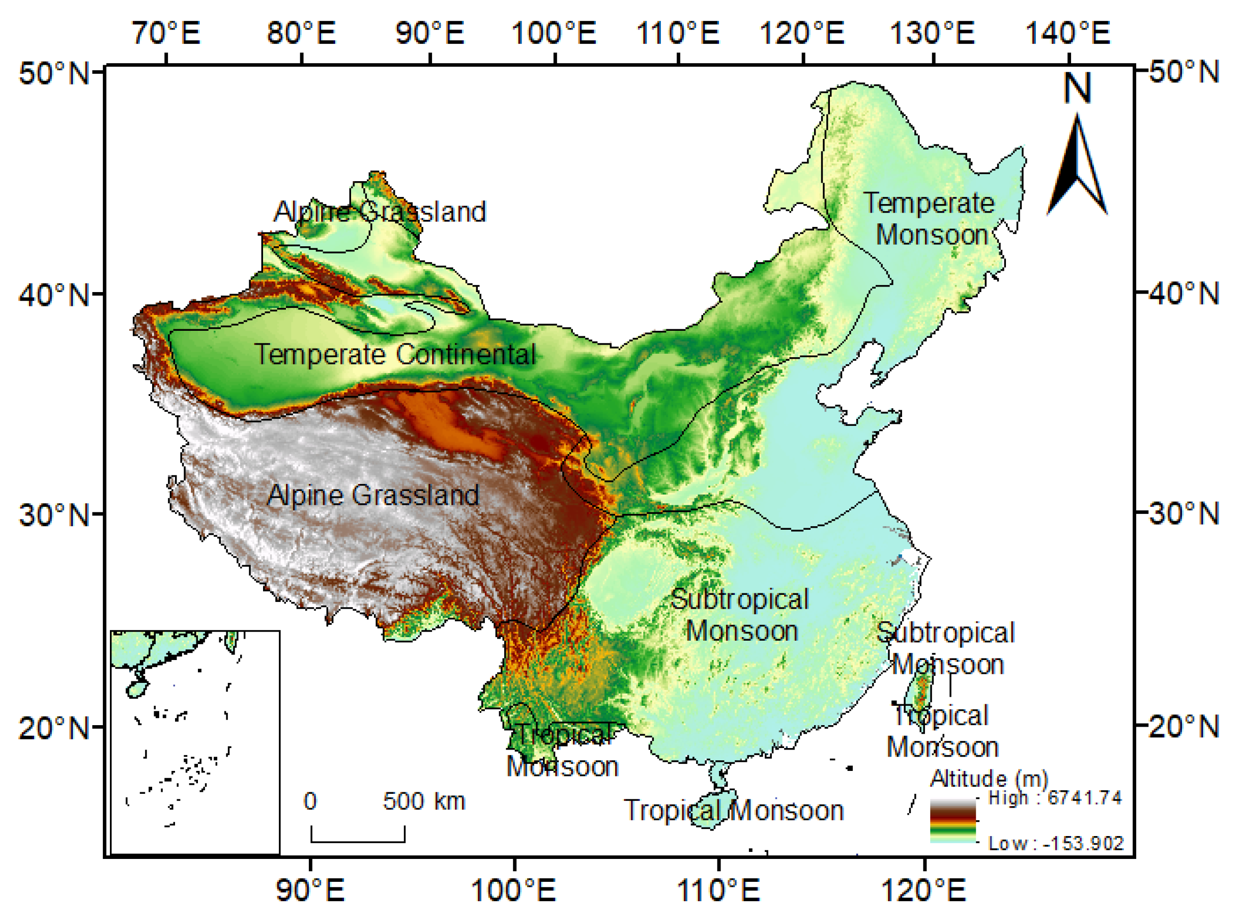
2.1. Study Area

China spans a vast terrain covering 9.6 million square kilometers and boasts a continental coastline spanning 18,000 km in the eastern and southern regions (Figure 1). China’s terrain features a west-to-east gradient. The western territories of the country feature higher elevations, contrasting with the eastern regions, which are characterized by lower elevations, forming a diverse and intricate landscape that resembles a three-stage ladder [10,24]. The country encompasses expansive mountain ranges and plateaus that extend over a significant area. China falls within a diverse array of climates, including tropical monsoon, temperate continental, temperate monsoon, and subtropical monsoon climates. Due to its status as the world’s most populous developing nation, China plays an essential role in the global carbon cycle. The forests, grasslands, agricultural lands, and wetlands serve as vital carbon sinks, efficiently absorbing and sequestering substantial quantities of carbon dioxide [25,26]. In recent years, China has implemented extensive measures to safeguard and bolster these carbon sinks, including large-scale afforestation and wetland conservation [23].

2.2. Data Sources and Processing

2.2.1. NDVI Data

The NDVI dataset utilized in this study was the NOAA/AVHRR NDVI dataset (AVH13C1) spanning the period from 1982 to 2020. This dataset provides gridded daily NDVI derived from the NOAA/AVHRR land surface reflectance product. The spatial resolution of the dataset is 0.05° (~5 km). The data were acquired through the Google Earth Engine (GEE) platform, which is a powerful geospatial and big data analysis platform with large-scale data processing capabilities, providing great convenience for image acquisition and processing of large study areas and long time series [27,28,29]. To mitigate the effects of cloud cover and sensor observation angle, the daily NDVI data were aggregated on a monthly basis, utilizing the maximum value composite (MVC) method. The MVC method improves the quality of monitoring of surface features, especially vegetation, by selecting the maximum value of each pixel point in a series of images to minimize the effects of atmospheric disturbances [30,31]. This approach guarantees enhanced consistency and dataset comparability for the objectives of this research [32].

2.2.2. Meteorological Data

The meteorological data employed were ERA5-Land and TerraClimate datasets. ERA5-Land is a reanalysis dataset that provides numerous land variables spanning several decades at a spatial resolution of 0.1° (~10 km) and has been produced by combining observation data, model data, and remote sensing data using the advanced modelling and data assimilation systems [33]. TerraClimate is a valuable monthly dataset that provides information on climate and water balance. It offers a spatial resolution of 1/24° (~4 km), allowing for a detailed analysis of climatic conditions. From the ERA5-Land dataset, the monthly precipitation and air temperature data were derived, while the TerraClimate dataset provided the monthly solar radiation data. To ensure compatibility with the spatial resolution of the NDVI data, all datasets were resampled to the spatial resolution of 0.05° using a bilinear interpolation method.

2.2.3. Land-Cover Data

The land-cover data utilized in this research were collected from the MODIS land-cover type product (MCD12Q1). This product offers annual land-cover maps with a spatial resolution of 500 m. The land-cover classification was performed using supervised classification methods and MODIS reflectance data. The original MODIS land-cover classification scheme contains 17 types, and these types were merged into 11 categories: evergreen needleleaf forest (ENF), deciduous needleleaf forest (DNF), evergreen broadleaf forest (EBF), deciduous broadleaf forest (DBF), mixed forest (MXF), agricultural land (AL), shrub, grassland, water, bare land, and urban and built-up land (UBL). Then, the reclassified land-cover data were upscaled to 0.05° using the maximum area upscaling method.

2.2.4. DEM Data

The digital elevation model (DEM) data incorporated in this study were derived from the SRTM dataset, which has a spatial resolution of 90 m. To obtain slope and aspect, the elevation data were processed utilizing the Spatial Analyst tool of ArcGIS 10.2. The elevation, slope, and aspect were also resampled to the spatial resolution of 0.05°.

2.2.5. FLUXNET Data

The GPP observation data were obtained from the FLUXNET website (https://www.fluxnet.org/, accessed on 27 September 2023). FLUXNET provides a crucial collection of datasets employed in the examination of global ecosystem carbon, water, and energy cycles. These datasets include a wide array of information, comprising atmospheric greenhouse gas concentrations, soil moisture levels, solar radiation, vegetation growth rates, net ecosystem carbon exchange (NEE), gross primary productivity (GPP), evapotranspiration, photosynthetic rates, as well as an assortment of meteorological parameters. In this study, we selected all Chinese sites in the FLUXNET2015 dataset, ten in total, and excluded the invalid records with the daytime GPP of zero to validate the estimated NPP. The specific information of each flux site is shown in

Table 1. Description of FLUXNET2015 sites in China.

Site ID	Site Name	Period	Latitude	Longitude
CN-Cha	Changbaishan	2003–2005	42.40N	128.10E
CN-Cng	Changling	2007–2010	44.59N	123.51E
CN-Dan	Dangxiong	2004–2005	30.50N	91.07E
CN-Din	Dinghushan	2003–2005	23.17N	112.54E
CN-Du2	Duolun_grassland	2008	42.05N	116.28E
CN-Du3	Duolun Degraded Meadow	2009	42.06N	116.28E
CN-Ha2	Haibei Shrubland	2003–2005	37.61N	101.33E
CN-HaM	Haibei Alpine Tibet site	2002–2004	37.37N	101.18E
CN-Qia	Qianyanzhou	2003–2005	26.74N	115.06E
CN-Sw2	Siziwang Grazed	2011	41.79N	111.90E

. We used the GPP data of the FLUXNET sites and calculated the autotrophic respiration (${\mathrm{R}}_{\mathrm{a}}$) of each site [34,35]. Subsequently, we determined the NPP of each site according to the formula “NPP=GPP-${\mathrm{R}}_{\mathrm{a}}$” to validate the NPP results estimated by the CASA model.

2.3. Research Methods

2.3.1. NPP Estimation

The CASA was employed for the calculation of NPP. The CASA is a model that leverages remote sensing and meteorological data to drive light energy utilization [36]. According to the CASA, NPP is influenced by two primary factors: the light utilization efficiency (LUE) and the absorbed photosynthetically active radiation (APAR) [16,36]:

$$NPP(x,t)=APAR(x,t)\times ϵ(x,t)$$

(1)

where NPP(x, t) is the NPP of pixel x in month t (unit: gC·m⁻²), APAR(x, t) denotes the APAR of pixel x in month t (unit: MJ·m⁻²), and $ϵ(x,t)$ is the actual LUE of pixel x in month t (unit: gC·MJ⁻¹). The calculation of APAR employs the following formula [36]:

$$APAR(x,t)=FPAR(x,t)\times SOL(x,t)\times 0.5$$

(2)

where SOL(x, t) is the total solar radiation (SOL) of pixel x in month t (unit: MJ·m⁻²), and FPAR is the fraction of photosynthetically active radiation (FPAR) of pixel x in month t. FPAR is shown to have a robust linear relationship with NDVI and SR (simple ratio) and can be determined using the following equation:

$$FPAR(x,t)=\alpha FPA{R}_{NDVI}+(1-\alpha )FPA{R}_{SR}$$

(3)

$$FPA{R}_{NDVI}=\frac{NDV{I}_{(x,t)}-NDV{I}_{(i,min)}}{NDV{I}_{(i,max)}-NDV{I}_{(i,min)}}\times (FPR{A}_{max}-FPR{A}_{min})+FPR{A}_{min}$$

(4)

$$FPA{R}_{SR}=\frac{S{R}_{(x,t)}-S{R}_{(i,min)}}{S{R}_{(i,max)}-S{R}_{(i,min)}}\times (FPR{A}_{max}-FPR{A}_{min})+FPR{A}_{min}$$

(5)

$$S{R}_{(x,t)}=\frac{1+NDV{I}_{(x,t)}}{1-NDV{I}_{(x,t)}}$$

(6)

where $\alpha =0.5$, $NDV{I}_{i,min}$ and $NDV{I}_{i,max}$ are the minimum and maximum values of NDVI of vegetation type i, respectively. $FPA{R}_{min}$ and $FPA{R}_{max}$ are constants with the values of 0.001 and 0.95, respectively. $S{R}_{i,min}$ and $S{R}_{i,max}$ are the minimum and maximum values of SR of vegetation type i, respectively. In

Table 2. The maximum and minimum values of NDVI and SR for each land-cover type, along with the maximum light energy utilization (${\epsilon }_{\max }$) and soil organic carbon density (SOCD).

Code	Land-Cover Type	NDVImax	NDVImin	SRmax	SRmin	$\mathsf{\epsilon }$${}_{\mathbf{max}}$	SOCD (kg·m−2)
1	ENF	0.647	0.023	4.67	1.05	0.389	3.77
2	EBF	0.676	0.023	5.17	1.05	0.985	4.70
3	DNF	0.738	0.023	6.63	1.05	0.485	3.77
4	DBF	0.747	0.023	6.91	1.05	0.692	4.70
5	MXF	0.702	0.023	5.84	1.05	0.475	4.24
6	Shrubland	0.636	0.023	4.49	1.05	0.429	2.56
7	Grassland	0.634	0.023	4.46	1.05	0.542	1.82
8	AL	0.634	0.023	4.46	1.05	0.542	2.56
9	Water	0.634	0.023	4.46	1.05	0.542	0
10	UBL	0.634	0.023	4.46	1.05	0.542	0
11	Bare Land	0.634	0.023	4.46	1.05	0.542	0

, the maximum and minimum values of NDVI and SR are provided for various vegetation types in China [37].

The calculation of LUE ($\epsilon$) is determined using the following equation:

$$\epsilon (x,t)=T_{\epsilon 1}(x,t)\times T_{\epsilon 2}(x,t)\times W_{\epsilon }(x,t)\times {\epsilon }_{max}$$

(7)

where $T_{\epsilon 1}$ represents the stress effect of low temperature on light utilization efficiency, while $T_{\epsilon 2}$ symbolizes the high-temperature stress effect on the same. $W_{\epsilon }$ signifies the coefficient quantifying the repercussion of water stress on light utilization efficiency. ${\epsilon }_{max}$ corresponds to the maximum LUE that can be achieved under optimum conditions (unit: gC·MJ⁻¹). The ${\epsilon }_{max}$ values for typical vegetation types are outlined in Table 2 [37].

2.3.2. NEP Calculation

NEP is determined as follows:

$$NEP=NPP-R_H$$

(8)

The GSMSR was used to estimate monthly soil respiration $R_S$). This model is driven by SOCD, monthly precipitation (unit: mm), and monthly temperature (unit: °C) [38]:

$$R_S=\left(R_{D_{s=0}}+M\times D_s\right)\times e^{ln\alpha e^{\beta T}T/10}\times \left(P+P_0\right)/(P+K)$$

(9)

where $R_{D_{s=0}}$ = 0.588 (unit: gC·m⁻²), $M=0.118$, $\alpha =1.830$, $\beta =-0.006$, $P_0=2.972$, $K=5.657$, P is the monthly precipitation, and T is the monthly average temperature.

The empirical equation utilized $\mathrm{R}\mathrm{S}$ as the input variable to calculate $\mathrm{R}\mathrm{H}$ [10]:

$$R_H=-0.0009R_S^2+0.6011R_S+4.8874$$

(10)

2.3.3. Spatiotemporal Variations

The Theil–Sen median method, a robust non-parametric statistical approach, was employed to measure the temporal evolution trend of NEP. This method is frequently applied in trend analysis of long time series data, offering particular utility in discerning trends amid outliers or non-normal data distributions [39,40]. The Sen slope is calculated using the following formula:

$$\beta =Median\left(\frac{NE{P}_j-NE{P}_i}{j-i}\right)1982\le i<j\le 2020$$

(11)

where $\beta$ denotes the slope, whereas $NE{P}_i$ and $NE{P}_j$ symbolize the NEP values for years i and j, respectively. The Sen slope ($\beta$) indicates the trend degree. An increasing trend is suggested by $\beta >0$, while $\beta <0$ signifies a decreasing trend in the time series.

The Mann–Kendall (MK) test, known for its lower sensitivity to outliers and independence from specific sample distributions, was employed to assess the significance of the NEP trend [41]. The calculation of the test statistic S value is executed as follows:

$$S=\sum _{i=1}^{n-1}\sum _{j=i+1}^{n}sgn(NE{P}_j-NE{P}_i)$$

(12)

$$sgn\left(NE{P}_j-NE{P}_i\right)=\left\{\begin{array}{cc}\hfill 1& NE{P}_j-NE{P}_i>0\\ \hfill 0& NE{P}_j-NE{P}_i=0\\ \hfill -1& NE{P}_j-NE{P}_i<0\end{array}\right.$$

(13)

The calculation of the test statistic Z value by standardized S was as follows:

$$Z=\left\{\begin{array}{cc}\frac{S-1}{\sqrt{var\left(S\right)}}\hfill & S>0\hfill \\ 0\hfill & S=0\hfill \\ \frac{S+1}{\sqrt{var\left(S\right)}}\hfill & S<0\hfill \end{array}\right.$$

(14)

$$var\left(S\right)=\frac{n(n-1)(2n+5)-{\sum }_{i=1}^m{t}_i(t_i-1)(2t_i+5)}{18}$$

(15)

where n is the number of samples in the sequence, m denotes the number of groups within the sequence that contain repetitive data, and $t_i$ stands for the count of repeated data points within group i.

A two-tailed trend test allows the critical values $Z_{1-\alpha /2}$ to be obtained from the standard normal distribution table at a specified significance level. If $\left|Z\right|\le Z_{1-\alpha /2}$, we accept the null hypothesis. Conversely, when $\left|Z\right|>Z_{1-\alpha /2}$, the null hypothesis is rejected, indicating a significant trend. Significance levels of $\alpha =0.05$ and $\alpha =0.01$ were adopted in this study, and the corresponding critical values were $Z_{1-\alpha /2}=\pm 1.96$ and $Z_{1-\alpha /2}=\pm 2.58$, respectively.

2.3.4. Geodetector Model

The Geodetector model was employed to examine the connections between the NEP change rate and various environmental factors. The Geodetector method, a novel statistical approach, is utilized for detecting spatial variations and uncovering the underlying driving factors [42]. The factor detection module and interaction detection module of the geographical detector model were applied to explore the strength of individual factor effects and the strength of interaction effects between pairs of factors.

The q-value calculation was carried out to understand how significantly an environmental factor elucidates the spatial divergence of attribute Y. The formula utilized for determining the q-value is given below [42]:

$$q=1-\frac{SSW}{SST}=1-\frac{{\sum }_{h=1}^L{N}_h{{\sigma }_h}^2}{N{\sigma }^2}$$

(16)

where SST and SSW are the total sum of squares and the within sum of squares, respectively. $h=1,\dots ,L$ corresponds to the strata or divisions of the factor X. The symbols $N_h$ and N represent the quantity of units within a given stratum h and the cumulative units, respectively. Similarly, ${\sigma }_h^2$ and ${\sigma }^2$ are indicative of the variances of Y within a specific stratum h and across the entire region, respectively. The q value ranges between 0 and 1. A higher value of q signifies a strong explanatory power of the independent variable X over the dependent variable Y. Conversely, a lower q value indicates a weaker explanatory degree.

We use the detection of interaction factors to identify the interplay among various risk factors, denoted as $X_s$. This specifically enables us to measure whether the combined influence of factors $X_1$ and $X_2$ enhances or reduces the explanatory power of the dependent variable Y. Furthermore, this method helps to evaluate whether these factors have an independent impact on Y. A comprehensive outline of interaction types is shown in

Table 3. Interaction types of driving factors in the Geodetector model.

Relations of q-Value	Type of Interaction
$q(X1\cap X2)<min\left(q\right(X1),q(X2\left)\right)$	Nonlinear weakened
$min\left(q\right(X1),q(X2\left)\right)<q(X1\cap X2)<max\left(q\right(X1),q(X2\left)\right)$	Single factor nonlinear weakened
$q(X1\cap X2)>max\left(q\right(X1),q(X2\left)\right)$	Bivariable enhanced
$q(X1\cap X2)=q\left(X1\right)+q\left(X2\right)$	Independent
$q(X1\cap X2)>q\left(X1\right)+q\left(X2\right)$	Nonlinear enhanced

.

Six environmental factors were selected to analyze their relationship with the NEP change rate, namely precipitation change rate, solar radiation change rate, temperature change rate, altitude, aspect, and slope. As the Geodetector algorithm operates on discrete data, the six continuous independent variables were transformed into discrete categories using an optimal method [42]. The “GD” package available in the R Studio software was used for the classification procedure [43]. The slope was classified using the quantile method, and the remaining independent variables were classified using the natural breaks method. The reclassified factors are illustrated spatially in Figure 2.

3. Results

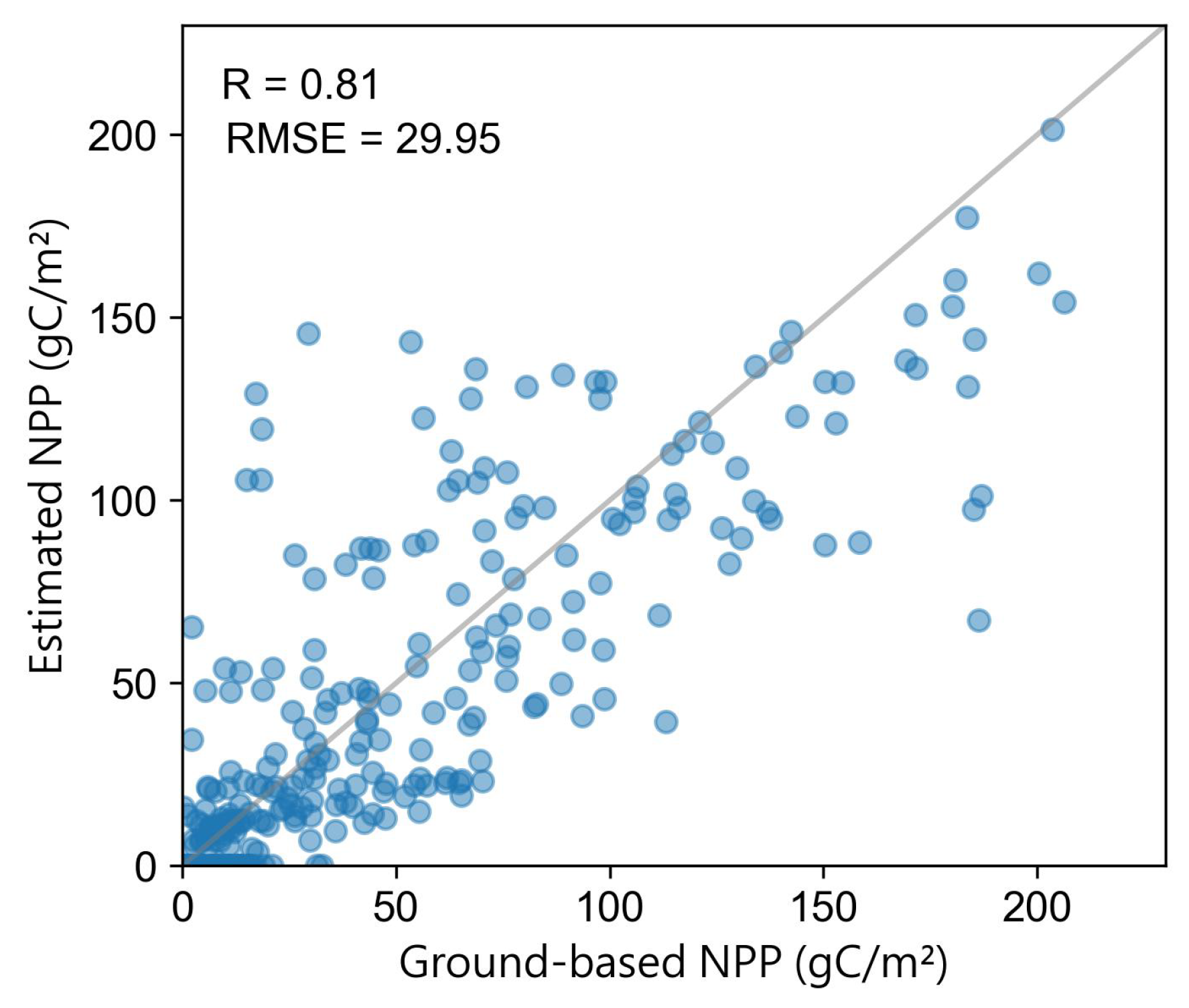
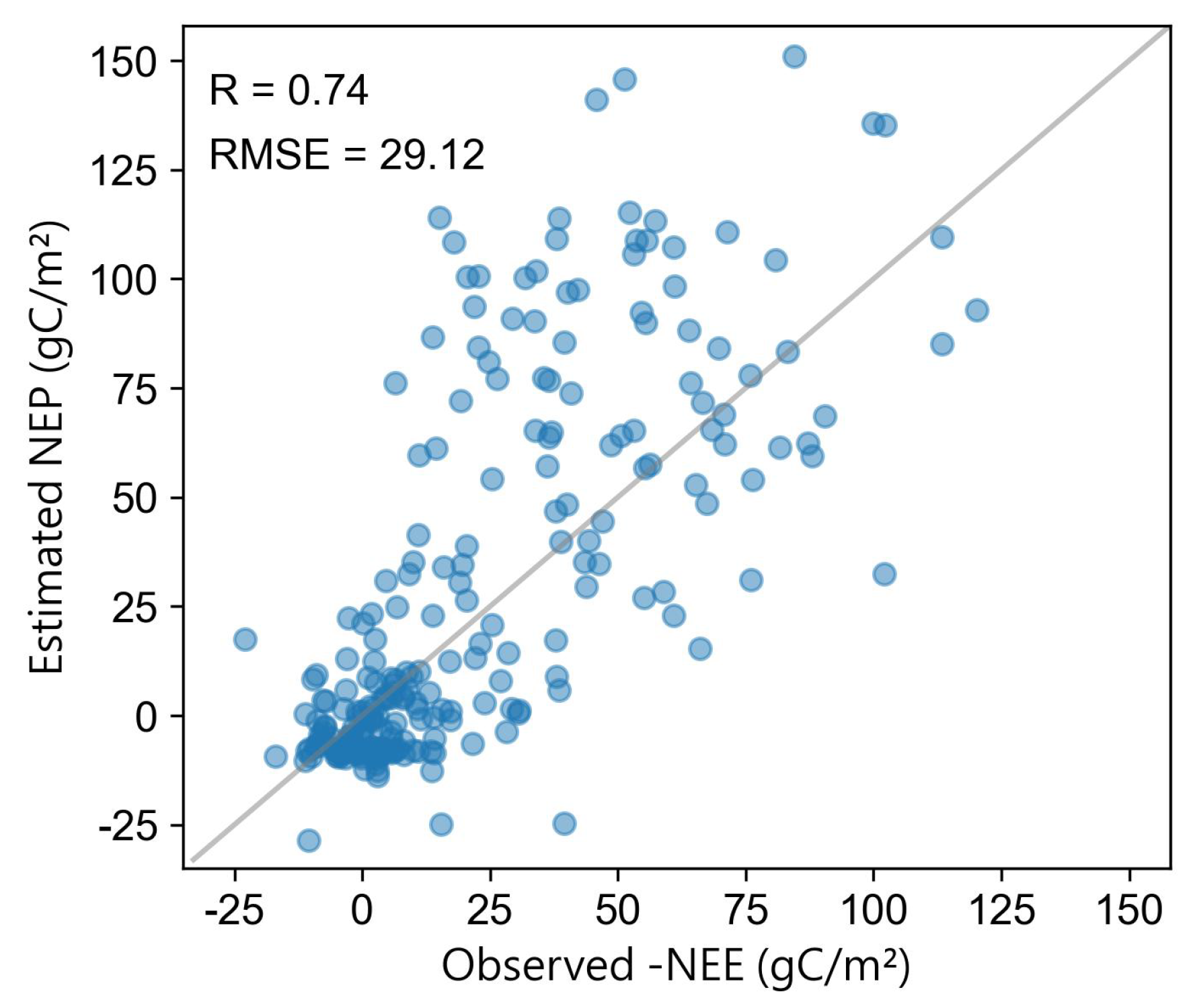
3.1. NPP and NEP Validation

The modeled NPP values using remotely sensed data in the corresponding FLUXNET sites were derived based on the latitude and longitude coordinates of the flux sites and then compared with the calculated NPP results from the FLUXNET database (Figure 3). The root mean square error (RMSE) and the correlation coefficient (R) were calculated to indicate the estimation accuracy. Most of the sample points clustered near the 1:1 line, with an RMSE of 29.95 gC·m⁻² and an R of 0.81. Moreover, this is consistent with the simulation results of Guo et al. [9] and Ji et al. [44] in terms of accuracy, which suggests that the estimated NPP has a good degree of accuracy.

We also validated the estimated NEP results. We approximated the ground actual observed NEP by taking the negative values of Net Ecosystem Exchange (NEE) observed at Fluxnet sites (Figure 4). We compared this approximation with NEP estimated based on remote sensing at corresponding times and locations to assess the accuracy of our NEP estimates. The results indicated a correlation coefficient (R) of 0.74 and a root mean square error (RMSE) of 29.12 gC·m⁻². Our findings demonstrate good accuracy in the estimated NEP results.

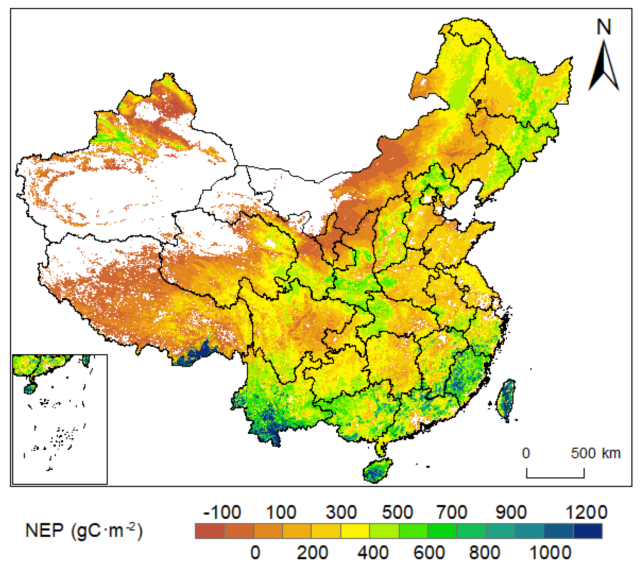
3.2. Spatial Distribution of NEP

Figure 5 shows the 39-year NEP averages during 1982–2020 in China. NEP exhibits an obvious spatial pattern, and it was observed that NEP was generally lower in the northern regions and higher in the southern regions. Similarly, NEP exhibited a lower value in the western areas compared to the eastern regions. The mean NEP value of China during the 39-year period was 265.38 gC·m⁻², indicating a significant carbon sink. The annual average carbon sequestration amounted to 1.89 PgC. During 1982–2020, the vegetation area in China that showed a carbon sink effect was 8,462,600 km², accounting for 88.18% of the total vegetation area. This area showed a carbon source effect of 1,134,400 km², covering 11.82% of the vegetation area.

The mean annual NEP value exceeds 400 gC·m⁻² in northeastern, southwestern, and southeastern China. Among these regions, high NEP values (>1000 gC·m⁻²) were observed in the Southeastern Tibetan Plateau, Southern Sichuan, Hainan, Taiwan, and Fujian Province. Most of these areas are characterized by low topography, warm climate, and abundant precipitation, making them highly suitable for vegetation growth. Conversely, most areas in the Tibetan Plateau, Xinjiang, and Inner Mongolia that are controlled by arid or semi-arid climate showed much lower NEP values, generally less than 100 gC·m⁻² or even negative.

3.3. Spatiotemporal Variations in NEP

The annual average vegetation NEP of China showed a fluctuating increasing trend during 1982–2020 (Figure 6a). The overall average increasing rate is 4.69 gC·m⁻²·a⁻¹. Over this period, NEP showed a general pattern of increasing–decreasing–increasing–decreasing–increasing. The lowest annual average NEP occurred in 1982 at 174.99 gC·m⁻², and the peak value was recorded in 2015 at 396.68 gC·m⁻².

The seasonal variation of NEP was also analyzed. Figure 6b shows the temporal curve of monthly mean vegetation NEP. It exhibited an obvious unimodal characteristic, ranging from −2.79 to 69.99 gC·m⁻². The peak NEP value was observed in July at 39.81 gC·m⁻², while the minimum NEP value of −2.79 gC·m⁻² was observed in February. From March to November, the monthly NEP is higher than 0, indicating that the vegetation ecosystem in China acted as a carbon sink during these months. From December to February, the monthly NEP was lower than 0, suggesting that the vegetation ecosystem in China served as a carbon source.

We applied the Theil–Sen method to the estimated annual NEP data, resulting in the spatial distribution of vegetation NEP trends during 1982–2020 (Figure 7). During this interval, an increasing trend was evident across the majority of the vegetated area. The area with increasing trends covered 8,856,424 km², covering 93.45% of the total vegetation region. Within these regions, approximately 33.87% had change rates below 3 gC·m⁻²·a⁻¹, which were mostly located in northwest China, the Tibetan Plateau, and northeast China. About 18.14% of the vegetation area exhibited NEP growth rates between 3 and 5 gC·m⁻²·a⁻¹, while 32.43% showed growth rates between 5 and 10 gC·m⁻²·a⁻¹. These higher growth rates were predominantly distributed in China’s eastern and southern regions. Furthermore, 8.24% of the vegetation area displayed NEP growth rates between 10 and 20 gC·m⁻²·a⁻¹, with only 0.77% exhibiting growth rates exceeding 20 gC·m⁻²·a⁻¹. These areas were concentrated in southwest China, Hainan, and Taiwan, suggesting that the carbon sink effect in these areas increased considerably over the past four decades.

Conversely, an area of 620.755 km² exhibited decreasing trends in NEP, covering 6.55% of the total vegetation area. Approximately 88.88% of the vegetation area exhibited a decrease rate below 3 gC·m⁻²·a⁻¹, indicating a significant portion of the vegetation exhibiting declining NEP rates. These areas are primarily situated in the Tibetan Plateau and northwest China. Additionally, 5.19% showed decline rates between 3 and 5 gC·m⁻²·a⁻¹, 3.58% between 5 and 10 gC·m⁻²·a⁻¹, and only 2.34% exhibited decline rates exceeding 10 gC·m⁻²·a⁻¹, which were dispersed throughout the national territory.

Figure 8 shows the distribution of the significance level of the trend over China during 1982–2020. The vast majority of the vegetation region in China exhibited significant increasing trends in NEP (significant increase and mild increase), accounting for 71% of the vegetation region. Additionally, there was a significant increase of 7.07%. The areas with insignificant changes in vegetation NEP in the study area accounted for 20.16% of the total vegetation region. Among them, 14.97% did not increase significantly, and 5.18% did not decrease significantly. The areas primarily exhibiting no significant reductions were situated in Inner Mongolia and the Tibetan Plateau. The areas with slightly decreased and significantly decreased trends accounted for only 0.6% and 0.74% of the vegetation region, respectively, and were sporadically distributed. Overall, the majority of the vegetation region in China exhibited a significant increasing trend during 1982–2020. This indicates a positive evolution of vegetation in China, suggesting an increase in its carbon sink capacity.

3.4. Driving Factors in NEP Variation

The factor detector in the Geodetector model was used to analyze the impacts of six factors (precipitation change rate, temperature change rate, solar radiation change rate, altitude, aspect, and slope) on the NEP change rate. All six environmental factors influenced the spatial variability of the NEP change rate at a statistically significant level ($p<0.01$). Among them, the precipitation change rate had the strongest effect (q-value = 0.198). This was followed by solar radiation change rate (0.124) and altitude (0.122) (Figure 9a), suggesting that these three factors played a significant role in influencing the temporal change of NEP in China. Precipitation directly affects the amount of water available to plants. Moisture is a key limiting factor for plant photosynthesis and growth. Adequate precipitation can increase soil moisture, thereby increasing the rate of photosynthesis and growth of plants. On the other hand, insufficient or excessive precipitation can adversely affect plants. Drought conditions can limit plant photosynthesis, while excessive precipitation may lead to water stress, affecting the availability of oxygen to the roots [45,46]. This is also consistent with previous research [13,47,48,49,50]. Slope, temperature change rate, and aspect had weak effects on NEP change, as evidenced by their lower q-values of 0.021, 0.017, and 0.007, respectively.

The Geodetector model’s interaction detector was employed to examine how the interaction between two significant factors influences changes in the NEP. Figure 9b shows the q-statistic values of each pair of the six driving factors. The results revealed that the paired factors had noticeably larger q-statistics compared to the individual q-statistics (Figure 9b). The interaction between the precipitation change rate and altitude has the largest effect, with a q-statistic value of 0.29, indicating that precipitation and altitude are the main factors influencing NEP temporal change. This is similar to previous findings [50,51,52]. At lower altitudes, an increase in NEP is observed, likely due to enhanced precipitation levels that favor plant growth and ecosystem productivity. Conversely, at higher altitudes, a decline in NEP is noted, attributable to the reduced temperature and precipitation, which are less conducive to sustaining high levels of ecosystem productivity. In addition, the q-values of the interactions between precipitation, solar radiation, temperature, slope, and aspect were larger than those of the other factors, all with q-values greater than 0.2, indicating that the interactions between precipitation and various other factors have a more pronounced impact on the changes in NEP under the effect of the precipitation change rate as the main influencing factor. Among all the interaction pairs, four pairs are bilinearly strengthened (solar radiation change rate and precipitation change rate, precipitation change rate and elevation, precipitation change rate and slope direction, solar radiation change rate and elevation), and the others are unilinearly strengthened. The interactions of the drivers of the NEP change rate are all enhancing effects, and there are no factors that act independently of each other.

4. Discussion

NEP contributes to the understanding of vegetation carbon sources and sinks and holds significant importance for studying the carbon cycle [1,53]. Numerous research efforts have been undertaken to explore the spatial and temporal changes in NEP using remote sensing techniques. However, most of the studies were based on MODIS remote sensing data [11,12,44,54]. MODIS data have been available since 2000, limiting the examination of carbon source/sink dynamics over extended temporal periods. This study derived NEP from NOAA/AVHRR remote sensing data, which have been available since 1981 and provided a much longer temporal coverage than MODIS data. In addition, previous studies on NEP primarily concentrate on smaller regional scales or specific provincial and regional units [11,12,44]. This study took China as the study area, covering a large area with various climates and vegetation zones. Being one of the world’s most populous countries, China also plays a substantial role in the global carbon cycle [25,26]. This research investigated the spatiotemporal variations in NEP in China during 1982–2020, providing meaningful knowledge of the fundamental carbon balance.

In this study, we compared the NPP calculation results obtained from the CASA estimation with the actual measurements of FLUXNET sites (Figure 3). Our findings indicate a good level of consistency between the two datasets, with a good fitting accuracy, characterized by the correlation coefficient (R) of 0.81. These results confirm the good accuracy of the NPP estimated in this work. In addition, the GSMSR was used to estimate the soil respiration ${\mathrm{R}}_{\mathrm{H}}$ in this study. Moreover, Liang et al. [10] and Shi [55] also used the same soil respiration model estimation method to estimate the monthly ${\mathrm{R}}_{\mathrm{H}}$ in the China region and Shanxi Province, respectively, and used it to calculate the NEP. They demonstrated that the results of this model estimation were reliable by validating the results of the NEP estimation. We validated the estimated NEP using the NEE observed at the FLUXNET sites. The correlation coefficient (R) between the two sets of values is 0.74 and the root mean square error (RMSE) is 29.12. From Figure 4, it can be observed that the NEP values are slightly overestimated. However, it should be noted that the value of NEP cannot simply be regarded as the opposite of NEE. NEE represents the net exchange of carbon dioxide with the atmosphere, encompassing both vertical and lateral carbon fluxes between ecosystems and the atmosphere. When the atmosphere is highly stable or there is strong soil carbon respiration leading to minimal flux, NEE approaches NEP (but with opposite signs) [56,57]. Therefore, using NEE as the reference may introduce some uncertainties in the validation. Due to the different research methods, data sources, and time scales used in different studies, the NEP estimation results have some differences. Yao et al. [58] obtained an average NEP value of 1.18 ± 0.05 PgC ·a⁻¹ for China from 2000 to 2015 by employing the model tree ensemble approach. However, the estimation results of Wang et al. [59] are very similar to ours. Wang et al. [59] used the eddy covariance measurement method and obtained a value of 1.89 PgC·a⁻¹ for China’s NEP for the years 2001–2010. Additionally, the research by Liu et al. [18] utilized GPP data from AVHRR to calculate China’s NEP from 1982 to 2018, estimating the result to be 1.4–1.6 PgC·a⁻¹. Zhu et al. [60] developed a statistical assessment scheme, estimating China’s NEP for the 2000s to be 1.91 ± 0.15 PgC·a⁻¹. Compared with previous studies, the NEP estimation results of this paper are within the reliable range, further indicating their high degree of accuracy.

China’s diverse climate types and complex terrain contribute to the formation of intricate terrestrial ecosystems, influencing changes in vegetation carbon sources and sinks [10,24]. Investigating the effect of climate and natural factors on the vegetation NEP temporal change in China can help develop strategies and management measures to address climate change. Previous studies predominantly used correlation analysis to examine the relationship between NEP and climate factors, with limited attention given to topographic factors (e.g., altitude, slope, and aspect). These studies primarily focus on the isolated impacts of driving factors [44], making it challenging to evaluate the interactions among these factors. This study employed the Geodetector method to detect the impact of climatic and topographic factors in NEP change. Compared with the correlation method, the Geodetector approach has several advantages, including not being affected by multicollinearity issues, effectively quantifying the combined driving effects of single and multiple factors in geographic phenomena, and revealing whether the interplay between two factors follows a linear or non-linear trend [42]. However, geospatial analysis also has the limitation that it can only investigate the effects of the spatial distribution of independent variables on the dependent variable [61]. In this study, we used the Sen slope of NEP and meteorological factors as the input variables to explore the interaction between factors that influenced the temporal change in NEP based on the spatial distribution of the change rate. The results demonstrate that the precipitation change rate exerted the most significant influence on NEP change (q-value = 0.1982). This is consistent with the studies of others [13,47,48,49,50]. Photosynthesis and overall growth of plants are highly dependent on water. When precipitation levels are optimal, it helps to increase soil moisture, which benefits photosynthesis and promotes plant growth. On the other hand, drought or excessive rainfall can have a detrimental effect. Limited rainfall can hinder the photosynthesis process due to water scarcity, while too much rainfall can lead to saturation, which can create challenges for oxygen supply to the roots [45,46]. It is noteworthy that the results of the Geodetector method indicate that precipitation is the primary driving factor influencing changes in NEP. This suggests that in most regions, precipitation plays a crucial role in driving changes in NEP. However, due to the vast geographical expanse, complex topography, and diverse climatic conditions in China, the overall trend of precipitation may not necessarily align with changes in NEP in Chinese vegetation regions. In addition, the results of the cross-test showed that the q-values of the paired factors exceeded the q-values of the individual factors. The interaction between precipitation rate of change and elevation had the largest effect, with a q-statistic of 0.29, indicating that precipitation and elevation were the main factors influencing temporal variation in NEP. This observation is similar to previous studies [50,51,52]. At lower elevations, NEP increases with elevation due to increased precipitation, but at higher elevations, NEP decreases with elevation due to decreased temperature and precipitation.

This study also has some limitations. The land cover used in this study is the MODIS land-cover product, which has been valid since 2000. Therefore, land-cover data prior to 2020 are considered to be the same as in 2000. Moreover, anthropogenic factors (e.g., GDP, human activity intensity, population density, and land use type) also have a remarkable influence on vegetation NEP [11,62]. However, due to the unavailability of anthropogenic factor data spanning from 1982 to the present, their change rates could not be calculated, and thus, their effects were not considered in this research.

5. Conclusions

Based on the CASA and GSMSR, this study examined the spatiotemporal variations in NEP in China from 1982 to 2020 by integrating reanalysis meteorological data and satellite data. The interactive and relative contributions of climatic and topographic factors of NEP changes during the 39 years were also analyzed using the Geodetector model. The main conclusions are as follows:

(1)

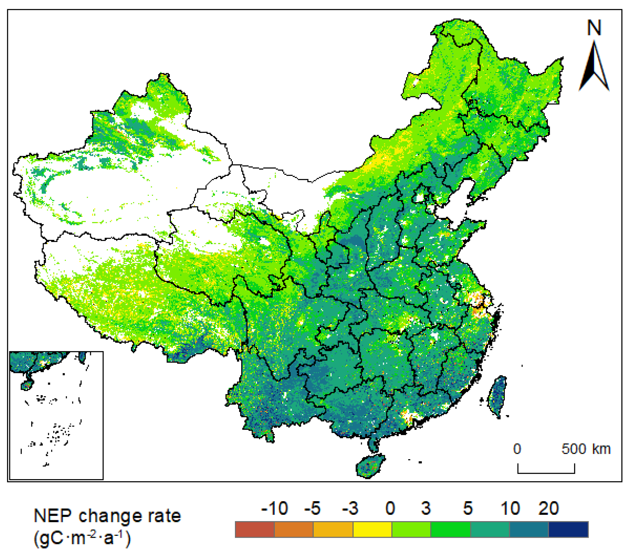
The study revealed a distinct spatial distribution pattern of vegetation NEP in China. It was observed that NEP was generally lower in the northern regions and higher in the southern regions. Similarly, NEP was lower in the western areas than that in the eastern regions. The mean NEP of the study region over 39 years was 265.38 gC·m⁻². The annual average carbon sequestration amounted to 1.89 PgC, indicating a large carbon sink.

(2)

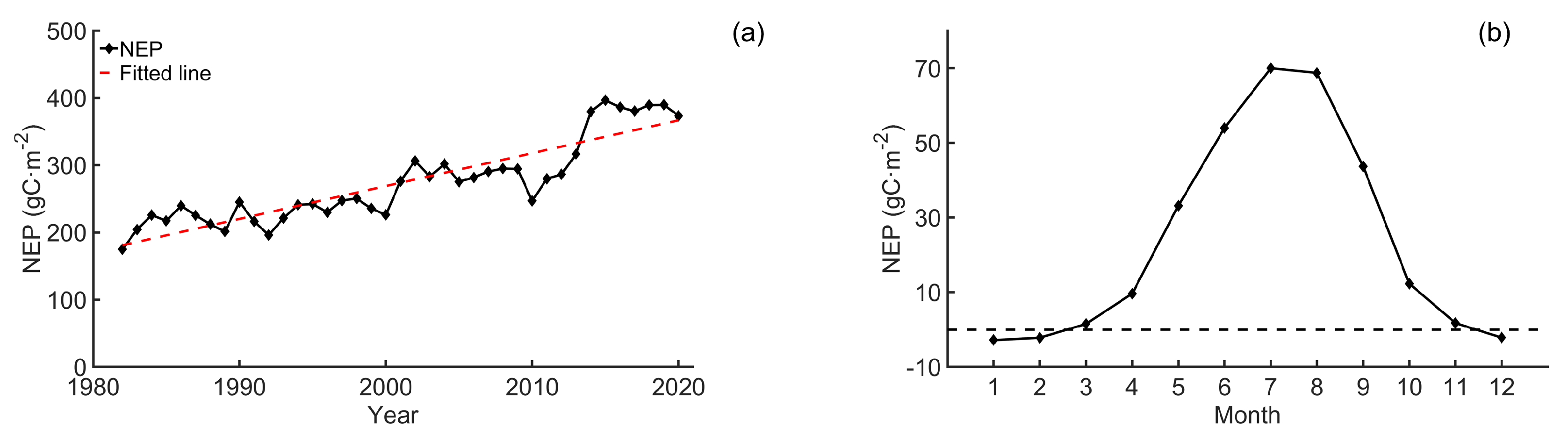
During 1982–2020, the annual mean NEP of the Chinese vegetation region exhibited a general fluctuating upward trend. In terms of NEP seasonal change, the vegetation area in China was generally a carbon sink from March to November, and a carbon source from December to February. During the 39-year period, a significant proportion of vegetated regions in China showed an upward trend in NEP, and the overall average growth rate in China’s vegetation areas is 4.69 gC·m⁻²·a⁻¹. This indicates an enhanced carbon sequestration capacity of these vegetated regions.

(3)

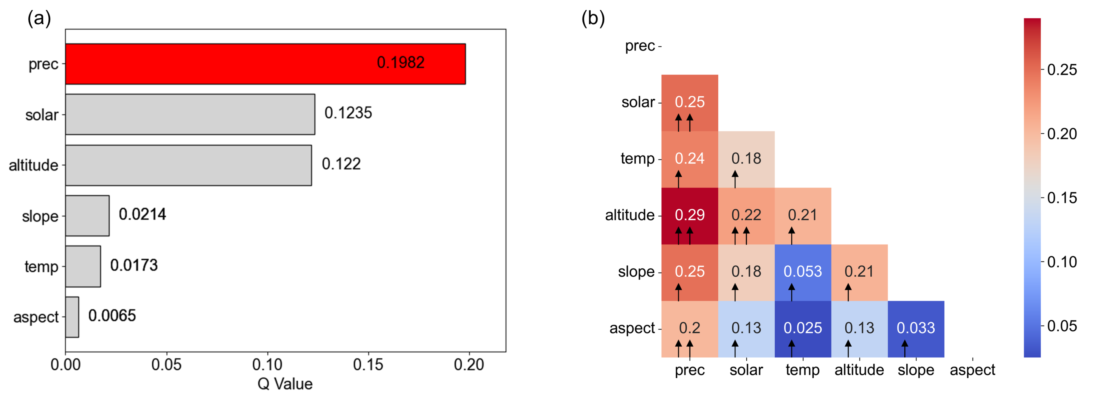
Precipitation, solar radiation, and altitude are the key driving forces on the temporal change in NEP among the climatic and topographic factors. The interactions between the driving factors showed significantly higher impacts on NEP change than the single factor. The interaction between precipitation rate and elevation has the strongest effect, with the q-statistic value of 0.29.

References

1. Pathak, K.; Malhi, Y.; Sileshi, G.; Das, A.K.; Nath, A.J. Net ecosystem productivity and carbon dynamics of the traditionally managed Imperata grasslands of North East India. Sci. Total. Environ. 2018, 635, 1124–1131. [Google Scholar] [CrossRef] [PubMed]
2. Schimel, D.; Stephens, B.B.; Fisher, J.B. Effect of increasing CO2 on the terrestrial carbon cycle. Proc. Natl. Acad. Sci. USA 2015, 112, 436–441. [Google Scholar] [CrossRef] [PubMed]
3. Friend, A.D.; Lucht, W.; Rademacher, T.T.; Keribin, R.; Betts, R.; Cadule, P.; Ciais, P.; Clark, D.B.; Dankers, R.; Falloon, P.D.; et al. Carbon residence time dominates uncertainty in terrestrial vegetation responses to future climate and atmospheric CO2. Proc. Natl. Acad. Sci. USA 2014, 111, 3280–3285. [Google Scholar] [CrossRef] [PubMed]
4. Bloom, A.A.; Exbrayat, J.F.; Van Der Velde, I.R.; Feng, L.; Williams, M. The decadal state of the terrestrial carbon cycle: Global retrievals of terrestrial carbon allocation, pools, and residence times. Proc. Natl. Acad. Sci. USA 2016, 113, 1285–1290. [Google Scholar] [CrossRef] [PubMed]
5. Zhang, J.; Hao, X.; Hao, H.; Fan, X.; Li, Y. Climate change decreased net ecosystem productivity in the arid region of central Asia. Remote Sens. 2021, 13, 4449. [Google Scholar] [CrossRef]
6. Ge, W.; Deng, L.; Wang, F.; Han, J. Quantifying the contributions of human activities and climate change to vegetation net primary productivity dynamics in China from 2001 to 2016. Sci. Total. Environ. 2021, 773, 145648. [Google Scholar] [CrossRef] [PubMed]
7. IGBP Terrestrial Carbon Working Group; Steffen, W.; Noble, I.; Canadell, J.; Apps, M.; Schulze, E.D.; Jarvis, P.G. The terrestrial carbon cycle: Implications for the Kyoto Protocol. Science 1998, 280, 1393–1394. [Google Scholar]
8. Ruimy, A.; Saugier, B.; Dedieu, G. Methodology for the estimation of terrestrial net primary production from remotely sensed data. J. Geophys. Res. Atmos. 1994, 99, 5263–5283. [Google Scholar] [CrossRef]
9. Guo, D.; Song, X.; Hu, R.; Zhu, X.; Jiang, Y.; Cai, S.; Zhang, Y.; Cui, X. Large-scale analysis of the spatiotemporal changes of Net Ecosystem Production in Hindu Kush Himalayan Region. Remote Sens. 2021, 13, 1180. [Google Scholar] [CrossRef]
10. Liang, L.; Geng, D.; Yan, J.; Qiu, S.; Shi, Y.; Wang, S.; Wang, L.; Zhang, L.; Kang, J. Remote sensing estimation and spatiotemporal pattern analysis of terrestrial net ecosystem productivity in China. Remote Sens. 2022, 14, 1902. [Google Scholar] [CrossRef]
11. Wang, C.; Zhao, W.; Zhang, Y. The Change in Net Ecosystem Productivity and its Driving Mechanism in a Mountain Ecosystem of Arid Regions, Northwest China. Remote Sens. 2022, 14, 4046. [Google Scholar] [CrossRef]
12. Lu, X.; Chen, Y.; Sun, Y.; Xu, Y.; Xin, Y.; Mo, Y. Spatial and temporal variations of net ecosystem productivity in Xinjiang Autonomous Region, China based on remote sensing. Front. Plant Sci. 2023, 14, 1146388. [Google Scholar] [CrossRef] [PubMed]
13. Feng, X.; Fan, Q.; Qu, J.; Ding, X.; Niu, Z. Characteristics of carbon sources and sinks and their relationships with climate factors during the desertification reversal process in Yulin, China. Front. For. Glob. Chang. 2023, 6, 1288449. [Google Scholar] [CrossRef]
14. Ran, Y.; Li, X.; Sun, R.; Kljun, N.; Zhang, L.; Wang, X.; Zhu, G. Spatial representativeness and uncertainty of eddy covariance carbon flux measurements for upscaling net ecosystem productivity to the grid scale. Agric. For. Meteorol. 2016, 230, 114–127. [Google Scholar] [CrossRef]
15. Zhang, K.; Zhu, C.; Ma, X.; Zhang, X.; Yang, D.; Shao, Y. Spatiotemporal Variation Characteristics and Dynamic Persistence Analysis of Carbon Sources/Sinks in the Yellow River Basin. Remote Sens. 2023, 15, 323. [Google Scholar] [CrossRef]
16. Field, C.B.; Randerson, J.T.; Malmström, C.M. Global net primary production: Combining ecology and remote sensing. Remote Sens. Environ. 1995, 51, 74–88. [Google Scholar] [CrossRef]
17. Huang, C.; Sun, C.; Nguyen, M.; Wu, Q.; He, C.; Yang, H.; Tu, P.; Hong, S. Spatio-temporal dynamics of terrestrial Net ecosystem productivity in the ASEAN from 2001 to 2020 based on remote sensing and improved CASA model. Ecol. Indic. 2023, 154, 110920. [Google Scholar] [CrossRef]
18. Liu, M.; Bai, X.; Tan, Q.; Luo, G.; Zhao, C.; Wu, L.; Chen, F.; Li, C.; Yang, Y.; Ran, C.; et al. Climate change enhanced the positive contribution of human activities to net ecosystem productivity from 1983 to 2018. Front. Ecol. Evol. 2023, 10, 1101135. [Google Scholar] [CrossRef]
19. Pei, Z.Y.; Ouyang, H.; Zhou, C.P.; Xu, X.L. Carbon Balance in an Alpine Steppe in the Qinghai-Tibet Plateau. J. Integr. Plant Biol. 2009, 51, 521–526. [Google Scholar] [CrossRef]
20. Parton, W.; Morgan, J.; Smith, D.; Del Grosso, S.; Prihodko, L.; LeCain, D.; Kelly, R.; Lutz, S. Impact of precipitation dynamics on net ecosystem productivity. Glob. Chang. Biol. 2012, 18, 915–927. [Google Scholar] [CrossRef]
21. Liang, W.; Yang, Y.; Fan, D.; Guan, H.; Zhang, T.; Long, D.; Zhou, Y.; Bai, D. Analysis of spatial and temporal patterns of net primary production and their climate controls in China from 1982 to 2010. Agric. For. Meteorol. 2015, 204, 22–36. [Google Scholar] [CrossRef]
22. Huang, Y.; Wang, F.; Zhang, L.; Zhao, J.; Zheng, H.; Zhang, F.; Wang, N.; Gu, J.; Zhao, Y.; Zhang, W. Changes and net ecosystem productivity of terrestrial ecosystems and their influencing factors in China from 2000 to 2019. Front. Plant Sci. 2023, 14, 1120064. [Google Scholar] [CrossRef] [PubMed]
23. Cheng, F.; Tian, J.; He, J.; He, H.; Liu, G.; Zhang, Z.; Zhou, L. The spatial and temporal distribution of China’s forest carbon. Front. Ecol. Evol. 2023, 11, 1110594. [Google Scholar] [CrossRef]
24. Gu, F.; Zhang, Y.; Huang, M.; Tao, B.; Liu, Z.; Hao, M.; Guo, R. Climate-driven uncertainties in modeling terrestrial ecosystem net primary productivity in China. Agric. For. Meteorol. 2017, 246, 123–132. [Google Scholar] [CrossRef]
25. Yu, Z.; Ciais, P.; Piao, S.; Houghton, R.A.; Lu, C.; Tian, H.; Agathokleous, E.; Kattel, G.R.; Sitch, S.; Goll, D.; et al. Forest expansion dominates China’s land carbon sink since 1980. Nat. Commun. 2022, 13, 5374. [Google Scholar] [CrossRef] [PubMed]
26. Yang, Y.; Shi, Y.; Sun, W.; Chang, J.; Zhu, J.; Chen, L.; Wang, X.; Guo, Y.; Zhang, H.; Yu, L.; et al. Terrestrial carbon sinks in China and around the world and their contribution to carbon neutrality. Sci. China Life Sci. 2022, 65, 861–895. [Google Scholar] [CrossRef] [PubMed]
27. Kumar, L.; Mutanga, O. Google Earth Engine applications since inception: Usage, trends, and potential. Remote Sens. 2018, 10, 1509. [Google Scholar] [CrossRef]
28. Tamiminia, H.; Salehi, B.; Mahdianpari, M.; Quackenbush, L.; Adeli, S.; Brisco, B. Google Earth Engine for geo-big data applications: A meta-analysis and systematic review. ISPRS J. Photogramm. Remote Sens. 2020, 164, 152–170. [Google Scholar] [CrossRef]
29. Gorelick, N.; Hancher, M.; Dixon, M.; Ilyushchenko, S.; Thau, D.; Moore, R. Google Earth Engine: Planetary-scale geospatial analysis for everyone. Remote Sens. Environ. 2017, 202, 18–27. [Google Scholar] [CrossRef]
30. Tian, J.; Zhu, X.; Chen, J.; Wang, C.; Shen, M.; Yang, W.; Tan, X.; Xu, S.; Li, Z. Improving the accuracy of spring phenology detection by optimally smoothing satellite vegetation index time series based on local cloud frequency. ISPRS J. Photogramm. Remote Sens. 2021, 180, 29–44. [Google Scholar] [CrossRef]
31. van Leeuwen, W.J.; Huete, A.R.; Laing, T.W. MODIS vegetation index compositing approach: A prototype with AVHRR data. Remote Sens. Environ. 1999, 69, 264–280. [Google Scholar] [CrossRef]
32. Dai, X.; Yao, L.; Yuan, Z.; Sun, K. Characteristics of NDVI Temporal and Spatial Variation in the Source Area of the Yangtze River and Its Response to Hydrothermal Conditions. In Proceedings of the IOP Conference Series: Earth and Environmental Science, 2021; IOP Publishing: Bristol, UK, 2021; Volume 768, p. 012013. [Google Scholar]
33. Muñoz-Sabater, J.; Dutra, E.; Agustí-Panareda, A.; Albergel, C.; Arduini, G.; Balsamo, G.; Boussetta, S.; Choulga, M.; Harrigan, S.; Hersbach, H.; et al. ERA5-Land: A state-of-the-art global reanalysis dataset for land applications. Earth Syst. Sci. Data 2021, 13, 4349–4383. [Google Scholar] [CrossRef]
34. Yu, T.; Sun, R.; Xiao, Z.; Zhang, Q.; Liu, G.; Cui, T.; Wang, J. Estimation of global vegetation productivity from global land surface satellite data. Remote Sens. 2018, 10, 327. [Google Scholar] [CrossRef]
35. Cui, T.; Wang, Y.; Sun, R.; Qiao, C.; Fan, W.; Jiang, G.; Hao, L.; Zhang, L. Estimating vegetation primary production in the Heihe River Basin of China with multi-source and multi-scale data. PLoS ONE 2016, 11, e0153971. [Google Scholar] [CrossRef] [PubMed]
36. Potter, C.S.; Randerson, J.T.; Field, C.B.; Matson, P.A.; Vitousek, P.M.; Mooney, H.A.; Klooster, S.A. Terrestrial ecosystem production: A process model based on global satellite and surface data. Glob. Biogeochem. Cycles 1993, 7, 811–841. [Google Scholar] [CrossRef]
37. Zhu, W.; Pan, Y.; He, H.; Yu, D.; Hu, H. Simulation of maximum light use efficiency for some typical vegetation types in China. Chin. Sci. Bull. 2006, 51, 457–463. [Google Scholar] [CrossRef]
38. Yu, G.; Zheng, Z.; Wang, Q.; Fu, Y.; Zhuang, J.; Sun, X.; Wang, Y. Spatiotemporal pattern of soil respiration of terrestrial ecosystems in China: The development of a geostatistical model and its simulation. Environ. Sci. Technol. 2010, 44, 6074–6080. [Google Scholar] [CrossRef]
39. Theil, H. A rank-invariant method of linear and polynomial regression analysis. Indag. Math. 1950, 12, 173. [Google Scholar]
40. Jiang, W.; Yuan, L.; Wang, W.; Cao, R.; Zhang, Y.; Shen, W. Spatio-temporal analysis of vegetation variation in the Yellow River Basin. Ecol. Indic. 2015, 51, 117–126. [Google Scholar] [CrossRef]
41. Mann, H.B. Nonparametric tests against trend. Econom. J. Econom. Soc. 1945, 13, 245–259. [Google Scholar] [CrossRef]
42. Wang, J.F.; Zhang, T.L.; Fu, B.J. A measure of spatial stratified heterogeneity. Ecol. Indic. 2016, 67, 250–256. [Google Scholar] [CrossRef]
43. Song, Y.; Wang, J.; Ge, Y.; Xu, C. An optimal parameters-based geographical detector model enhances geographic characteristics of explanatory variables for spatial heterogeneity analysis: Cases with different types of spatial data. GISci. Remote Sens. 2020, 57, 593–610. [Google Scholar] [CrossRef]
44. Ji, R.; Tan, K.; Wang, X.; Pan, C.; Xin, L. Spatiotemporal monitoring of a grassland ecosystem and its net primary production using Google Earth Engine: A case study of inner mongolia from 2000 to 2020. Remote Sens. 2021, 13, 4480. [Google Scholar] [CrossRef]
45. Hui, D.; Yu, C.L.; Deng, Q.; Dzantor, E.K.; Zhou, S.; Dennis, S.; Sauve, R.; Johnson, T.L.; Fay, P.A.; Shen, W.; et al. Effects of precipitation changes on switchgrass photosynthesis, growth, and biomass: A mesocosm experiment. PLoS ONE 2018, 13, e0192555. [Google Scholar] [CrossRef] [PubMed]
46. Castillioni, K.; Patten, M.A.; Souza, L. Precipitation effects on grassland plant performance are lessened by hay harvest. Sci. Rep. 2022, 12, 3282. [Google Scholar] [CrossRef] [PubMed]
47. Wang, Q.; Zeng, J.; Leng, S.; Fan, B.; Tang, J.; Jiang, C.; Huang, Y.; Zhang, Q.; Qu, Y.; Wang, W.; et al. The effects of air temperature and precipitation on the net primary productivity in China during the early 21st century. Front. Earth Sci. 2018, 12, 818–833. [Google Scholar] [CrossRef]
48. Gang, C.; Zhou, W.; Chen, Y.; Wang, Z.; Sun, Z.; Li, J.; Qi, J.; Odeh, I. Quantitative assessment of the contributions of climate change and human activities on global grassland degradation. Environ. Earth Sci. 2014, 72, 4273–4282. [Google Scholar] [CrossRef]
49. Zhang, L.; Ren, X.; Wang, J.; He, H.; Wang, S.; Wang, M.; Piao, S.; Yan, H.; Ju, W.; Gu, F.; et al. Interannual variability of terrestrial net ecosystem productivity over China: Regional contributions and climate attribution. Environ. Res. Lett. 2019, 14, 014003. [Google Scholar] [CrossRef]
50. Wang, H.; Yan, S.; Liang, Z.; Jiao, K.; Li, D.; Wei, F.; Li, S. Strength of association between vegetation greenness and its drivers across China between 1982 and 2015: Regional differences and temporal variations. Ecol. Indic. 2021, 128, 107831. [Google Scholar] [CrossRef]
51. Yuan, Z.; Wang, Y.; Xu, J.; Wu, Z. Effects of climatic factors on the net primary productivity in the source region of Yangtze River, China. Sci. Rep. 2021, 11, 1376. [Google Scholar] [CrossRef]
52. Liu, Y.; Guo, B.; Lu, M.; Zang, W.; Yu, T.; Chen, D. Quantitative distinction of the relative actions of climate change and human activities on vegetation evolution in the Yellow River Basin of China during 1981–2019. J. Arid Land 2023, 15, 91–108. [Google Scholar] [CrossRef]
53. Nayak, R.K.; Patel, N.; Dadhwal, V. Estimation and analysis of terrestrial net primary productivity over India by remote-sensing-driven terrestrial biosphere model. Environ. Monit. Assess. 2010, 170, 195–213. [Google Scholar] [CrossRef] [PubMed]
54. Qiu, S.; Liang, L.; Wang, Q.; Geng, D.; Wu, J.; Wang, S.; Chen, B. Estimation of European Terrestrial Ecosystem NEP Based on an Improved CASA Model. IEEE J. Sel. Top. Appl. Earth Obs. Remote Sens. 2022, 16, 1244–1255. [Google Scholar] [CrossRef]
55. Shi, Z. Spatial-Temporal Simulation of Vegetation Carbon Sink and Its Influential Factors Based on CASA and GSMSR Model in Shaanxi Province. Master’s Thesis, Northwest A&F University, Shaanxi, China, 2015. [Google Scholar]
56. Chapin, F.S.; Woodwell, G.M.; Randerson, J.T.; Rastetter, E.B.; Lovett, G.M.; Baldocchi, D.D.; Clark, D.A.; Harmon, M.E.; Schimel, D.S.; Valentini, R.; et al. Reconciling carbon-cycle concepts, terminology, and methods. Ecosystems 2006, 9, 1041–1050. [Google Scholar] [CrossRef]
57. Reichle, D. The Global Carbon Cycle and Climate Change; Elsevier: Amsterdam, The Netherlands, 2019; Volume 1, p. 388. [Google Scholar]
58. Yao, Y.; Li, Z.; Wang, T.; Chen, A.; Wang, X.; Du, M.; Jia, G.; Li, Y.; Li, H.; Luo, W.; et al. A new estimation of China’s net ecosystem productivity based on eddy covariance measurements and a model tree ensemble approach. Agric. For. Meteorol. 2018, 253, 84–93. [Google Scholar] [CrossRef]
59. Wang, Q.; Zheng, H.; Zhu, X.; Yu, G. Primary estimation of Chinese terrestrial carbon sequestration during 2001–2010. Sci. Bull. 2015, 60, 577–590. [Google Scholar] [CrossRef]
60. Zhu, X.J.; Yu, G.R.; He, H.L.; Wang, Q.F.; Chen, Z.; Gao, Y.N.; Zhang, Y.P.; Zhang, J.H.; Yan, J.H.; Wang, H.M.; et al. Geographical statistical assessments of carbon fluxes in terrestrial ecosystems of China: Results from upscaling network observations. Glob. Planet. Chang. 2014, 118, 52–61. [Google Scholar] [CrossRef]
61. Chen, K.; Yang, C.; Bai, L.; Chen, Y.; Liu, R.; Chao, L. Effects of natural and human factors on vegetation normalized difference vegetation index based on geographical detectors in Inner Mongolia. Acta Ecol. Sin. 2021, 41, 4963–4975. [Google Scholar]
62. Chen, Y.; Feng, X.; Tian, H.; Wu, X.; Gao, Z.; Feng, Y.; Piao, S.; Lv, N.; Pan, N.; Fu, B. Accelerated increase in vegetation carbon sequestration in China after 2010: A turning point resulting from climate and human interaction. Glob. Chang. Biol. 2021, 27, 5848–5864. [Google Scholar] [CrossRef]
Figure 1. DEM and climate zoning map of China.
Remotesensing 16 00060 g001
Figure 2. The six environmental factors in China: (a) precipitation change rate, (b) temperature change rate, (c) solar radiation change rate, (d) altitude, (e) aspect, and (f) slope. The white area represents non-vegetation.
Remotesensing 16 00060 g002
Figure 3. Scatter plot between the ground-based NPP and the AVHRR-derived NPP.
Remotesensing 16 00060 g003
Figure 4. Scatter plot between the observed-NEE and the AVHRR-derived NEP.
Remotesensing 16 00060 g004
Figure 5. The 39-year mean NEP in China during 1982–2020. The white area represents non-vegetation.
Remotesensing 16 00060 g005
Figure 6. Temporal variations in the annual mean (a) and monthly mean NEP in China (b).
Remotesensing 16 00060 g006
Figure 7. Spatiotemporal patterns of the vegetation NEP change rates in China during 1982–2020. The white area represents vegetation.
Remotesensing 16 00060 g007
Figure 8. Distribution of the significance of the vegetation NEP change rate in China during 1982–2020. The white area represents non-vegetation.
Remotesensing 16 00060 g008
Figure 9. Results of individual factor detection (a) and interaction factor detection (b). The interaction types of nonlinear enhanced and bivariable enhanced are represented by ‘↑’ and ‘↑↑’, respectively. Table 3 provides details of the types of interactions.
Remotesensing 16 00060 g009