Abstract
Water scarcity and quality deterioration, driven by rapid population growth, urbanization, and intensive industrial and agricultural activities, emphasize the urgency for effective water management. This study aims to develop a model to comprehensively monitor various water quality parameters (WQP) and evaluate the feasibility of implementing this model in real-world scenarios, addressing the limitations of conventional in-situ sampling. Thus, a comprehensive model for monitoring WQP was developed using a 38-year dataset of Landsat imagery and in-situ data from the Water Information System of Europe (WISE), employing Back-Propagated Artificial Neural Networks (ANN). Correlation analyses revealed strong associations between remote sensing data and various WQPs, including Total Suspended Solids (TSS), chlorophyll-a (chl-a), Dissolved Oxygen (DO), Total Nitrogen (TN), and Total Phosphorus (TP). Optimal band combinations for each parameter were identified, enhancing the accuracy of the WQP estimation. The ANN-based model exhibited very high accuracy, particularly for chl-a and TSS (R2 > 0.90, NRMSE < 0.79%), surpassing previous studies. The independent validation showcased accurate classification for TSS and TN, while DO estimation faced challenges during high variation periods, highlighting the complexity of DO dynamics. The usability of the developed model was successfully tested in a real-case scenario, proving to be an operational tool for water management. Future research avenues include exploring additional data sources for improved model accuracy, potentially enhancing predictions and expanding the model’s utility in diverse environmental contexts.
1. Introduction
Water is vital for the life of humans, animals, plants, and ecosystems. Human health, food security, economic growth, energy production, and ecosystems are all water-dependent. Growing population and urbanization, intensive industrial development, agriculture, increasing demand, and misuse of water have increased water stress, making water a scarce and expensive resource, especially in undeveloped countries.
This growing issue has been recognized and several policies have been adopted in order to provide sustainable management and prevent further decreases in water quality and quantity. The 2030 Agenda for Sustainable Development [1], adopted by United Nations Member states, within Sustainable Development Goals (SDG) 6 [2] emphasizes the water-related issue. SDG 6 has eight targets including water quality. In Europe, the Water Framework Directive (WFD) [3] defines a framework for the protection of the aquatic environment (rivers, lakes, transitional waters, groundwaters, and coastal waters.). The primary aim of WFD is to achieve at least a good status in all water bodies. To assess the status of the water bodies, monitoring of biological, hydromorphological, and physicochemical water quality parameters (WQP) as defined within Annex V and Annex X [4] needs to be conducted.
The WFD implies that rivers with catchment areas greater than 10 km2 and lakes greater than 0.5 km2 in surface area and all of the water bodies into which priority substances are discharged need to be included within the water status assessment and monitoring. WQP is traditionally determined by the collection of in-situ samples and then analyzing them in the laboratory [3]. Although this method provides high accuracy, it is labor, time, and cost-intensive. Therefore, monitoring all water bodies as defined by WFD would require major financial investments. Moreover, the conventional methodology determines the WQP concentration at the sampling point. The water quality within water bodies is rarely constant due to unpredictable events such as storms, accidental spillages, or leakages. and it is highly influenced by hydrodynamic characteristics such as flow direction and discharge. Due to that the monitoring of spatial and temporal variations and trends in large water bodies by conventional methods is challenging.
To overcome those limits, remote sensing technologies, which have the advantage of large spatial coverage and high temporal resolution, have been used to identify and monitor water bodies more effectively and efficiently [5,6,7]. The remote sensing monitoring of WQP is based on establishing the correlation between in-situ monitoring data and corresponding surface reflection. The spectral characteristics of water are functions of the hydrological, biological, and chemical characteristics of water [8]. Therefore, the amount of radiation at various wavelengths reflected from the water surface can be used directly or indirectly to detect WQP.
The clear water reflects light with wavelengths < 600 nm, resulting in high reflectance in the blue-green while absorbing radiation at the Near-Infra Red (NIR) portion of the spectrum and beyond. The increase of chlorophyll-a (chl-a) concentration increases absorption in Red (R) and strongly absorbs Blue (B) light while the reflection peak is located at the green (G) part of the spectrum [9]. Water clarity is the function of Total Suspended Solids (TSS) concentration. TSS is the measure of the weight of inorganic particulates suspended in the water column and it is responsible for most of the scattering [10]. By influencing the scattering of light, TSS directly controls the transparency and oxygen content of the water body [11]. The increased concentration of TSS causes the peak to shift from G toward the R region and increases water reflectance in the NIR region.
Thus, many studies have used band combinations and spectral indices to develop empirical algorithms for the estimation of optical active WQP and achieved good results [12,13]. Various spectral bands have been used to quantify the chl-a and TSS (Table 1).

Table 1.
Remote sensing data used for monitoring of WQP.
However, inland waters are seriously affected by human activities, due to optical properties being complex and highly variable. Therefore, each band is not only sensitive to one but also to other WQP which can lead to significant uncertainty in the results produced.
In addition, WQPs such as Total Nitrogen (TN), Total Phosphorus (TP), and Dissolved Oxygen (DO) are important information for understanding water body dynamics. Increased levels of nutrients can lead to algal blooms and oxygen depletion.
However, since the relationship between surface reflectance and concentration of those parameters is indirect and non-linear, the estimation of their concentration represents a great challenge if they are based on traditional empirical algorithms. In recent years, with the increase in processing power and the development of artificial intelligence, machine learning (ML) algorithms have been increasingly used for WQP monitoring. The most common ML models for water quality parameters are Random Forest (RF), Supported Vector Machine (SVM) and Artificial Neural Network (ANN).
Guo et al. [23] used the Landsat and MODIS reflection and SVM for monitoring of DO in Lake Huron. Results show good robustness with average R2 = 0.91. Qian et al. [24] tested Multiple Linear Regression (MLR), SVM, RF and ANN for monitoring of three non-optical (pH, DO, Electrical Conductivity (EC)) and one optical parameter (Turbidity) at Qingcaosha Reservoir based on Sentinel 2 images. The results indicated that ANN showed more robust performance for all WQP (RMSE: 0.33; 0.49; 0.38; 0.26 for pH, DO, EC, and Turbidity, respectively) compared to traditional ML algorithms. Guo et al. [25] monitored the TP, TN, and Chemical Oxygen Demand (COD) by using Sentinel 2 imagery and NN, RF, and SVM algorithms. Their results showed that ML can significantly improve the estimation accuracy of non-optical parameters with Normalized Root Mean Square Error (NRMSE) of TP: 16.8%; TN: 29.64% and COD 18.75. Similarly, Ref. [26] tested the performance of MLR, SVM, and ANN for monitoring of chl-a, DO, Turbidity, blue-green algae (BGA), and fluorescent dissolved organic matter (fDOM) from Sentinel 2 and Landsat 8 images. The DNN outperformed the ML algorithms resulting in Root Mean Square Error (RMSE) of 0.86, 7.56, 1.81, 14.50, and 5.19 for BGA, chl-a, DO, fDOM, and Turbidity, respectively. Hafeez et al. [20] estimated the concentration of TSS, chl-a and Turbidity with several ML algorithms including ANN, RF, and SVM by using Landsat (5, 7, 8) imagery. ANN outperformed RMSE chl-a:1.4; TSS: 2; Turbidity: 3.10) followed by SVM. Leggesse et al. [27] compared the six ML algorithms integrated with Landsat 8 imagery for the prediction of three optically active WQP (chl-a, Turbidity and Total Dissolved solids (TDS)). The results indicated that XGBoost regression performed best for chl-a (RMSE: 9.47) while RF performed best for the rest of the parameters (RMSE TDS: 12.3; Turbidity: 7.82) while ANN and SVM provided lower accuracy. Gomez et al. [28] tested the performance of RF, SVM and ANN on a balanced dataset for the monitoring of chl-a based on Sentinel 2 images. The results showed that RF performed better compared to others (RMSE: RF 0.82; SVM 1.45; ANN 1.75).
It has been shown that ANN and SVM have provided excellent performance in monitoring both optically active and non-active WQP [20,26,28,29]. ANN, as a nonlinear approximation method, is more flexible for WQP monitoring. However, the resulting accuracy of ML is generally a function of the selected model and the quality and size of the training data. The development of an ANN model requires large training datasets and extensive experience in order to determine the optimal NN architecture. Using too many layers can result in overfitting, which involves the fitting of noise in training data and lower generalization to new data [30]. On the other hand, a low number of layers can lead to underfitting when the model cannot represent the complexity of data adequately. Due to that, SVM and RF can have a higher generalization ability than ANN. Govedarica et al. [7] tested the performance of ANN and SVM for monitoring Turbidity, TSS, TN, and TP. The results showed that SVM outperformed ANN for Landsat 8 data while ANN produced better results for Sentinel 2 data. The reason for the higher performance of SVM can be due to being less sensitive to small data samples and mixed pixels [30,31] and it avoids the occurrence of overtraining and optimization of fewer parameters [32,33]. However, an increase in the number of training data can make SVM difficult to implement.
On the other hand [27,28] show that RF had better generalization ability and was less affected by overfitting compared with ANN and SVM. It was noticed that there was an increase in RF performance with an increase in the number of features used in the prediction [28] while it can be decreased for small training datasets [34,35]. The RF algorithm is characterized by the considerable time expenditures for training the trees in the ensemble when the datasets are large [36]. Compared to SVM, RF can take up to four times longer to train and optimize [37].
In addition to ML, deep learning algorithms (DL) have been widely applied in remote sensing image classification. Convolution Neural Networks (CNN) are capable of extracting intrinsic features and have provided state-of-the-art accuracy. Pu et al. [38] used CNN to classify the water quality of a lake based on Landsat 8 images. The results showed that CNN outperformed SVM and RF (OA: CNN 97.12%; SVM 96.89%; RF 86.15%). Cui et al. [39] used CNN and a combination of Landsat 8 and Sentinel 2 images for monitoring water transparency reaching an R2 of 0.85. Similarly, Ref. [40] demonstrated chl-a retrieved from Sentinel-2 images using CNN regression resulting in an R2 of 0.92. Although CNN has demonstrated increased accuracy and robustness, most of the research that is based on moderate-resolution satellite images deals with large water bodies such as lakes, and transitional or coastal waters. This is mostly due to the fact that CNN uses convolution filters of varying sizes (3 × 3, 5 × 5, or 7 × 7 pixels) to extract meaningful higher-level abstract features and increase accuracy. However, taking into account spatial resolution and the width of rivers these patches can represent heterogeneous classes limiting the accuracy of the model [40].
The main aims of this paper are (a) to develop a comprehensive ANN-based model for monitoring water body status, and (b) to test the usability of the developed model in real-case scenarios.
2. Materials and Methods
2.1. Study Area
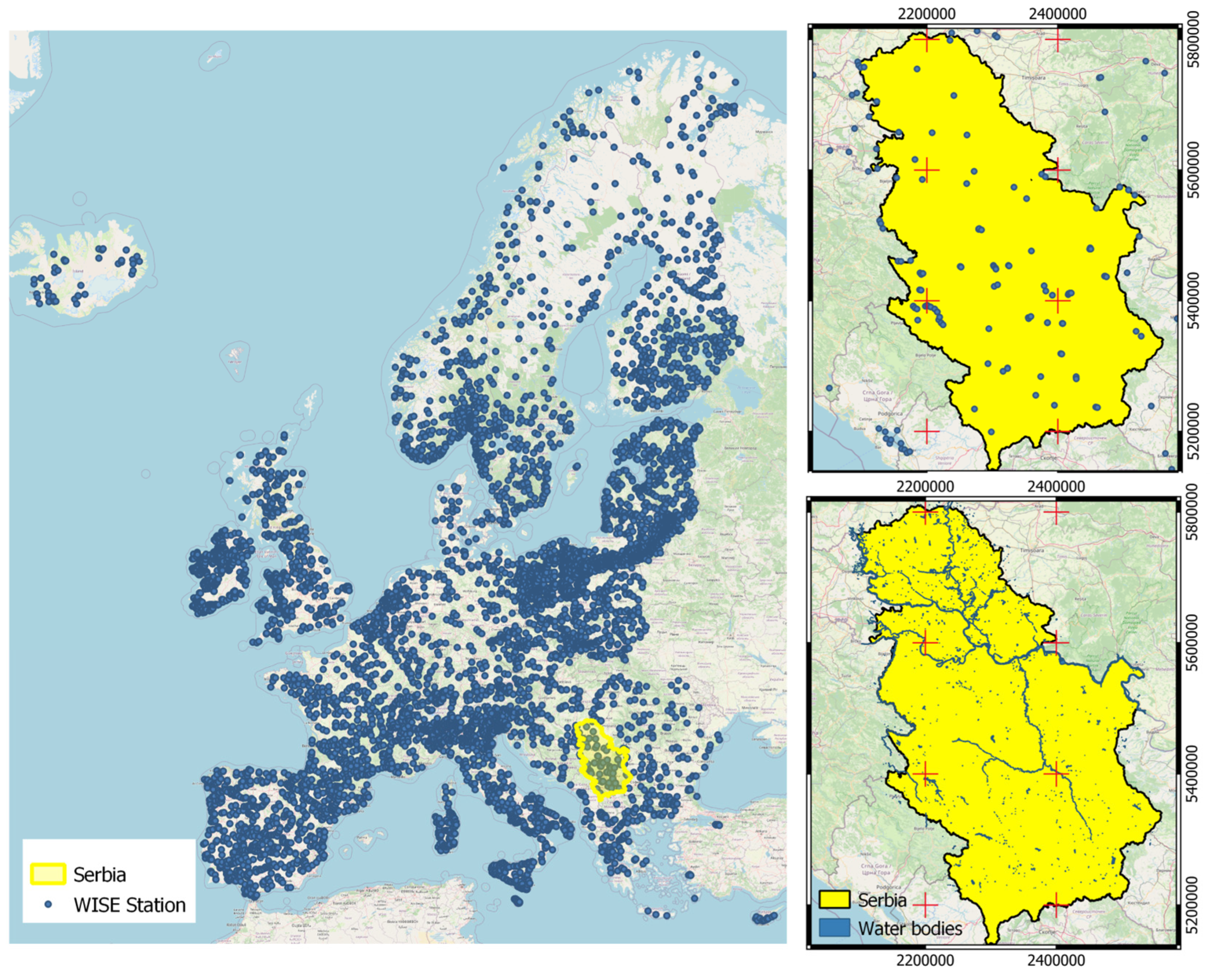
The study area (Figure 1) for this research focused on water quality monitoring based on remote sensing data for the main water bodies within the Republic of Serbia. The Republic of Serbia is located in southeast Europe between 41°53′N and 46°11′N latitude and 18°51′E and 23°01′E longitude. The North part represents the Pannonian Plain with dominant flat terrain while the central and south parts represent hilly regions. Most of the rivers belong to the Black Sea basin. The longest river is the Danube. In addition to the Danube, there are three navigable rivers: Sava, Tisa and part of the Great Morava.
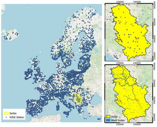
Figure 1.
Study area. (Left): location of the Water Information System of Europe (WISE) monitoring stations in Europe. (Upper Right): Location of monitoring stations in the Republic of Serbia. (Lower Right): Location of main water bodies in Serbia.
On the territory of the Republic of Serbia, there are 498 surface water bodies, 99% of these are represented by streams and 1% are lakes. According to the classification of WFD, these streams are classified as rivers (69%), heavily modified water bodies (28%) and artificial water bodies (3%) [41]. The monitoring program for surface water bodies in the 2017–2019 period includes 137 monitoring stations (123 profiles on streams and 14 locations on accumulations) located on 121 water bodies. In that period, 76% of the water bodies were not included in the monitoring program. The assessment of the ecological potential was performed on 24% of the water bodies from which 2% had a good, 8% moderate, 9% poor, and 5% bad ecological status [42].
2.2. Data
Optical remote sensing monitoring of WQP is based on the correlation between the in-situ measurement and the corresponding surface reflectance.
In this paper, the in-situ data were provided by the Water Information System of Europe (WISE). WISE was launched in 2007, as a joint initiative from European Commission and European Environmental Agency, providing a web portal for water-related information ranging from inland to marine [43]. WISE represents the formal reporting tool for EU water legislation enabling the sharing of water-related information at a European level. The WISE-WFD database contains data reported by EU Member States, Norway and the United Kingdom according to article 13 of the WFD. The database includes aggregated and disaggregated information as well as spatial references about ground and surface water bodies. The disaggregated database represents raw in-situ observed values of WQP [44] reported on an annual basis. Currently, there are more than 60,000,000 in-situ observations and more than 70,000 spatial object identifiers. Data were collected in the period from 1984 to 2022. The sampling location for in-situ water quality monitoring, used in this research, was located along the main inland water bodies (river, lake, and transitional) in Europe to obtain a range of hydrological and atmospheric conditions across a continental scale (Figure 1).
Landsat 5, Landsat 7, and Landsat 8 surface reflectance products from 1984 to 2022 over Europe were used. In total, 213,117 images were analyzed to create a long time series and train the model for WQP monitoring. The date ranges and number of images per sensor are provided in Table 2.
Table 2.
Time frame and number of images per sensor.
Landsat Surface reflectance imagery is atmospherically corrected, containing six (B, G, R, NIR, SWIR, SWIR 2) bands processed to orthorectified surface reflectance using LEDAPS [45]. The Landsat mission is to achieve global coverage once every 16 days with a spatial resolution of 30 m for the multispectral bands. The Google Earth Engine API integrated into Google Colab was used as an access point to the images.
The consistency and standardization of Landsat data across its various missions (Landsat 5, 7 and 8, in this case) is crucial for enabling comparability and consistent analysis over different time periods using time series and to ensure a seamless multi-sensor data record where observed satellite changes can be ascribed to surface changes and not to instrument changes. This consistency is maintained through several factors [46]: (i) rigorous calibration procedures to ensure that sensor characteristics, such as spectral response and radiometric accuracy, remain consistent across the different platforms, to minimize variations between sensors, enabling data continuity [47] (ii) standardized data processing algorithms employed consistently across different Landsat missions, which are corrected for atmospheric effects, geometric distortions, and other artifacts, ensuring that data from different satellites can be combined and compared accurately [48], and (iii) metadata and data format, which documents sensor characteristics, acquisition parameters and processing methods. Although the complete normalization of these factors within the USGS Landsat processing framework remains pending [46], the efforts made to produce consistent and analysis-ready Landsat data across different missions have made possible its broad use for water quality assessment and monitoring [49].
2.3. Methodology
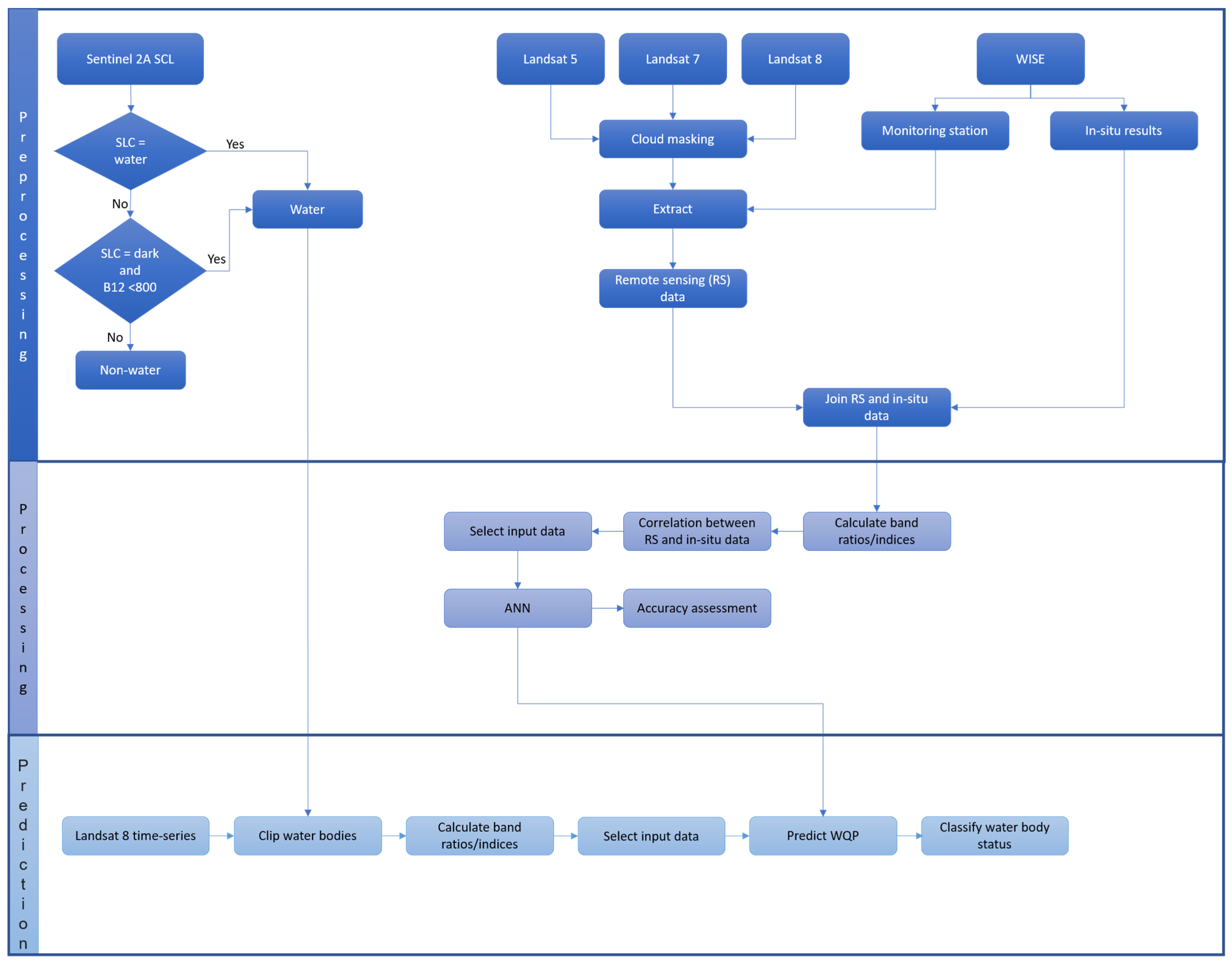
Figure 2 summarizes the approach followed in this paper. It consists of three main steps: preprocessing, processing, and prediction.
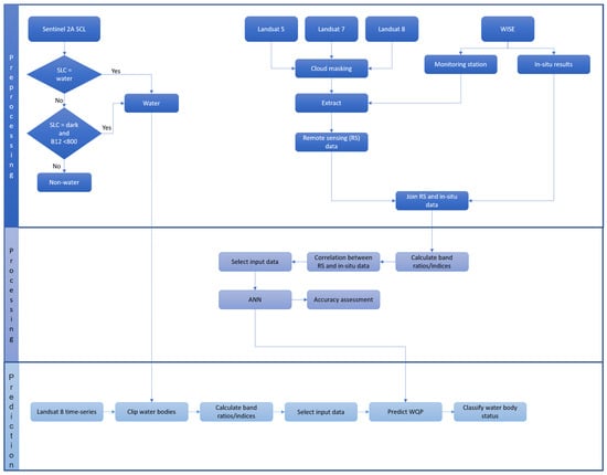
Figure 2.
Workflow.
Preprocessing: The Sentinel 2 Level 2A satellite images were used to detect water bodies. Level 2A was atmospherically corrected by using Sentinel 2 Atmospherically Correction, which is based on [50,51]. The Level 2A images also contain the Scene Classification Layer (SCL), which provides a pixel classification map with four different classes for clouds and six different classes for shadows, cloud shadows, vegetation, soil, water, and snow [52]. Visual inspection showed that water pixels are mostly classified as water or dark pixels. Waterbody masks were created by using the region grow algorithm where water pixels are used as seeds, and neighboring pixels that were classified as dark pixels and had reflectance values lower than 800 in the SWIR 2 band were added to the region. Corresponding water masks were created for each Landsat image used for the prediction of WQP concentration in 2020 in the study area.
The coordinates of the monitoring station were reprojected from WGS84 to WGS84/UTM 34 N projection to match the Landsat imagery coordinate system. Since WQP monitoring is based on remote sensing, the monitoring stations located on small inland water bodies and groundwaters were excluded from the dataset. Additionally, the location of each station was checked against detected water bodies in order to make sure that the extracted value represented water reflectance.
For each point, the values of surface reflectance were extracted from available Landsat 5, Landsat 7, and Landsat 8 Surface Reflectance Level 2A images. The cloud and shadow masking were performed in order to provide clean water pixels. The resulting table contained the identifier of monitoring stations, the corresponding value of surface reflectance, and the sensing date. The surface reflectance was filtered by date to match the in-situ data. The maximum time gap between the in-situ sampling and satellite overpass was 3 days. Final training data contained the surface reflectance of B, G, R, NIR, SWIR1, SWIR 2 band, band ratios NIR/R, G/R, G/B, B/R, R/G, R/B2, NIR/B2, G/SWIR2, spectral indices NDVI, NDWI and NDTU, as well as B*R, G*R, (B + R + NIR)/G and NIR/(R + SWIR) and the corresponding concentration of WQP. The Pearson correlation analysis was used to investigate the association between remote sensing and in-situ data with a correlation coefficient (r). Based on the correlation the input data set for each WQP was defined. The data were standardized to fit a normal distribution with a mean value of 0 and standard deviation of 1 and split into training and test sets (80% and 20%, correspondingly).
Processing: The relationship between the WQP concentration and surface reflectance was modeled by using ANN. ANNs are pattern-recognition algorithms that consist of an interconnected group of artificial neurons, and they process information using a connection approach to computation [53] In this study, a fully connected back-propagation neural network was applied. The network had three layers: input, hidden, and output (Figure 3). The input layer represents predictor or independent variables (in this case radiance measurement of different wavelengths). Hidden layers contain a varying number of neurons. The number of nodes in the hidden layer depends on the complexity of the approximated function and sample numbers. If the network is too small, the self-learning ability and precision of the network will decrease, causing under-fitting. Meanwhile, if the network is too large, training time will increase, and the generalization capability of the network will decrease, producing over-fitting [54]. There is no theoretical formula that can be used for the selection of optimum NN architecture. The architecture was fixed by using a trial-and-error approach. The output values of the hidden layer were the input values of the output layer, which also performs the summation and activation functions. The output of this layer was the target of water quality parameters. To derive the correct output, the network learned by training on the subsets of in-situ data. In the back-propagated network, the outputs were then compared with actual values from the training data set, the error was calculated, and the results were transferred to the output layer. As the data passed through the network many times, weights were adjusted and errors were reduced (Figure 3).
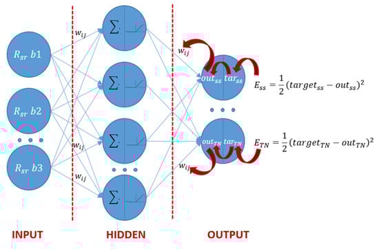
Figure 3.
ANN architecture.
Accuracy assessment: The performance of the developed ANN model was evaluated based on common statistical measures: coefficient of determination (R2) (Equation (1)), RMSE (Equation (2)), normalized RMSE (NRMSE) (Equation (3)), Mean Square Error (MSE) (Equation (4)), Mean Absolute Error (MAE) (Equation (5)). A RMSE measures the quality of the model fit; 0 indicates a perfect fit for the data, while large values are obtained if the estimated concentration of WQP and true concentration differ substantially. NRMSE is used to compare results between models with different scales.
where is actual value, is the predicted value, n sample size, mean of the n actual values, is the maximum of n actual values and is the minimal of n actual values. A model with a high R2 and low RMSE and NRMSE would be suitable for WQP monitoring. The R2 factor is essential for the evaluation of the developed prediction model with the following classification: excellent prediction good prediction , approximate quantitative prediction , a prediction that can possibly distinguish between high and low values , and unsuccessful prediction [55,56].
Prediction: The trained ANN models were used to monitor the WQP concentration based on Landsat 8 Level 2A images for the year 2020 in the study area. Before making the prediction, the images needed to be masked using a water mask (created in the preprocessing phase) in order to ensure that all the pixels represent the water and do not contain surrounding classes. After the prediction of the WQP concentration water quality was classified into classes based on values presented in Table 3. Those values were defined to be in line with those as defined by the legal documents in the field for the Republic of Serbia [57,58,59].
Table 3.
Limit values of WQP concentration for classification of water body status [57,58,59].
In order to gain a deeper insight into the performance of the developed models and assess their practical application, validation was performed. To validate the developed models in the Republic of Serbia, we compared the satellite-derived results and field measurements for the year 2020 for the Zemun monitoring station in the Danube River (which was not included in the training data). Since the in-situ sampling was not regular, there were no matches between the exact dates of satellite-derived results and field sampling, and therefore, the classical statistical measures (R2, RMSE, NRMSE) were not calculated.
2.4. Implementation
The developed workflow was implemented in the Python programming language. The workflow consisted of three modules for the creation of training data, prediction, and monitoring of WQP, and it is fully automated. Manual input is only used for the selection of optimal NN architecture. The remote sensing data were accessed and preprocessed by using GEE Python API. The data set and NN architecture were defined for each WQP. The proposed architecture consisted of input, hidden, and output layers with an activation function (Table 4). The number of the input neurons was selected to be equal to the selected input bands that had a strong correlation with WQPs, and the number of output neurons was selected to be one. The trial-and-error approach was used for the selection of a proper number of hidden neurons. All of the data sets were split at 80% for training and 20% for validation. The learning rate and decay rate were determined through grid search (Learning rate: [0.0001, 0.001, 0.01, 0.1]; Weight decay: [0.000001, 0.00001, 0.0001]). To avoid overfitting, early stopping was used. Early stopping is a commonly used form of regularization that interrupts the training process when there is no improvement of validation loss for a predefined number of epochs. Each time the validation loss improves, the copy of model parameters is stored. After training the algorithm terminates, and those parameters are used instead of the last parameters.
Table 4.
Parameters used to train the model for water quality monitoring.
The training of the networks was conducted using the publicly available cloud platform Collaboratory (Google Colab), which is based on Jupyter Notebooks. The parameters used in the model training are presented in Table 4.
3. Results
The selection of optimal band combination for each WQP was performed (Table 4) allowing for the development of the high-accuracy model. The back-propagated ANN algorithms were proven to be very efficient in monitoring and estimating concentrations of different WQP, for both optically and non-optically active parameters, with highly acceptable results. In general, very positive results were obtained for all WQP and, as shown in Figure 4, coefficients of determination () vary between 0.91 and 0.99 at the validation phase. Since the , the developed models provided an excellent prediction for all WQPs.
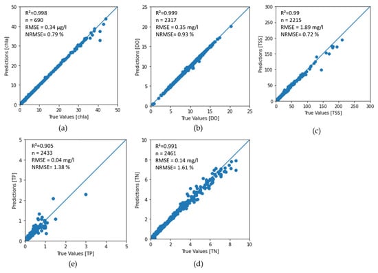
Figure 4.
Graphical fit of predicted results in validation phase (a) chl-a, (b) DO, (c) TSS, (d) TN and (e) TP.
The results of the accuracy assessment are presented in Table 5. As expected, the highest accuracy and lowest NRMSE were obtained for the optically active WQP, i.e., chl-a and TSS (0.79% and 0.72%, respectively).
Table 5.
Accuracy assessment of WQP monitoring using back-propagated ANN algorithms.
The results of the independent validation of the developed model are presented in Table 6, which showed that the models developed for TSS and TN provided accurate classification for all months, while DO reached the lowest values (the water body status matched only in 37.5% of the cases).
Table 6.
Comparison between estimated and measured concentrations of TSS, DO, TN for the Zemun monitoring station in 2020 where M—results of in-situ measurement, P—results of prediction, (C)—water body status based on Table 3. The data for January, February, November and December have been omitted since there were no RS data collected for that period. I–IV are water body status classes.
4. Discussion
4.1. Proposed Model for WQP Monitoring
Aquatic environments have been impacted by various pressures that affect their status and increase water stress. To move towards a more sustainable use of water resources, an appropriate water quality monitoring program needs to be established. In this study, a 38-year long time-series of Landsat and in-situ data were used for the monitoring of WQP based on back-propagated ANN.
As expected, the results of the correlation analysis showed that the highest correlation between remote sensing data and WQP was obtained for TSS. TSS had a significant positive correlation with visible bands and G*R, B*R, and R + NIR while a negative correlation was noticed for G/SWIR. The strong correlation between TSS and visible bands and G*B and B*R was also reported in [20] since higher concentrations of TSS increase water leaving radiance across the whole visible spectrum. Additionally, Refs. [10,60], and others have demonstrated that the R band is suitable for monitoring TSS. Similarly, the highest positive correlation was obtained between chl-a and the green band and the G/B ratio, while the G/SWIR ratio showed a strong negative correlation. The high correlation between chl-a and G bands is consistent with previous studies since water with an increased chl-a concentration reflects a high amount of G radiation [9,61]. DO had a positive correlation with SWIR2, NIR/R and R-NIR while a significant negative correlation was noticed for G/SWIR, R/(B + NIR), and NDWI. The TN and TP had a positive correlation with G, NIR and the R + NIR and NIR band, respectively, while a negative correlation was noticed between TN and NDWI and G/SWIR for TP. The highest correlation between TN and TP and NIR and G band was also reported by [25,62].
According to the results, the highest accuracy (R2, NRMSE [%]) was obtained for chl-a and TSS (Table 5). This is expected since those are optically active water parameters. For chl-a, the accuracy attained in this paper (R2: 0.99, NRMSE: 0.79%) was higher than the ones reported in previous studies. Barraza-Moraga et al. [62] achieved an NRMSE of 3.6% (R2: 0.97, RMSE: 2.58) using Sentinel 2 images to develop an MLE model for chl-a monitoring, while [63] used UAV images and MLR resulting in a R2 of 0.91 and RMSE of 0.07. Along the same lines, Ref. [64] used UAV images to build a CNN model and obtained an R2 of 0.79 (RMSE: 8.76), while [65] used Sentinel 2 images and Ada boost regression resulting in a R2 of 0.90 (RMSE: 1.48). Hafeez et al. [20] used ANN achieving an NRMSE of 5.1% (R2: 0.87, RMSE: 1.4) while [66] reached an R2 of 0.88 using CNN and Sentinel 2 and Geo-Fan 2.
Also, the model developed for monitoring the TSS achieved a high accuracy (R2: 0.99, RMSE: 1.89, NRMSE: 0.72%), larger than the values reported by [65] using Sentinel-2 and RF (R2: 0.6, RMSE: 2.97), and more accurate than the models developed by [20] and [17] using Landsat images and NN, which yielded an R2 of 0.89 (RMSE: 2, NRMSE: 6.2%) and a R2 of 0.93 (RMSE: 0.99, NRMSE: 2.2%), respectively.
Similar results were also obtained for DO, TN and TP (Table 5), with higher accuracies than the ones obtained by [20] to monitor TN using Landsat 8 and a stepwise regression function (R2: 0.61), The same author, when using the RF algorithm, increased the accuracy of R2 to 0.88 [64] and of R2 to 0.94 when using NN [25]. Refs. [22,67] used NN, reaching accuracies of R2 of 0.95 and 0.86, respectively. Lower accuracies were achieved by [22] by using NN to model TN (R2: 0.64, RMSE: 0.04), similar to [56], who used partial least square regression on Landsat 8 and Sentinel 2 data achieving an R2 of 0.63 and 0.77, respectively.
For DO, the accuracies obtained in this study were also higher than the ones obtained by [17,24,68] using NN, or [65], who obtained an R2 of 0.74 by using an Ada boost regression and Sentinel 2 images.
The results in Table 5 showed that NN, as a nonlinear approximation method, provided more accurate results for WQP monitoring. However, the training of NN models requires a large training dataset, otherwise, they may lead to overfitting or underfitting, which greatly limits the extraction of general rules and the generalization ability of the model [69]. Taking into account that most of the previously analyzed papers used small training data sets, such as 125 [22], 60 [25], 155 [64], and 92 [66] samples, it was expected that the proposed method would have a higher accuracy. In addition, the selection of optimal input data as well as the usage of the large time series covering a wide variety of conditions and an early stopping function [70] to avoid overfitting probably had an impact on the increase in the model accuracy.
Regarding the independent validation of the developed model which is shown in (Table 6), although there is no exact coincidence between the date of measurement and estimated concentration, the lowest accuracy was obtained for DO since the water body status matched only in 37.5% of the cases. This can be explained by the high variation of the DO concentration especially in summer months. The results show that the DO concentration can decrease from class I to III within one day [71]. The waterbody status for TP was accurately classified at 75%. However, it was noticed that the developed model tended to overestimate TP during increased concentration. The models developed for TSS and TN provided an accurate classification for all the months. It should be taken into account that the exclusion of monitoring stations located on small inland water bodies and groundwater due to remote sensing-based monitoring limitations might limit the comprehensive coverage of water quality assessments. This exclusion could introduce potential biases in the model’s training dataset, affecting its adaptability to diverse water body sizes and types.
4.2. Usability of the Developed Model in a Real-Case Scenario: Dobrodol Water Reservoir
The developed models and satellite imagery pixel values for larger water bodies in the Republic of Serbia were used to estimate the WQP concentration., since for water management, the classification of water status is necessary. Based on the estimated WQP concentrations and water quality standards for surface water classify each water-quality parameter into five classes indicating water status from “Excellent” to “Bad”.
The change in water body status during 2020 for the Dobrodol water reservoir is presented in Figure 5. It shows that areas close to shorelines with point and diffuse pollution arising from human activity have relatively poor water quality compared to the deeper areas. Generally, the water status of the Dobrodol water body during 2020 could be classified as good, mostly due to the higher concentration of TN. This was expected due to nutrient-rich agriculture discharging from the surrounding land [69]. The visual inspection shows that the chl-a concentration was the highest at the banks and that it decreased when you moved toward the center of the water reservoir, which is in line with either the physical process of sedimentation or algae encroachment [70]. The higher concentration of chl-a was noted during summer. The increase in the growth of algae accelerated the escape of oxygen from the water column, which resulted in an increase of chl-a and a reduction in DO content and the ecological health and balance in the aquatic environment [71,72].
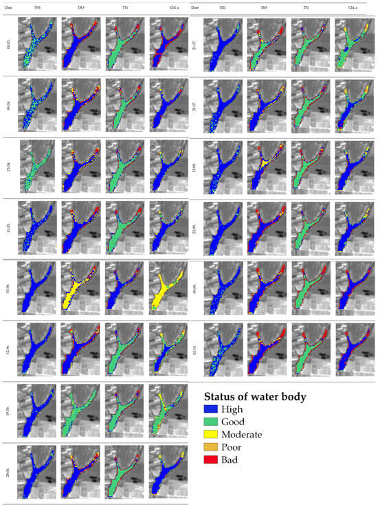
Figure 5.
Water body status classification and spatial variation of WQP for the Dobrodol water body.
5. Conclusions
The study successfully established a robust water quality monitoring program using a 38-year time series of Landsat and in-situ data, coupled with a back-propagated Artificial Neural Network (ANN) model. This model demonstrated high accuracy in monitoring various water quality parameters (WQP), showcasing its potential for sustainable water resource management.
The correlation analysis revealed strong associations between remote sensing data and specific WQPs, such as Total Suspended Solids (TSS), chlorophyll-a (chl-a), Dissolved Oxygen (DO), Total Nitrogen (TN), and Total Phosphorus (TP). Optimal band combinations for each parameter were identified, providing valuable insights into the spectral relationships aiding accurate WQP estimation.
The ANN-based model exhibited exceptional accuracy, particularly for optically active parameters like chl-a and TSS, surpassing results from previous studies that used different remote sensing techniques. This underscores the superiority of the developed model in achieving high precision in WQP estimations, surpassing various existing methods and algorithms.
The study highlighted the efficacy of Neural Networks as a nonlinear approximation method for WQP monitoring. It outperformed other techniques but emphasized the necessity for substantial training datasets to avoid overfitting or underfitting. Optimal input data selection and the use of extensive time series data contributed significantly to model accuracy enhancement.
The independent validation of the developed model revealed a strong ability to classify WQP concentrations accurately. Notably, while the models for TSS and TN provided consistent and accurate classifications, DO estimation faced challenges, especially during high variation periods. This underscores the complexity of DO dynamics in water bodies, particularly during seasonal shifts.
Regarding further research, exploring the integration of additional data sources, such as high-resolution imagery or meteorological data, could further refine the model’s accuracy. Incorporating these data could potentially improve predictions by capturing more intricate environmental parameters that contribute to water quality dynamics. This would contribute to advancing the understanding of the model’s robustness and applicability in different environmental contexts, potentially improving its performance and expanding its utility for broader water quality monitoring and management objectives. Aligning when the sampling data are obtained with satellite overpasses would also be recommended in order to increase the accuracy of the models.
Addressing these weaknesses could potentially strengthen the paper’s findings by providing a more comprehensive assessment of the model’s performance in real scenarios and expanding its applicability across various water body sizes and types.
Author Contributions
Conceptualization, G.J., M.G. and F.Á.-T.; methodology, G.J. and M.G.; software, G.J.; validation, G.J.; formal analysis, G.J., M.G. and F.Á.-T.; investigation, G.J.; writing—original draft preparation, G.J. and M.G.; writing—review and editing, G.J., M.G. and F.Á.-T.; visualization, G.J.; supervision M.G. and F.Á.-T. All authors have read and agreed to the published version of the manuscript.
Funding
This research received no external funding.
Data Availability Statement
The used data are available at https://github.com/jakovljevicg/WQP (accessed on 20 December 2023).
Acknowledgments
The authors would like to thank the anonymous reviewers who helped improve the manuscript with their comments and suggestions.
Conflicts of Interest
The authors declare no conflict of interest.
References
- UN General Assembly. Transforming Our World: The 2030 Agenda for Sustainable Development. 21 October 2015. Available online: https://www.refworld.org/docid/57b6e3e44.html (accessed on 5 December 2022).
- United Nations. Goal 6: Ensure Access to Water and Sanitation for All; UN: New York, NY, USA, 2018. [Google Scholar]
- European Parliament. Directive 2000/60/EC—Framework for Community Action in the Field of Water Policy; European Parliament: Bruxelles, Belgium, 2003. [Google Scholar]
- European Communities. Guidance Document n.o 7 Monitoring under the Water Framework Directive; Office for Official Publica-tions of the European Communities: Luxembourg, 2003. [Google Scholar]
- He, J.; Chen, Y.; Wu, J.; Stow, D.A.; Christakos, G. Space-Time Chlorophyll-a Retrieval in Optically Complex Waters that Accounts for Remote Sensing and Modeling Uncertainties and Improves Remote Estimation Accuracy. Water Res. 2019, 171, 115403. [Google Scholar] [CrossRef]
- Nas, B.; Ekercin, S.; Karabörk, H.; Berktay, A.; Mulla, D.J. An Application of Landsat-5TM Image Data for Water Quality Mapping in Lake Beysehir, Turkey. Water Air Soil Pollut. 2010, 212, 183–197. [Google Scholar] [CrossRef]
- Govedarica, M.; Jakovljevic, G. Monitoring spatial and temporal variation of water quality parameters using time series of open multispectral data. In Proceedings of the SPIE 11174 Seventh International Conference on Remote Sensing and Geoinformation of the Environment, Paphos, Cyprus, 18–21 March 2019. [Google Scholar]
- Wu, C.; Wu, J.; Qi, J.; Zhang, L.; Huang, H.; Lou, L.; Chen, Y. Empirical estimation of total phosphorus concentration in the mainstream of the Qiantang River in China using Landsat TM data. Int. J. Remote Sens. 2010, 31, 2309–2324. [Google Scholar] [CrossRef]
- Ha, N.; Koike, K.; Nhuan, M. Improved Accuracy of Chlorophyll-a Concentration Estimates from MODIS Imagery Using a Two-Band Ratio Algorithm and Geostatistics: As Applied to the Monitoring of Eutrophication Processes over Tien Yen Bay (Norther Vietnam). Remote Sens. 2013, 6, 421–442. [Google Scholar] [CrossRef]
- Nechad, B.; Ruddick, K.; Park, Y. Calibration and validation of a generic multisensor algorithm for mapping of total suspended matter in turbid waters. Remote Sens. Environ. 2010, 114, 854–866. [Google Scholar] [CrossRef]
- Zhang, Y.; Wu, Z.; Liu, M.; He, J.; Shi, K.; Wang, M.; Yu, Z. Thermal structure and response to long-term climatic changes in Lake Qiandaohu, a deep subtropical reservoir in China. Limnol. Oceanogr. 2014, 59, 1193–1202. [Google Scholar] [CrossRef]
- Brezonik, P.L.; Olmanson, L.G.; Finlay, J.C.; Bauer, M.E. Factors Affecting the Measurement of CDOM by Remote Sensing of Optically Complex Inland Waters. Remote Sens. Environ. 2015, 157, 199–215. [Google Scholar] [CrossRef]
- Shahzad, M.I.; Meraj, M.; Nazeer, M.; Zia, I.; Inam, A.; Mehmood, K.; Zafar, H. Empirical Estimation of Suspended Solids Concentration in the Indus Delta Region Using Landsat-7 ETM+ Imagery. J. Environ. Manag. 2018, 209, 254–261. [Google Scholar] [CrossRef]
- Bonansea, M.; Rodriguez, M.C.; Pinotti, L.; Ferrero, S. Using multitemporal Landsat imagery and linear mixed models for assessing water quality parameters in Río Tercero reservoir (Argentina). Remote Sens. Environ. 2015, 158, 28–41. [Google Scholar] [CrossRef]
- Lim, J.; Choi, M. Assessment of water quality based on Landsat 8 operational land imager associated with human activities in Korea. Environ. Monit. Assess. 2015, 187, 1–7. [Google Scholar] [CrossRef]
- Ekercin, S. Water Quality Retrievals from High Resolution Ikonos Multispectral Imagery: A Case Study in Istanbul, Turkey. Water Air Soil Pollut. 2007, 183, 239–251. [Google Scholar] [CrossRef]
- Din, E.S.E.; Zhang, Y.; Suliman, A. Mapping concentrations of surface water quality parameters using a novel remote sensing and artificial intelligence framework. Int. J. Remote Sens. 2017, 38, 1023–1042. [Google Scholar] [CrossRef]
- Umar, M.; Rhoads, B.L.; Greenberg, J.A. Use of multispectral satellite remote sensing to assess mixing of suspended sediment downstream of large river confluences. J. Hydrol. 2018, 556, 325–338. [Google Scholar] [CrossRef]
- Guo, Y.; Deng, R.; Li, J.; Hua, Z.; Wang, J.; Zhang, R.; Liang, Y.; Tang, Y. Remote Sensing Retrieval of Total Nitrogen in the Pearl River Delta Based on Landsat8. Water 2022, 14, 3710. [Google Scholar] [CrossRef]
- Hafeez, S.; Wong, M.S.; Ho, H.C.; Nazeer, M.; Nichol, J.E.; Abbas, S.; Tang, D.; Lee, K.-H.; Pun, L. Comparison of Machine Learning Algorithms for Retrieval of Water Quality Indicators in Case-II Waters: A Case Study of Hong Kong. Remote Sens. 2019, 11, 617. [Google Scholar] [CrossRef]
- Li, Y.; Zhang, Y.; Shi, K.; Zhu, G.; Zhuo, Y.; Zhang, Y.; Guo, Y. Monitoring spatiotemporal variations in nutrients in a large drinking water reservoir and their relationships with hydrological and meteorological conditions based on Landsat 8 imagery. Sci. Total. Environ. 2017, 599, 1705–1717. [Google Scholar] [CrossRef]
- Vakili, T.; Amanollahi, J. Determination of optically inactive water quality variables using Landsat 8 data: A case study in Geshlagh reservoir affected by agricultural land use. J. Clean. Prod. 2019, 247, 119134. [Google Scholar] [CrossRef]
- Guo, H.; Huang, J.J.; Zhu, X.; Wang, B.; Tian, S.; Xu, W.; Mai, Y. A generalized machine learning approach for dissolved oxygen estimation at multiple spatiotemporal scales using remote sensing. Environ. Pollut. 2021, 288, 117734. [Google Scholar] [CrossRef] [PubMed]
- Qian, J.; Liu, H.; Qian, L.; Bauer, J.; Xue, X.; Yu, G.; He, Q.; Zhou, Q.; Bi, Y.; Norra, S. Water quality monitoring and assessment based on cruise monitoring, remote sensing, and deep learning: A case study of Qingcaosha Reservoir. Front. Environ. Sci. 2022, 10, 979133. [Google Scholar] [CrossRef]
- Guo, H.; Huang, J.J.; Chen, B.; Guo, X.; Singh, V.P. A machine learning-based strategy for estimating non-optically active water quality parameters using Sentinel-2 imagery. Int. J. Remote Sens. 2020, 42, 1841–1866. [Google Scholar] [CrossRef]
- Peterson, K.T.; Sagan, V.; Sloan, J.J. Deep learning-based water quality estimation and anomaly detection using Land-sat-8/Sentinel-2 virtual constellation and cloud computing. Giscience Remote Sens. 2020, 57, 510–525. [Google Scholar] [CrossRef]
- Leggesse, E.S.; Zimale, F.A.; Sultan, D.; Enku, T.; Srinivasan, R.; Tilahun, S.A. Predicting Optical Water Quality Indicators from Remote Sensing Using Machine Learning Algorithms in Tropical Highlands of Ethiopia. Hydrology 2023, 10, 110. [Google Scholar] [CrossRef]
- Gómez, D.; Salvador, P.; Sanz, J.; Casanova, J.L. A new approach to monitor water quality in the Menor sea (Spain) using satellite data and machine learning methods. Environ. Pollut. 2021, 286, 117489. [Google Scholar] [CrossRef] [PubMed]
- Balabin, R.M.; Lomakina, E.I. Support vector machine regression (SVR/LS-SVM)—An alternative to neural networks (ANN) for analytical chemistry? Comparison of nonlinear methods on near infrared (NIR) spectroscopy data. Analyst 2011, 136, 1703–1710. [Google Scholar] [CrossRef] [PubMed]
- Jakovljevic, G.; Govedarica, M.; Alvarez-Taboada, F. Water body mapping: A comparison of remotely sensed and GIS open data sources. Int. J. Remote Sens. 2018, 40, 2936–2964. [Google Scholar] [CrossRef]
- Nolan, B.T.; Fienen, M.N.; Lorenz, D.L. A statistical learning framework for groundwater nitrate models of the Central Valley, California, USA. J. Hydrol. 2015, 531, 902–911. [Google Scholar] [CrossRef]
- Singh, K.P.; Basant, N.; Gupta, S. Support vector machines in water quality management. Anal. Chim. Acta 2011, 703, 152–162. [Google Scholar] [CrossRef] [PubMed]
- Liu, M.; Lu, J. Support vector machine―An alternative to artificial neuron network for water quality forecasting in an agricultural nonpoint source polluted river? Environ. Sci. Pollut. Res. 2014, 21, 11036–11053. [Google Scholar] [CrossRef]
- Kim, Y.H.; Im, J.; Ha, H.K.; Choi, J.-K.; Ha, S. Machine learning approaches to coastal water quality monitoring using GOCI satellite data. GIScience Remote Sens. 2014, 51, 158–174. [Google Scholar] [CrossRef]
- Li, M.; Im, J.; Beier, C. Machine learning approaches for forest classification and change analysis using multitemporal Landsat TM images over Huntington Wildlife Forest. GIScience Remote Sens. 2013, 50, 361–384. [Google Scholar] [CrossRef]
- Ramezan, C.A.; Warner, T.A.; Maxwell, A.E.; Price, B.S. Effects of Training Set Size on Supervised Machine-Learning Land-Cover Classification of Large-Area High-Resolution Remotely Sensed Data. Remote Sens. 2021, 13, 368. [Google Scholar] [CrossRef]
- Zeng, W.; Xu, K.; Cheng, S.; Zhao, L.; Yang, K. Regional Remote Sensing od Lake Water Transparency Based on Google Earth Engine: Preformance of Empircal Algorithm and Machine Learning. Appl. Sci. 2023, 13, 4007. [Google Scholar] [CrossRef]
- Pu, F.; Ding, C.; Chao, Z.; Yu, Y.; Xu, X. Water-Quality Classification of Inland Lakes Using Landsat8 Images by Convolutional Neural Networks. Remote Sens. 2019, 11, 1674. [Google Scholar] [CrossRef]
- Cui, Y.; Yan, Z.; Wang, J.; Hao, S.; Liu, Y. Deep learning–based remote sensing estimation of water transparency in shallow lakes by combining Landsat 8 and Sentinel 2 images. Environ. Sci. Pollut. Res. 2021, 29, 4401–4413. [Google Scholar] [CrossRef] [PubMed]
- Aptoula, E.; Ariman, S. Chlorophyll-a Retrieval from Sentinel-2 Images Using Convolutional Neural Network Regression. IEEE Geosci. Remote Sens. Lett. 2021, 19, 1–5. [Google Scholar] [CrossRef]
- Sl Glasnik RS br 96/2010. Pravilnik o Utvrđivanju Vodnih tela Površinskih i Podzemnih Voda; Sl glasnik RS: Beograd, Serbia, 2010. [Google Scholar]
- Agencija za zastitu zivotne sredine. Ministarstvo za Zaštitu Životne Sredine Status Površinskih voda Srbije u Periodu od 2017–2019; Agencija za zastitu zivotne sredine: Beograd, Serbia, 2021. [Google Scholar]
- European Environment Agency. WISE. Available online: https://water.europa.eu/#:~:text=The%20Water%20Information%20System%20for,from%20inland%20waters%20to%20marine (accessed on 1 December 2022).
- European Environment Agency. Eionet. Available online: https://dd.eionet.europa.eu/tables/11122 (accessed on 1 December 2022).
- USGS. Landsat 4-7 Collection 1 Surface Reflectance Code LEDAPS Product Guide. Available online: https://d9-wret.s3.us-west-2.amazonaws.com/assets/palladium/production/s3fs-public/atoms/files/LSDS-1370_L4-7_C1-SurfaceReflectance-LEDAPS_ProductGuide-v3.pdf (accessed on 25 November 2022).
- Wulder, M.A.; Roy, D.P.; Radeloff, V.C.; Loveland, T.R.; Anderson, M.C.; Johnson, D.M.; Healey, S.; Zhu, Z.; Scambos, T.A.; Pahlevan, N.; et al. Fifty years of Landsat science and impacts. Remote Sens. Environ. 2022, 280. [Google Scholar] [CrossRef]
- Mishra, N.; Haque, M.O.; Leigh, L.; Aaron, D.; Helder, D.; Markham, B. Radiometric Cross Calibration of Landsat 8 Operational Land Imager (OLI) and Landsat 7 Enhanced Thematic Mapper Plus (ETM+). Remote Sens. 2014, 6, 12619–12638. [Google Scholar] [CrossRef]
- Mishra, N.; Helder, D.; Barsi, J.; Markham, B. Continuous calibration improvement in solar reflective bands: Landsat 5 through Landsat 8. Remote Sens. Environ. 2016, 185, 7–15. [Google Scholar] [CrossRef]
- Yang, H.; Kong, J.; Hu, H.; Du, Y.; Gao, M.; Chen, F. A Review of Remote Sensing for Water Quality Retrieval: Progress and Challenges. Remote Sens. 2022, 14, 1770. [Google Scholar] [CrossRef]
- Richter, R.; Schläpfer, D. Atmospheric/Topographic Correction for Satellite Imagery: ATCOR-2/3 UserGuide; DLR: Wessling, Germany, 2011. [Google Scholar]
- Mayer, B.; Kylling, A. Technical note: The libRadtran software package for radiative transfer calculations—description and examples of use. Atmos. Chem. Phys. 2005, 5, 1855–1877. [Google Scholar] [CrossRef]
- ESA. Level-2A Algorithm Overview. Available online: https://earth.esa.int/web/sentinel/technical-guides/sentinel-2-msi/level-2a/algorithm (accessed on 15 August 2020).
- Fausset, L.V. Fundamentals of Neural Networks: Architectures, Algorithms and Applications; Pearson: New York, NY, USA, 1993. [Google Scholar]
- Krasnopolsky, V.; Gemmill, W.; Breaker, L. A neural network multipara meter algorithm for SSM/I ocean retrievals: Comparisons and validations. Remote Sens. Environ. 2000, 72, 133–142. [Google Scholar] [CrossRef]
- Vohland, M.; Besold, J.; Hill, J.; Fründ, H.-C. Comparing different multivariate calibration methods for the determination of soil organic carbon pools with visible to near infrared spectroscopy. Geoderma 2011, 166, 198–205. [Google Scholar] [CrossRef]
- Liang, Y.; Yin, F.; Xie, D.; Liu, L.; Zhang, Y.; Ashraf, T. Inversion and Monitoring of the TP Concentration in Taihu Lake Using the Landsat-8 and Sentinel-2 Images. Remote Sens. 2022, 14, 6284. [Google Scholar] [CrossRef]
- S. R. b. 74/2011. Uredba o klasifikaciji Voda; Sluzbeni glasnik RS: Beograd, Serbia, 1968. [Google Scholar]
- S. R. b. 50/2012. Uredba o Graničnim Vrednostima Zagađujućih Materija u Površinskim i Podzemnim Vodama i Sedimentu i Rokovima za Njihovo Dostizanje; Sluzbeni Glasnik: Beograd, Serbia, 2012. [Google Scholar]
- S. R. b. 74/2011. Pravilnik o Parametrima Ekološkog i Hemijskog Statusa Površinskih Voda i Parametrima Hemijskog i Kvantitativnog Statusa Podzemnih Voda; Sluzbeni Glasnik: Beograd, Serbia, 2011. [Google Scholar]
- Miller, R.L.; McKeen, B.A. Using MODIS Terra 250 m Imagery to Map Concentrations of Total Suspended Matter in Coastal Waters. Remote Sens. Environ. 2004, 93, 259–266. [Google Scholar] [CrossRef]
- Sadeghi, A.; Dinter, T.; Vountas, M.; Taylor, B.B.; Altenburg-Soppa, M.; Peeken, I.; Bracher, A. Improvement to the PhytoDOAS method for identification of coccolithophores using hyperspectral satellite data. Ocean Sci. 2012, 8, 1055–1070. [Google Scholar] [CrossRef]
- Barraza-Moraga, F.; Alcayaga, H.; Pizarro, A.; Félez-Bernal, J.; Urrutia, R. Estimation of Chlorophyll-a Concentrations in Lanalhue Lake Using Sentinel-2 MSI Satellite Images. Remote Sens. 2022, 14, 5647. [Google Scholar] [CrossRef]
- Roman, A.; Tovar-Sanchez, A.; Gauci, A.; Deidun, A.; Cabellero, I.; Colica, E.; D’Amivo, S.; Navarro, G. Water-Quality Moni-toring with a UAV-Mounted Multispectral Camera in Coastal Waters. Remote Sens. 2023, 15, 237. [Google Scholar] [CrossRef]
- Zhao, X.; Li, Y.; Chen, Y.; Qiao, X.; Qian, W. Water Chlorophyll a Estimation Using UAV-Based Multispectral Data and Machine Learning. Drones 2023, 7, 2. [Google Scholar] [CrossRef]
- Quang, N.H.; Dinh, N.T.; Dien, N.R.; Son, L.T. Calibration of Sentinel-2 Surface Reflectance for Water Quality Modelling in Binh Dinh’s Coastal Zone of Vietnam. Sustainability 2023, 15, 1410. [Google Scholar] [CrossRef]
- Yang, H.; Du, Y.; Zhao, H.; Chen, F. Water Quality Chl-a Inversion Based on Spatio-Temporal Fusion and Convolutional Neural Network. Remote Sens. 2022, 14, 1267. [Google Scholar] [CrossRef]
- Chebud, Y.A.; Naja, G.M.; Rivero, R.G.; Melessa, A.M. Water Quality Monitoring Using Remote Sensing and an Artificial Neural Network. Water Air Soil Pollut. 2012, 223, 4875–4887. [Google Scholar] [CrossRef]
- Ahmed, M.; Mumtaz, R.; Anwar, Z.; Shaukat, A.; Arif, O.; Shafait, F. A Multi–Step Approach for Optically Active and Inactive Water Quality Parameter Estimation Using Deep Learning and Remote Sensing. Water 2022, 14, 2112. [Google Scholar] [CrossRef]
- Schmidhuber, J. Deep Learning in Neural Networks: An Overview. arXiv 2014, arXiv:1404.7828v4. [Google Scholar] [CrossRef] [PubMed]
- Prechelt, L. Early Stopping—But When. In Neural Networks: Tricks of the Trade; Springer: Berlin, Germany, 2012; pp. 53–67. [Google Scholar]
- SEPA. Stanje Kvaliteta Vode Vodotoka. Agencija za Životnu Sredinu. Available online: http://77.46.150.213:8080/apex/f?p=406:2:::::: (accessed on 15 October 2023).
- Seyhan, E.; Dekker, A. Application of remote sensing techniques for water quality monitoring. Aquat. Ecol. 1986, 20, 41–50. [Google Scholar] [CrossRef]


Disclaimer/Publisher’s Note: The statements, opinions and data contained in all publications are solely those of the individual author(s) and contributor(s) and not of MDPI and/or the editor(s). MDPI and/or the editor(s) disclaim responsibility for any injury to people or property resulting from any ideas, methods, instructions or products referred to in the content. |
© 2023 by the authors. Licensee MDPI, Basel, Switzerland. This article is an open access article distributed under the terms and conditions of the Creative Commons Attribution (CC BY) license (https://creativecommons.org/licenses/by/4.0/).