Abstract
In recent years, the use of deep neural network in effective network feature extraction and the design of efficient and high-precision hyperspectral image classification algorithms has gradually become a research hotspot for scholars. However, due to the difficulty of obtaining hyperspectral images and the high cost of annotation, the training samples are very limited. In order to cope with the small sample problem, researchers often deepen the network model and use the attention mechanism to extract features; however, as the network model continues to deepen, the gradient disappears, the feature extraction ability is insufficient, and the computational cost is high. Therefore, how to make full use of the spectral and spatial information in limited samples has gradually become a difficult problem. In order to cope with such problems, this paper proposes two-branch multiscale spatial–spectral feature aggregation with a self-attention mechanism for a hyperspectral image classification model (FHDANet); the model constructs a dense two-branch pyramid structure, which can achieve the high efficiency extraction of joint spatial–spectral feature information and spectral feature information, reduce feature loss to a large extent, and strengthen the model’s ability to extract contextual information. A channel–space attention module, ECBAM, is proposed, which greatly improves the extraction ability of the model for salient features, and a spatial information extraction module based on the deep feature fusion strategy HLDFF is proposed, which fully strengthens feature reusability and mitigates the feature loss problem brought about by the deepening of the model. Compared with five hyperspectral image classification algorithms, SVM, SSRN, A2S2K-ResNet, HyBridSN, SSDGL, RSSGL and LANet, this method significantly improves the classification performance on four representative datasets. Experiments have demonstrated that FHDANet can better extract and utilise the spatial and spectral information in hyperspectral images with excellent classification performance under small sample conditions.
1. Introduction
Hyperspectral remote sensing is a multidimensional information acquisition technology that integrates imaging technology and spectral technology, simultaneously detecting two-dimensional spatial information and one-dimensional spectral information of the feature target, so as to obtain hyperspectral images (HSIs) with high spectral resolution and many bands. HSIs can reflect nearly continuous spectral characteristic curves of the feature, containing rich spatial and spectral information, and is a comprehensive carrier of various information. The use of hyperspectral data spectral unity and the characteristics of a wide range of band coverage can greatly improve its ability to distinguish the identification of feature classes [1]; thus, hyperspectral remote sensing technology has been widely applied to the refinement of agriculture [2,3], military applications [4,5], environmental monitoring [6,7] and other aspects.
Hyperspectral image classification (HIC) is the foundation of various hyperspectral applications. The main goal of HIC is to adjudicate the pixels in an image so as to achieve the automatic identification of feature classes for other sectors. From classical machine learning theories, such as SVM [8] and KNN [9], to deep neural networks (DNNs), deep learning model frameworks represented by convolutional neural networks have been widely used for HIC and have achieved remarkable success. Before 2012, deep learning algorithms based on neural networks had not been popularized due to the large scale of computing parameters and insufficient hardware to support such large-scale parameter operations. However, 2012 was an epochal year in which AlexNet [10] made a major breakthrough in the ImageNet competition held by Google, and deep learning algorithms based on convolutional neural networks (CNNs)-based deep learning algorithms began to be emphasized, and deep learning algorithms about CNNs, such as VGG (16/19) [10], ResNet [11], etc., have been continuously proposed and applied to the fields of image categorization, target detection, and image style conversion. With the continuous development of CNNs, HIC algorithms based on convolutional neural networks have gradually become one of the research hotspots. Hu et al. [12] proposed a five-layer convolutional neural network for hyperspectral image classification and achieved good classification results. Yue et al. [13] introduced the spatial and spectral information in the hyperspectral image into the CNN model after fusion, which further improved the classification effect. Zhao et al. [14] extracted the spectral and spatial relationship information of neighboring pixel pairs by using the twin neural network and utilized the Softmax loss function to achieve classification. Wu et al. [15] used 1D-CNN and 2D-CNN to extract spectral and spatial features, respectively; however, when using 1D-CNN for spectral feature learning, a large number of convolution kernels are required in the face of the high number of bands in HSI, which results in excessive computation and likely overfitting. To alleviate this problem, Chen et al. [16] made the first attempt to use training sample chunks to train CNNs for deep feature extraction and the classification of HSIs. Thanks to the powerful automatic feature extraction capability of CNNs, many deep CNN models based on training sample chunks for extracting spectral–patial joint features have been proposed [17,18,19,20]. Roy et al. [21] proposed HybridSN networks based on 3D-CNN and 2D-CNN, where 3D-CNN is used to extract spectral–stereo spatial information, and 2D-CNN is further used to extract the planar spatial information. However, HybridSN does not fully consider the rich spectral and spatial information of HSI itself, and there is still room for improvement in the extraction and utilization of spatial and spectral information of HSIs. Zhang et al. [22] proposed a differential region convolutional neural network (DRCNN)-based approach that uses different image blocks within the neighborhood of the target pixel as the input to the CNN, where the input data are effectively reinforced. Roy et al. [23] used attention-based adaptive spectral–spatial kernel residual network (A2S2K-ResNet) to mine more discriminative joint spectral–spatial features. Pu et al. [24] used convolutional kernel-adaptive rotation to extract features in different orientations of an object. Yang et al. [25] proposed a supervised change detection method based on deep concatenated semantic segmentation network to process the data efficiently. Scheibenreif et al. [26] used self-supervised mask image reconstruction to advance the transformer model for hyperspectral remote sensing images.
Due to the special data characteristics of HSIs, there are still several challenges in building network models using convolutional neural networks [27,28]: (1) The spectral dimension of HSI has hundreds of band values, and the information between bands has redundancy, resulting in high data dimensionality and, therefore, rich spectral information. However, when the number of available labeled samples is limited, this high dimensionality characteristic of the data will introduce the curse of dimensionality problem (usually also becomes Hughes phenomenon), i.e., with the increase in the number of bands involved in the operation, the classification accuracy increases and then decreases. (2) The high cost of HSI sample labeling leads to insufficient labeled samples, which lead to the model overfitting phenomenon, resulting in low generalization performance. (3) Due to the role of convolutional kernel and pooling layer, as the network continues to deepen, it will cause unavoidable feature loss, insufficient feature extraction, and other problems.
Based on the above problems, researchers must consider both the rich spectral and spatial information extraction of HSI when designing network models. However, pure 3D-CNN is not widely used due to its huge computational volume. The computational resources consumed are huge; therefore, pure 3D-CNN is not widely used. Moreover, pure 2D-CNN is not widely used in the field of HIC due to its inability to deal with spectral dimensional data information; in other words, pure 2D-CNN restricts itself to spatial information features, and thus, pure 2D-CNN cannot shine in the field of HIC. To sum up, researchers considered combining 2D-CNN and 3D-CNN and used 3D-CNN’s powerful computational ability as a spectral spatial information feature extractor and 2D-CNN as a pure spatial feature extractor. From this, the 3D-2D-CNN structure came into being. Roy constructed a classification model for hyperspectral images using 3D-2D-CNN in HyBridSN, but he ignored the fact that the 3D-2D-CNN structure was not a good choice for classification. Roy used 3D-2D-CNN structure in HyBridSN to complete the construction of hyperspectral image classification models, but he neglected one point, that is, the continuous stacking of convolutional blocks will inevitably lead to the loss of feature information, which is an inherent defect of the convolutional computation and so can not be avoided. In addition, the model’s ability to extract salient features is insufficient, which leads to the unsatisfactory performance of the model in small samples. Feng et al. [29]. proposed R-HyBridSN, which is based on HyBridSN, and uses the so-called depth-separable convolution and residual convolution blocks to optimize HyBridSN to a certain extent but the model’s ability to extract salient features of HSI is still insufficient. The saliency feature extraction abilities are still insufficient, and the large number of 3D-CNN leads to the significant consumption of computational resources by the model. However, from another point of view, we cannot deny that the 3D-2D-CNN architecture is more advantageous for HIC. Zhang et al. [30] proposed a DPCMF model that has a dense pyramid connection structure with a two-branch structure, which effectively alleviates the performance degradation caused by the feature loss, but the DPCMF uses the 3D convolutional block as the model. However, DPCMF uses 3D convolutional blocks as the base component of the model, which leads to a very large number of computational resources being consumed by the model. Secondly, HSI data contain very complex spectral and spatial information, and the simple two-branch structure of DPCMF directly fuses the high-level feature maps generated by the two branches and then classifies them, which leads to the lack of extraction of complex features for HSI; however, there are not enough parameters to fit the complex data distributions, and the results obtained are not satisfactory. However, it is undeniable that the two-branch structure has a unique advantage for the HIC task; that is, each branch of the two-branch structure can use different network structures and parameters to capture the spatial and spectral features of the input HSI data.
How can the advantages of the 3D-2D-CNN architecture be better exploited under small sample conditions? How can we effectively mitigate the problem of insufficient model feature extraction capabilities and feature loss caused by deepening network hierarchy? Generally speaking, as the network continues to deepen, the extracted features will gradually transform form low-level features to high-level features; however, under the objective conditions of the CNN limitations, it will cause a certain degree of feature loss, and also lead to model training difficulties, gradient disappearance, and other problems. The traditional residual connection and dense connection can alleviate the above problems but the effect is always unsatisfactory; the reason is that the model in the process of training is not the same attention to the attention to the features. In order to solve this problem, the attention mechanism has gradually become a hotspot for the application of HIC, ref. [31] proposed a dense CNN network based on feedback attention, and ref. [32] proposed a convolutional block-based attention module (CBAM) [33] for a dual-branch multiple attention mechanism network (DBMA). Although these methods have better results, they are not targeted to solve the problems of feature loss and insufficient feature extraction, especially in the case of limited samples, the feature loss has a very large impact on the HIC effect, and could not obtain satisfactory classification results.
Aiming at the problems of missing features and insufficient ability to extract features in the feature extraction process of CNN models, we propose a high-precision HIC model with two-branch multiscale feature aggregation and multiple attention mechanisms inspired by the two-branch structure and attention mechanisms. The model extracts multiscale spatial–spectral feature information using a joint spatial–spectral branch and a spectral branch, respectively. The original HSI processing dimensionality reduction is performed using FA (factor analysis), where significant spectral information is preserved, while the rest of the redundant information and noise are removed. In the two-branch dense connection mechanism, each branch consists of different convolutional blocks that are densely connected to form a dense pyramid connection. In the joint spatial–spectral feature extraction process, the dense pyramid convolution is used to extract the multiscale spatial–spectral feature information in the sample; in the spectral branch, the dense pyramid convolution layer is used to extract the spectral features. Subsequently, the two-branch feature maps are fused and fed to the spatial feature extractor. During the construction of the spatial feature extractor, we propose a new efficient channel–spatial block attention nodule (ECBAM) to enhance the model’s ability to extract salient features; we propose a deep feature fusion strategy high–low deep feature fusion strategy (HLDFF), specifically to enhance the spatial feature learning ability via inverse convolution. Finally, the obtained feature maps are input into the classifier to obtain the classification results. The three main contributions of this paper are as follows:
- (1)
- In order to alleviate the problem of insufficient feature missing, a two-branch multiscale feature aggregation with multiple attention mechanism is proposed as a HIC model, which extracts multiscale joint spatial–spectral feature information fusion to obtain hyperspectral feature maps by using dense pyramidal joint spatial–spectral feature extraction branches and inter-spectral feature extraction branches, respectively.
- (2)
- In order to enhance the level of attention to significant features during spatial feature extraction, an efficient channel–spatial block attention module (ECBAM) is proposed to enhance the expressiveness of salient spatial information.
- (3)
- In the process of spatial feature extraction, a high–low deep feature fusion strategy (HLDFF) is proposed to implement up-sampling of the high-level feature maps and cleverly fuse them with the low-level feature maps to obtain richer feature representations.
The rest of the paper is organized as follows: Section 2 presents the concrete implementation of the proposed model. Section 3 presents and analyses the experimental results, Section 4 discusses the experimental results. Section 5 summarizes the conclusions of the paper and gives directions for future research.
2. Materials and Methods
2.1. Overall Framework
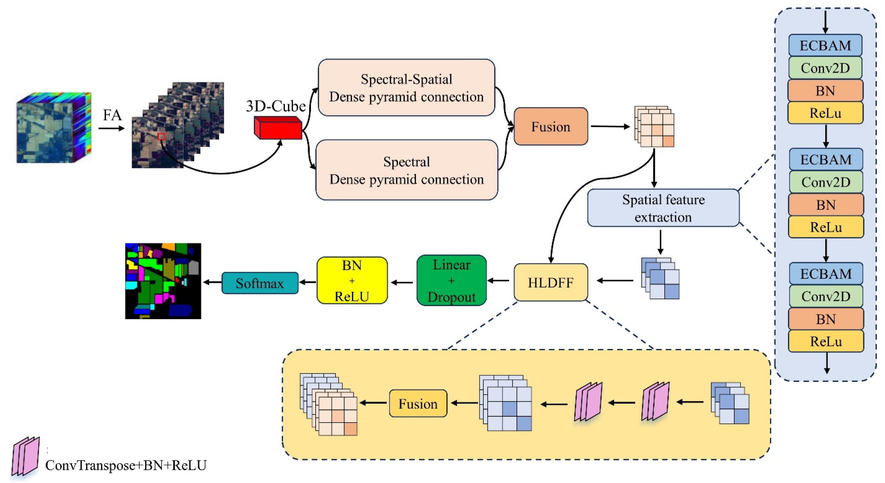
Figure 1 shows the overall design framework of the FHDANet network. The hyperspectral image can be regarded as a high-dimensional data cube, assuming that the spatial dimension of the original hyperspectral data cube is , and the number of spectral bands is , it can be denoted as . The hyperspectral data cube is downscaled using factor analysis (FA), where significant spectral information is retained while the rest of the redundant information and noise are removed, and the overall computation and the number of model parameters are also reduced. The number of spectral bands after FA downscaling is noted as , and the hyperspectral image can be denoted as , which is sliced into patches with the dimensions of , where is the predefined neighbourhood size, the patch category is determined by the category of the central image element, and the patch contains not only the spectral information of the image element to be classified but also the spatial information of the image element within a certain distance around it, and each patch can be denoted as , and the FHDANet takes as input.
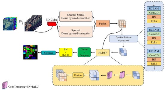
Figure 1.
FHDANet overall framework diagram.
The two-branch dense pyramid structure is a densely connected block composed of 3D-CNNs, and the first branch is the joint spatial–spectrum feature extraction branch, which employs 3D-CNNs with convolutional kernel sizes of , and , respectively, for the joint extraction of multiscale spatial–spectrum information. In this case, dense connections are used to alleviate the gradient vanishing problem, enhance feature propagation, and greatly enhance feature reuse. The second branch is the inter-spectral feature extractor, which also consists of densely connected blocks of 3D-CNN, and differs from the first branch in that its convolutional kernel sizes are , , and in that order, and the focus of the feature extraction is changed from the previous mixed spectral and spatial extraction to the extraction and learning of the spectral information, and the feature maps generated in this branch are fused with those generated from joint spatial–spectral feature extraction The feature maps generated by this branch will be fused with the feature maps generated by spatial–spectrum joint feature extraction.
Let us return to the feature map generated by the first branch. Traditional HyBridSN, including other improved versions, performs feature extraction and learning through a hybrid 3D-2D-CNN, in which spatial and spectral feature learning is performed in the 3D-CNN stage, and spatial correlation learning is performed in the 2D-CNN stage. In the FHDANet proposed in this paper, a branching structure is introduced to make full use of the powerful computational capability of 3D convolution to carry out spatial and spectral feature learning in the spatial–spectrum joint branch and spectral feature learning in the inter-spectrum branch, and finally, the generated feature maps are fused, and the resulting new feature maps serve as input feature maps for the spatial extractor. Adopting the branching structure allows the spectral features to be further extracted and learnt, which is beneficial in the case of small samples, and combined with the dense connectivity mechanism, feature reuse can be well performed.
We introduce an improved efficient channel–spatial block attention module (ECBAM) in the spatial feature extraction stage to efficiently allocate computational resources and enhance the learning of salient spatial features. In addition, we propose a high–low deep feature fusion strategy (HLDFF). HLDFF involves the deconvolution of high-level feature maps generated after convolutional kernel sizes of , and in that order, up-sampling them to the same size as the low-level feature maps, and then splicing the two feature maps together channel-by-channel to obtain a richer representation of the features, thus enhancing feature reuse. Finally, the fully connected layer is used as a classifier to complete the classification task.
2.2. Dense Two-Branch Structure
Given that HSI is a 3D cubic structure with spatial–spectral binding, in 3D convolution, the 3D convolution kernel can be moved in all 3 directions (height, width, and channel of the image). At each position, the multiplication and addition of elements provide a number. Since the filter slides in 3D space, the output digits are also arranged in 3D space, and then the 3D data are output. HSI contains rich one-dimensional spectral information and two-dimensional spatial information; therefore, we adopted 3D-CNN as the convolution module and utilized its excellent computational power as the base building block of the two-branch dense pyramid structure.
In Equation (1), , , and represent the length, width, and number of spectral bands of the 3D convolution kernel, respectively. represents the weights of the kernel that is connected to the th feature cube of the layer; is the activation function.
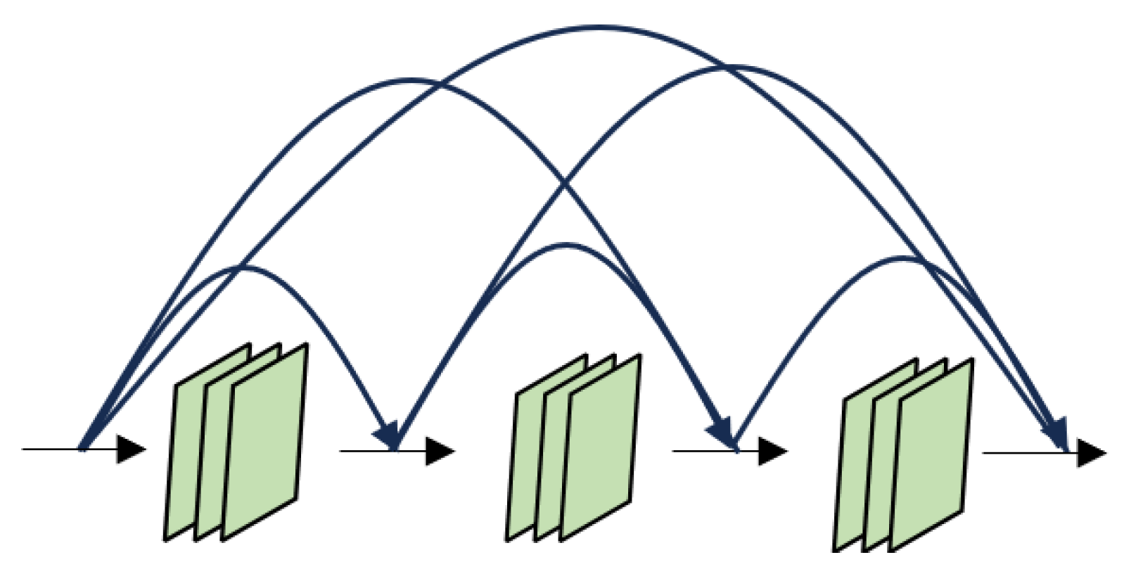
Here, we briefly introduce dense connectivity. DenseNet’s [34] dense connectivity uses feature maps connected in the channel dimension, where each layer is connected to the outputs of all previous layers and serves as an input to the next layer. For a network with layers, it contains connections. Our proposed FHDANet contains two feature feature extractors with a dense pyramid structure, the spatial–spectrum joint dense pyramid feature extractor and the inter-spectrum dense pyramid feature extractor, each of which contains six dense connections, and its feature mapping expression is shown in Equation (2). Introducing the dense connection mechanism into the model makes the model pay more attention to feature reuse and information sharing, enhances the gradient flow, and can substantially improve the performance and generalization ability of the model, although there is a slight loss in computational efficiency. In this paper, we combine the dense connection with 3D-CNN for the construction of dense pyramid structure, which is shown in Figure 2.
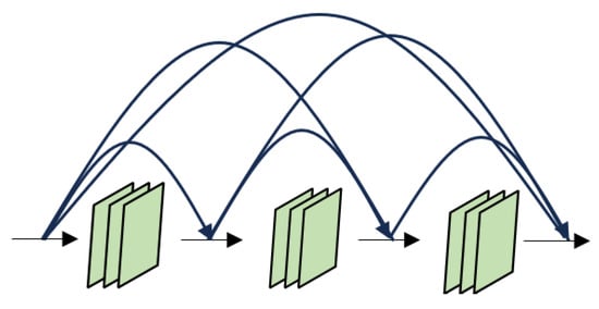
Figure 2.
Schematic diagram of a dense connection.
In Equation (2), denotes the output of layer . Layer receives the feature mapping of the previous layers, and is defined as a composite function of three consecutive operations: Batch normalization (BN), linear rectification unit (ReLU), and 3D convolution.
In the traditional dense connection, researchers mostly default to using the same size of convolutional kernel for feature extraction; however, they ignore an important issue, i.e., the scale problem, and are unable to extract multiscale feature information, which leads to the insufficient feature extraction capability of the model, even though the use of dense connection largely enhances the feature multiplexing but still can not cover up the problem of insufficient feature extraction capabilities. In this paper, we adopted the dense golden tower connection combined with the double branch structure to alleviate the problem of insufficient feature extraction ability of the traditional dense connection.
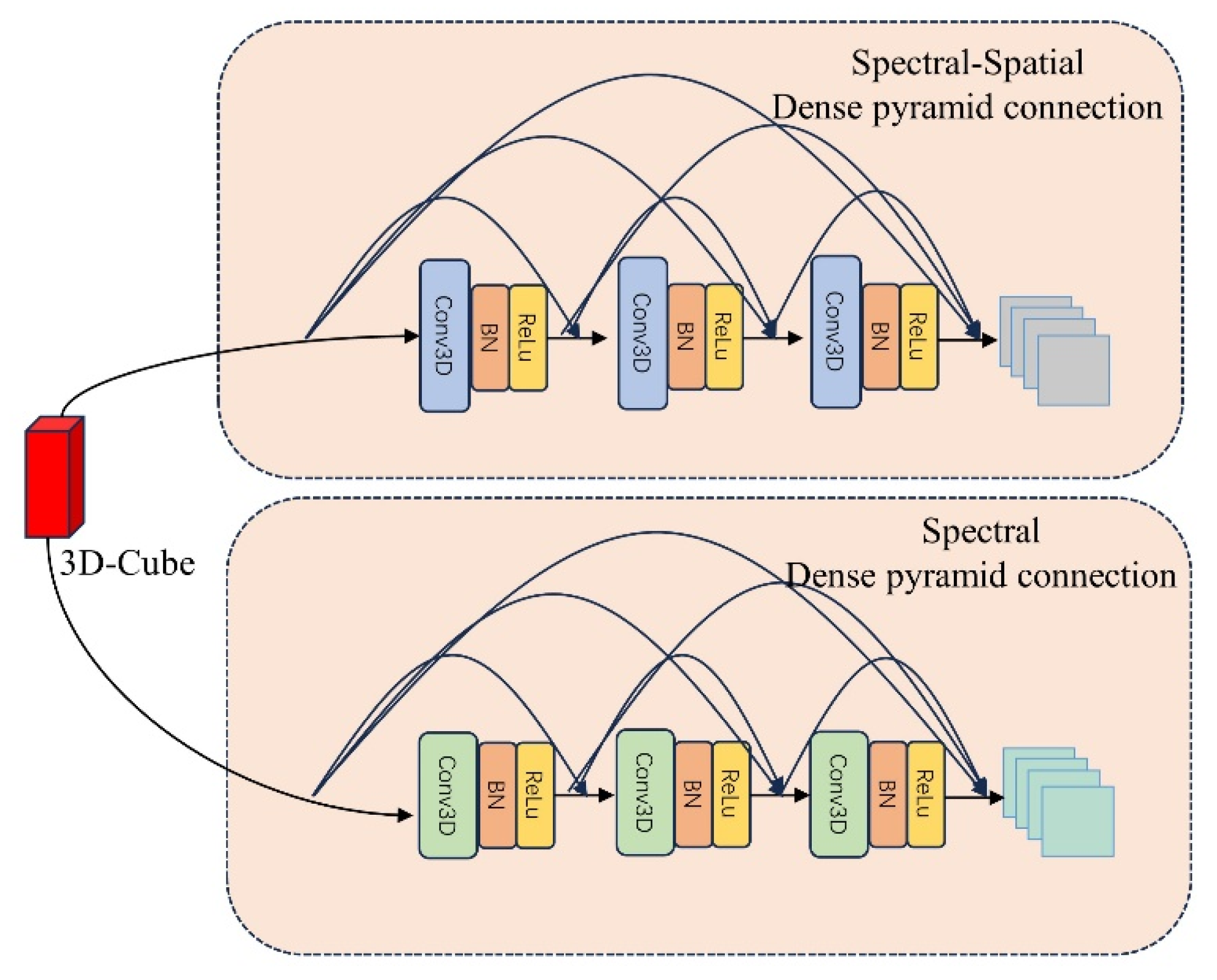
During the dual branch building process, since the size of the output feature maps of each layer varies, the output feature maps of each layer are subjected to maximal pooling to adapt the size of the densely connected feature maps to fit. The spatial–spectrum joint dense pyramid branch, using convolution kernels of size , , in order, uses maximum adaptive pooling for the feature map size of each layer to fit the feature map splicing of each layer to complete the dense connection. The first branch network architecture is shown in Table 1.

Table 1.
Dense pyramid branching architectures of the joint spatial–spectrum.
The inter-spectral dense pyramid branch uses convolution kernels of size 7 × 1 × 1, 5 × 1 × 1, and 3 × 1 × 1 in order, which is consistent with the principle used in the first branch, with maximum adaptive pooling for the feature map size at each layer. The second branch network architecture is shown in Table 2. A schematic diagram of a dense two-branch pyramid connection is shown in Figure 3.
Table 2.
Specific architecture of the joint dense pyramid branch of the spectrum.

Figure 3.
Schematic diagram of a dense two-branch pyramid connection.
2.3. ECBAM Module
In the spatial feature extraction process, we propose an efficient channel–spatial block attention module (ECBAM) focusing on feature extraction for spatial categories of interest while ignoring the influence of background as much as possible. The development of existing mainstream attention modules is centered around two broad aspects: (1) enhanced feature aggregation and (2) the combination of channel and spatial attention. We note that traditional CBAM is divided into two sub-modules, channel, and spatial attention. In the channel attention module, the input feature maps need to be subjected to global maximum pooling and global mean pooling, and subsequently fed into a two-layer neural network, assuming that the number of neurons in the first layer is M/r, and the number of neurons in the second layer is M, the channel attention module performs dimensionality reduction of the original input feature maps. Wang et al. [35] demonstrated, with a large number of experiments in ECA-Net, that dimensionality reduction has a negative effect on the learning ability of the model. Despite the fact it reduces the complexity of the model, it will inevitably lead to information loss, and we should try our best to avoid dimensionality reduction when designing the attention module, and he proposed a local cross-channel interactive attention module ECAM. We are inspired by ECAM and, in this paper, we present the ECBAM attention module on the basis of CBAM.
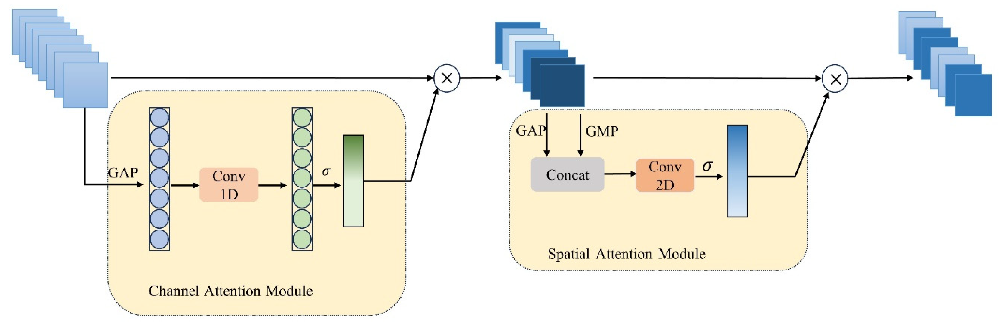
ECBAM consists of two separate sub-modules: the channel attention module and the spatial attention module. In the channel attention module, the convolutional features are aggregated using GAP. We believe that the cross-channel information capturing ability of convolution is very strong; therefore, we used the traditional fully connected layer and instead performed one-dimensional convolution with the convolution kernel size set to 3. Subsequently, the output feature maps are multiplied by the Sigmoid activation function, and finally, the output feature maps are multiplied by the input feature maps to obtain the output feature maps of the channel attention module, as shown in Equation (3). The second module of ECBAM, the spatial attention module, is introduced next. We take the feature maps generated by the channel attention as the input feature maps of this module. The spatial attention module first performs the channel-based global maximum pooling and global mean pooling to connect the respective outputs by the channel dimensions, performs the convolution operation with a convolution kernel of 7, and finally multiplies the output feature maps with the input feature maps to generate the final feature maps . The whole process is shown in Figure 4.
where is the input feature map, is the activation function Sigmoid, is the 1D-CNN with the convolution kernel size of 3, and is global mean pooling.
where is the input feature map, is global maximum pooling, and is the 2D-CNN with the convolution kernel size of 7.

Figure 4.
ECBAM architecture diagram.
2.4. HLDFF Strategy
In order to solve the problem of missing features, in the spatial feature extraction stage, we propose a spatial feature extractor based on the deep feature fusion strategy (HLDFF), which can generate richer and deeper feature representations and enhance the reusability of features in order to improve model performance and generalization ability. In HLDFF, we cleverly use deconvolution to up-sample the high-level feature maps. Deconvolution can greatly recover the spatial feature information lost in the spatial feature extraction process and enhance the feature detail expression ability, so that the resulting high-level feature maps have high spatial accuracy while maintaining rich semantic information. Deconvolution is a special forward convolution process. In this process, the size of the input image is first enlarged by complementing 0 according to a certain ratio, followed by forward convolution.
As shown in Table 3, we use 2D-CNN with convolutional kernel sizes of 7 × 7, 5 × 5, and 3 × 3, and then the extracted high-level feature maps were deconvolutional expanded to the same size as the input low-level feature maps, and then channel-level connectivity was carried out, i.e., the fusion of up-sampled high-level feature maps and low-level feature maps, which not only makes full use of the rich semantic information of high-level feature maps but also combines the fine-grained features of low-level feature maps to construct a more comprehensive and fine-grained feature representation. This fusion process not only makes full use of the rich semantic information of the high-level feature maps but also combines the fine-grained features of the low-level feature maps so as to construct a more comprehensive and fine-grained feature representation. This feature fusion strategy not only enhances the reusability of the features but also improves the ability of the model to capture and utilize the spatial features, which alleviates the problem of spatial feature loss.
Table 3.
Architecture table of HLDFF-based spatial feature extractor.
2.5. Classifier Construction
We use two fully connected layers and Softmax classification loss function for classifier construction, in which the first fully connected layer has the largest number of parameters, and the number of nodes in the last fully connected layer is the same as the number of categories corresponding to the given dataset. In addition, in order to effectively deal with model overfitting due to the large number of model parameters and small number of training samples, Dropout is used to achieve regularization effect to a certain extent to alleviate the occurrence of overfitting; ReLU is chosen as the nonlinear activation function; and BN layers are added after each convolutional layer to make the training easier and accelerate the convergence.
3. Experimental Analysis
3.1. Introduction of the Dataset
To evaluate the classification performance of FHDANet, we used four datasets with fewer training samples, namely: the Indian Pines Dataset (IP), Pavia University Dataset (PU), Kennedy Space Center Dataset (KSC), and the Salinas Dataset (SA).
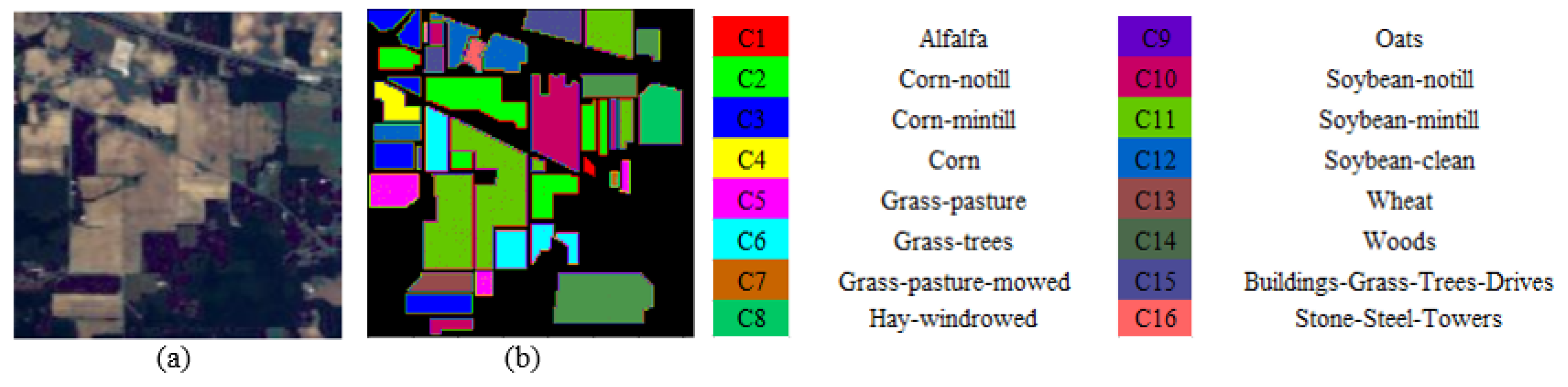
IP: The scene was collected using an airborne visible/infrared imaging spectrometer (AVIRIS) at IP Proving Ground, NW India. It contains 145 145 pixels, 224 spectral bands in the wavelength range of 0.4 to 2.5 μm. Then, 24 of the spectral bands were removed due to water absorption and damage. The reference feature targets were designed as 16 vegetation classes. As shown in Figure 5.
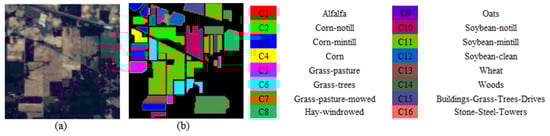
Figure 5.
Visualization of the classification maps for the IP dataset: (a) Three-band false color composite; (b) ground truth.
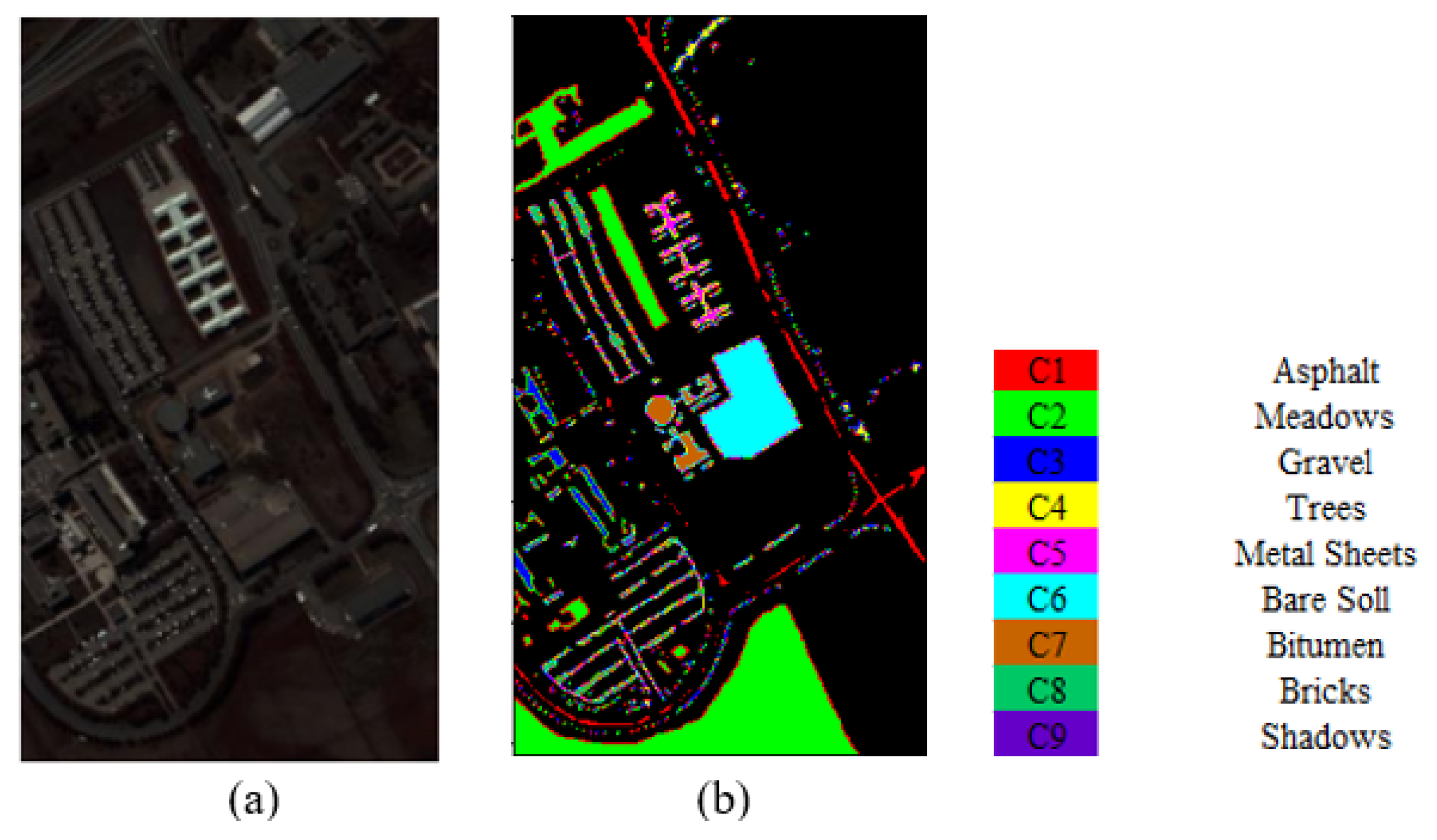
PU: The scene was acquired using a reflectance optical system imaging spectrometer (ROSIS) during a flight campaign over PU in 2001. The wavelength range is 0.43 to 0.86 μm. The dataset presents the ground scene in a 610 340 image format with a spatial resolution of 1.3 m per pixel and contains nine types of urban land cover classes. As shown in Figure 6.

Figure 6.
Visualization of the classification maps for the PU dataset: (a) three-band false color composite; (b) ground truth.
KSC: The KSC dataset was captured by the Kennedy Space Center in Florida in 1996 using the AVIRIS imaging spectrometer. AVIRIS collected 224 bands of 10 nm width with a centre wavelength of 400–2500 nm. The KSC dataset was analyzed with a spatial resolution of 18 m using 176 bands after removing the absorbing and low signal-to-noise back bands. The dataset has a spatial dimension of 512 614 pixels and contains a total of 5211 samples across 13 categories. As shown in Figure 7.

Figure 7.
Visualization of the classification maps for the KSC dataset: (a) three-band false color composite; (b) ground truth.
SA: The dataset was acquired by the AVIRIS sensor (224 bands) over the SA Valley, California, USA, with a spatial resolution of 3.7 m. The coverage scene is presented in 512 rows and 217 columns of pixels, and 20 absorbing and noisy spectral bands have been discarded. The feature targets in this dataset totaled 16 categories. As shown in Figure 8.
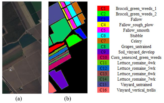
Figure 8.
Visualization of the classification maps for the SA dataset: (a) three-band false color composite; (b) ground truth.
3.2. Experimental Design
We use three performance metrics to evaluate the performance of the model, which are overall classification accuracy (OA), average accuracy (AA) and kappa (κ), where OA calculates the ratio of correctly classified samples to all the samples in the test set, AA is used to determine the average classification accuracy across all the classes, and at the same time, it can be a good assessment of the classification results of the classes with fewer training samples, and confusion-based κ calculated from the confusion matrix indicates how well the classification labels obtained by the classification model match the ground truth labels.
In order to verify the excellence of FHDANet, we compared the FHDANet model with SVM [8], SSRN [36], HyBridSN, LANet [37], A2S2K-ResNet, SSDGL [38], and RSSGL [39] classification networks. To ensure the fairness of the experimental results, all methods use the same parameters as presented in the authors’ published paper. Some of the deep learning methods share spatial patch sizes and dimensions, while SVM uses serialized data. We take full account of the large differences between the four datasets, so our experiments take the form of a differentiated dataset division. In the IP and KSC datasets, we selected 5% as the training and validation sets and the rest as the test set; in the SA and PU datasets, we selected and retained 1% as the training set and the rest as the test set. All of the experiments were run on an Intel Core i7-13700KF processor and NVIDIA GeForce RTX 4090 graphics card. The programming language used was Python. The classification network was built using PyTorch, and PyCharm was used as the compiler. The batch size was set to 32. Adam was used as the optimizer, and the learning rate was set to 0.001. We set up random seeds before the experiment and used them to ensure the reproducibility of the results.
3.3. Classification Maps and Categorized Results
3.3.1. Classification Maps and Categorized Results for the IP Dataset
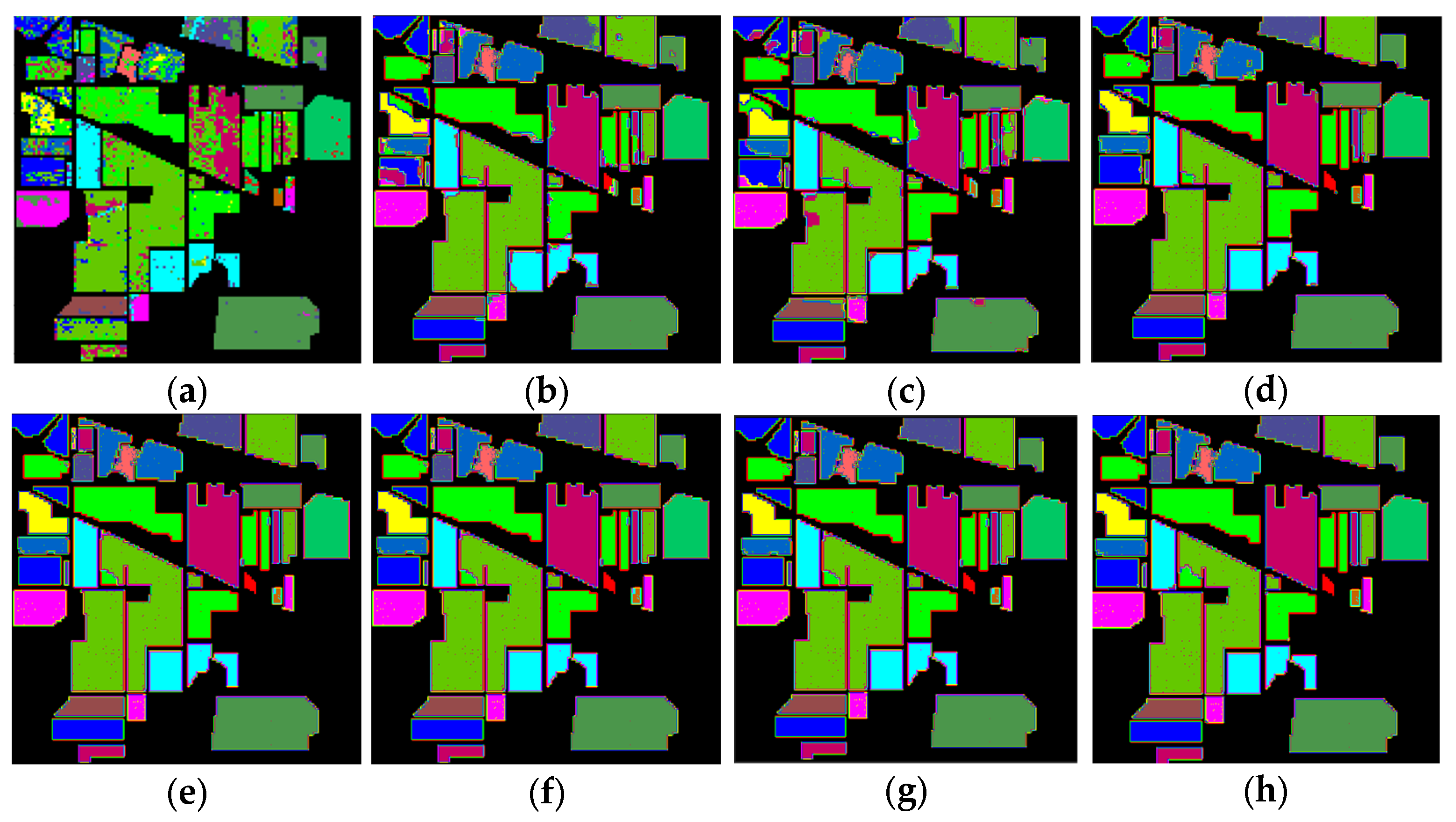
The experiments were conducted on the IP dataset, and the table shows the overall accuracy (OA), average accuracy (AA) and kappa () of different classification methods, as well as the classification performance metrics for each category. The visualization results of all the methods are shown in Figure 9. From Table 4, it can be seen that in the IP dataset, the classification accuracy (OA) of SVM is 73.26%, while other deep learning-based classification methods, their OA is more than 90%. The OA of SSRN, A2S2K-ResNet, HyBridSN, SSDGL, RSSGL, and LANet is 92.85%, 94.35%, 92.18%, 96.84%, 96.37%, 95.40%, respectively. FHDANet, proposed in this paper, has an OA of 99.76%, which is 6.91%, 5.41%, 7.58%, 2.92%, 3.39%, and 4.36% higher than the OA of other deep learning-based methods, respectively, and it shows very excellent classification performance. In addition, the classification accuracies of each category exceeded 98%, which are all better than other deep learning-based classification models.
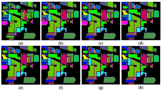
Figure 9.
Classification maps produced using the different methods for the IP dataset: (a) SVM, (b) SSRN, (c) A2S2K-ResNet, (d) HyBridSN, (e) SSDGL, (f) RSSGL, (g) LANet, and (h) FHDANet.
Table 4.
Comparison of the different methods in terms of class accuracy, OA, AA, and for the IP dataset.
3.3.2. Classification Maps and Categorized Results for the PU Dataset
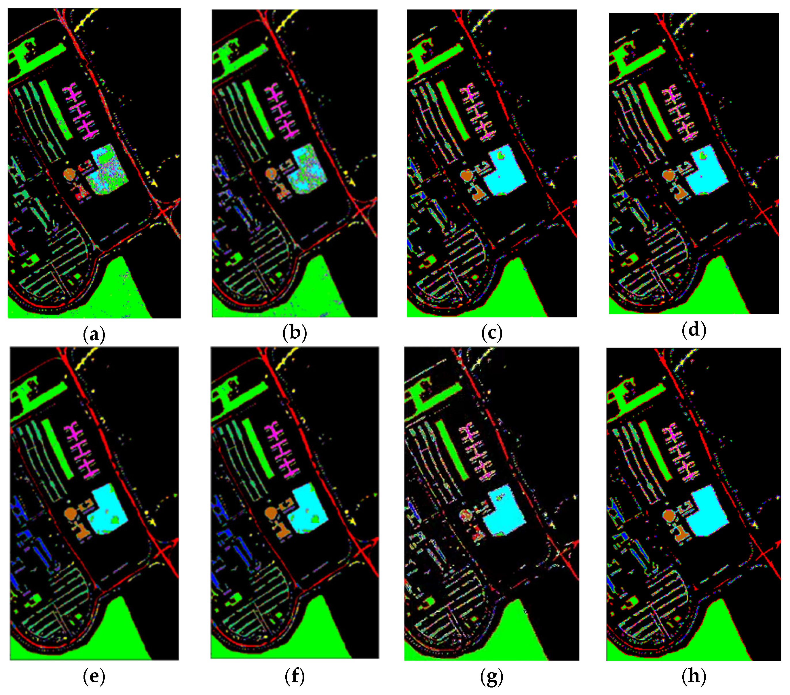
The experiment was conducted on the PU dataset. Table 5 and Figure 10 show the classification performance metrics of different methods and the classification effect graph of different methods, respectively. The OA of SSRN, A2S2K-ResNet, HyBridSN, SSDGL, RSSGL, and LANet is 86.44%, 93.24%, 92.68%, 97.65%, 98.35%, and 93.28%, respectively. Our proposed model FHDANet in this paper has an OA of 98.38%, which is 11.94%, 5.14%, 5.7%, 0.73%, 0.03% and 5.1% higher than the OA of other deep learning-based methods, respectively, and it shows very excellent classification performance. The classification accuracy of each category is also above 90%. Compared to the high accuracy achieved in the other feature categories, the classification accuracy of the shadows category is only 90.12%, which is significantly lower than the other categories. The possible reason is that the training samples are too small, which results in very little feature information extracted during the training period.
Table 5.
Comparison of the different methods in terms of class accuracy, OA, AA, and for the PU dataset.
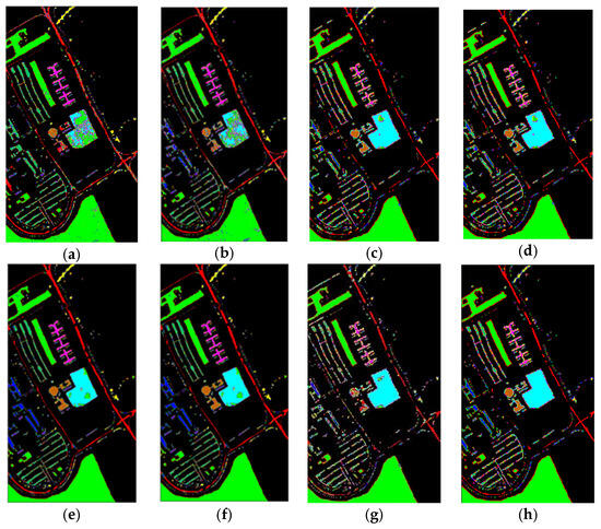
Figure 10.
Classification maps produced by the different methods for the PU dataset: (a) SVM, (b) SSRN, (c) A2S2K-ResNet, (d) HyBridSN, (e) SSDGL, (f) RSSGL, (g) LANet, and (h) FHDANet.
3.3.3. Classification Maps and Categorized Results for the KSC Dataset
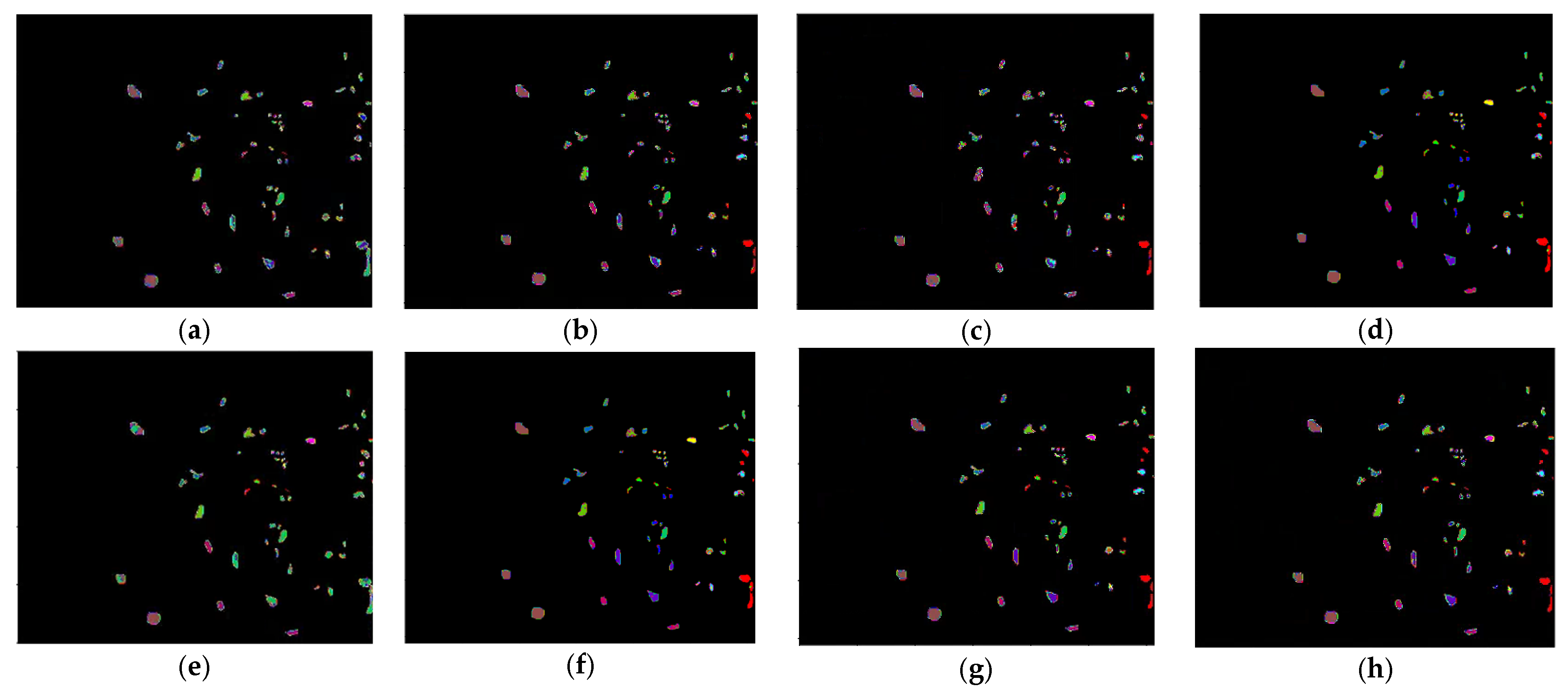
This experiment was conducted on the KSC dataset. Table 6 and Figure 11 show the classification performance metrics of the different methods and the classification effect graphs of the different methods, respectively. The OA of FHDANet is 97.09%, the AA is 95.92, and the is 0.96, and its OA is higher than that of the SSRN, A2S2K-ResNet, HyBridSN, SSDGL, RSSGL, and LANet classification models: 5.55%, 0.23%, 3.59%, 4.29%, 2.93% and 0.47%, respectively.
Table 6.
Comparison of the different methods in terms of class accuracy, OA, AA, and for the KSC dataset.
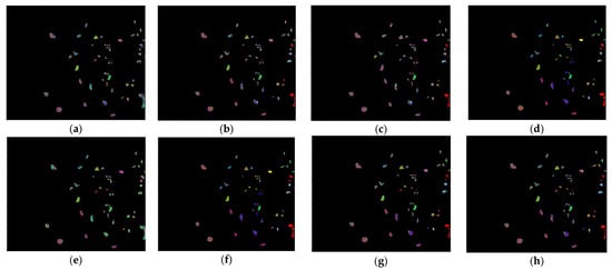
Figure 11.
Classification maps produced by the different methods for the KSC dataset: (a) SVM, (b) SSRN, (c) A2S2K-ResNet, (d) HyBridSN, (e) SSDGL, (f) RSSGL, (g) LANet, and (h) FHDANet.
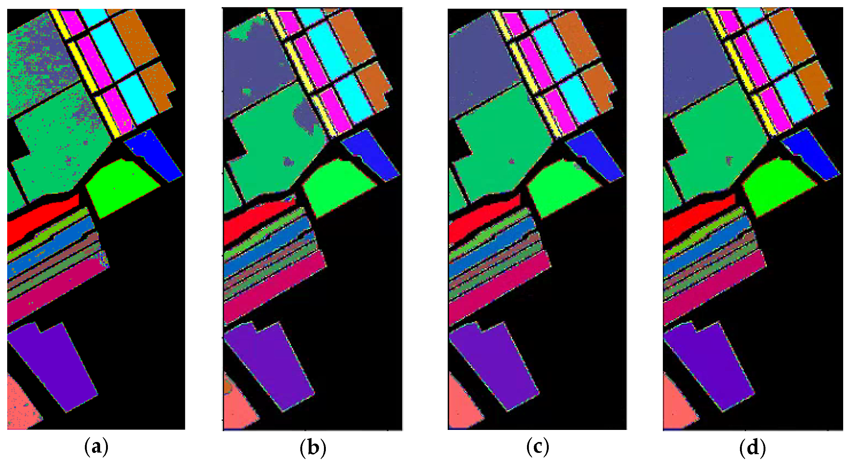
3.3.4. Classification Maps and Categorized Results for the SA Dataset
This experiment was conducted on the SA dataset. Table 7 and Figure 12 show the classification performance metrics of different methods and the classification effect graphs of different methods, respectively. The OA of FHDANet is 99.08%, the AA is 99.14%, and the κ is 0.98, and its OA is higher than that of the SSRN, A2S2K-ResNet, HyBridSN, SSDGL, RSSGL, and LANet classification models: 5.47%, 2.24%, 0.58%, 1.17%, 0.64%, and 3.52%, respectively. The classification accuracy of each feature class is above 97%, and the classification performance is significantly better than the other compared algorithms.
Table 7.
Comparison of the different methods in terms of class accuracy, OA, AA, and for the SA dataset.
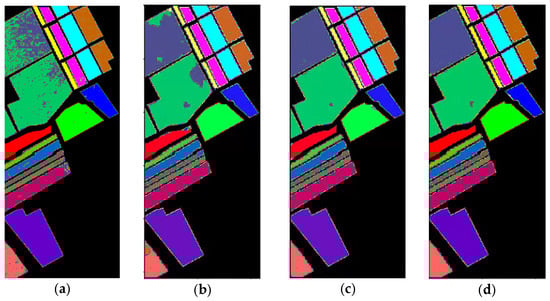
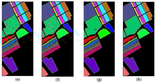
Figure 12.
Classification maps produced by the different methods for the SA dataset: (a) SVM, (b) SSRN, (c) A2S2K-ResNet, (d) HyBridSN, (e) SSDGL, (f) RSSGL, (g) LANet, and (h) FHDANet.
3.4. Ablation Experiment
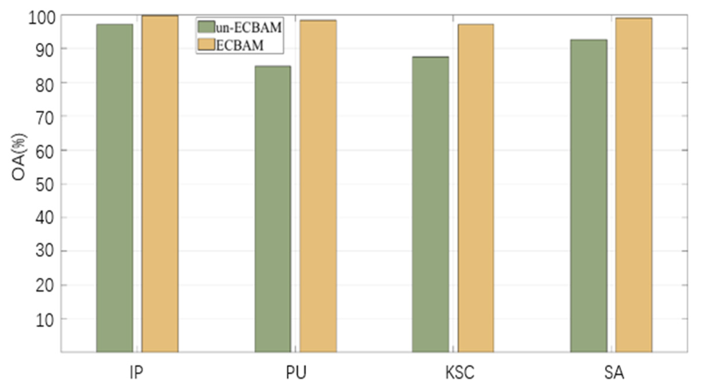
In order to verify the effectiveness of ECBAM, the channel–spatial attention module proposed in this paper, we conducted ablation experiments on four representative datasets. As shown in Table 8 and Figure 13, on the four datasets, OA increased by an average of 8.05%, and even more so on the PU dataset, which increased by 13.57%, AA increased by an average of 11.47%, and increased by an average of 0.1. The results of the ablation experiments proved the effectiveness of ECBAM, and the incorporation of the ECBAM module in the model can significantly enhance the performance of model classification.
Table 8.
Effect of ECBAM on four HSI datasets.
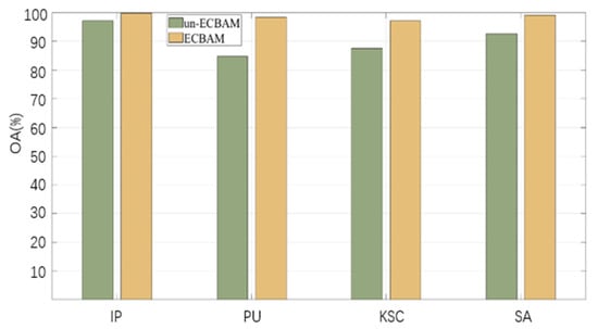
Figure 13.
Effect of ECBAM on four HSI dataset.
3.5. Analysis of the Parameter Effect
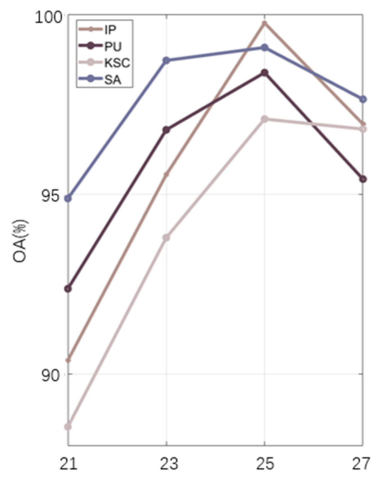
The patch block size of an image is one of the most important hyperparameters in the model. Its impact on the classification performance of the model is significant because the size of the patch window determines the abundance of spatial information extracted from the patches, and according to the inherent experience, the larger the size of the patch window, the richer the spatial information extracted, and thus, the higher the classification performance of the model. However, if the patch window is too large, it will lead to the data overlapping problem, decreasing the classification performance of the model. In order to evaluate the effect of the size of the image patches on the performance of the FHDANet model, we set the window size of the patches to 21 × 21, 23 × 23, 25 × 25, 27 × 27; the OA of the model is used as the evaluation criterion. As shown in the Figure 14, we clearly found that as the window size of the patch increased, the obtained OA increased, proving that the classification accuracy gradually increases; however, when the OA reaches the peak, we found that the window size is 25 × 25 at this time, proving that the window size applicable to the present model is 25 × 25. In addition, we also found that when the window size increases, the classification accuracy of the model firstly increases and then decreases. In summary, for all the experiments in this paper, we take the optimal patch window size of 25 × 25.
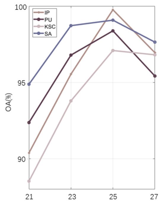
Figure 14.
Classification performance of different input patch sizes on four datasets.
3.6. Evaluation of Model Complexity
We compared the computational costs of the different methods on the IP dataset, with a special focus on the size of the model’s training parameter scale, the number of floating-point operations, and the training time, as shown in Table 9. We found that the training time of the deep learning-based model is higher than that of the traditional machine learning algorithm, SVM. while the training time of RSSGL is much higher than that of the other comparative algorithms, which may be due to the fact that (1) RSSGL is a global learning framework, and the computational complexity will be higher compared to other models; (2) ConvLSTM uses three-dimensional convolutional techniques, resulting in a significant increase in the number of floating-point operations, which leads to higher computational costs. A2S2K-ResNet and HyBridSN use three-dimensional convolutional techniques internally, which leads to higher FLOP values. The FHDANet proposed in this paper uses a dense pyramid connection consisting of the 3D convolution technique as a feature extractor. This leads to a higher FLOP value, and hence, longer training time. However, the advantages of using the dense pyramid structure are self-evident, and the classification accuracy of FHDANet is significantly better than other comparative algorithms. In conclusion, our proposed FHDANet exhibits the best performance for each of the same parameters.
Table 9.
Comparison of computational costs of different models on the IP dataset.
4. Discussion
In this paper, we propose a hyperspectral image classification model FHDANet based on a dense two-branch structure. In FHDANet, we propose a new spatial–channel attention module ECBAM and a spatial feature extractor based on a deep feature fusion strategy (HLDFF). In the model, we adopt a dense two-branch connection structure for the construction of the joint spatial–spectral feature extractor and the inter-spectral feature extractor, which alleviates the problems of feature loss and insufficient feature extraction caused by the use of traditional methods, increases the feature reuse, and better obtains the spatial–spectral context information. In order to better cope with the problems of “same object, different spectrum” and “different object, same spectrum”, we adopt multiscale pyramid connection to carry out multiscale feature extraction so as to better combine the spatial feature information. Meanwhile, in the process of constructing the spatial feature extractor, we innovatively propose HLDFF to further enhance the feature reuse, and HLDFF can generate richer and deeper feature expressions through the clever use of deconvolution to enhance the feature reuse, in order to improve the model performance and generalization ability. In addition, we propose the ECBAM attention module, which uses the global mean pooling kernel 1DCNN for feature aggregation, directly avoiding the feature loss caused by the dimensionality reduction in the traditional attention module. Meanwhile, in order to better mitigate the effects of “same object, different spectrum” and “different object, same spectrum”, we use ECBAM to maintain the model’s sensitivity to salient features so as to better incorporate spatial contextual information and improve classification accuracy. The above experiments on the four datasets demonstrate that FHDANet possesses excellent classification performance. The six deep learning-based classification models, SSRN, A2SK2-ResNet, HyBridSN, SSGDL, RSSDL, and LANet, which were compared, all share a common defect, that is, they fail to consider the problems of feature loss and insufficient feature extraction ability well and ignore feature reuse to a certain extent. In the case of sufficient training samples, these problems can be masked, but when in the condition of few training samples, the limitations of these methods are exposed. In addition to this, each comparison model has its shortcomings, which will be analyzed in detail for the overall classification performance in the following. Looking at the model as a whole, the modular design allows for good scalability, specifically by performing operations such as adding or replacing new network layers, meaning that loss functions or optimizers can be changed relatively easy.
As shown in Figure 9, Figure 10, Figure 11 and Figure 12 and Table 4, Table 5, Table 6 and Table 7, in A2S2K-ResNet, a large amount of labeled data are required, the limitations of the model are exposed under small sample conditions, and the risk of overfitting is greatly increased, so its accuracy is much smaller than that of the FHDANet proposed in this paper on all four datasets, with gaps of 5.41%, 5.14%, 0.23%, and 2.24%, respectively. The network structure of SSRN is more complex. This leads to similar drawbacks as those seen in A2S2K-ResNet, i.e., a large amount of labeled data are required, which would otherwise lead to the risk of overfitting, but due to the large number of spectral residual blocks and spatial residual blocks inside the model, the model not only mitigates the risk of gradient vanishing and overfitting but also achieves feature reuse to a certain degree, which mitigates the problem of feature loss, and thus, the average OA of the four datasets reaches 91.13%. Although HyBridSN attaches importance to multiscale feature extraction and distinguishes between spatial and spatial–spectral information extraction, it ignores the problem of feature loss, and thus, performs better in the experiments, and the OA even reaches 98.57% in the SA dataset, which confirms that multiscale feature information extraction is beneficial to the model in terms of improving the generalization ability, and thus, the overall classification performance. In SSGDL and RSSGL, since they are actually global feature extraction frameworks, and despite the fact that they have slightly greater accuracy than several other comparison algorithms, they have high computational costs, involve large FLOP values, and are not effective overall. In LANet, the classification effect is not as good as that of FHDANet in this paper due to the fact that it does not consider the joint multiscale spatial–spectral information. From the ablation experiments, as shown in Table 8, the addition of the ECBAM module can better ensure the model’s saliency feature extraction ability, thus enhancing the model’s generalization ability. As shown in Figure 9, Figure 10, Figure 11 and Figure 12 and Table 4, Table 5, Table 6 and Table 7, we can see that when the model is trained and tested using four different datasets, we find that both in terms of the classification accuracy of individual categories and the overall classification accuracy, our proposed FHDANet model is significantly improved compared with previous deep learning algorithms, which shows that the model is highly robust in relation to different datasets.
Let us go back to the two-branch dense concatenation mechanism. Dense concatenation not only improves the reusability of features but, more importantly, it alleviates the problem of gradient vanishing as the model depth deepens. As shown in the figure, the parameter sharing between different layers of the dense concatenation greatly reduces the amount of parameter training in terms of the network but undeniably increases the amount of gradient information that needs to be computed, which leads to an increase in the value of the model’s FLOPs, which is intuitively manifested as an increase in the training time of the model. However, we can reduce the number of convolutional layers by means of dense connectivity, making the depth of the network considerably lower, and from this point of view, dense connectivity can be considered as an indispensable and fundamental mechanism to improve the generalization of the model, at least as far as FHDANet is concerned.
5. Conclusions
In this paper, we propose a highly accurate two-branch multiscale feature aggregation and multiple attention mechanism for hyperspectral image classification model FHDANet. The model achieves high efficiency extraction of spatial–spectral and inter-spectral feature information by using dense two-branch pyramid connection, which largely reduces feature loss and strengthens the model’s ability to extract contextual information; we propose a channel–space attention module, ECBAM, which greatly improves the extraction capability of the model for salient features. A spatial information extraction module based on the deep feature fusion strategy HLDFF is proposed, which fully strengthens the feature reuse capability and mitigates the feature loss problem brought about by the deepening of the model. Experiments were carried out on four representative datasets, and the experiments proved that FHDANet has excellent classification performance under the condition of small samples, which is better than other comparative experiments.
However, our proposed model still has some shortcomings. First, as far as the dimensionality reduction in the preprocessing step of the HSI is concerned, we used FA to perform dimensionality reduction on the HSI in order to reduce the computational complexity of the model. However, no matter how dimensionality reduction is used, it will lead to the unavoidable loss of information in the original HSI, which is a source loss and we cannot recover it by means of dense joining, residual joining, and inverse convolution, etc. Therefore, the model’s future development should be optimized in the direction of full-band feature extraction. Specifically, we should try our best to solve the problem caused by Hughes phenomenon, i.e., the phenomenon that classification accuracy increases and then decreases with the increase in the number of bands involved in the operation. Secondly, the proposed model is a 3D-2D-CNN model based on dense two-branch pyramid connection, which can effectively improve the classification performance and obtain high-precision classification results; however, the large number of floating-point operations leads to an increase in the training time of the model, which makes the model less computationally efficient.
In addition, under small sample conditions, we should think that, in addition to deepening the depth of the network and using feature reuse, there is a more direct way to cope with the phenomenon of low classification accuracy brought about by the use of small samples, and this research method is how to give full play to and make use of the value of a large number of unlabeled samples under the condition of given labeled samples so as to enable the classification model to fully exert its potential to obtain optimal generalization performance, which is also commonly known as semi-supervised algorithm research. This is also commonly known as semi-supervised algorithm research. The optimization direction of the model should be toward semi-supervision to take advantage of the large amount of unlabeled data because simply deepening the network and performing feature reuse will make the model consume a huge amount of computational resources; however, using semi-supervised methods can take advantage of the large amount of unlabeled samples; specifically, we do not need to overemphasize feature reuse in the design of the network. Firstly, a small number of labeled samples are used for the model. First, the model is pre-trained using a small number of labeled samples; second, the model is used to generate pseudo-labels for the unlabeled samples, and then the model is co-trained using both labeled and pseudo-labeled samples. This classification model based on pseudo-label generation can make full use of the feature information in hyperspectral data to a great extent, while saving computational resources to a certain extent. Overall, the future optimization direction of the model should be towards full-waveband and semi-supervised direction so as to further improve the robustness and generalization ability of the model.
Author Contributions
Conceptualization, L.W.; Methodology, B.M.; Writing—review & editing, H.W. All authors have read and agreed to the published version of the manuscript.
Funding
This research was funded by the National Natural Science Foundation of China (Grant No. 62071084) and the Fundamental Research Funds for the Central Universities (grant number 04442024040 and 04442024041).
Data Availability Statement
All datasets can be obtained at http://www.ehu.eus/ccwintco/index.php?title=Hyperspectral_Remote_Sensing_Scenes (accessed on 20 May 2011).
Conflicts of Interest
The authors declare no conflicts of interest.
References
- Huang, H.; Zheng, X.L. Hyperspectral image classification based on weighted spatial-spectral and nearest neighbor classifier. Opt. Precis. Eng. 2016, 24, 873–881. [Google Scholar] [CrossRef]
- Lee, M.A.; Huang, Y.; Yao, H.; Thomson, S.J.; Bruce, L.M. Determining the effects of storage on cotton and soybean leaf samples for hyperspectral analysis. IEEE J. Sel. Top. Appl. Earth Obs. Remote Sens. 2014, 7, 2562–2570. [Google Scholar] [CrossRef]
- Dalponte, M.; Ørka, H.O.; Gobakken, T.; Gianelle, D.; Næsset, E. Tree species classification in boreal forests with hyperspectral data. IEEE Trans. Geosci. Remote Sens. 2013, 51, 2632–2645. [Google Scholar] [CrossRef]
- Yuan, Y.; Wang, Q.; Zhu, G. Fast hyperspectral anomaly detection via High-Order 2-D crossing filter. IEEE Trans. Geosci. Remote Sens. 2014, 53, 620–630.5. [Google Scholar] [CrossRef]
- Zhang, L.; Zhang, L.; Tao, D.; Huang, X.; Du, B. Hyperspectral remote sensing image subpixel target detection based on supervised metric learning. IEEE Trans. Geosci. Remote Sens. 2014, 52, 4955–4965. [Google Scholar] [CrossRef]
- Zhang, B.; Wu, D.; Zhang, L.; Jiao, Q.; Li, Q. Application of hyperspectral remote sensing for environment monitoring in mining areas. Environ. Earth Sci. 2012, 65, 649–658. [Google Scholar] [CrossRef]
- Camps-Valls, G.; Tuia, D.; Bruzzone, L.; Benediktsson, J.A. Advances in hyperspectral image classification: Earth monitoring with statistical learning methods. IEEE Signal Process. Mag. 2013, 31, 45–54. [Google Scholar] [CrossRef]
- Hou, P.H.; Yao, M.L.; Ja, W.M. Classification of hyperspectral images with spatial structure preservation. Infrared Laser Eng. 2017, 46, 1228001–1228008. [Google Scholar]
- Melgani, F.; Bruzzone, L. Classification of hyperspectral remote sensing images with support vector machines. IEEE Trans. Geosci. Remote Sens. 2004, 42, 1778–1790. [Google Scholar] [CrossRef]
- Krizhevsky, A.; Sutskever, I.; Hinton, G. ImageNet Classification with Deep Convolutional Neural Networks. Adv. Neural Inf. Process. Syst. 2012, 25. [Google Scholar] [CrossRef]
- Simonyan, K.; Zisserman, A. Very deep convolutional networks for large-scale image recognition. arXiv 2014, arXiv:1409.1556. [Google Scholar]
- Hu, W.; Huang, Y.; Wei, L.; Zhang, F.; Li, H. Deep convo-lutional neural networks for hyperspectral image classifi-cation. J. Sens. 2015, 2015, 258619. [Google Scholar] [CrossRef]
- Yue, J.; Zhao, W.; Mao, S.; Liu, H. Spectral-spatial classification of hyperspectral images us-ing deep convolutional neural networks. Remote Sens. Lett. 2015, 6, 468–477. [Google Scholar] [CrossRef]
- Zhao, S.; Li, W.; Du, Q.; Ran, Q. Hyperspectralclassification based on Siamese neural network usingspectral-spatial feature. In Proceedings of the IGARSS 2018—2018 IEEE In-ternational Geoscience and Remote Sensing Symposium, Valencia, Spain, 22–27 July 2018; IEEE: Piscataway, NJ, USA, 2018; pp. 2567–2570. [Google Scholar]
- Wu, S.; Zhang, J.; Zhong, C. Multiscale spectral-spatial unified networks for hyperspectral image classification. In Proceedings of the IGARSS 2019—2019 IEEE Intertional Geoscience and Remote Sensing Symposium, Yokohama, Japan, 28 July–2 August 2019; IEEE: Piscataway, NJ, USA, 2019; pp. 2706–2709. [Google Scholar]
- Chen, Y.; Jiang, H.; Li, C.; Jia, X.; Ghamisi, P. Deep feature extraction and classification of hyperspectral images based on convolutional neural networks. IEEE Trans. Geosci. Remote Sens. 2016, 54, 6232–6251. [Google Scholar] [CrossRef]
- Santara, A.; Mani, K.; Hatwar, P.; Singh, A.; Garg, A.; Padia, K.; Mitra, P. Bass Net: Band-adaptive spectral-spatial feature learning neural network for hyperspectral image classification. IEEE Trans. Geosci. Remote Sens. 2017, 55, 5293–5301. [Google Scholar] [CrossRef]
- Audebert, N.; Saux, B.L.; Lefevre, S. Deep learning for classification of hyperspectral data: A comparative review. IEEE Geosci. Remote Sens. Mag. 2019, 7, 159–173. [Google Scholar] [CrossRef]
- Li, X.; Ding, M.; Pižurica, A. Deep feature fusion via two-stream convolutional neural network for hyperspectral image classification. IEEE Trans. Geosci. Remote Sens. 2020, 58, 2615–2629. [Google Scholar] [CrossRef]
- Xi, B.; Li, J.; Li, Y.; Song, R.; Shi, Y.; Liu, S.; Du, Q. Deep prototypical networks with hybrid residual attention for hyperspectral image classification. IEEE J. Sel. Top. Appl. Earth Obs. Remote Sens. 2020, 13, 3683–3700. [Google Scholar] [CrossRef]
- Roy, S.K.; Krishna, G.; Dubey, S.R.; Chaudhuri, B.B. HybridSN: Exploring 3-D–2-D CNN Feature Hierarchy for Hyperspectral Image Classification. IEEE Geosci. Remote Sens. Lett. 2020, 17, 277–281. [Google Scholar] [CrossRef]
- Zhang, M.; Li, W.; Du, Q. Diverse Region-Based CNN for Hyperspectral Image Classification. IEEE Trans. Image Process. 2018, 27, 2623–2634. [Google Scholar] [CrossRef]
- Roy, S.K.; Manna, S.; Song, T.; Bruzzone, L. Attention-based adaptive spectral–spatial kernel ResNet for hyperspectral image classification. IEEE Trans. Geosci. Remote Sens. 2021, 59, 7831–7843. [Google Scholar] [CrossRef]
- Pu, Y.; Wang, Y.; Xia, Z.; Han, Y.; Wang, Y.; Gan, W.; Wang, Z.; Song, S.; Huang, G. Adaptive Rotated Convolution for Rotated Object Detection. In Proceedings of the IEEE/CVF International Conference on Computer Vision (ICCV), Paris, France, 2–6 October 2023. [Google Scholar]
- Yang, L.; Chen, Y.; Song, S.; Li, F.; Huang, G. Deep Siamese Networks Based Change Detection with Remote Sensing Images. Remote Sens. 2021, 13, 3394. [Google Scholar] [CrossRef]
- Scheibenreif, L.; Mommert, M.; Borth, D. Masked Vision Transformers for Hyperspectral Image Classification. In Proceedings of the IEEE/CVF Conference on Computer Vision and Pattern Recognition, Vancouver, BC, Canada, 18–22 June 2023. [Google Scholar]
- Zhang, H.K.; Li, Y.; Jiang, Y.N. Research status and prospect of in-depth learning in hyperspectral image classification. Acta Autom. 2018, 44, 961–977. (In Chinese) [Google Scholar]
- Chen, Y.; Lin, Z.; Zhao, X.; Wang, G.; Gu, Y. Deep learning-based classification of hyperspectral data. IEEE J. Sel. Top. Appl. Earth Obs. Remote Sens. 2014, 7, 2094–2107. [Google Scholar] [CrossRef]
- Feng, F.; Wang, S.; Wang, C.; Zhang, J. Learning Deep Hierarchical Spatial–Spectral Features for Hyperspectral Image Classification Based on Residual 3D-2D CNN. Sensors 2019, 19, 5276. [Google Scholar] [CrossRef]
- Zhang, J.; Zhao, L.; Jiang, H.; Shen, S.; Wang, J.; Zhang, P.; Zhang, W.; Wang, L. Hyperspectral Image Classification Based on Dense Pyramidal Convolution and Multi-Feature Fusion. Remote Sens. 2023, 15, 2990. [Google Scholar] [CrossRef]
- Yu, C.; Han, R.; Song, M.; Liu, C.; Chang, C.I. Feedback attention-based dense CNN for hyperspectral image classification. IEEE Trans. Geosci. Remote Sens. 2021, 60, 5501916. [Google Scholar] [CrossRef]
- Woo, S.; Park, J.; Lee, J.Y.; Kweon, I.S. Cbam: Convolutional block attention module. In Proceedings of the European Conference on Computer Vision (ECCV), Munich, Germany, 8–14 September 2018; pp. 3–19. [Google Scholar]
- Ma, W.; Yang, Q.; Wu, Y.; Zhao, W.; Zhang, X. Double-branch multi-attention mechanism network for hyperspectral image classification. Remote Sens. 2019, 11, 1307. [Google Scholar] [CrossRef]
- Huang, G.; Liu, Z.; Van Der Maaten, L.; Weinberger, K.Q. Densely Connected Convolutional Networks. In Proceedings of the 2017 IEEE Conference on Computer Vision and Pattern Recognition (CVPR), Honolulu, HI, USA, 21–26 July 2017; pp. 2261–2269. [Google Scholar]
- Wang, Q.; Wu, B.; Zhu, P.; Li, P.; Zuo, W.; Hu, Q. ECA-Net: Efficient Channel Attention for Deep Convolutional Neural Networks. In Proceedings of the 2020 IEEE/CVF Conference on Computer Vision and Pattern Recognition (CVPR), Seattle, WA, USA, 14–19 June 2020. [Google Scholar]
- Zhong, Z.; Li, J.; Luo, Z.; Chapman, M. Spectral–Spatial Residual Network for Hyperspectral Image Classification: A 3-D Deep Learning Framework. IEEE Trans. Geosci. Remote Sens. 2018, 56, 847–858. [Google Scholar] [CrossRef]
- Ding, L.; Tang, H.; Bruzzone, L. LANet: Local Attention Embedding to Improve the Semantic Segmentation of Remote Sensing Images. IEEE Trans. Geosci. Remote Sens. 2021, 59, 426–435. [Google Scholar] [CrossRef]
- Zhu, Q.; Deng, W.; Zheng, Z.; Zhong, Y.; Guan, Q.; Lin, W.; Zhang, L.; Li, D. A Spectral-Spatial-Dependent Global Learning Framework for Insufficient and Imbalanced Hyperspectral Image Classification. IEEE Trans. Cybern. 2022, 52, 11709–11723. [Google Scholar] [CrossRef]
- Wang, L.; Wang, H.; Wang, L.; Wang, X.; Shi, Y.; Cui, Y. RSSGL: Statistical Loss Regularized 3-D ConvLSTM for Hyperspectral Image Classification. IEEE Trans. Geosci. Remote Sens. 2022, 60, 5529420. [Google Scholar] [CrossRef]


Disclaimer/Publisher’s Note: The statements, opinions and data contained in all publications are solely those of the individual author(s) and contributor(s) and not of MDPI and/or the editor(s). MDPI and/or the editor(s) disclaim responsibility for any injury to people or property resulting from any ideas, methods, instructions or products referred to in the content. |
© 2024 by the authors. Licensee MDPI, Basel, Switzerland. This article is an open access article distributed under the terms and conditions of the Creative Commons Attribution (CC BY) license (https://creativecommons.org/licenses/by/4.0/).