A Multi-Hyperspectral Image Collaborative Mapping Model Based on Adaptive Learning for Fine Classification

Abstract

Hyperspectral (HS) data, encompassing hundreds of spectral channels for the same area, offer a wealth of spectral information and are increasingly utilized across various fields. However, their limitations in spatial resolution and imaging width pose challenges for precise recognition and fine classification in large scenes. Conversely, multispectral (MS) data excel in providing spatial details for vast landscapes but lack spectral precision. In this article, we proposed an adaptive learning-based mapping model, including an image fusion module, spectral super-resolution network, and adaptive learning network. Spectral super-resolution networks learn the mapping between multispectral and hyperspectral images based on the attention mechanism. The image fusion module leverages spatial and spectral consistency in training data, providing pseudo labels for spectral super-resolution training. And the adaptive learning network incorporates spectral response priors via unsupervised learning, adjusting the output of the super-resolution network to preserve spectral information in reconstructed data. Through the experiment, the model eliminates the need for the manual setting of image prior information and complex parameter selection, and can adjust the network structure and parameters dynamically, eventually enhancing the reconstructed image quality, and enabling the fine classification of large-scale scenes with high spatial resolution. Compared with the recent dictionary learning and deep learning spectral super-resolution methods, our approach exhibits superior performance in terms of both image similarity and classification accuracy.

1. Introduction

Remote sensing is a technology for detecting and sensing targets over long distances by means of sensors carried by satellites or other platforms. The development of passive optical remote sensing technology has gone through the process of panchromatic imaging, color imaging, multispectral imaging, and hyperspectral imaging, all of which have become an important means of Earth Observing.

The hyperspectral images (HSIs) contain both image information and spectral information. They often have hundreds of spectral channels, which can be regarded as approximately continuous. The rich spectral information helps to accurately identify these observed targets, which is beneficial to fine classification, and the image information retains the spatial distribution of the scene, providing context support for the subsequent interpretation. Therefore, hyperspectral images are increasingly and successfully applied in the fields of agriculture [1,2,3,4], ecological science [5,6], military [7,8,9,10], and atmospheric detection [11,12,13]. However, constrained by the law of conservation of energy and imaging capability of the sensors, hyperspectral data have the problems of lower spatial resolution and smaller imaging widths, universally. Furthermore, the quantity of available HS data remains limited. While multispectral images (MSIs) can provide rich spatial information in large scenes, they usually have 4~8 spectral channels with preliminary feature recognition capabilities. Therefore, in order to fully utilize the spectral information of hyperspectral images and the spatial information of multispectral images, and obtain the precise classification results of large-scale scenes with high spatial resolution, research on the collaborative utilization of multispectral–hyperspectral images is being carried out, which mainly aims at obtaining the high-spatial-resolution hyperspectral images by means of image fusion or spectral super-resolution.

Image fusion requires that the used HSI and MSI have the same observation scene. Obviously, this limits the width of the obtained high-spatial-resolution HSIs, which need to keep the same range as the original LR-HSIs. Conversely, spectral super-resolution is the process of acquiring a hyperspectral image from a corresponding multispectral image, and it is not limited by the imaging width. Dictionary learning and deep learning are two effective methods to achieve spectral super-resolution.

Apparently, dictionary learning often sets priors manually to standardize reconstruction, and thus the quality of the reconstructed images is often limited by prior knowledge and computational resources. Furthermore, it is mainly based on a linear model, and its representation ability and the generalization ability of the model are relatively limited. Deep learning learns the nonlinear mapping between MSIs and HSIs through a data-driven strategy. The mapping relationship is represented by the parameters of the neural network, which are optimized by backpropagation algorithms during training to minimize the difference between the predicted HSI and the real HSI. However, the methods often do not take the spatial resolution differences between multispectral and hyperspectral images into account, which results in the loss of some information during image preprocessing, which further affects the quality of data reconstruction. And more significantly, most studies focus on the limited 400–1000 nm range, in the visible and near-infrared bands, which is the same spectral range as the input MSI, and is limited by the input image.

For the task of spectral super-resolution, different data have adapted parameters and network structures, and the hidden features in the input data are difficult to extract. Moreover, compared with traditional convolutional neural networks, the attention-based model has certain advantages in capturing non-local self-similarity and remote correlation. If we introduce the adaptive learning module and attention-based mechanism into the network, we can achieve the goal of automatically adjusting the network structure and parameters according to the characteristics of the input data, and can precisely capture and utilize the key features of the input image and realize the adaptive processing of different data. Consequently, in order to avoid the manual setting of a priori information and the complex parameter selection in multispectral–hyperspectral image collaborative mapping based on dictionary learning, and in order to adjust the network parameters automatically, the reconstructed similarity and classification accuracy of HR-HSIs must be improved, and then the range of reconstructed spectrum further broadened. Distinguished from traditional convolutional neural networks, a mapping model based on adaptive learning is proposed. Specifically, based on the self-attention spectral super-resolution network, an image fusion module is introduced to provide pseudo-labeling for the training of the network, while a self-adaptive learning network is designed to increase the a priori spectral response function and learn the unknown spatial degradation function.

The main contributions of this article can be summarized as follows:

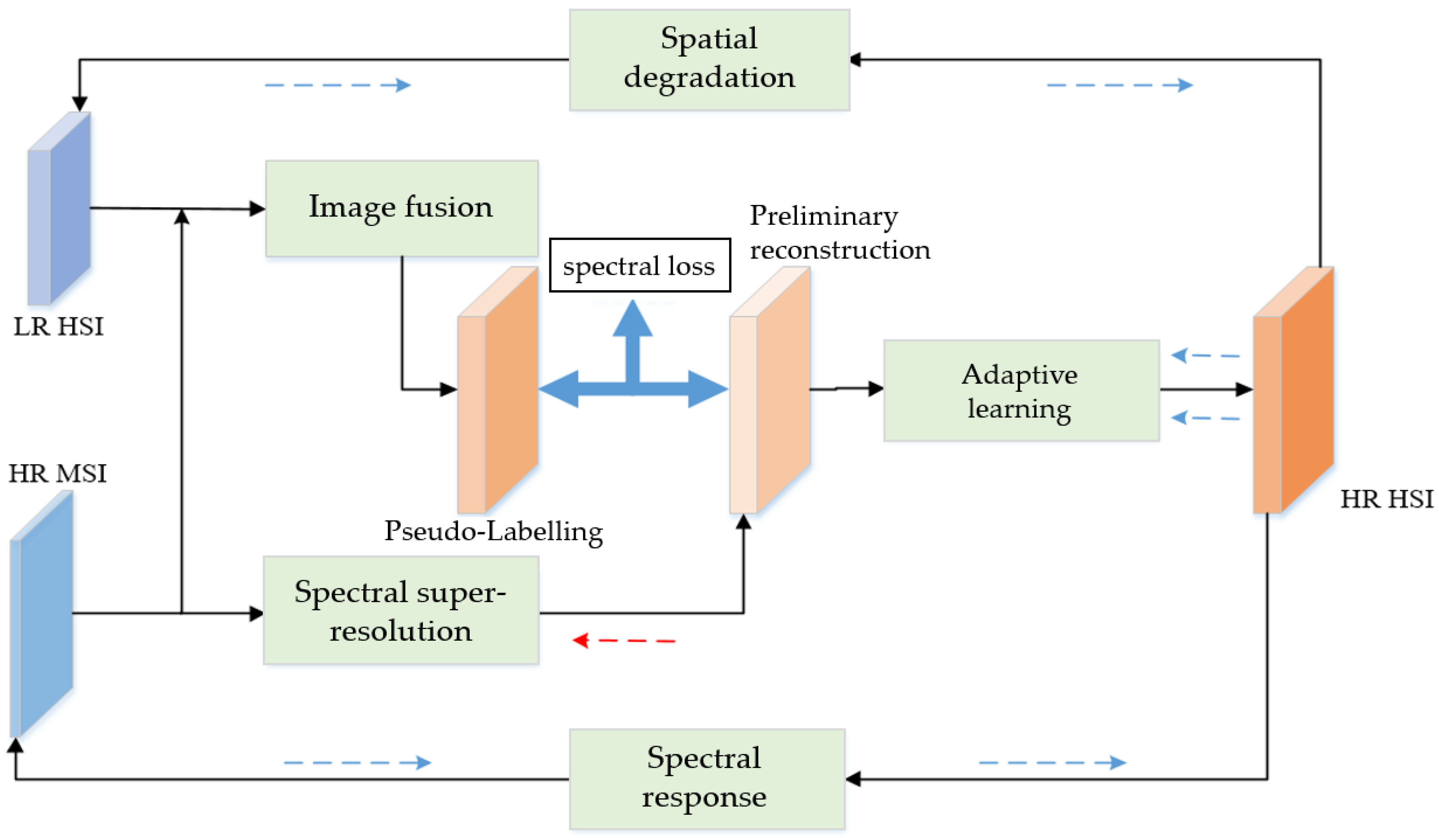
• An adaptive learning-based mapping model is proposed for precise reconstruction and fine classification of HSIs. We innovatively design an adaptive learning module and a self-attention block and felicitously combine them with the image fusion and spectral resolution module, with the aim of enhancing model generalization capabilities and significantly achieving high quality and reconstruction precision.
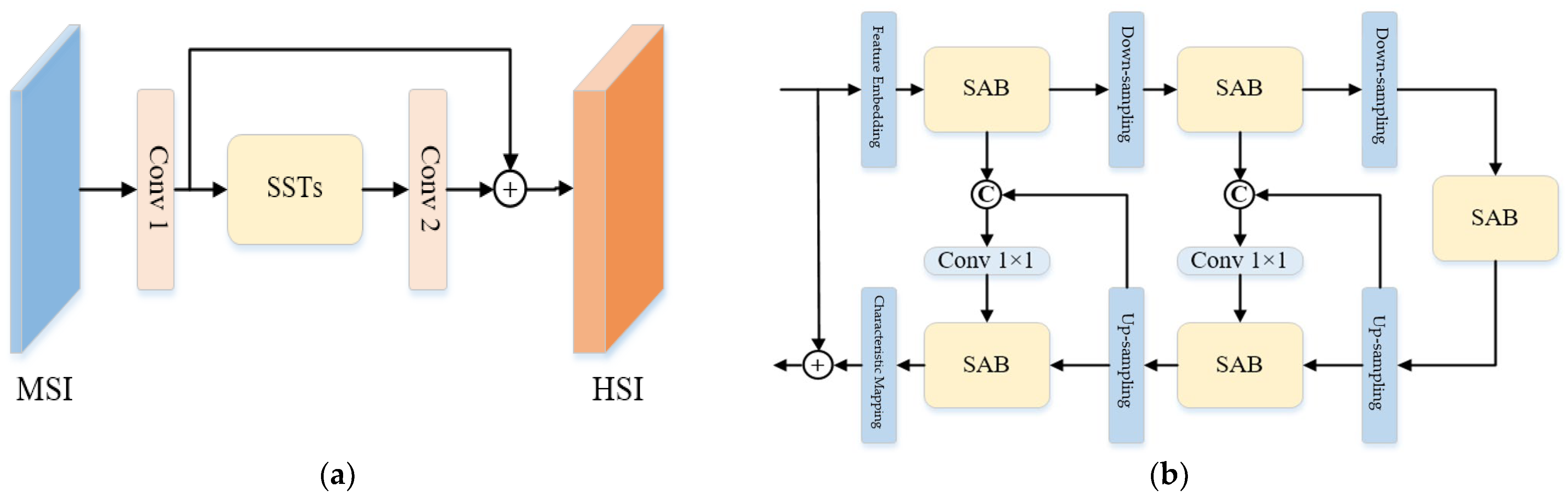
• A self-attention block is innovatively constructed in a spectral super-resolution network to allow the network’s attention to focus on the parts related to the current task, thereby capturing non-local self-similarity and spectral correlation. Moreover, we innovatively design a self-learning network into image reconstruction so as to increase the a priori spectral response function and learn the unknown spatial degradation function. And thus adjust the network structure and parameters dynamically and improve the performance of the model in processing spectral super-resolution tasks.

The remainder of the paper is divided into the following five parts: Section 2 describes the various spectral super-resolution methods published recently based on dictionary learning and deep learning. Section 3 introduces the proposed method in the article. The datasets and the evaluation indicators are mentioned in Section 4. And the experimental results and analysis are described in Section 5. Section 6 presents the conclusion of the work.

2. Related Works

In general, the main challenge of spectral super-resolution is its severe unsuitability, as there can be an infinite amount of hyperspectral data that can be mapped to the same input image under certain constraints. The related studies usually employ the introduction of inherent a priori methods to hyperspectral images to solve the problem mentioned above.

2.1. Spectral Super-Resolution Based on Dictionary Learning

Dictionary learning methods mainly rely on manually setting priors to standardize reconstruction, which depict the structure of hyperspectral images. Arad et al. [14] proposed a spectral super-resolution model based on sparse representation, which pre-learns spectral dictionaries and estimates sparse coefficients by using RGB and hyperspectral training data and a given high spatial resolution RGB image to obtain high-resolution hyperspectral images. In addition, Aeschbacher et al. [15] proposed an improved method by introducing a new shallow learning method to achieve a better spectral super-resolution. In reference [16], sparse representation is used to recover large-scale hyperspectral images from partially overlapping hyperspectral and multispectral images. The sparse representation coefficients and dictionaries are estimated on large-scale multispectral data, and then directly applied to the reconstruction of hyperspectral data.

Fotiadou et al. [17] proposed a coupled dictionary learning model that considers a joint feature space composed of low-spectral resolution and high-spectral resolution hypercubes. By using a framework of sparse representation and dictionary learning, the spectral dimension of the input image is improved to complete the spectral super-resolution. Gao et al. [18] adopted a joint sparse low-rank learning approach to more accurately reconstruct hyperspectral images by jointly learning low-rank multispectral and hyperspectral dictionaries and their corresponding consistent sparse representations. In addition, Han et al. [19] introduced a spectral library to improve the quality of spectral super-resolution based on the joint utilization of multi-hyperspectral images through dictionary learning. Liu et al. [20] proposed a class-guided coupled dictionary-learning method that utilizes the labels of training samples to construct discriminative sparse representation coefficient errors and classification errors as regularization terms, so as to effectively construct the compact and discriminative coupled dictionaries for HSI reconstruction. Liu et al. [21] proposed a method that uses the labels of training samples to construct both class-specific coupled dictionaries and mutually coupled dictionaries, in order to focus on the class-specificity characteristics instead of mutuality characteristics, which is beneficial to classification.

In conclusion, dictionary learning-based methods canonically reconstruct the data by introducing an inherent image prior, whereas it is necessary to set the relevant parameters manually in dictionary learning, and the changes of parameters often have a significant impact on the experimental results. And due to its complex iterative approach, dictionary learning often requires a long time.

2.2. Spectral Super-Resolution Based on Deep Learning

The spectral super-resolution methods based on deep learning rely on the mapping relationship between LR-HSIs and HR-MSIs by constructing a suitable deep network. In these methods, three-dimensional multispectral data are often used as input, and the network reconstructs hyperspectral images by extracting spatial and spectral features from the data. Yan et al. [22] proposed a multi-scale deep convolutional neural network that symmetrically down-samples and up-samples intermediate feature maps through a cascaded paradigm, enabling joint encoding of local and non-local image information for spectral reconstruction. Han et al. [23] proposed a cluster-based multi-branch neural network for end-to-end learning. In addition to spectral similarity, an improved super-pixel segmentation is also introduced to jointly consider spatial contextual information. Hu et al. [24] proposed a high-resolution learning network for hyperspectral data reconstruction, which utilizes a spatial–spectral attention module in high-resolution space to extract pixel-level features and introduces frequency domain learning to reduce frequency domain differences. Similarly, Li et al. [25] also considered feature extraction of channels or frequency bands and proposed a hybrid attention network with structural information consistency, combining spectral gradient constraint loss with mean absolute error as a new loss function. Zamir et al. [26] designed a multi-stage architecture and achieved information exchange between different stages through horizontal and vertical connections.

Moreover, DRCRNet [27] is used to remove the contamination of images by noise, shadows, and other factors. And a dual-channel recalibration module is embedded to adaptively recalibrate channel feature responses, thereby achieving high-fidelity spectrum restoration. The DsTer network [28] combines Transformer and ResNet networks, considering the learning of remote interaction information in images, and finally achieves spectral super-resolution of multispectral remote sensing images. Li et al. [29] proposed a multi-sensor SR framework (MSSRF) based on a two-step approach in which the problems of amplitude inconsistency and band information extraction are solved using an ideal projection network and an ideal multi-sensor SR network, respectively. And Li and Gu et al. introduced a progressive spatial–spectral joint network (PSJN) composed of a 2-D spatial feature extraction module, a 3-D progressive spatial–spectral feature construction module, and a spectral postprocessing module [30].

In addition, a multitemporal spectral reconstruction network (MTSRN) [31] is proposed to reconstruct HS images from multitemporal MS images, which contains a reconstruction network and a temporal features extraction, and a multitemporal fusion network that can independently reconstruct the MS data of a single-phase into HS data and can improve the reconstruction effect by combining neighboring phase information, respectively. Du et al. [32] proposed a novel convolution and transformer joint network (CTJN) including cascaded shallow-feature extraction modules (SFEMs) and deep-feature extraction modules (DFEMs), which can explore local spatial features and global spectral features.

2.3. Attention Mechanism

The attention mechanism originated from the phenomenon that humans can naturally and effectively find salient areas in complex scenes. More specifically, the human visual system filters out less important ones as it processes information, and the system only focuses on the information of interest. The information processing mechanism mentioned above is called the attention mechanism.

The attention mechanism in the network can be seen as a process of dynamically adjusting the weights of input image features based on the task, allowing the network’s attention to focus on key parts of the data, thereby the model can pay more attention to the parts related to the current task and can process the input data more accurately. And ultimately, better results are obtained. From this perspective, traditional neural networks use convolutional operations to feature map the input image, allowing the network to focus on features that are more closely related to the task. The process above is also a simple attention mechanism.

The characteristics of the attention mechanism can be expressed as:

$$Attention=f(g(x),x)$$

(1)

in which $g(x)$ represents the process of the network paying attention to key areas by entering information. And $f(g(x),x)$ represents the procedure of processing input data based on $g(x)$. Particularly, for the self-attention mechanism, the specific process in the Formula (1) can be expressed as:

$$Q,K,V=Linear(x)$$

(2)

$$g(x)=Softmax(QK)$$

(3)

$$f(g(x),x)=g(x)V$$

(4)

According to the different domains that the attention module focuses on, attention mechanisms can be divided into channel attention, spatial attention, temporal attention, self-attention, mixed attention, etc.

The channel attention mechanism is able to automatically learn the weights of each channel based on the task. Apparently, in neural networks, different channels often represent different image features. Therefore, the process of channel attention can be seen as a feature selection process that enables the network to focus on key features.

The core of the basic channel attention mechanism is a compression–excitation module, which learns the relationships between different channels by using global average pooling layers, fully connected layers, and nonlinear layers. And, ultimately, output attention vectors. Accordingly, the corresponding elements are multiplied in the vectors to change the input features of each channel. In this case, if $X$ is used as the input and $Y$ is used as the output, the process can be expressed as follows:

$$g(x)=\sigma (W_2\delta (W_{1}GAP(X)))$$

(5)

$$Y=g(x)X$$

(6)

where $W_1$ and $W_2$ represent the fully connected layers, and $GAP(·)$ represents the function of global pooling. Moreover, $\delta$ and $\sigma$ represent the activation functions $ReLU(·)$ and $Sigmoid(·)$, respectively. The channel attention module not only suppresses noise but, in particular, emphasizes the important characteristic channels. Moreover, it requires lower computational resources. Accordingly, a channel attention module can be added after each residual unit.

The spatial attention mechanism is an adaptive region selection mechanism based on targets, which focuses attention on the target region while suppressing feature activation in irrelevant regions. In reality, the attention gate is a representative spatial attention module, in which, given the input feature map $X$, the process can be represented as:

$$g(x)=\sigma (\phi (\delta ({\varphi }_x(X)+{\varphi }_g(G))))$$

(7)

$$Y=g(x)X$$

(8)

where $G\in {ℝ}^{C\times H\times W}$ represents the gating signal, which is collected at a coarser scale. We can use additive attention to obtain the gating coefficients. Particularly, the gating signal provides activation and contextual information for image regions, and the spatial regions of interest are selected by analyzing this signal. Then, $\phi (·)$, ${\varphi }_x(·)$, ${\varphi }_g(·)$ represent 1 × 1 convolution operation. Similarly, $\delta$ and $\sigma$ represent the activation functions named $ReLU(·)$ and $Sigmoid(·)$, respectively. Furthermore, $Y$ represents the output of the module. Undeniably, attention gates guide the model’s attention to the desired spatial regions while suppressing feature activation in irrelevant regions. Due to the lightweight design, the representational capacity of the model is greatly enhanced without significantly increasing computational costs. Moreover, the model is universal and modular, which makes it easy to use in various neural network models.

The temporal attention mechanism is an adaptive mechanism for dynamically selecting temporal regions, which determines the time periods requiring attention, and the mechanism is commonly used for video processing. In fact, the time-adaptive module efficiently and flexibly captures complex time relationships in low complexity. And the module mainly includes two branches: the localized branch and the global branch, respectively. Let $X\in {ℝ}^{C\times T\times H\times W}$ represent the input feature, which contains the time dimension, and thus the localized branch can be expressed as:

$$g(x)=\sigma (Conv1D(\delta (Conv1D(GAP(X)))))$$

(9)

$$X_1=g(x)X$$

(10)

The global features focus on generating a channel-based adaptive kernel, which relies on the global temporal information of each channel. And for the $C-th$ channel, the kernel can be written as:

$${\mathrm{\Theta }}_c=Softmax(F{C}_2(\delta (F{C}_1(GAP{(X)}_c))))$$

(11)

where $FC(·)$ represents the fully connected layer, and $Conv1D(·)$ represents the convolution operation of 1D. The final output of the module can be expressed as:

$$Y=\mathrm{\Theta }\otimes X_1$$

(12)

3. Proposed Method

3.1. Network Structure

The overall structure of the proposed method is shown in Figure 1. Both low-resolution hyperspectral images (LR-HSI) and high-resolution multispectral images (HR-MSI) covering the same area were required as training data for the network. The network was trained unsupervised to reconstruct high-spatial-resolution hyperspectral images for large scenes (HR-HSI) with the LR-HSI and the HR-MSI reference images. Thus, completing the collaborative mapping of the original hyperspectral image at the spatial scale.

Firstly, multispectral and hyperspectral images were used as inputs, and the image fusion module was used in the network to generate pseudo labels. Secondly, the spectral super-resolution network was supervised and trained based on the pseudo labels to learn the general image prior information of the mapping from MSIs to HSIs. Then, the output of the spectral super-resolution network was used to calculate the loss with the pseudo labels generated by the fusion module and, thus, guide the update of network parameters. As shown in Figure 1, the red dashed line represents the direction of gradient backpropagation in the spectral super-resolution network.

Then, an adaptive learning module was designed for the preliminary reconstructed images generated by the spectral super-resolution network, with the aim of learning the residuals between the preliminary reconstructed images and the real HSI to correct the influence of pseudo labels on the reconstruction results. Finally, the output of the adaptive learning module was HR-HSIs. They were reconstructed from the original input data of LR-HSIs and HR-MSIs using a special degradation network and a given spectral response function. And then the loss was calculated to guide the spatial degradation process of the network learning image and update the parameters of the adaptive learning module. As shown in Figure 1, the blue dashed line represents the direction of gradient backpropagation in the adaptive learning network. It should be noted that the image fusion module in the model requires the GLP fusion scheme [33], which completes image fusion in an unsupervised manner.

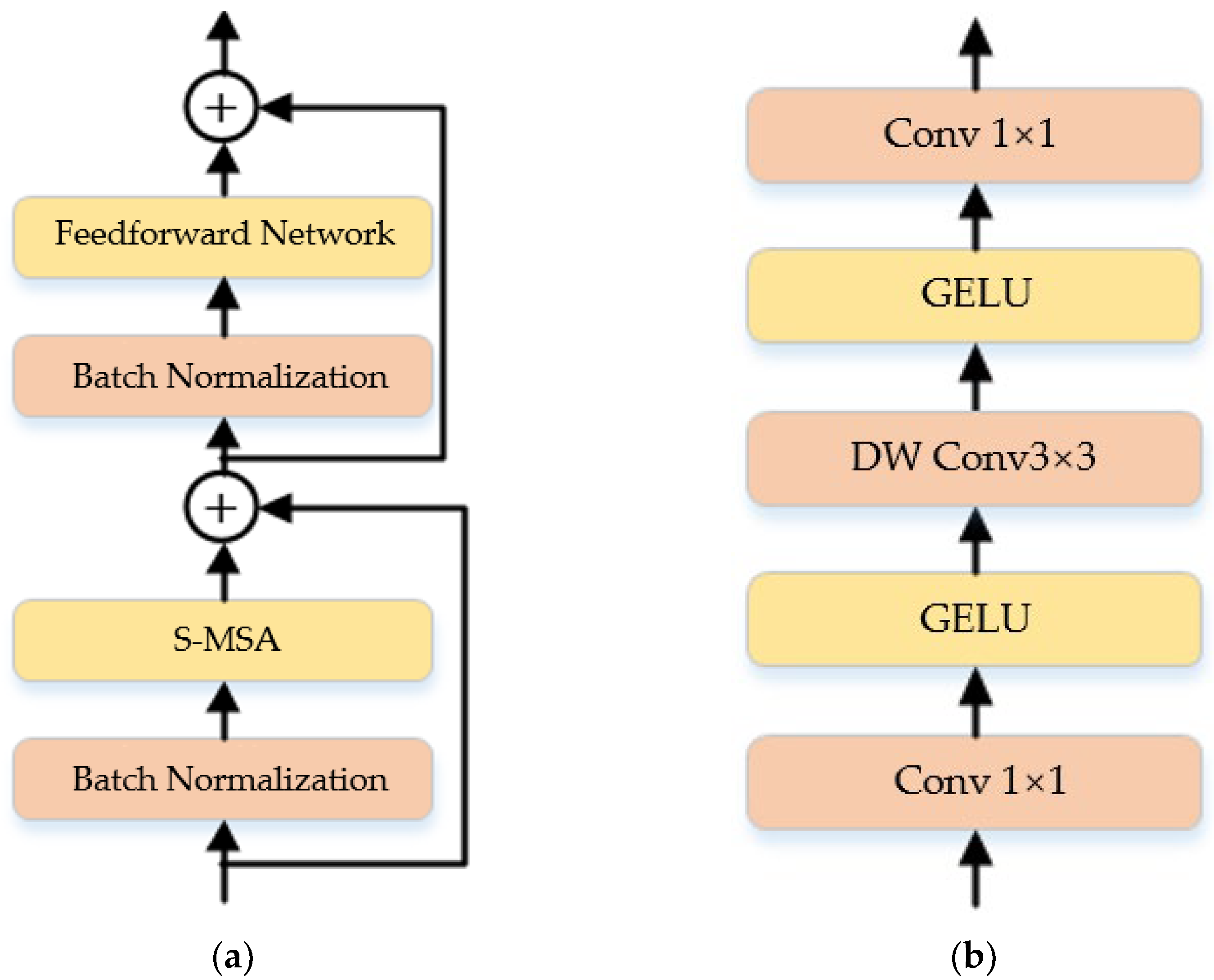
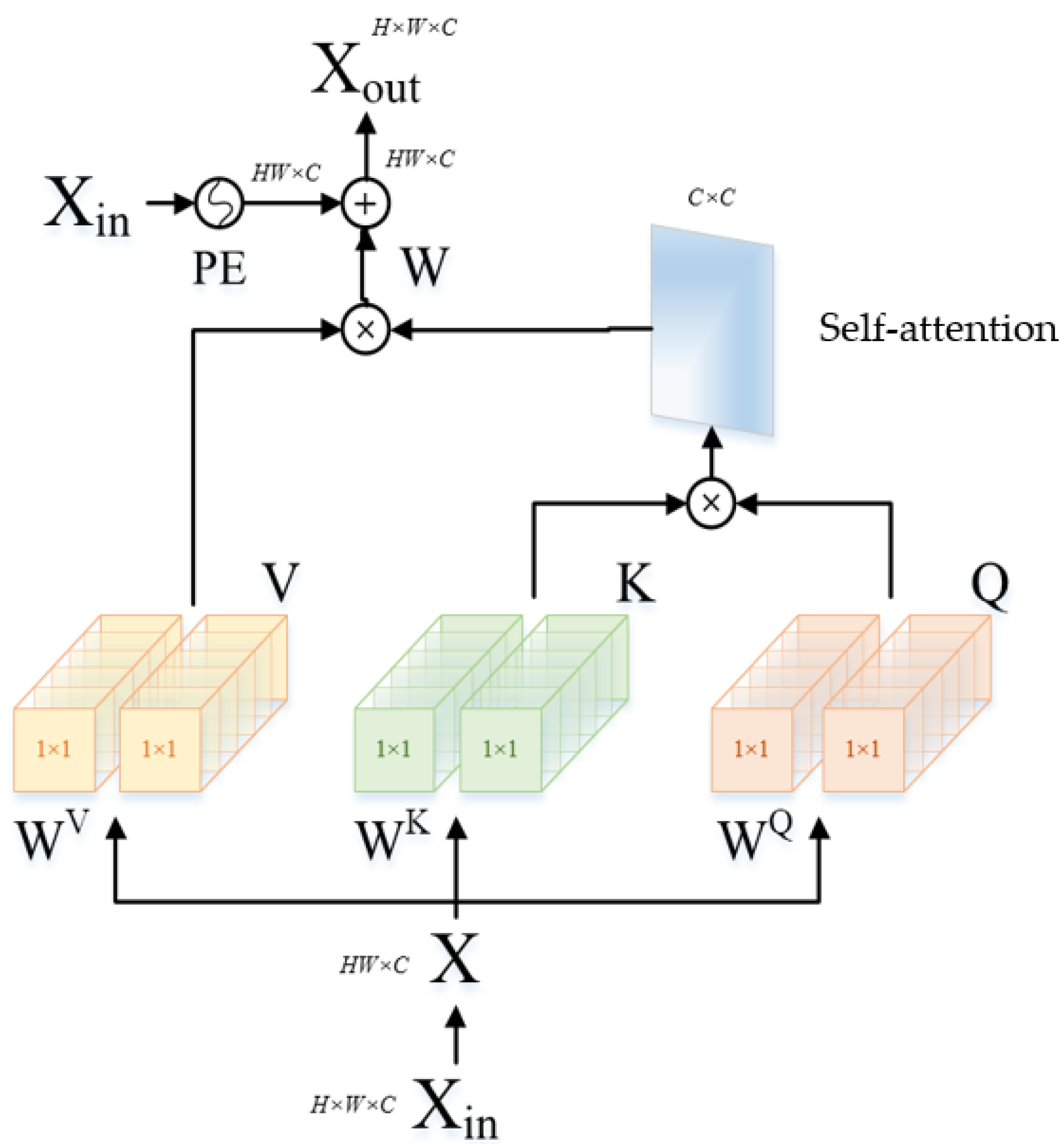
3.2. Spectral Super-Resolution Network Based on Self-Attention Mechanism

The attention mechanism in the network can be seen as a process of dynamically adjusting the weights of input image features based on the task, allowing the network’s attention to focus on key parts of the data, thereby the model can pay more attention to the parts related to the current task and can process the input data more accurately. And ultimately, better results can be obtained. For the task of spectral super-resolution, compared to traditional convolutional neural networks, the self-attention-based model has certain advantages in capturing non-local self-similarity and remote correlation. The structure of the spectral super-resolution model adopted in Figure 1 is shown in Figure 2.

Firstly, the network performs a feature mapping against the input MSI, where the mapping part of Conv1 includes two progressive 3 × 3 convolution operations, which can raise the dimensions of the feature. Furthermore, the mapping part of Conv2 contains a 3 × 3 convolution operation that keeps the feature dimension unchanged. Particularly, the network has residual connections between the output of Conv1 and Conv2.

The main part of the network is composed of multiple cascaded single-stage spectral transformation modules (SST). And the structure of SST is shown in Figure 2b. Specifically, the main part of the module is symmetrically connected as a U-shaped structure. And three blocks are included in SST: the up-sampling block, the down-sampling block, and the spectral attention block (SAB), ensuring that the network can generate features of different levels. At the same time, jump connections between the corresponding levels of the encoder and the decoder are designed to accomplish feature aggregation, where the feature embedding and the feature mapping modules are both composed of 3 × 3 convolutional operations with constant input and output feature dimensions. Moreover, the down-sampling block is a stepwise 4 × 4 convolution, which increases the number of channels in the feature map while decreasing the size of the feature map. Furthermore, the up-sampling block is a stepwise 2 × 2 transposed convolution. With the aim of avoiding information loss during up-sampling, a hopping connection is maintained between the decoder and the encoder while undergoing a 1 × 1 convolution block for feature aggregation. Ultimately, the residual connection is established between the output and the input of the module.

The specific structure of the spectral attention module (SAB) is shown in Figure 3, which is mainly composed of three kinds of blocks for serial connections: the batch normalization, the feed-forward network, and the spectral multi-headed self-attention module (S-MSA), with residual connections between the inputs and outputs of the module. Moreover, the batch normalization makes the forward propagation of the network more stable, and at the same time makes the process of gradient backpropagation more stable, which avoids the overfitting of the network to some degree. And, as shown in Figure 3b, the feed-forward network consists of three blocks serially connected: the 1 × 1 convolution, the 3 × 3 depth-wise convolution, and the GELU activation function.

Specifically, the structure of the spectral multi-headed self-attention module (S-MSA) is shown in Figure 4. The module considers each spectral feature map as a unit and calculates the autocorrelation along the spectral dimension to capture non-local correlations.

In the S-MSA, firstly, recombine the input feature maps $X_{in}\in {ℝ}^{H\times W\times C}$ as $X\in {ℝ}^{HW\times C}$, and thus perform three linear feature maps to obtain $Q$, $K$ and $V$, respectively.

$$Q=X{W}^Q,K=X{W}^K,V=X{W}^V$$

(13)

where $Q$, $K$, and $V$ are the learnable parameters. Then, the three features are divided into heads along the spectral channel dimension: $Q=\left[Q,\cdots ,Q_N\right]$, $K=\left[K,\cdots ,K_N\right]$ and $V=\left[V,\cdots ,V_N\right]$. And the size of each head is $d_h=C/N$. As shown in Figure 4, we have $N=1$ at this point. And then, self-attention is calculated according to the obtained $Q,K$ and Formula (14):

$$A_j=softmax({\sigma }_j{K}_j^T{Q}_j),head=V_j{A}_j$$

(14)

where $K_j^T$ represents the transpose of the matrix $K^T$. ${\sigma }_j$ is a learnable parameter. In the network, $K_j^T{Q}_j$ is re-weighted by ${\sigma }_j$ to accommodate the self-attention named $A_j$. And then, the output features of divided heads are aggregated and undergo linear mapping. Finally, the positional information about the spectral features is embedded, and we can obtain the final output of the module $X_{out}\in {ℝ}^{H\times W\times C}$.

$$X_{out}=\left(\underset{j=1}{\overset{N}{concat}}(hea{d}_j)\right)W+f_p(V)$$

(15)

where $W\in {ℝ}^{C\times C}$ is a learnable parameter and $f_p(·)$ is a function that generates position information, which includes two 3 × 3 depth-wise convolutions, a GELU nonlinear activation function, and the recombination process. In reality, the purpose is to ensure that the position information of different spectral units can be saved in advance when the module operates on the input through the network.

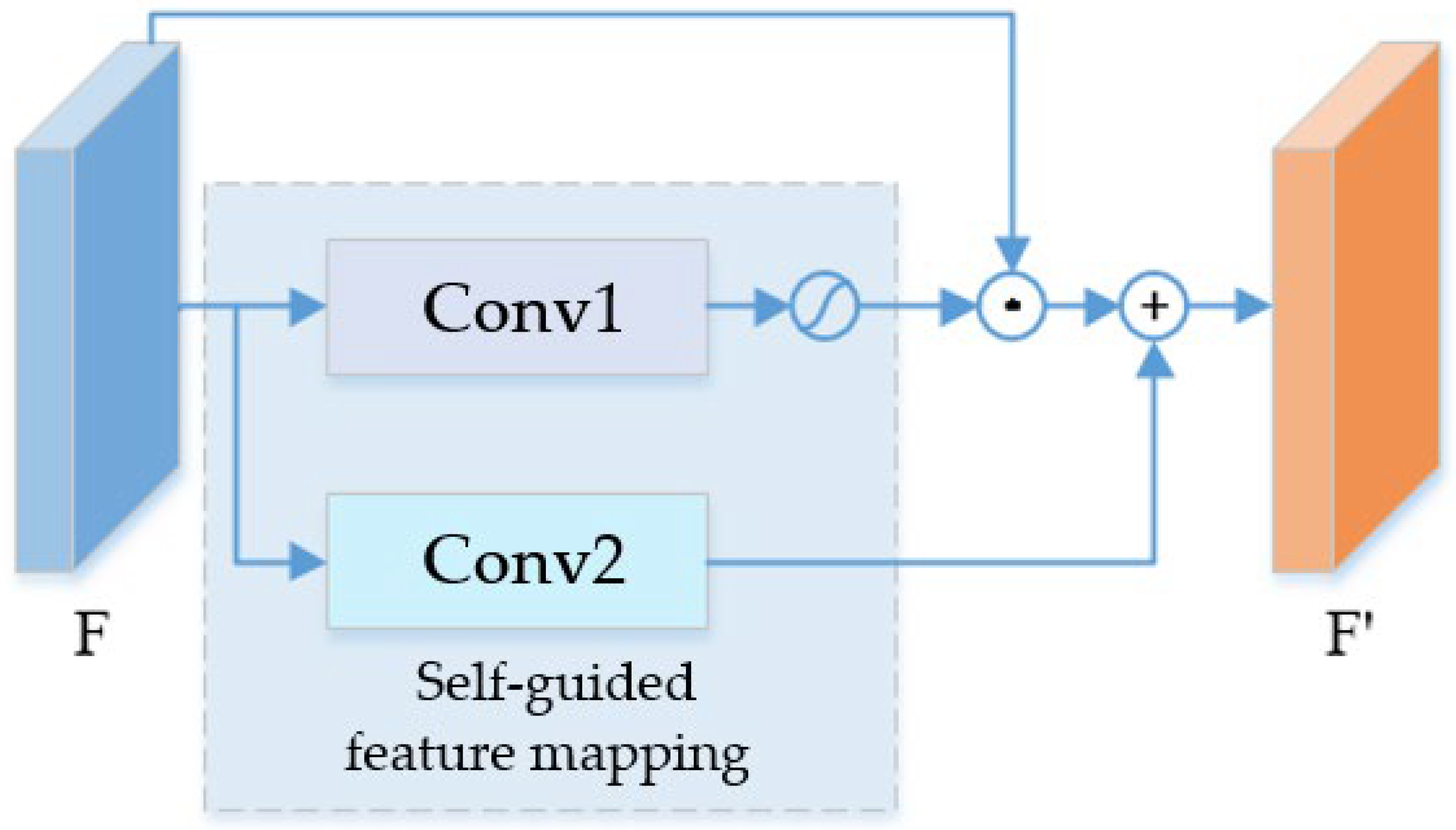
3.3. Adaptive Learning Network

Based on the pseudo labels obtained by the fused multispectral and hyperspectral training data, the spectral super-resolution network can generate preliminary reconstructed images with high spatial spectral resolution. Specifically, in order to introduce the spectral response function priors into the model and learn the specific spatial degradation function of the image, an adaptive learning module is required in the network for the preliminary reconstructed images. Through the spatial degradation network and the given spectral response function, the preliminary reconstructed image is mapped to the original HSI and MSI, respectively, as shown in Figure 3, by adjusting the residual pixel by pixel and refining the specific details of the image to complete unsupervised adaptive learning.

The training process of the adaptive learning module can be represented by Formula (16):

$$\underset{\theta ,\vartheta }{\min }{‖Y_m-RZ‖}^2+{‖Y_m-ZH‖}^2, s.t. Z=\mathcal{G}\left(Z^{\prime };\theta \right),ZH=\mathcal{H}\left(Z^{\prime };\vartheta \right)$$

(16)

where $Z^{\prime }$ is the preliminary reconstructed images generated for the spectral super-resolution network, and $Z$ represents a reconstructed image of the final output in the network. Moreover, $\mathcal{G}\left(Z^{\prime };\theta \right)$ represents the feature mapping process of adaptive learning modules, and $\mathcal{H}\left(·;\vartheta \right)$ represents the process of image space degradation. And specifically, $\theta$ and $\vartheta$ are the learnable parameters in the adaptive learning module and the spatial degradation networks, respectively.

The main structure of the adaptive learning network is shown in Figure 5. In order to recover specific details of the image, a residual architecture is introduced in the module, which mainly includes a feature mapping block, self-guided block, and output convolutional layer. For the input image $Z^{\prime }$, firstly, the module performs three layers of 3 × 3 convolution operations, which keeps the input and output feature dimensions invariant and performs the ReLU activation function. This is followed by self-guided modules and single-layer convolution operations, so as to ensure that the main part of the module can recover the residual between the real HS image and the initially reconstructed image of the spectral super-resolution network. Then, eventually, the output image, named $Z$, is obtained by making a residual connection with the input image.

The structure of the self-guided module in the network is shown in Figure 6. Specifically, the input feature guides the output feature of the network through two branches, assuming that $F$ and $F^{\prime }$ are the input and output features of the self-guided module, respectively. Therefore, the feature mapping process of the module can be represented as follows:

$$A=P_1(F;{\upsilon }_1);B=P_2(F;{\upsilon }_2)$$

(17)

$$F^{\prime }=A·F+B$$

(18)

where $P_1(·)$ represents the process of convolution Conv1 and the activation function $Sigmoid(·)$, and then $P_2(·)$ represents the operation of convolution named Conv2. Moreover, $A$ and $B$ are the output of the middle layer.

For the spatial degradation network in the adaptive learning process, and considering the limited amount of data in the MSI and HSI, the structure of the network should be designed to minimize the computational complexity in the unsupervised learning process in order to avoid the overfitting of the network. Therefore, the model adopts a simple structure to implement the degradation network to greatly reduce the number of parameters in the learning process. In reality, it often involves spatial down-sampling, spatial blurring, and noise destruction in the image spatial degradation process, where the process of spatial down-sampling and spatial blurring can be expressed as the convolution of the image and a specific kernel, and, specifically, the impact of the noise is close to the addictive zero-mean stochastic noise. Therefore, the process of spatial degradation can be expressed as:

$$ZH=(Z\ast k){\downarrow }_s+N$$

(19)

where $k$ represents a two-dimensional spatial convolution kernel, and $\ast$ represents the convolution of the same kernel $k$ and each band of the image, respectively. $S$ represents the scaling factor for spatial down-sampling, and $N$ represents the additive noise. In order to design the structure of the network, a single two-dimensional convolutional layer with a step size $S$ is used to achieve spatial down-sampling and blur. Particularly, the main learnable parameter is the convolutional kernel named $k$. And seeing that the loss function designed in Formula (16) has the function of absorbing additive noise, there is no need to design a specific structure for $N$.

4. Experimental Datasets and Evaluation Indicators

4.1. Experimental Datasets

The hyperspectral data involved in the experiment are the Houston data and the GF-YR data, where the Houston data were released by the IEEE GRSS Data Fusion Contest (DFC) in 2013, which was acquired at the Houston University campus and nearby area. The LR-HSI and the HR-MSI were obtained from spatial and spectral down-sampling of the raw Houston data, respectively. Furthermore, we obtained the GF-5 hyperspectral and labeling data from the First Marine Institute, Department of Natural Resources, which were acquired over the Yellow River Delta National Nature Reserve in China.

Table 1. Experimental datasets.

Dataset	HSI or MSI	Source	Image Size	Number of Bands	Spatial Resolution
Houston	HSI	CASI	171 × 951	144	5 m
	MSI	simulate	342 × 1902	4	2.5 m
GF-YR	HSI	GF5	734 × 763	295	30 m
	MSI	GF1	1468 × 1526	4	15 m

lists the image size, source, spatial resolution, band number, and other indicators of the experimental data.

(1)

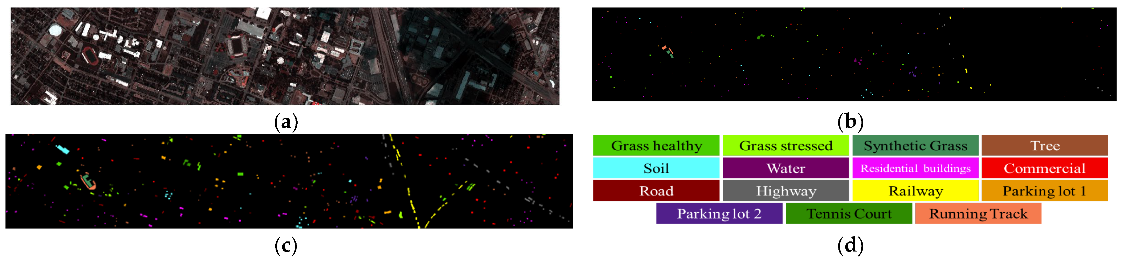
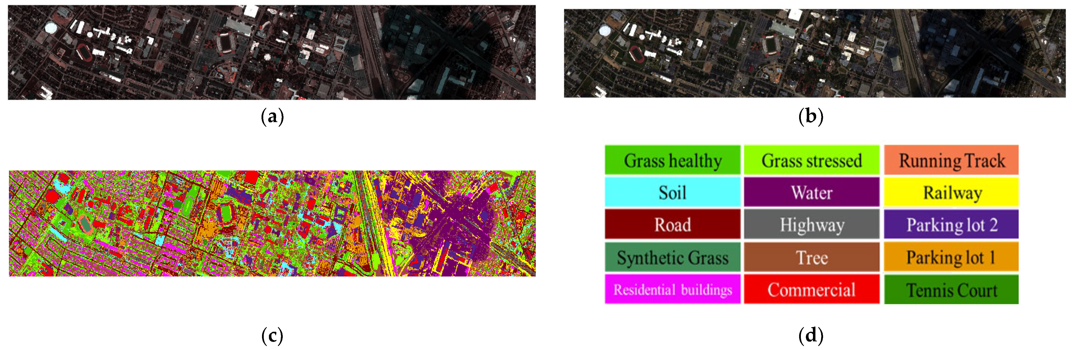
The Houston data were acquired by the ITRES CASI-1500 sensor (ITRES, Calgary, AB, Canada). The raw image data size is 349 × 1905, and the data have a total of 144 bands, covering the spectral range of 364–1046 nm. As shown in Figure 7, 71, 39, and 16 bands are selected for false-color display. Moreover, Figure 7b,c show the training set and test set labels. And the number of labels for class training sets and test sets during the classification of Houston data is listed in

Table 2. Houston labeling data.

Labels	Categories	Number of Training Labels	Number of Testing Labels
1	Grass healthy	537	699
2	Grass stressed	61	1154
3	Synthetic Grass	340	357
4	Tree	209	1035
5	Soil	74	1168
6	Water	22	303
7	Residential buildings	52	1203
8	Commercial	320	924
9	Road	76	1149
10	Highway	279	948
11	Railway	33	1185
12	Parking lot 1	329	904
13	Parking lot 2	20	449
14	Tennis Court	665	162
15	Running Track	279	381

.

(2)

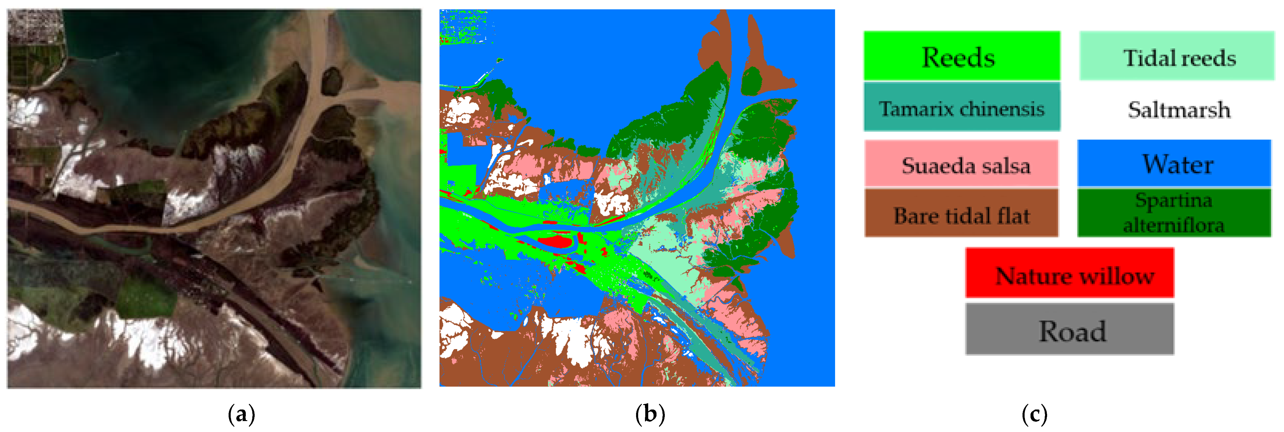
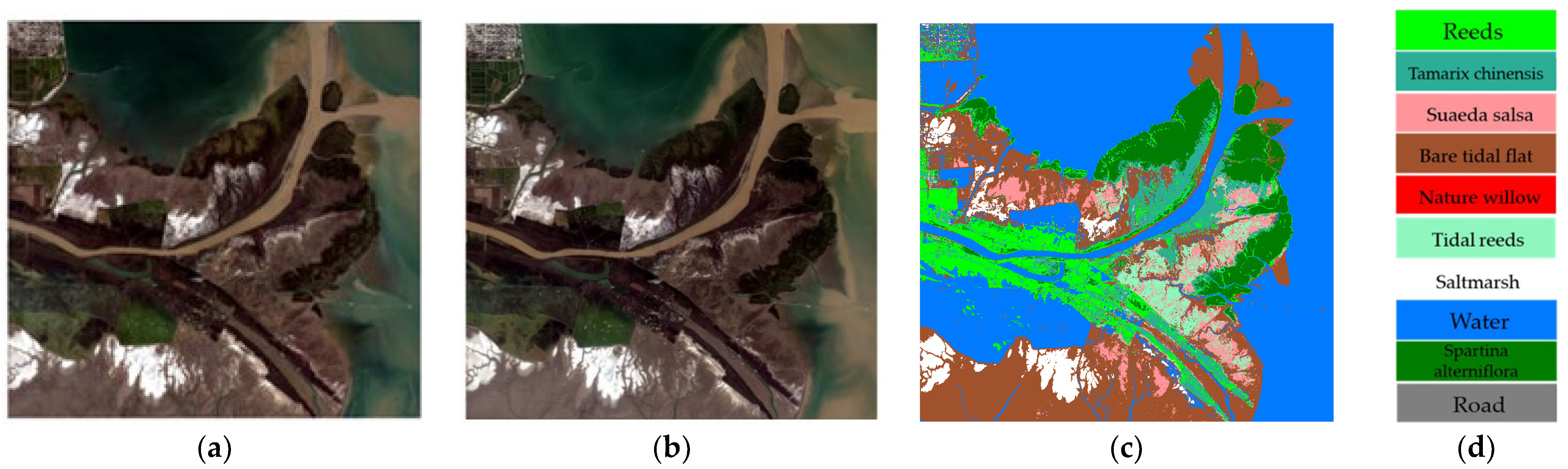
The hyperspectral and multispectral data of GF-YR were acquired by the Gaofen-5 and Gaofen-1 satellites, respectively. The multispectral camera on the Gaofen-1 satellite (GF-1) can provide multispectral data. The data have four different bands, with the range of 450–520 nm, 520–590 nm, 630–690 nm, and 770–890 nm, respectively. Moreover, the Gaofen-5 satellite (GF-5) has the highest spectral resolution among the national Gaofen major projects. It was officially launched in 2019 with six payloads, including a full-band spectral imager with a spatial resolution of 30 m. Moreover, the imaging spectrum covers 400~2500 nm, including a total of 330 bands, and the visible spectral resolution is 5 nm. In reality, it has retained 295 bands after removing bad bands by preprocessing the satellite data. Figure 8 shows the image of GF-5, and 56, 39, and 25 bands are selected for false-color display of the HSI image. Figure 8c introduces a schematic representation of the category labels, which lists the features corresponding to each color. Furthermore,

Table 3. GF-YR labeling data.

Labels	Categories	Number of Global Labels
1	Reeds	171,779
2	Tamarix chinensis	104,809
3	Tidal reeds	83,161
4	Saltmarsh	76,206
5	Suaeda salsa	102,579
6	Naked tidal flat	436,015
7	Water	1,066,570
8	Spartina alterniflora	180,186
9	Nature willow	13,492
10	Road	5371

shows the number of various labels of GF-YR data.

4.2. Evaluation Indicators

In the experiment, we evaluated the reconstruction similarity and classification accuracy of the reconstructed images to assess their overall quality and performance.

Firstly, the reconstructed HSIs were evaluated using various indexes, encompassing different perspectives. The article utilizes the following indicators: peak signal-to-noise ratio (PSNR), the spectral angle index (SAM), the structural similarity (SSIM), spectral distortion index ($D_{\lambda }$), spatial distortion index ($D_s$), and the global image quality (QNR). Secondly, we evaluated the classification results of reconstructed HSIs using overall accuracy (OA).

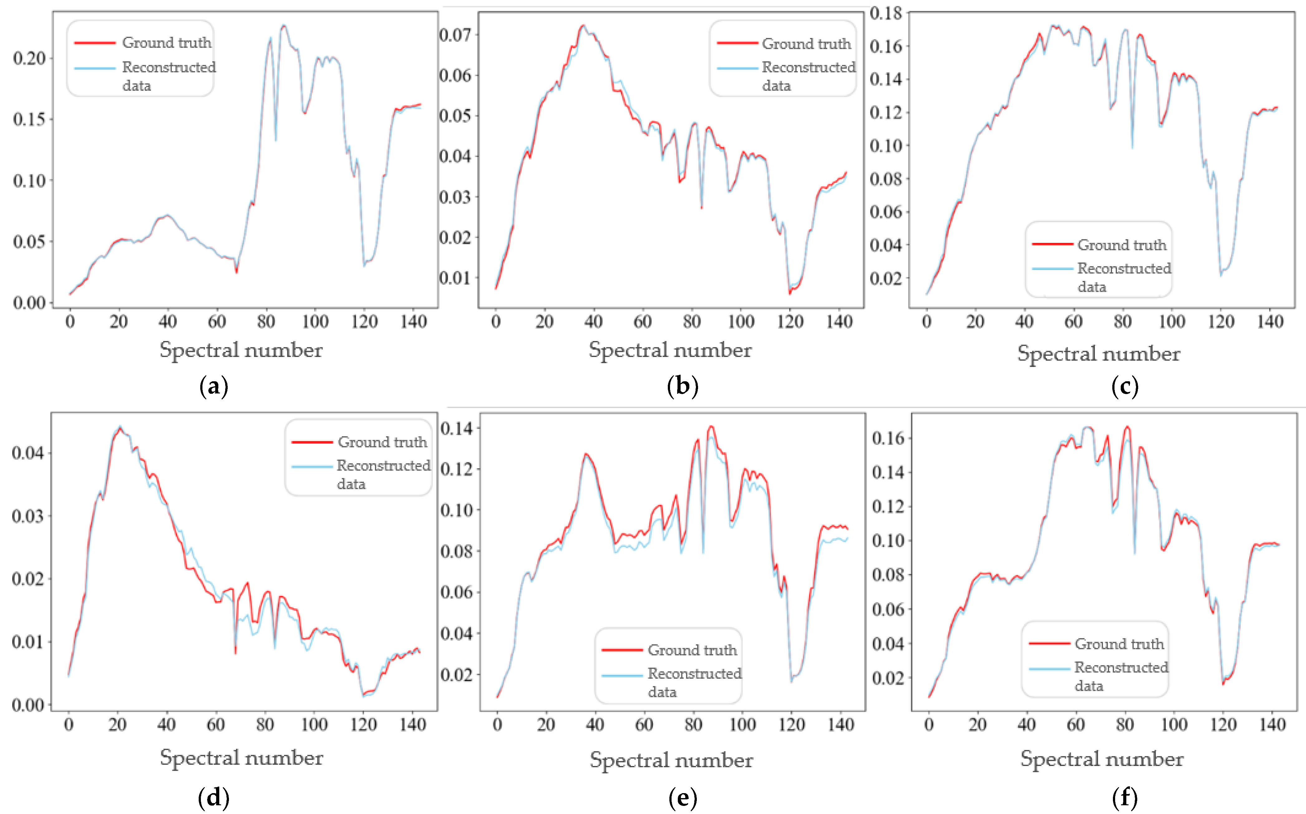
• PSNR was used to measure the distortion after compression. Higher PSNR values indicate smaller image distortion, and indicate a higher image similarity. Generally, a PSNR value above 30 indicates fine image quality.

  $$RMSE=\sqrt{\frac{1}{HWN}{\displaystyle \sum _{l=1}^N{\displaystyle \sum _{i=1}^H{\displaystyle \sum _{j=1}^W{\left(u_l\left(i,j\right)-\widehat{u_l}\left(i,j\right)\right)}^2}}}},PSNR=20\lg \frac{1}{RMSE}$$

  (20)

  where $u$ is a real HSI, $\widehat{u}$ represents the reconstructed HSI. $N$, $H$, and $W$ represent the number of bands, height, and width of the image, respectively.
• SAM determines the spectral similarity by calculating the angle of spectrum vectors between the reconstructed image and the real HS image, so as to quantify the spectral information retention of each pixel. Closer SAM values to zero indicate less spectral distortion, manifesting a higher level of spectral similarity.

  $$SAM=\frac{1}{HW}{\displaystyle \sum _{i=1}^H{\displaystyle \sum _{j=1}^W\arccos \left(\frac{〈u\left(i,j\right),\widehat{u}\left(i,j\right)〉}{\left|u\left(i,j\right)\right|\left|\widehat{u}\left(i,j\right)\right|}\right)}}$$

  (21)

  where $〈·〉$ represents the inner product of the vector, and $\left|·\right|$ represents the module of the vector.
• The similarity of the overall structure between the real HS image and the reconstructed image was evaluated by SSIM. Closer SSIM values to one indicate higher image similarity.

  $$SSIM=\frac{\left(2{\mu }_u{\mu }_{\widehat{u}}+c_1\right)\left(2{\sigma }_u{\sigma }_{\widehat{u}}+c_2\right)}{\left({\mu }_u^2+{\mu }_{\widehat{u}}^2+c_1\right)\left({\sigma }_u^2+{\sigma }_{\widehat{u}}^2+c_2\right)},c_1={(k_{1}L)}^2,c_2={(k_{2}L)}^2,c_3=c_2/2$$

  (22)

  where ${\mu }_u$, ${\mu }_{\widehat{u}}$ represent the mean of $u$ and $\widehat{u}$, respectively. Moreover, ${\sigma }_u^2$, ${\sigma }_{\widehat{u}}^2$ represent the variance of $u$ and $\widehat{u}$, respectively. And $c_1,c_2,c_3$ are constants, avoiding the denominator tending to a zero value to make the calculation more stable. Default $k_1=0.01,k_2=0.03$, $L$ is the range of pixel values in the image.
• $D_{\lambda }$ is used to measure the spectral distortion of the reconstructed image. The closer the value is to zero, the smaller the spectral distortion.

  $$Q({\widehat{u}}_i,{\widehat{u}}_j)=\frac{4{\sigma }_{{\widehat{u}}_i{\widehat{u}}_j}{\overline{\widehat{u}}}_i{\overline{\widehat{u}}}_j}{({\sigma }_{{\widehat{u}}_i}^2+{\sigma }_{{\widehat{u}}_j}^2)({\overline{\widehat{u}}}_i^2+{\overline{\widehat{u}}}_j^2)}$$

  (23)

  $$D_{\lambda }=\sqrt[q]{\frac{1}{N(N-1)}{{\displaystyle \sum _{i=1}^N{\displaystyle \sum _{j=1,j\ne i}^N\left|Q({\widehat{u}}_i,{\widehat{u}}_j)-Q(H_i,H_j)\right|}}}^q}$$

  (24)

  where $\widehat{u}$ represents the reconstructed image, $\overline{\widehat{u}}$ represents the average of pixels in the image $\widehat{u}$. $H$ represents the LR-HSI.
• $D_s$ is used to measure the degree of spatial information loss of the image. Closer $D_s$ to zero leads to less spatial loss of the image.

  $$D_s=\sqrt[q]{\frac{1}{N}{{\displaystyle \sum _{i=1}^N\left|Q({\widehat{u}}_i,M)-Q(H_i,\tilde{M})\right|}}^q}$$

  (25)

  where $M$ is a HR-MSI. And $\tilde{M}$ is a multispectral image after the down-sampling of $M$, which has the same spatial resolution as $H$.
• QNR measures the global quality of the image. If QNR is close to one, the image quality is higher. The calculation method is calculated as follows:

  $$QNR={(1-D_{\lambda })}^{\mu }{(1-D_s)}^{\rho }$$

  (26)

5. Results and Analysis

5.1. Data Preprocessing

The datasets used in the experiment are Houston and GF-YR, which need to be preprocessed before the experiment. And the size of the overlapping area between HSI and MSI in the Houston data is 70 × 1902. During the training process, the data preprocessing was performed as follows. Firstly, crop the overlapping regions to multiple 64 × 64 image blocks, which keeps the 50% repetition rate to ensure the coverage of the entire training area. Then, crop the original training image by randomly selecting a starting point. And finally, keep the number of training blocks to 800. The partially cropped training data are shown in Figure 9.

Furthermore, for GF-YR data, the size of the overlapping area is 500 × 500, and the regions are cropped to multiple 128 × 128 image blocks. Similarly, the GF-YR data also need to keep a 50% repetition rate to ensure the coverage of the training area, and then we also need to randomly select a starting point to choose the training field. And eventually, keep the number of training blocks to 500.

During the image testing process, considering the amount of data in the image and the memory usage during program operation, the original test image also needs to be cropped. Specifically, the Houston data were cropped to 10 image blocks with the size of 336 × 336. This requires certain areas of overlap between different image blocks, which results in a total image size of 336 × 1902. Similarly, the GF-YR data were cropped to 256 × 256 image blocks with a data volume of 64 and, after splicing, the full image size was 1468 × 1562. During the splicing process, the pixel values of the overlapping regions were determined by taking the average.

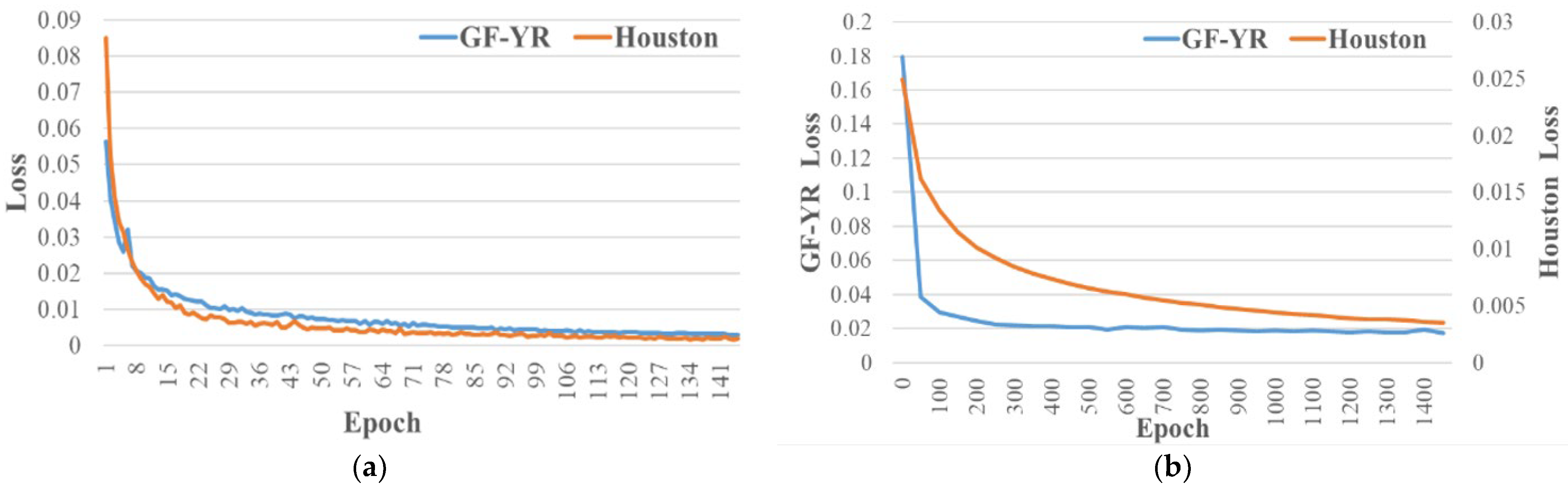
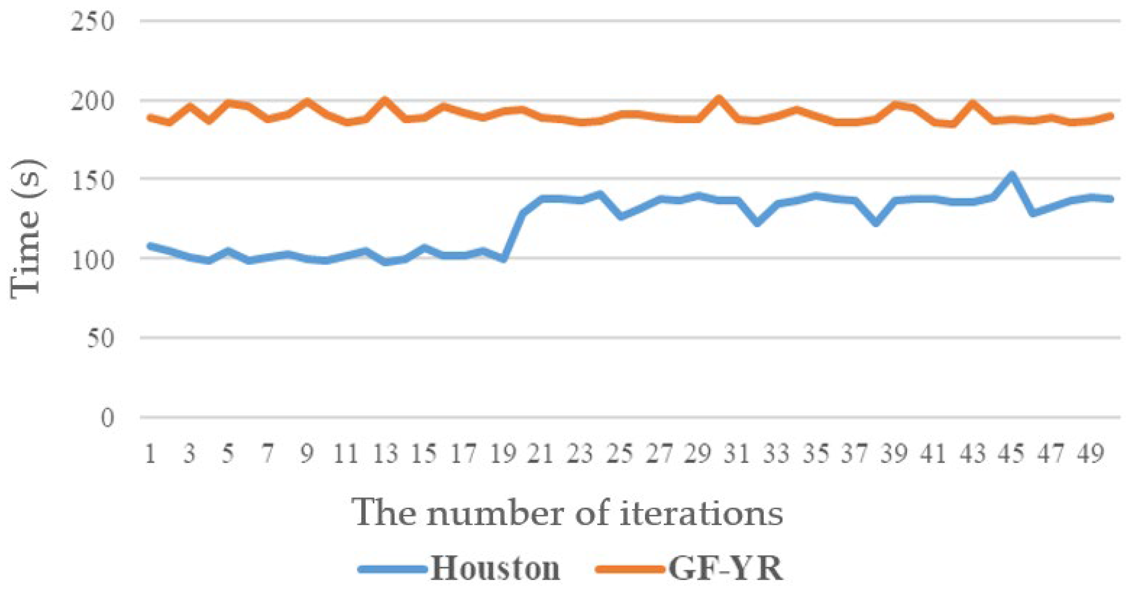
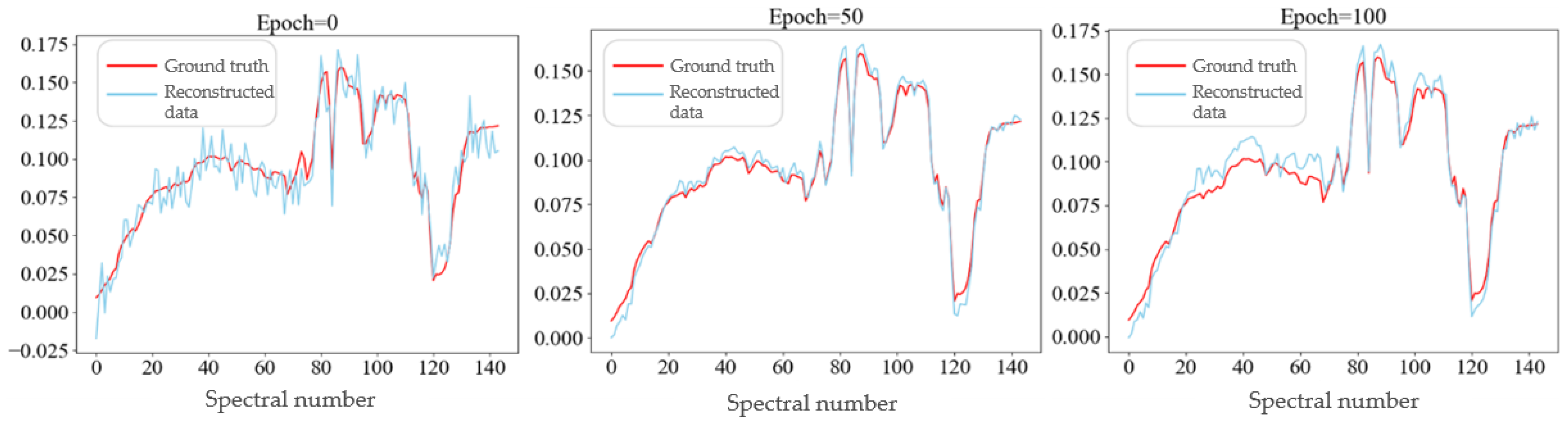
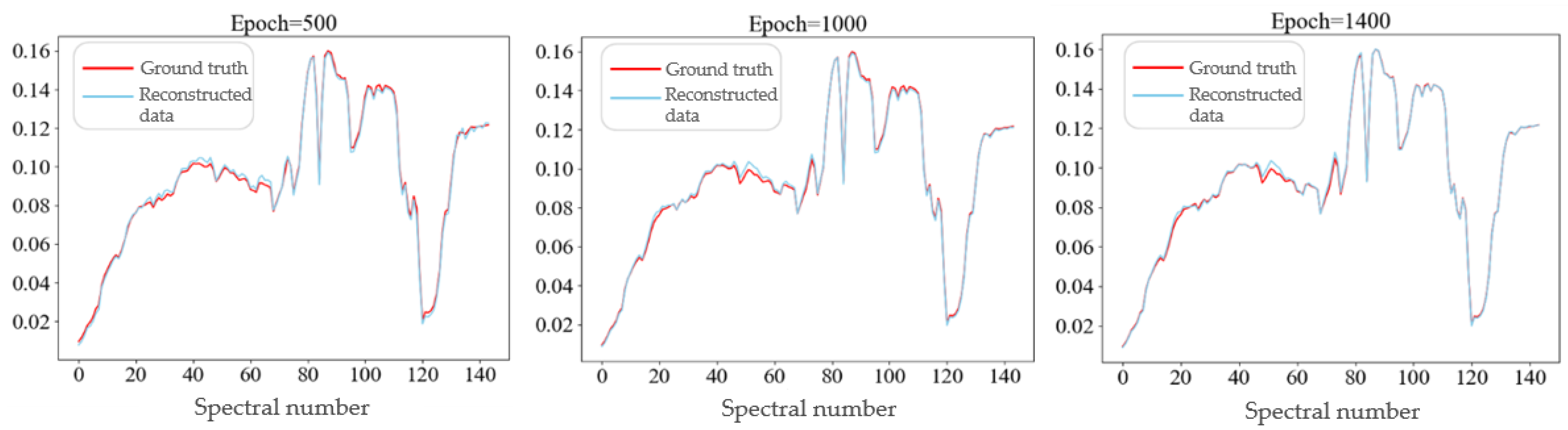
5.2. Analysis of the Training Process

The training and testing of the spectral super-resolution network use the Pytorch framework. During the training process, the batch size of the training data was set to eight, the parameter optimization algorithm was selected as Adam, and the parameter selection was optimized to ${\beta }_1=0.9$, ${\beta }_2=0.999$. Moreover, the learning rate was initialized to 4 × 10⁻⁴, and was adjusted by using the cosine annealing scheme based on 200 cycles. The target of the network was the MRAE loss function between the output image and the pseudo labels generated by the fusion module. As shown in Formula (27), $Y$ and $\widehat{Y}$ represent the test image and the reference image, respectively.

$$MRAE(Y,\widehat{Y})=\frac{1}{N}{\displaystyle \sum _{i=1}^N\frac{\left|Y[i]-\widehat{Y}[i]\right|}{Y[i]}}$$

(27)

Similarly, the training and testing of the adaptive learning network also use the Pytorch framework. During the training process, adaptive learning was performed on individual training data based on the given spectral response function. And the average absolute error as a loss function to output was set, which calculates the average error of each pixel between the HSI and MSI image. Moreover, the number of iterations for network training was set to 1500. In the adaptive module, the initial network parameters were randomly initialized, and the parameter optimization algorithm was selected as Adam. Furthermore, the learning rate was initialized to 9 × 10⁻⁵, and the learning rate weight setting was adjusted to 1 × 10⁻⁵. The size of the convolution kernel in the spatial degenerate network was 32 × 32. The parameters were initialized using a Gaussian template, and similarly, the parameter optimization algorithm was also selected as Adam, and the learning rate was initialized to 1 × 10⁻⁴, adjusting the weight to 1 × 10⁻³.

Figure 10a shows the variation in the loss of the spectral super-resolution network with the number of iterations. In the first 50 iterations, the loss of the network rapidly decreased to zero, and with the increase in iterations, the loss stabilized and became closer to zero. Similarly, Figure 10b shows the loss of the adaptive learning network varies with the number of iterations. And during the training process, the number of iterations was set to 1500. As the number of iterations increases, although the loss of the network still decreases to a certain extent, the efficiency of network improvement decreases, and the loss of the network gradually tends to stabilize.

Figure 11 represents the time required for training the spectral super-resolution network on different datasets. The network was trained on the TITAN Xp GPU, and the figure calculates the time required for each iteration in the first 50 iterations of the network. For Houston data, the average time taken for 50 iterations resulted in 122.95 s for each iteration. And, for GF-YR data, similarly, the average time was 190.22 s. During the training process of the adaptive learning network, the Houston data were cropped with 10 image blocks and the network had 1500 iterations. Moreover, the average training time for each image block was 335.06 s. And, for GF-YR, the training data were a single sheet size of 500 × 500. We also set the number of iterations to 1500, and the network training took 4339 s.

As shown in Figure 12, the spectral curves of a fixed pixel on Houston data achieve a comparative analysis between the reconstructed image and the real HS image during the training iteration process of the adaptive learning network, where the blue curve shows the pixels from the reconstructed image, and the red curve shows the pixels on the real HSI. At the initial iteration, there is a significant deviation between the output of the network and the real HSI. However, due to learning from the training data in the spectral super-resolution network, the reconstructed data curve is roughly similar to the true curve, where there is a lot of noise.

With the iteration of the adaptive learning network, the residual learning between the reconstructed image and the real HSI is achieved, and the output spectral curve of the network gradually approaches the real HS image. In particular, in the first 10 iterations of the network, there is a significant improvement in the output image; when the number of iterations is 100, the network output reaches a high degree of overlap with the real HSI; and when the number of iterations is 1000, the output of the network basically coincides with the spectral curve of the real HSI, and has fine reconstruction results in the spectral range of 364~1046 nm.

5.3. Comparative Experiment and Analysis

In the experiment, reconstruction tests were conducted on the cropped image blocks. Owing to the overlapping areas between different image blocks, the output image needed to be concatenated. At the same time, the pixel values of the overlapping areas were determined by taking the average value.

Figure 13 shows the reconstruction and classification results of the Houston data, where (a) is a false-color display of the Houston original HS image, and (b) is a false-color display of the reconstructed image, where 71, 39, and 16 bands were selected as RGB. The model introduced spectral response priors through adaptive learning, and consequently, the reconstructed image was given a function of spectral preservation. Moreover, Figure 13c shows the results of using the SVM classifier to classify the reconstructed data, and the number of labels for the training sets and test sets of the various classes during the classification process are shown in Table 2.

As shown in Figure 14, we compare the spectral curves of various categories between the reconstructed data and the real HS data. Figure 14a–f respectively depict the spectral curves of six cover categories: Grass healthy, Synthetic Grass, Soil, Water, Tennis Court, and Running Track. And, specifically, the red curve represents the spectral curve of the corresponding pixel in the real HS image, and the blue one represents the spectral curve of the reconstruction results in the same pixel. In particular, it can be seen that although some deviation occurs, the spectral curve basically fits, and the evaluation index of the spectral loss (SAM) is 1.2894.

For the reconstruction image of the Houston data, an SVM classifier was used for classification. The number of labels used in the training and testing sets for each category is shown in Table 2. And, eventually, we can obtain the confusion matrix shown in Figure 15, and the overall accuracy of classification is 76.53%. The highest accuracy for a single category is 99%, which is the sixth category, and the land feature is water.

In the confusion matrix, the row coordinates represent the category of the input image, and the column coordinates represent the category of network prediction. Moreover, the values in the grid show the proportion of the situation represented by the coordinates in the total number of data in this category, and the depth of the color in the grid represents the size of the grid value.

For the GF-YR data, the reconstructed hyperspectral data include 295 bands. As shown in Figure 16b, selecting bands 56, 39, and 25 for a false-color display can obtain the reconstructed image, which has a certain degree of spectral preservation on the selected three bands, and the color presented is basically consistent with the real HSI. Moreover, Figure 16c shows the result of classifying reconstructed images by using the KNN classifier, and the overall classification accuracy is 82.51%.

Table 4. Evaluation indicators for reconstruction results in the Houston dataset.

	PSNR	SAM (°)	SSIM	OA	DS	Dλ	QNR
Proposed	43.5576	1.2894	0.9996	0.7653	0.0170	0.0074	0.9756
J-SLoL [18]	35.0719	5.5209	0.9699	0.6764	0.0374	0.0622	0.9027
MPRNet [26]	34.6842	4.2354	0.9541	0.6896	0.0694	0.0781	0.8579
CGCDL [20]	35.5778	4.7765	0.9977	0.6907	0.0364	0.1106	0.8570
MSSNet [22]	31.2342	3.0510	0.9367	0.6975	0.0518	0.1174	0.8367

and

Table 5. Evaluation indicators for reconstruction results in the GF-YR dataset.

	OA	DS	Dλ	QNR
Proposed	0.8251	0.0471	0.0549	0.9004
J-SLoL [18]	0.7815	0.1218	0.1667	0.7317
MPRNet [26]	0.7726	0.1496	0.1238	0.7451
CGCDL [20]	0.8636	0.1803	0.1772	0.6744
MSSNet [22]	0.7842	0.1121	0.1614	0.7451

represent the evaluation index of the reconstruction results in different methods of the Houston and GF-YR data, respectively, and the highlighted data are the best indicator among the various methods. Specifically, J-SLoL [18], MPRNet [26], CGCDL [20], and MSSNet [22] are used as comparison methods, where J-SLoL and CGCDL are dictionary learning methods, and MPRNet and MSSNet are deep learning methods. In order to ensure a fair comparison and highlight the effectiveness of the proposed method, we opted for the same training and testing dataset to conduct a comparison test. In J-SLoL and CGCDL, we traversed the different atomic numbers of the dictionary, and finally selected the image with the best reconstruction effect for index calculation; and, in MPRNet and MSSNet, where the network ran on TITAN Xp GPU, the parameter optimization algorithm was also selected as Adam, and the initial learning rate was 2 × 10⁻⁴, which steadily decreased to 1 × 10⁻⁶ using the cosine annealing strategy.

In Table 4 and Table 5, the various indexes of the proposed method were significantly improved compared with the comparison methods. For the Houston data, the proposed method improved PSNR by 6.4482, and classification accuracy increased by 2.78%. For the GF-YR, the classification accuracy of the reconstructed model improved by 2.59%, and the global image quality evaluation index QNR improved by 0.1661.

However, for the GF data, the overall accuracy (OA) in classification is slightly lower than CGCDL, which could be due to CGCDL’s focus on classifying reconstructed images, neglecting spectral super-resolution. Consequently, while CGCDL achieves high classification accuracy, its spectral and spatial authenticity is slightly compromised. In contrast, our proposed method effectively balances the similarity of image reconstruction with high classification accuracy, delivering impressive results on both Houston and GF datasets.

5.4. Ablation Experiments on Partial Network Structures

In the multispectral–hyperspectral collaborative mapping model based on adaptive learning, the adaptive learning network introduces spectral response priors and learns the specific spatial degradation functions of the image. And, then, through the spatial degradation network and the given spectral response function, the preliminarily reconstructed image is mapped to the original HSI and MSI, respectively. The residual is adjusted pixel by pixel and, thus, the details of the image are refined to complete the unsupervised adaptive learning. The image fusion module provides pseudo labels for the training of spectral super-resolution networks based on training HSI and MSI, enabling the network to learn the mapping between HSI and MSI in a supervised manner. In order to verify the performance of some modules in the network, this section conducted ablation experiments on the following two network structures: the adaptive learning module and the image fusion module. Particularly, in the ablation experiment of the image fusion module, the module is replaced by a bilinear interpolation operation.

As shown in Figure 17, the reconstructed spectral curves of some categories before and after adaptive learning for GF-YR data are represented, where (a–f) respectively depict the spectral curves of six categories: Reed, Tidal Reed, Saltmarsh, Bare Tidal Flats, Water, and Spartina Alterniflora. Specifically, the red curve in the figure represents the spectra of corresponding pixels in the real HS image. Moreover, the blue curve represents the output of the network before adaptive learning, and the yellow curve represents the spectra of the same pixels in the reconstruction results of the network after adaptive learning. It can be seen that before the adaptive learning, although the output of the network’s spectral curve roughly follows the curve of the real HSI, there is still a certain offset. And noise is generated in some bands, causing the network to produce more spikes. Whereas, after the adaptive learning, the fitting of spectral curves further improves, and finally, has fine reconstruction results in the 295 spectral bands with the spectral range of 400~2500 nm.

As shown in

Table 6. Comparison of evaluation indicators for reconstruction results of ablation experiments on the Houston dataset.

Methods	PSNR	SAM (°)	SSIM	OA	DS	Dλ	QNR
w/o adaptation	40.9896	1.3752	0.9997	0.7480	0.0164	0.0094	0.9741
w/o fusion	36.6576	3.2535	0.9538	0.7644	0.0331	0.0345	0.9315
Proposed	43.5576	1.2894	0.9996	0.7653	0.0170	0.0074	0.9756

and

Table 7. Comparison of evaluation indicators for reconstruction results of ablation experiments on the GF-YR dataset.

Methods	OA	DS	Dλ	QNR
w/o adaptation	0.8150	0.0736	0.0552	0.8752
w/o fusion	0.8077	0.1726	0.1259	0.7232
Proposed	0.8251	0.0471	0.0549	0.9004

, the comparison of the evaluation indicators for the adaptive learning network and the ablation experiment of the image fusion module is represented, where w/o adaptation represents the reconstruction results of the model after removing the adaptive learning network, and w/o fusion represents the reconstruction results of the model after removing the image fusion module. Specifically, in the Houston data, the adaptive learning network improves the SNR, spectral loss, and classification accuracy of the reconstruction image by using spectral response priors. Although the spatial evaluation index is slightly reduced, the overall reconstruction effect is better. Moreover, the fusion module obviously improves the SNR by 6.9, and the spectral loss evaluation index SAM is improved by 2.9641, which obviously improves the reconstruction quality of the network. Similarly, for the GF-YR data, both modules can improve classification accuracy and the unsupervised spatial and spectral evaluation indexes.

6. Conclusions

For multispectral–hyperspectral collaborative mapping and refined classification tasks, in order to avoid the complex parameter selection based on dictionary learning, a collaborative mapping model based on adaptive learning is constructed, which provides the required pseudo labels through a fusion module. Moreover, we design an adaptive learning network to increase the spectral response prior and learn the unknown spatial degradation function, so as to further improve the quality of the reconstructed image. Then, ablation experiments are designed to verify the effectiveness of the relevant network structures. Finally, we obtain the conclusion that the classification accuracy of reconstruction results in the mapping model based on adaptive learning improved by 2.78% and 2.59% in the two datasets: Houston and GF-YR, respectively.

The innovation of this paper is the design of the adaptive learning-based multi-hyperspectral collaborative mapping model. A physical model embedding is realized by designing an adaptive learning network to introduce the spectral response function, which further guides the high precision of spectral reconstruction. Specifically, using the adaptive learning module to incorporate spectral response priors that adjust the output of the super-resolution network to preserve spectral information in reconstructed data, and the attention-based model, has advantages in capturing the characteristics conducive to spectral super-resolution. The image fusion module leverages spatial and spectral consistency in training data, providing pseudo labels for spectral super-resolution training. The implementation of these modules can significantly enhance the quality and precision of reconstruction.

In addition, there are still some issues worth considering and researching in relation to the content of this article: in the mapping model based on adaptive learning, adding an image fusion block to the training process of the model should be considered to further improve the learning ability.

References

1. Li, M.; Luo, Q.; Liu, S. Application of Hyperspectral Imaging Technology in Quality Inspection of Agricultural Products. In Proceedings of the 2022 International Conference on Computers, Information Processing and Advanced Education (CIPAE), Ottawa, ON, Canada, 26–28 August 2022; pp. 369–372. [Google Scholar]
2. Rayhana, R.; Ma, Z.; Liu, Z.; Xiao, G.; Ruan, Y.; Sangha, J.S. A Review on Plant Disease Detection Using Hyperspectral Imaging. IEEE Trans. AgriFood Electron. 2023, 1, 108–134. [Google Scholar] [CrossRef]
3. Tang, X.-J.; Liu, X.; Yan, P.-F.; Li, B.-X.; Qi, H.-Y.; Huang, F. An MLP Network Based on Residual Learning for Rice Hyperspectral Data Classification. IEEE Geosci. Remote Sens. Lett. 2022, 19, 6007405. [Google Scholar] [CrossRef]
4. Zhou, Q.; Wang, S.; Guan, K. Advancing Airborne Hyperspectral Data Processing and Applications for Sustainable Agriculture Using RTM-Based Machine Learning. In Proceedings of the IGARSS 2023, 2023 IEEE International Geoscience and Remote Sensing Symposium, Pasadena, CA, USA, 16–21 July 2023; pp. 1269–1272. [Google Scholar]
5. Oudijk, A.E.; Hasler, O.; Øveraas, H.; Marty, S.; Williamson, D.R.; Svendsen, T.; Berg, S.; Birkeland, R.; Halvorsen, D.O.; Bakken, S.; et al. Campaign For Hyperspectral Data Validation In North Atlantic Coastal Waters. In Proceedings of the 2022 12th Workshop on Hyperspectral Imaging and Signal Processing: Evolution in Remote Sensing (WHISPERS), Rome, Italy, 13–16 September 2022; pp. 1–5. [Google Scholar]
6. Rocha, A.D.; Groen, T.A.; Skidmore, A.K.; Willemen, L. Role of Sampling Design when Predicting Spatially Dependent Ecological Data With Remote Sensing. IEEE Trans. Geosci. Remote Sens. 2021, 59, 663–674. [Google Scholar] [CrossRef]
7. Guo, T.; Luo, F.; Guo, J.; Duan, Y.; Huang, X.; Shi, G. Hyperspectral Target Detection With Target Prior Augmentation and Background Suppression-Based Multidetector Fusion. IEEE J. Sel. Top. Appl. Earth Obs. Remote Sens. 2024, 17, 1765–1780. [Google Scholar] [CrossRef]
8. Qi, J.; Gong, Z.; Xue, W.; Liu, X.; Yao, A.; Zhong, P. An Unmixing-Based Network for Underwater Target Detection From Hyperspectral Imagery. IEEE J. Sel. Top. Appl. Earth Obs. Remote Sens. 2021, 14, 5470–5487. [Google Scholar] [CrossRef]
9. Sun, L.; Ma, Z.; Zhang, Y. ABLAL: Adaptive Background Latent Space Adversarial Learning Algorithm for Hyperspectral Target Detection. IEEE J. Sel. Top. Appl. Earth Obs. Remote Sens. 2024, 17, 411–427. [Google Scholar] [CrossRef]
10. Wang, S.; Feng, W.; Quan, Y.; Bao, W.; Dauphin, G.; Gao, L.; Zhong, X.; Xing, M. Subfeature Ensemble-Based Hyperspectral Anomaly Detection Algorithm. IEEE J. Sel. Top. Appl. Earth Obs. Remote Sens. 2022, 15, 5943–5952. [Google Scholar] [CrossRef]
11. Bai, W.; Zhang, P.; Liu, H.; Zhang, W.; Qi, C.; Ma, G.; Li, G. A Fast Piecewise-Defined Neural Network Method to Retrieve Temperature and Humidity Profile for the Vertical Atmospheric Sounding System of FengYun-3E Satellite. IEEE Trans. Geosci. Remote Sens. 2023, 61, 4100910. [Google Scholar] [CrossRef]
12. Fiscante, N.; Addabbo, P.; Biondi, F.; Giunta, G.; Orlando, D. Unsupervised Sparse Unmixing of Atmospheric Trace Gases From Hyperspectral Satellite Data. IEEE Geosci. Remote Sens. Lett. 2022, 19, 6006405. [Google Scholar] [CrossRef]
13. Wang, J.; Li, C. Development and Prospect of Hyperspectral Imager and Its Application. Chin. J. Space Sci. 2021, 41, 22–33. [Google Scholar] [CrossRef]
14. Arad, B.; Ben-Shahar, O. Sparse recovery of hyperspectral signal from natural RGB images. In Proceedings of the European Conference on Computer Vision, Amsterdam, The Netherlands, 8–16 October 2016; pp. 19–34. [Google Scholar]
15. Wu, J.; Aeschbacher, J.; Timofte, R. In Defense of Shallow Learned Spectral Reconstruction from RGB Images. In Proceedings of the 2017 IEEE International Conference on Computer Vision Workshops (ICCVW), Venice, Italy, 22–29 October 2017; pp. 471–479. [Google Scholar]
16. Yokoya, N.; Heiden, U.; Bachmann, M. Spectral Enhancement of Multispectral Imagery Using Partially Overlapped Hyperspectral Data and Sparse Signal Representation. In Proceedings of the Whispers 2018, Amsterdam, The Netherlands, 24–26 September 2018. [Google Scholar]
17. Fotiadou, K.; Tsagkatakis, G.; Tsakalides, P. Spectral Super Resolution of Hyperspectral Images via Coupled Dictionary Learning. IEEE Trans. Geosci. Remote Sens. 2019, 57, 2777–2797. [Google Scholar] [CrossRef]
18. Gao, L.; Hong, D.; Yao, J.; Zhang, B.; Gamba, P.; Chanussot, J. Spectral Superresolution of Multispectral Imagery With Joint Sparse and Low-Rank Learning. IEEE Trans. Geosci. Remote Sens. 2021, 59, 2269–2280. [Google Scholar] [CrossRef]
19. Han, X.; Yu, J.; Luo, J.; Sun, W. Reconstruction From Multispectral to Hyperspectral Image Using Spectral Library-Based Dictionary Learning. IEEE Trans. Geosci. Remote Sens. 2019, 57, 1325–1335. [Google Scholar] [CrossRef]
20. Liu, T.; Gu, Y.; Jia, X. Class-guided coupled dictionary learning for multispectral-hyperspectral remote sensing image collaborative classification. Sci. China Technol. Sci. 2022, 65, 744–758. [Google Scholar] [CrossRef]
21. Liu, T.; Gu, Y.; Yu, W.; Jia, X.; Chanussot, J. Separable Coupled Dictionary Learning for Large-Scene Precise Classification of Multispectral Images. IEEE Trans. Geosci. Remote Sens. 2022, 60, 5542214. [Google Scholar] [CrossRef]
22. Yan, Y.; Zhang, L.; Li, J.; Wei, W.; Zhang, Y. Accurate Spectral Super-Resolution from Single RGB Image Using Multi-scale CNN. In Pattern Recognition and Computer Vision, In Proceedings of the First Chinese Conference, PRCV 2018, Guangzhou, China, 23–26 November 2018; Lecture Notes in Computer Science; Lai, J.-H., Liu, C.-L., Chen, X., Zhou, J., Tan, T., Zheng, N., Zha, H., Eds.; Springer: Cham, Switzerland, 2018; pp. 206–217. [Google Scholar]
23. Han, X.; Zhang, H.; Xue, J.-H.; Sun, W. A Spectral–Spatial Jointed Spectral Super-Resolution and Its Application to HJ-1A Satellite Images. IEEE Geosci. Remote Sens. Lett. 2022, 19, 5505905. [Google Scholar] [CrossRef]
24. Hu, X.; Cai, Y.; Lin, J.; Wang, H.; Yuan, X.; Zhang, Y.; Timofte, R.; Van Gool, L. Hdnet: High-resolution dual-domain learning for spectral compressive imaging. In Proceedings of the IEEE/CVF Conference on Computer Vision and Pattern Recognition, New Orleans, LA, USA, 18–24 June 2022; pp. 17542–17551. [Google Scholar]
25. Li, J.; Du, S.; Song, R.; Wu, C.; Li, Y.; Du, Q. HASIC-Net: Hybrid Attentional Convolutional Neural Network With Structure Information Consistency for Spectral Super-Resolution of RGB Images. IEEE Trans. Geosci. Remote Sens. 2022, 60, 5522515. [Google Scholar] [CrossRef]
26. Zamir, S.W.; Arora, A.; Khan, S.; Hayat, M.; Khan, F.S.; Yang, M.-H.; Shao, L. Multi-Stage Progressive Image Restoration. In Proceedings of the 2021 IEEE/CVF Conference on Computer Vision and Pattern Recognition (CVPR), Nashville, TN, USA, 20–25 June 2021; pp. 14816–14826. [Google Scholar]
27. Li, J.; Du, S.; Wu, C.; Leng, Y.; Song, R.; Li, Y. DRCR Net: Dense Residual Channel Re-calibration Network with Non-local Purification for Spectral Super Resolution. In Proceedings of the 2022 IEEE/CVF Conference on Computer Vision and Pattern Recognition Workshops (CVPRW), New Orleans, LA, USA, 19–20 June 2022; pp. 1258–1267. [Google Scholar]
28. He, J.; Yuan, Q.; Li, J.; Xiao, Y.; Liu, X.; Zou, Y. DsTer: A dense spectral transformer for remote sensing spectral super-resolution. Int. J. Appl. Earth Obs. Geoinf. 2022, 109, 102773. [Google Scholar] [CrossRef]
29. Li, T.; Liu, T.; Li, X.; Gu, Y.; Wang, Y.; Chen, Y. Multi-sensor Multispectral Reconstruction Framework Based on Projection and Reconstruction. Sci. China Inf. Sci. 2024, 67, 132303. [Google Scholar] [CrossRef]
30. Li, T.; Gu, Y. Progressive Spatial–Spectral Joint Network for Hyperspectral Image Reconstruction. IEEE Trans. Geosci. Remote Sens. 2022, 60, 5507414. [Google Scholar] [CrossRef]
31. Li, T.; Liu, T.; Wang, Y.; Li, X.; Gu, Y. Spectral Reconstruction Network From Multispectral Images to Hyperspectral Images: A Multitemporal Case. IEEE Trans. Geosci. Remote Sens. 2022, 60, 5535016. [Google Scholar] [CrossRef]
32. Du, D.; Gu, Y.; Liu, T.; Li, X. Spectral Reconstruction From Satellite Multispectral Imagery Using Convolution and Transformer Joint Network. IEEE Trans. Geosci. Remote Sens. 2023, 61, 5515015. [Google Scholar] [CrossRef]
33. Aiazzi, B.; Alparone, L.; Baronti, S.; Garzelli, A.; Selva, M. MTF-tailored Multiscale Fusion of High-resolution MS and Pan Imagery. Photogramm. Eng. Remote Sens. 2006, 72, 591–596. [Google Scholar] [CrossRef]
Figure 1. The structure of collaborative mapping model based on adaptive learning.
Remotesensing 16 01384 g001
Figure 2. The structure of spectral super-resolution network based on self-attention mechanism: (a) Spectral super-resolution network; (b) Single-stage spectral transformation module (SST).
Remotesensing 16 01384 g002
Figure 3. The spectral self-attention module (SAB): (a) The specific structure of SAB; (b) The structure of the feedforward network in SAB.
Remotesensing 16 01384 g003
Figure 4. The spectral multi-headed self-attention module (S-MSA).
Remotesensing 16 01384 g004
Figure 5. Self-adaptive learning network.
Remotesensing 16 01384 g005
Figure 6. The structure of self-guided block.
Remotesensing 16 01384 g006
Figure 7. The Houston data: (a) The false-color display (selecting 71, 39, and 16 bands); (b) Labels of the training set; (c) Labels of the test set; (d) All feature categories.
Remotesensing 16 01384 g007
Figure 8. The GF-YR data: (a) The false-color display (selecting 56, 39, and 25 bands); (b) Classification diagram; (c) All feature categories.
Remotesensing 16 01384 g008
Figure 9. A portion of the Houston training data.
Remotesensing 16 01384 g009
Figure 10. The training process of the network: (a) The training process of the spectral super-resolution network; (b) The training process of the self-adaptive learning network.
Remotesensing 16 01384 g010
Figure 11. The time required for the training process of spectral super-resolution network.
Remotesensing 16 01384 g011
Figure 12. The variation in spectral curve with the number of iterations in adaptive learning network.
Remotesensing 16 01384 g012aRemotesensing 16 01384 g012b
Figure 13. The reconstruction and classification image of Houston data: (a) The real HS image of Houston data; (b) The reconstruction image of Houston data; (c) the results of using SVM classifier; (d) All feature categories.
Remotesensing 16 01384 g013
Figure 14. The spectral curves of various categories between the Houston reconstruction data and the truth data: (a) Grass healthy; (b) Synthetic Grass; (c) Soil; (d) Water; (e) Tennis court; (f) Running Track.
Remotesensing 16 01384 g014
Figure 15. The confusion matrix of the Houston classification results.
Remotesensing 16 01384 g015
Figure 16. The reconstruction and classification results of GF-YR data: (a) The real HS image of GF-YR; (b) The reconstruction HSI of GF-YR; (c) The classification results of GF-YR; (d) All feature categories.
Remotesensing 16 01384 g016
Figure 17. The reconstructed spectral curves of some categories before and after adaptive learning for GF-YR data: (a) Reed; (b) Tidal Reed; (c) Saltmarsh; (d) Bare Tidal Flats; (e) Water; (f) Spartina Alterniflora.
Remotesensing 16 01384 g017