Abstract
The increasing incidence of retrogressive thaw slumps (RTSs) in permafrost regions underscores the need for detailed spatial and temporal analysis using InSAR technology to monitor and predict dynamic changes in the process of RTSs. Nevertheless, current InSAR deformation forecasting methods employing deep learning strategies such as the traditional long short-term memory (LSTM) and recent transformer models encounter difficulties in effectively capturing temporal features. Moreover, they are limited in their ability to directly integrate spatial information. In this paper, an innovative deep learning approach named Spacetimeformer is proposed for predicting medium- and short-term InSAR deformation of RTSs in the Chumar River area. This method employs a transformer architecture with a spatiotemporal attention mechanism, which enhances the long-term prediction capabilities of time series models and dynamic spatial modeling. It is applicable to multivariate InSAR spatiotemporal deformation prediction problems. The findings include a list of 72 RTSs compiled based on derived InSAR deformation maps and Sentinel-2 optical images, of which 64 have an average deformation rate exceeding 10 mm/year, indicating signs of permafrost degradation. The density distribution of the displacement maps predicted by the Spacetimeformer model aligned well with the InSAR deformation maps obtained from the small baseline subset (SBAS) method, with the overall prediction deviation controlled within 20 mm. In addition, the point-scale prediction results were compared with LSTM and transformer models. This study indicates that the Spacetimeformer network achieved good results in predicting the deformation of RTSs, with a root mean square error of 1.249 mm. The Spacetimeformer method for deformation prediction with the spacetime mechanism presented in this study can serve as a general framework for multivariate deformation prediction based on InSAR results. It can also quantitatively assess the spatial deformation characteristics and deformation trends of RTSs.
1. Introduction
The permafrost on the Qinghai–Tibet Plateau (QTP) covers an area of approximately 1.06 × 10⁶ km2 (with temperatures lower than −2 °C) [1], and it is particularly sensitive and vulnerable to global warming and human activities [2]. Currently, the central region of the QTP is undergoing rapid and substantial permafrost degradation, marked by rising ground temperatures, an expanding active layer, contracting extent, decreasing thickness, and an ascending lower boundary [3]. Retrogressive thaw slumps (RTSs), among the most dynamic geomorphological features in the QTP’s permafrost zones, are experiencing accelerated melting and erosion from the warming of global permafrost, particularly due to extensive melting of ice-rich permafrost. This not only alters the landscape and ecosystem of the Qinghai–Tibet Plateau but also potentially accelerates the release of soil organic carbon, which could undermine infrastructure stability and impact the global carbon cycle and climate change [4,5,6]. Understanding the surface deformation characteristics and future trends of these thaw slumps across spatial and temporal dimensions is crucial. Additionally, conducting comprehensive studies on the spatiotemporal patterns of surface deformation, exploring large-scale deformation mapping possibilities, and assessing future trends, remain equally essential. [7]. Therefore, deformation monitoring and mid-short-term prediction techniques for RTSs are significant in assessing the deformation trends of thaw slumps and the stability of infrastructure in cold regions. In recent decades, interferometric synthetic aperture radar (InSAR) technology, capable of measuring surface deformation with centimeter to subcentimeter precision and offering high spatial resolution and wide coverage in all weathers, has provided a powerful method for monitoring ground deformation in permafrost areas [8]. Additionally, the open data policy of the Sentinel-1 satellite has facilitated the application of InSAR technology for large-scale deformation measurement in permafrost areas. Alternatively, multi-temporal InSAR techniques (MT-InSAR) such as permanent scatterer interferometry (PSI) [9] and small baseline subset (SBAS) [10] have been successfully used to monitor seasonal changes and interannual surface elevation changes in permafrost areas of the QTP [11,12,13,14]. These studies have effectively monitored the freeze–thaw cycles of permafrost on the QTP, including combining seasonal deformation data with the Stefan model to invert the thickness of the active layer [15,16].
InSAR deformation prediction employing time-series modeling techniques aids significantly in enhancing capabilities for the monitoring and forecasting of geological disasters and regressive thaw slumps on the QTP. Currently, time series modeling has found extensive applications in fields such as climate modeling [17], biological sciences [18], and medicine [19], as well as retail and finance [20]. Traditional methods in time series modeling focus on parameter models informed by domain expertise [21]. These models are data-driven approaches, including autoregression (AR) [22], exponential smoothing [23], or structural time-series models [24]. Prior research has employed data-driven approaches like hyperbolic and gray–Markov models to forecast deformation data from InSAR. [25,26]. Model-driven approaches such as the probabilistic integral method, Kalman filtering, gray system theory models, and nonlinear least squares [27] rely on InSAR deformation results and other time-series data to achieve high-precision and reliable ground deformation prediction results. However, these traditional methods have poor applicability and usually require expert knowledge to manually select and adjust parameters [28], making it difficult to effectively handle the complex or nonlinear time-series deformation data patterns of permafrost. Modern machine learning methods offer a purely data-driven approach to learning time dynamics [29]. Recently, deep learning has revolutionized time-series prediction tasks through its exceptional ability to manage nonlinear patterns, automate feature extraction, and analyze extensive datasets. Convolutional neural network (CNN) techniques have successfully detected slow volcanic movements and predicted short-term InSAR deformation [30,31]. In particular, recurrent neural networks (RNNs) and long short-term memory (LSTM) networks have demonstrated substantial advantages in capturing complex dependencies and dynamic changes within time-series data. In 2021, Nukala et al. introduced an innovative approach using RNNs to predict time-series deformation maps with Sentinel-1 data [32]. The adoption of LSTM networks effectively addressed the issues of gradient explosion and vanishing that plagued earlier RNN variants in learning long-term data dependencies. This enhancement significantly improved the network’s capacity to learn long-term data dependencies. In their respective studies, Chen et al. (2021), Hill et al. (2021), and Bao et al. (2022) developed LSTM models tailored to time-series InSAR deformation, consistently demonstrating superior predictive performance over earlier methods [33,34,35]. Aoqing et al. (2022) presented a landslide prediction method based on a neural basis expansion analysis (N-BEATS) network model and achieved medium- and short-term landslide prediction by exploiting MTInSAR observations with a root mean square error accuracy of 1.1 mm [27]. Wang et al. utilized multivariate meteorological and hydrological data along with time-series InSAR deformation data through an enhanced transformer model to predict linear and seasonal displacement patterns in the QTP’s Salt Lake area, achieving an average point-scale accuracy of 6.71 mm [36]. Yao et al. and Yi et al. proposed a spatiotemporal prediction method for ground subsidence using a convolutional long short-term memory (ConvLSTM) neural network, effectively capturing both temporal features and spatial neighborhood characteristics [37,38].
However, previous studies have mainly focused on InSAR time-series deformation prediction methods based on CNN or LSTM models. These methods have shortcomings in capturing temporal features and considering spatial neighborhood characteristics, leading to poor reliability in spatiotemporal prediction of ground subsidence. Additionally, there has been limited research on multivariate time series deformation prediction using InSAR technology, which has primarily focused on using historical data to predict future values. Despite the latest sequence-to-sequence models relying on time-step attention mechanisms in neural networks for temporal learning, they fail to fully consider the complex spatial relationships between variables.
In this study, we propose a novel InSAR time series deformation prediction method employing the Spacetimeformer network model designed for multivariate InSAR deformation datasets, specifically applied to RTSs in the Chumar River Basin. The Spacetimeformer model proposed in this paper is a highly valuable addition to InSAR deformation prediction. The objectives of this paper are as follows: (1) to deduce the dynamic change processes of the RTSs in the Chumar River Basin using the introduced Spacetimeformer deformation prediction method, and (2) to map the RTSs areas in the Chumar River Basin and discuss the spatiotemporal deformation patterns of permafrost degradation in the RTSs. Following the introduction, this paper outlines the study area and datasets in Section 2. Section 3 elaborates on a SBAS InSAR algorithm based on a seasonal model and the InSAR time series displacement forecasting method utilizing the multivariate Spacetimeformer model. Section 4 presents the InSAR deformation prediction results, along with a detailed analysis of the precise deformation properties of the RTSs. Discussions on the forecast performance of the Spacetimeformer model and the spatiotemporal variations in surface deformation in the Chumar River Basin are covered in Section 5. Finally, Section 6 concludes the paper and outlines avenues for further research.
2. Study Area and Datasets
2.1. Study Area
The study area is located in the northeastern part of the QTP in Qinghai Province, near the Hoh Xil region (see Figure 1a), with the Qinghai-Tibet Railway and highway to the east. The region is bounded by the Wulan Mountains to the north and the Kunlun Mountains to the south, mainly comprising high-altitude hills and moderately undulating mountains, with most areas above 4500 m in elevation (see Figure 1b). The terrain consists of rolling hills and shallow gullies [39]. The primary natural cover in the area comprises alpine meadows, grasslands, and deserts, interspersed with widespread periglacial landforms. The study area features a semi-arid continental climate, with average annual temperatures ranging from −10.0 °C to −4.1 °C and precipitation varying between 70.5 mm and 291.4 mm. The region exhibits high evaporation rates. Notably, Zhuonai Lake and Kusai Lake, typical glacier-fed lakes, along with Haidingnor and Salt Lake, mainly replenished by rainfall, derive their primary water sources from meltwater and precipitation, respectively [14,40,41]. Observations at the Hoh Xil station (QT01) from 2004 to 2017 showed an increase in the active layer thickness from 160 cm to 176 cm. As permafrost thaws, the melting of ground ice significantly increases the water content at the bottom of the active layer. Consequently, permafrost degradation has occurred in the study area in recent years [42].
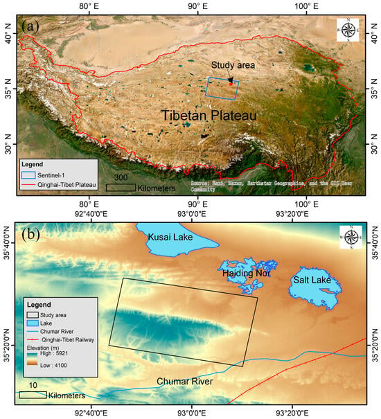
Figure 1.
Geographic location of the study area and coverage of Sentinel-1 data. (a) Sentinel-1 images and the study area superimposed on a color map of China; (b) the Chumar River area superimposed on Shuttle Radar Topography Mission (SRTM) digital elevation model (DEM) shaded topography map.
2.2. Datasets
2.2.1. Satellite Data
To acquire historical deformation data and predict future deformation trends in the study area, we collected 158 images from the terrain observation with progressive scans (TOPS) interferometric wide (IW) mode of the Sentinel-1A synthetic aperture radar (SAR). These images, utilizing VV polarization, spanned from 3 May 2018 to 4 October 2023. The Sentinel-1A satellite, launched on 3 April 2014, has a revisit cycle of 12 days and operates at a wavelength of approximately 5.6 cm. The images were captured along the descending orbit track T150. The swath width of the Sentinel-1A imagery was 250 km, with the line-of-sight (LOS) incidence angle varying between 31° and 46°.
Sentinel-2 optical imagery was utilized for delineating the boundaries of RTSs. The dataset comprised two Sentinel-2 acquisitions of multi-spectral instrument (MSI) level-1A data, specifically from 13 September 2023 and 15 August 2019 (as listed in Table 1). The selected images were from relative orbit number 133, capitalizing on the instrument’s wide swath width of 290 km and a high revisit frequency of 10 days at the equator with a single satellite from the Sentinel-2 mission.

Table 1.
Properties of Sentinel-1 and Sentinel-2 data used in this research.
2.2.2. Auxiliary Data
In this study, a 1-arc second resolution SRTM DEM with a ground resolution of 30 m was employed to simulate the topographic phase, which was then utilized for geocoding the InSAR deformation results [43]. Fifth-generation reanalysis data (ERA5) from the European Centre for Medium-Range Weather Forecasts (ECMWF) were used, and this study integrated 2 m dew-point temperature data from the monthly average reanalysis products of the ECMWF ERA5 [44], corresponding to the SAR image acquisition dates on a 0.25° × 0.25° grid. These data were used to establish the composite index deformation model and can be accessed at https://cds.climate.copernicus.eu/cdsapp#!/home (accessed on 19 May 2024).
3. Methodology
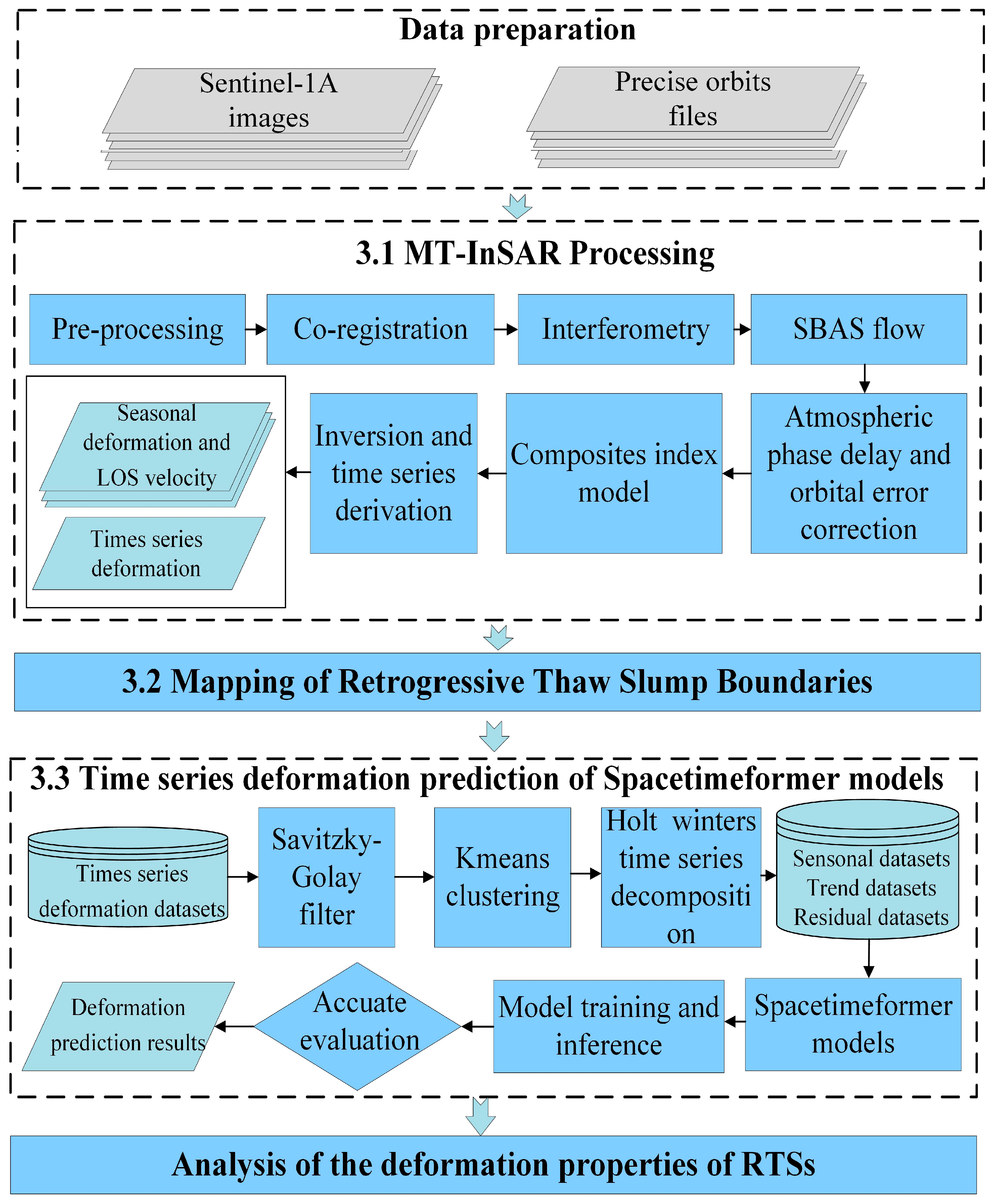
Figure 2 provides an overview and details the steps of this deformation prediction methodology. Initially, pre-processing and interferometry were conducted on the Sentinel-1 data. Seasonal deformation, LOS velocity, and time-series deformation of RTSs in the Chumar River area were calculated using the SBAS method based on a composite index model [36]. The RTSs areas were then mapped using the deformation results from SBAS combined with Sentinel-2 optical images. The InSAR time-series deformation results are preprocessed using the Savitzky–Golay (SG) filtering algorithm [45], and the InSAR time series deformation data of the study area were clustered into different deformation pattern datasets using the Kmeans algorithm [46]. The data from each InSAR measurement point were reorganized into one-dimensional time series, which were then decomposed using the Holt–Winters time-series decomposition method [47]. The Spacetimeformer multivariate time series spatiotemporal prediction model for different deformation patterns was constructed and applied to the time-series deformation prediction of the Chumar River’s RTSs. Finally, the prediction accuracy’s dependence on spatiotemporal mechanisms was assessed through comparing the results of the Spacetimeformer model, integrated with spatiotemporal concepts, against those of the LSTM and transformer models at the point scale.
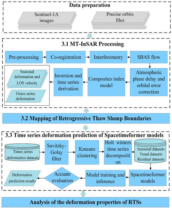
Figure 2.
Processing flow of Spacetimeformer time-series deformation prediction method. This figure depicts content related to Section 3.1, Section 3.2 and Section 3.3 in the text.
3.1. MT-InSAR Processing
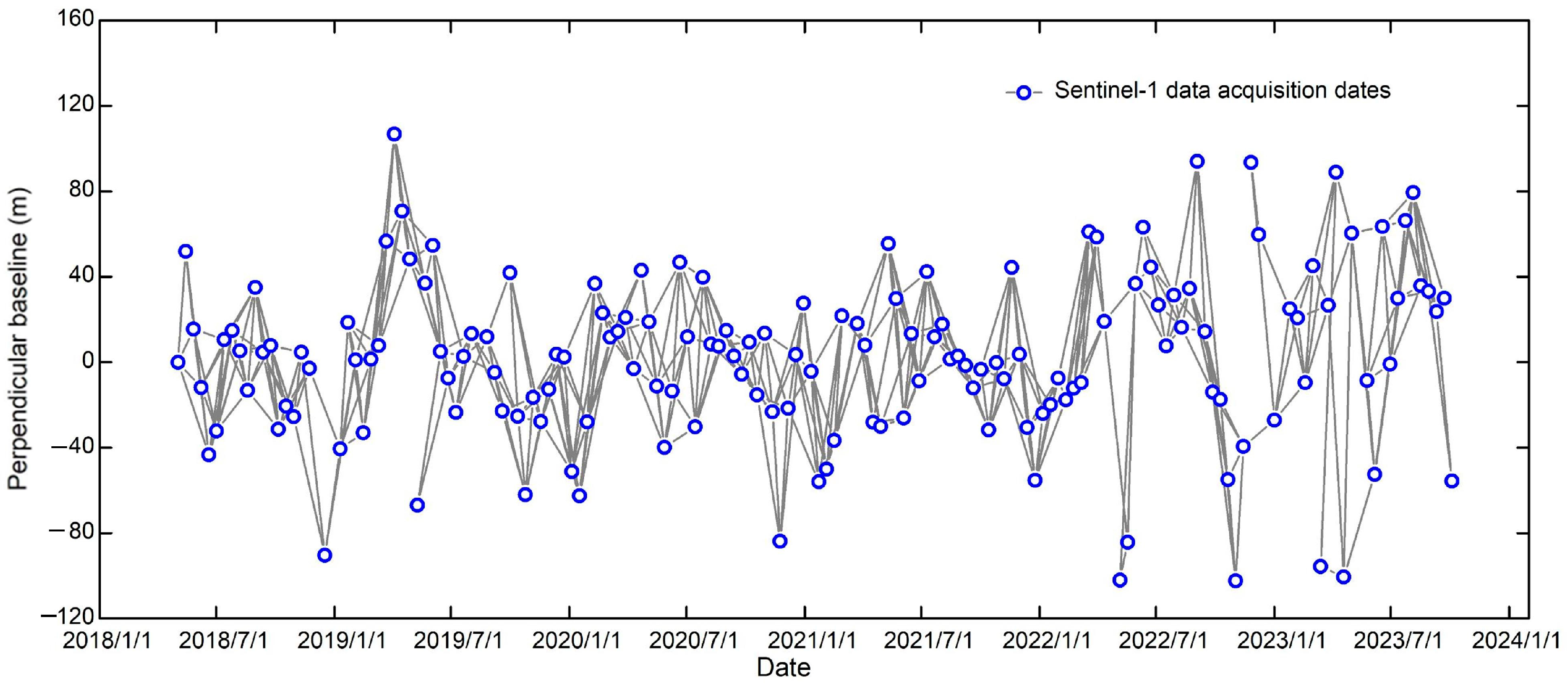
A total of 158 Sentinel-1 SAR images were processed using the SBAS method for time-series deformation calculation. Initially, precise orbital correction and DEM co-registration were implemented on the Sentinel-1 data, utilizing the enhanced spectral diversity (ESD) co-registration method to refine azimuth offsets in Sentinel-1 images [48]. De-ramping, interpolation, and re-ramping were performed on each burst [49], followed by mosaicking of all bursts on each strip, and then interferometric processing to produce interferograms. The interferograms were multi-looked in the range direction by a factor of 2 and in the azimuth direction by a factor of 12 to reduce noise. The 30 m DEM from the SRTM was used to remove contributions from flat-earth and topographic phases [50]. Differential interferometric pairs were selected with a temporal baseline threshold of 50 days and a spatial baseline threshold of 100 m, as indicated by the blue circles for SAR image acquisition dates and gray lines for a set of interferograms in Figure 3. Additionally, some interferograms affected by severe decorrelation and atmospheric phase delays were discarded. Ultimately, 498 Sentinel-1 interferograms were selected for MT-InSAR processing. Goldstein adaptive spatial filtering [51] was applied to each interferogram, and the minimum cost flow (MCF) method [52] was used to unwrap the differential interferometric phases. GMTSAR software (version 6.1) was used to implement the above steps [50].
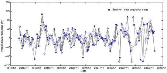
Figure 3.
Spatiotemporal baselines of the Sentinel-1 interferograms.
In this study, to precisely capture the RTSs’ deformation pattern in the permafrost, a composite index model was integrated into the SBAS algorithm for calculating time-series deformation [53]. The fifth-generation global climate reanalysis ERA5 data were utilized for atmospheric phase screen estimation. Atmospheric correction was applied to all unwrapped interferograms, and residual orbital errors in each interferogram were rectified using the network de-ramping method. Given that the study area is located in the hinterland of the Tibetan Plateau, we selected a reference point on the southern side of the mountain range within our study area, composed of stable bedrock. All movements within the study area were considered relative to this reference point. Finally, the SBAS inversion technique was employed to derive seasonal deformation changes and time-series displacement, and the GIAnT toolbox is adopted to execute the SBAS inversion [54].
3.2. Mapping of Retrogressive Thaw Slump Boundaries
After acquiring the ground deformation rate maps processed via SBAS, we integrated these results with Sentinel-2 optical imagery for visual interpretation of the RTSs. Initially, an LOS deformation rate threshold of 15 mm was set to delineate potential thaw slump areas. Time-series deformation data were employed to filter out deformations unrelated to permafrost degradation. Subsequently, suspected landslide areas were marked on multi-temporal Sentinel-2 optical remote sensing images and further verified using surface morphological features such as exposed sediments, newly exposed well walls, and sparse vegetation [4]. This was carried out to eliminate falsely identified landslide areas and achieve precise mapping. It is noteworthy that boundaries determined solely based on deformation characteristics may underestimate the actual extent of landslides, as some landslide areas might not exhibit significant deformation during the observation period [55]. Therefore, Sentinel-2 optical images were utilized in conjunction with InSAR measurements to accurately delineate the outer contours of the RTSs.
3.3. Time Series Deformation Prediction of Spacetimeformer Models
3.3.1. Dataset Preprocessing and Holt–Winters Time-Series Decomposition
In this study, 588,600 InSAR measurement points with coherence greater than 0.30 in the time-series deformation map were selected and reorganized into time-series data. The time-series deformation data were clustered using the Kmeans algorithm to establish time-series deformation datasets for each category [56]. The Spacetimeformer network was then used to construct deformation prediction models for each category of RTSs.
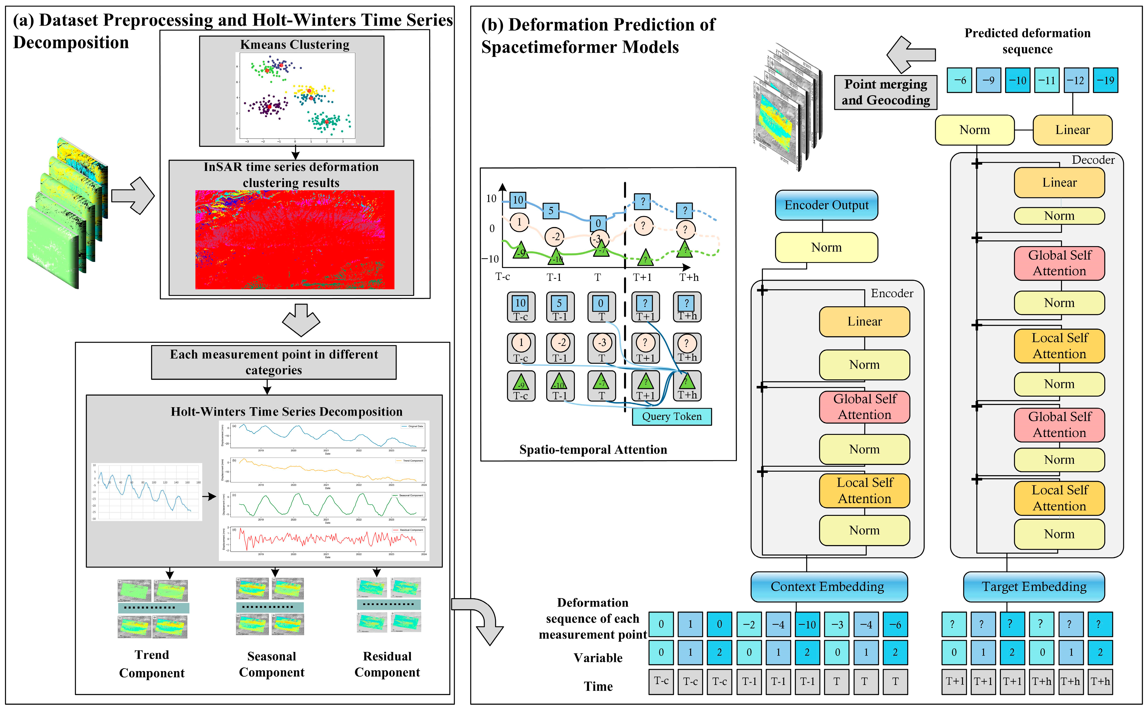
To better predict the future time-series deformation of RTSs in the study area and enhance the ability of the Spacetimeformer model to capture deformation data, the time-series deformation data obtained from InSar were preprocessed and decomposed (see Figure 4a). Initially, the SG filtering algorithm [45] was used to filter the InSAR deformation results to mitigate the effects of atmospheric residual phase and phase unwrapping errors in the time-series deformation signal. Due to the complexity of permafrost InSAR deformation patterns, which are the result of the coupled interactions of water, heat, and force in permafrost over many years, and the varying deformation patterns in different thaw slump areas, the InSAR time-series deformation data were clustered into datasets with eight different deformation patterns, using the Kmeans algorithm. Subsequently, the clustered data were analyzed for patterns, and the Holt–Winters time-series decomposition method was applied to decompose the InSAR time-series deformation data of each measurement point into different categories. This method decomposes a measurement point’s InSAR time-series deformation sequence into three components: trend component, seasonal cycle component, and residual component. The Holt–Winters time series decomposition formula is as follows:
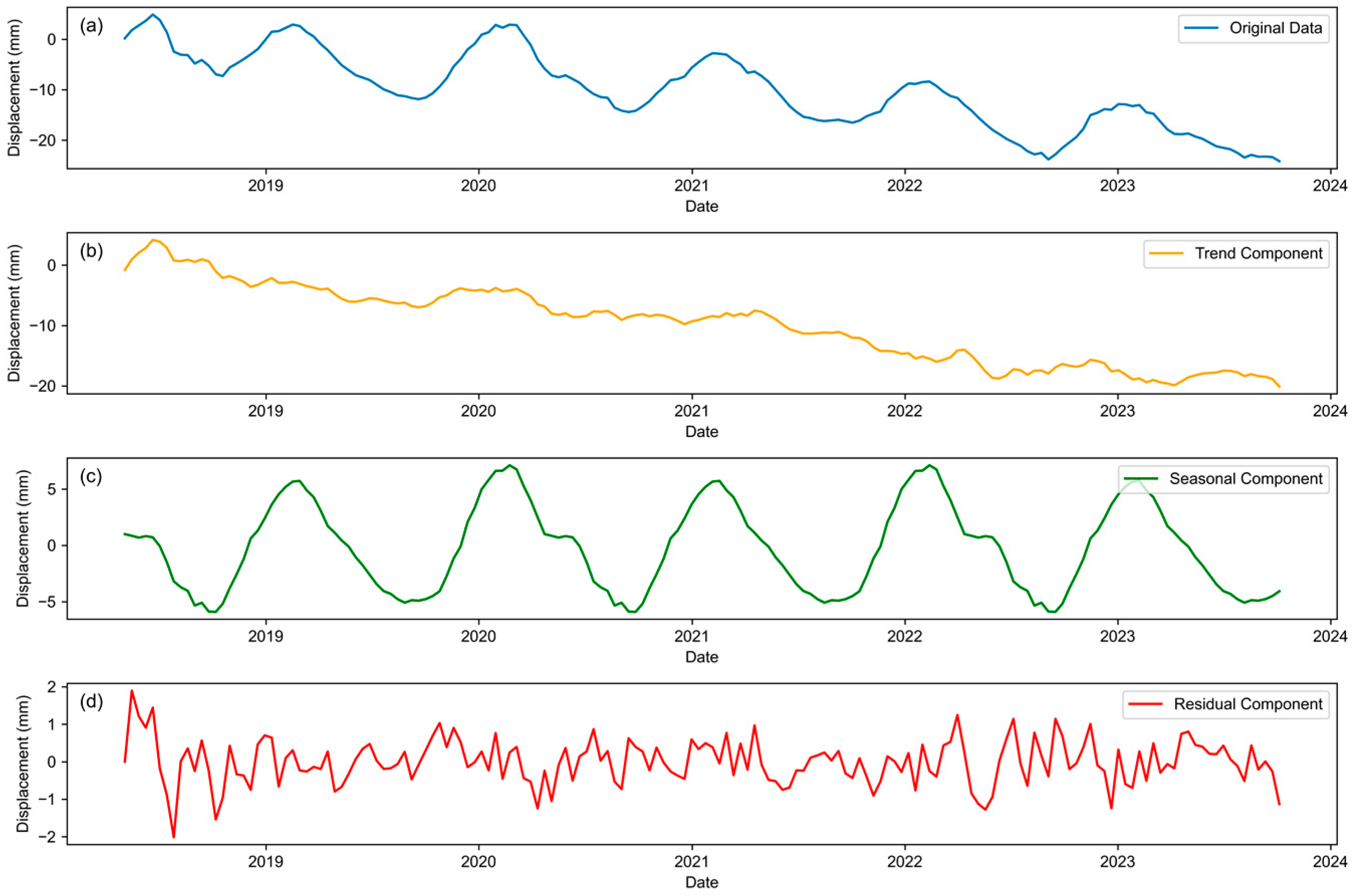
where represents the InSAR time-series deformation sequence of a measurement point in the study area, represents the trend component, represents the seasonal cycle component, represents the residual component, N is the number of measurement points, and is the serial number of a measurement point. The trend component represents the low-frequency and long-term changes in InSAR time-series deformation; the seasonal cycle component represents the periodic frequency changes in InSAR time-series deformation; the residual component represents the remaining values of the original InSAR time-series deformation after removing the trend and seasonal cycle components. For the InSAR time-series deformation dataset spanning from 3 May 2018 to 4 October 2023, with Sentinel-1A data’s revisit cycle of 12 days, the length of a yearly time series was about 30; hence, the Holt–Winters time-series decomposition seasonal periods parameter was set to 30. Note that for InSAR deformation data missing at 12-day intervals, bilinear interpolation was performed, resulting in a complete annual cycle of InSAR time-series data. Figure 5 displays the sequence characteristics of a point in the thaw slump area after Holt–Winters time-series decomposition, revealing that the point’s InSAR time-series data consisted of approximately 94.73% trend component, 31.60% cyclical component, and 4.40% residual component. The InSAR deformation data in this thaw slump area exhibited a declining trend, with seasonal deformation of permafrost on an annual cycle.
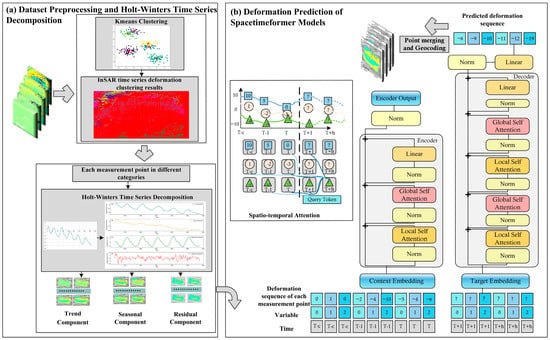
Figure 4.
The Spacetimeformer architecture for RTS deformation prediction. (a) Holt–Winters time-series decomposition; (b) model architecture.
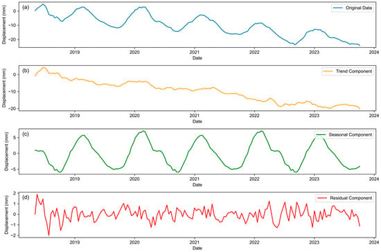
Figure 5.
Deformation time-series decomposition feature diagram. (a) InSAR time-series deformation; (b) trend component of displacement; (c) seasonal component of displacement; (d) residual component of displacement.
3.3.2. Deformation Prediction of Spacetimeformer Model
Figure 4b illustrates the single-layer encoder–decoder structure of the constructed Spacetimeformer network, which is based on transformer architecture [57]. This network utilizes a model to leverage the spatial relationships between different InSAR measurement points, thoroughly considering their temporal and spatial connections to learn additional useful dependencies. The Spacetimeformer network consists of an encoder and a decoder, each with five layers in this study. Both the encoder and decoder comprise embedding layers, attention layers, convolutional blocks, and normalization layers. The encoder’s embedding layer embeds each category’s time-series deformation sequences and timestamp sequences of all monitoring points, transforming them into a format suitable for the Spacetimeformer model. Similarly, the decoder’s embedding layer embeds feature inputs and target sequence inputs. Multiple attention layers in both encoder and decoder include global and local self-attention mechanisms. Global self-attention looks at the entire sequence to capture long-range dependencies, which is essential for understanding overall trends and patterns that span across the entire dataset. Local self-attention focuses on smaller segments of the input to capture fine-grained details and nuances, which is important for accurate local predictions and understanding localized events in the data. Convolutional blocks are crucial for extracting spatial features from input data, which is essential for tasks involving spatial relationships, such as predicting InSAR deformations where spatial context significantly influences outcomes. Normalization layers standardize the features for optimal processing.
The model exhibits capabilities for long-term time-series forecasting and dynamic spatial modeling, and it does not rely on hard-coded graphs. Typical deep learning time-series models group input values by time steps and learn patterns over time. However, when employing transformer-based models, traditional transformers primarily handle sequential information, which can lead to a neglect of spatial relationships among variables due to the “time” attention network. In contrast, graph neural networks and similar approaches explicitly model spatial relationships using graphs and share information across spatial and temporal layers alternately. The Spacetimeformer model incorporates both temporal and spatial dimensions using a customized transformer architecture and embeddings to implement spatiotemporal attention (see Figure 4b). This architecture allows the flattening of multivariate sequences so that each token at a given time step contains the value of a single variable, thereby enabling the modeling of both time series and spatial grids through the spatiotemporal attention mechanism, capturing spatial proximity and temporal dependencies. Thus, the Spacetimeformer learns the complete spatiotemporal patterns among all variables at each time step.
After completing the time-series decomposition of InSAR deformation data for all measurement points in each category, deformation datasets for each category were established. For the time-series deformation sequence of each category, past time series deformation data were used to predict the deformation data of h future time points. represents the timestamp value at time , and represents the deformation values of all InSAR measurement points at timestamp , i.e., , where is the number of measurement points in each category, and represents the deformation value of measurement point at timestamp . Given the timestamps and the deformation time series of all measurement points , the model predicts the deformation sequences of all measurement points at future time points . This model embeds the time series into a high-dimensional space, using zeros as placeholders for the unknown target sequence to achieve dimensional uniformity. The informer model further constructs an input sequence consisting of tokens through adding timestamps and corresponding vectors . This approach may cause the model to focus only on the temporal attributes of the time series, neglecting the spatial correlation of deformation data between different measurement points. The Spacetimeformer model addresses this issue by flattening each multidimensional vector into vectors with timestamps along the time dimension, transforming the input data into a spacetime sequence, thus generating a new embedded sequence .
3.3.3. Experimental Design
Model training, validation, and testing were conducted on a Dell T7920 workstation (hardware configuration: Intel Xeon Gold 6226R CPU, 128GB RAM, 2 RTX 4090 GPUs). Distributed training was executed on 2 RTX 4090 GPUs, utilizing Windows 11 as the operating system and the Pytorch deep learning framework as the runtime environment (Pytorch, an open-source platform developed by Facebook, operates on Python 3.8). The Spacetimeformer models were used to predict the trend, seasonal, and residual time-series deformation sequences.
The deformation pattern of permafrost exhibits periodic characteristics of freezing uplift and melting subsidence. Considering the local characteristics of the periodic components in the permafrost deformation pattern, to enable the Spacetimeformer models to learn the complete freeze–thaw cycle deformation pattern, we set the length of the training dataset’s time series to 100 (after interpolation, the total length of the InSAR time series deformation samples was 166, spanning from 3 May 2018 to 3 August 2021, covering three and a half freeze–thaw cycles). The length of the validation dataset was set to 33 (spanning from 15 August 2021 to 3 September 2022), and the test dataset was set to 33 (spanning from 15 September 2022 to 4 October 2023). For each dataset, the context_points parameter was set to 24, and the target_points parameter was set to 6, meaning the model used 24 previous time points for learning and prediction and predicted the deformation data for the next 6 time points, corresponding to 72 days of predicted InSAR time-series deformation data (with a 12-day interval). The weights of the Spacetimeformer neural network were iteratively updated using the AdamW optimizer [58], with a batch size of 16 and a training step length of 500. The initial learning rate was set to 1 × 10⁻¹⁰, and the base learning rate was set to 5 × 10⁻⁴. During inference, the trained Spacetimeformer model was used for estimating the time-series deformation prediction values for each pixel. Finally, the predicted time-series deformations for each category were geocoded, resulting in the generation of post-prediction time-series deformation maps.
The performance of the Spacetimeformer model was evaluated using root mean square error (RMSE), mean absolute error (MAE), mean absolute percentage error (MAPE), and symmetric mean absolute percentage error (SMAPE). The formulas are expressed as follows:
where represents the actual value of the i-th sample, represents the predicted value of the i-th sample, and n denotes the number of values.
4. Results and Analysis
4.1. InSAR Deformation Results
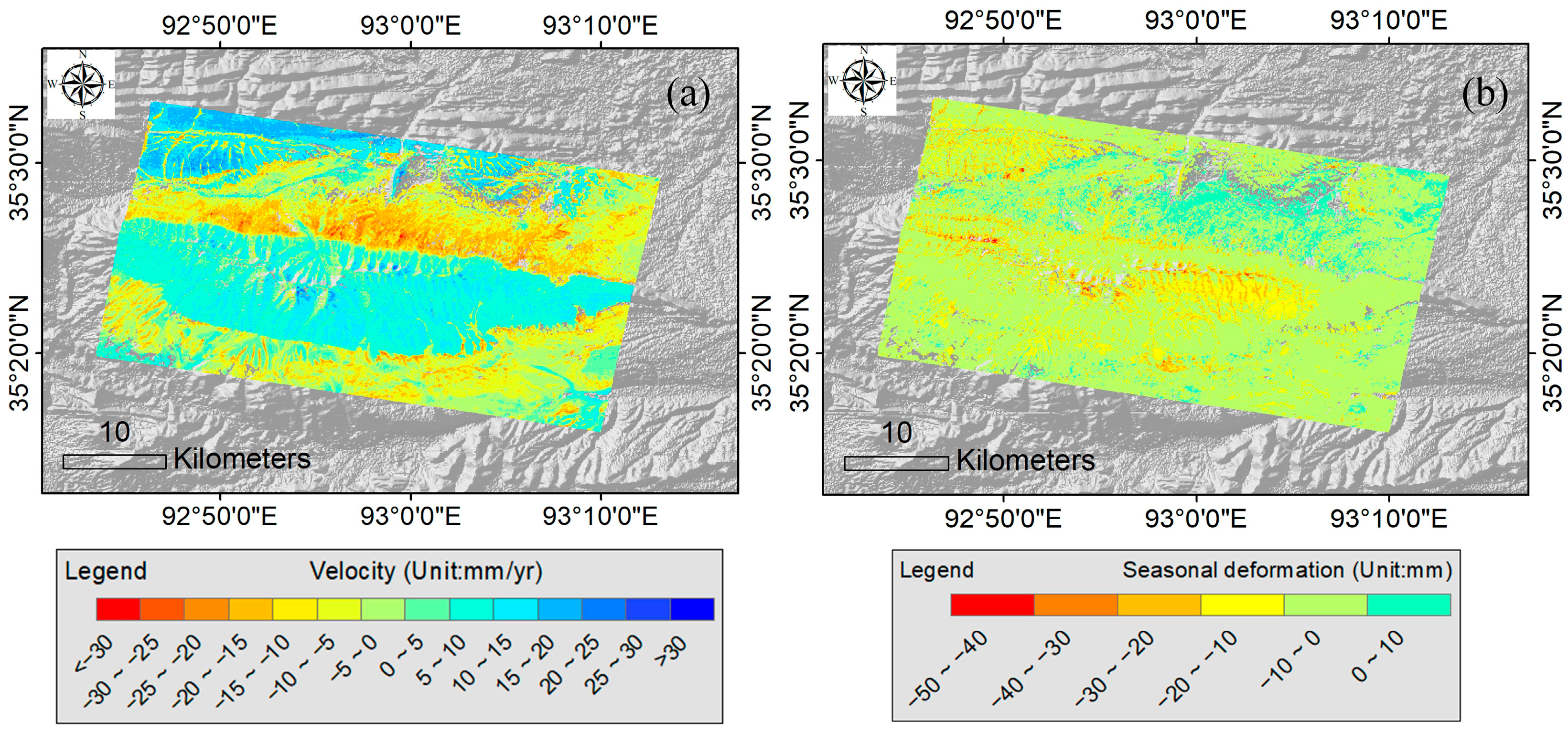
Figure 6 shows the surface deformation map of RTSs in the Chumar River Basin. Red colors represent deformation away from the satellite, while blue colors indicate deformation towards the LOS direction of the sensor. Figure 6a shows that the majority of the mountainous area had LOS deformation rates ranging from 5 to 15 mm/yr. These mountains consist of stable bedrock, lacking widespread permafrost and seasonally frozen ground, thereby resulting in lower deformation rates. In the foothills of the study area, the substantial presence of permafrost and seasonally frozen ground are primarily due to the cyclic freeze–thaw processes of the active layer and the degradation of permafrost. Additionally, high soil moisture content and abundant surface runoff contribute to higher LOS deformation rates and seasonal amplitudes. It is noteworthy that the upper left corner of the study area, with its extensive floodplain areas, was found to have high ground moisture content, resulting in deformation rates close to 10 to 25 mm/yr. The most significant subsidence was observed in the RTS areas, exhibiting deformation rates between −35 and 20 mm/year. In the study area’s northern part, long-term subsidence was notably evident, with LOS deformation rates reaching as high as 30 mm/year. This LOS deformation rate is closely related to the melting of ice-rich permafrost near the surface layer, reflecting the degradation trend of permafrost [59]. Additionally, Figure 6b shows significant seasonal deformation in the southern region of the study area, ranging from −50 mm to 10 mm, with the maximum seasonal deformation reaching about 50 mm. This seasonal deformation was caused by the freeze–thaw cycles of the active layer of the permafrost presenting periodic dynamic changes [11,13].
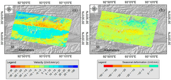
Figure 6.
Deformation results in the study area. (a) LOS deformation rate; (b) amplitude of seasonal deformation.
4.2. Extraction Results of Retrogressive Thaw Slumps
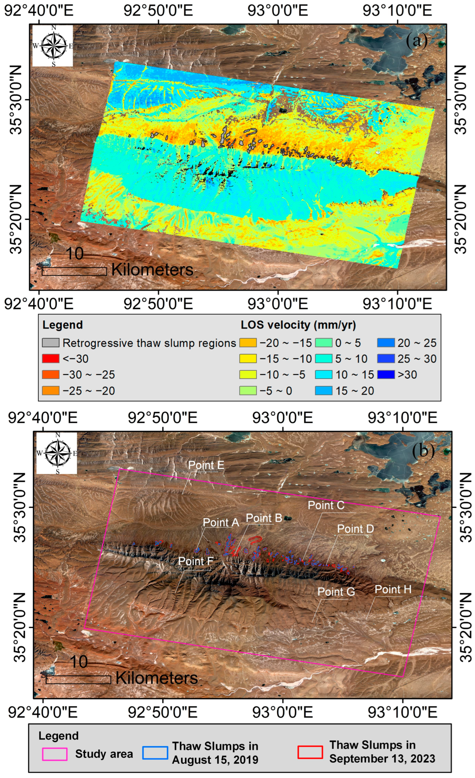
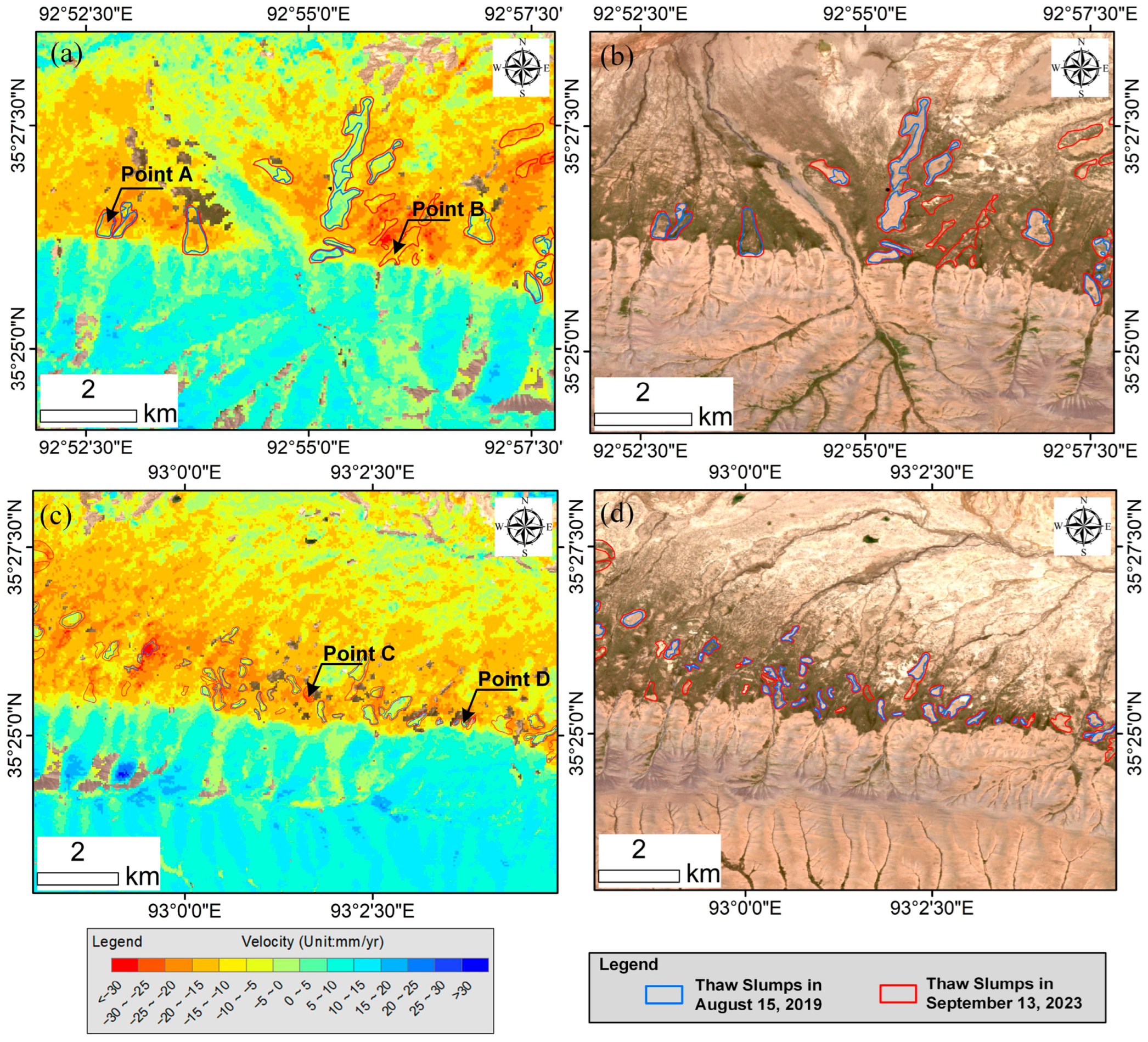
A thaw slump inventory for the study area was compiled based on the derived InSAR deformation maps and Sentinel-2 optical images, as depicted in Figure 7. Figure 7 shows the spatial distribution and deformation properties of the manually delineated thaw slumps. Combining remote sensing images with the distribution of RTSs, it was observed that most significant subsidence occurred within and around RTSs, with deformation rates ranging between −40 and 20 mm/year. Four representative points (Point A to Point D in Figure 7b) were selected from the RTSs areas on the LOS deformation rate map for further time-series investigation (as depicted in Figure 8). A significant number of thaw slumps in these inspection areas were included in the manually compiled thaw slump inventory. The boundaries of these thaw slumps in August 2019 (indicated in blue in Figure 7b) and September 2023 (shown in red in Figure 7b) were delineated. Among the existing 72 thaw slump areas, 64 exhibited an average deformation rate exceeding 10 mm/year, and 17 showed extreme deformation rates greater than 20 mm/year, with only a minority of areas remaining stable. Since RTSs occur in areas with gentle slopes, their change characteristics are more diverse than those of permafrost thawing. Additionally, it was observed that many deformations occurred outside the RTSs. These deformed areas do not necessarily indicate the occurrence of RTSs but are more likely to be areas prone to RTSs. Therefore, some regions with severe deformation do not have RTSs. Compared with 2019, the area of RTSs had increased by 3.98 km2 in 2023, and the number of such slumps had risen by 19. Notably, B and C were newly added retrogressive thaw slumps, while the areas of thaw slumps in regions A and D expanded by 49.29% and 51.40%, respectively. The InSAR observation results align with the aforementioned increase in thaw slump area and quantity, indicating that the Chumar River area is undergoing dynamic evolution of RTSs.

Figure 7.
Retrogressive thaw slumps in the Chumar River area. (a) InSAR-derived LOS velocity; (b) the retrogressive thaw slump areas mapped in 2019 and 2023.
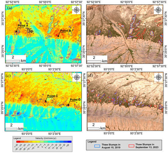
Figure 8.
Retrogressive thaw slump boundaries in 2019 (blue) and 2023 (red), manually extracted from Sentinel-2B images. (a,c) LOS velocity of Points A–D, (b,d) Sentinel-2B images of the areas of Points A–D.
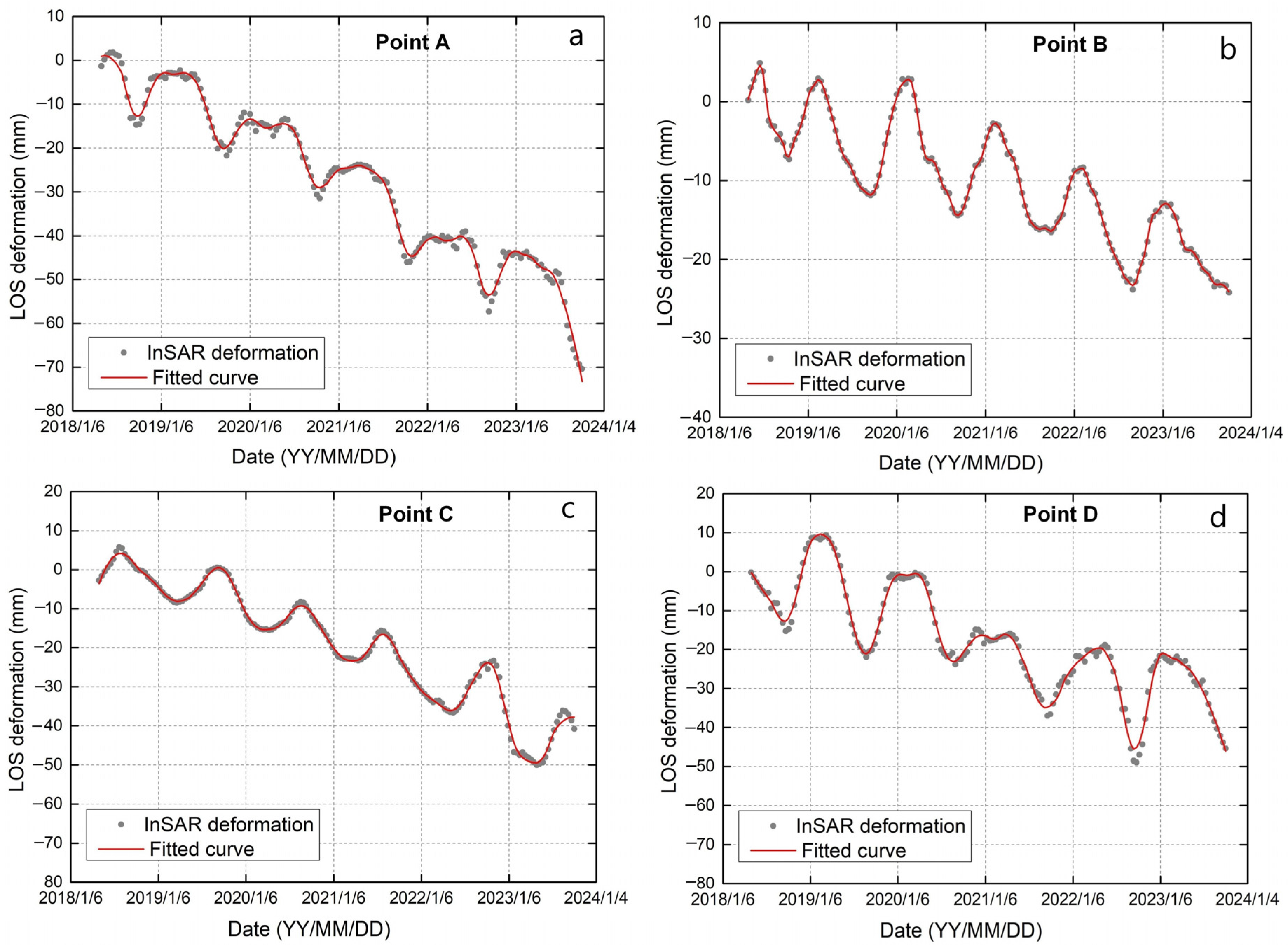
Figure 9 presents the time series and fitted curves for the locations of four points in RTS areas. The average LOS deformation rate and average cyclic amplitude for the RTS areas at these four points were calculated, as shown in Table 2. The deformation characteristics of these areas are marked by annually increasing LOS velocities and growing cyclic amplitudes, as seen from Figure 9. Notably, during the period from 2018 to 2023, the maximum subsidence observed in the Point A RTS area was 70.38 mm (Figure 9). Additionally, the maximum cyclic amplitude in the Point A RTS area was 36.08. The results indicate that each retrogressive thaw slump exhibited a distinct seasonal fluctuation trend, characterized by rising and sinking during the freeze–thaw seasons, respectively. Additionally, all four thaw slump areas showed a pronounced subsidence trend.
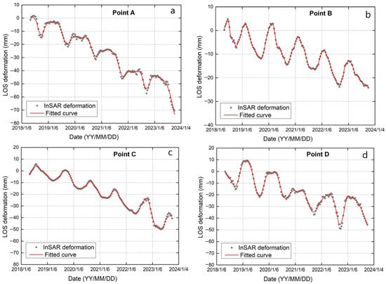
Figure 9.
Time-series deformation smoothed via the SG filter. (a) Point A; (b) Point B; (c) Point C; (d) Point D.

Table 2.
LOS velocity, periodic amplitude, and coherence calculated from the InSAR results for retrogressive thaw slumps in four sampled areas.
4.3. Time-Series Deformation Prediction Results
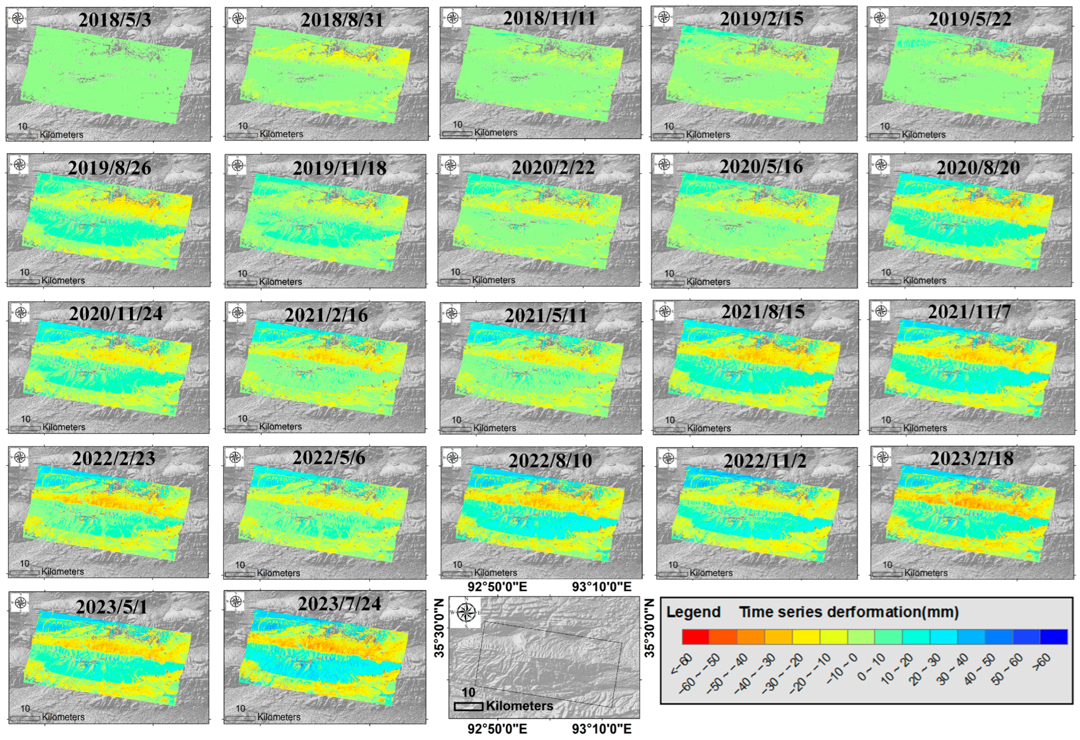
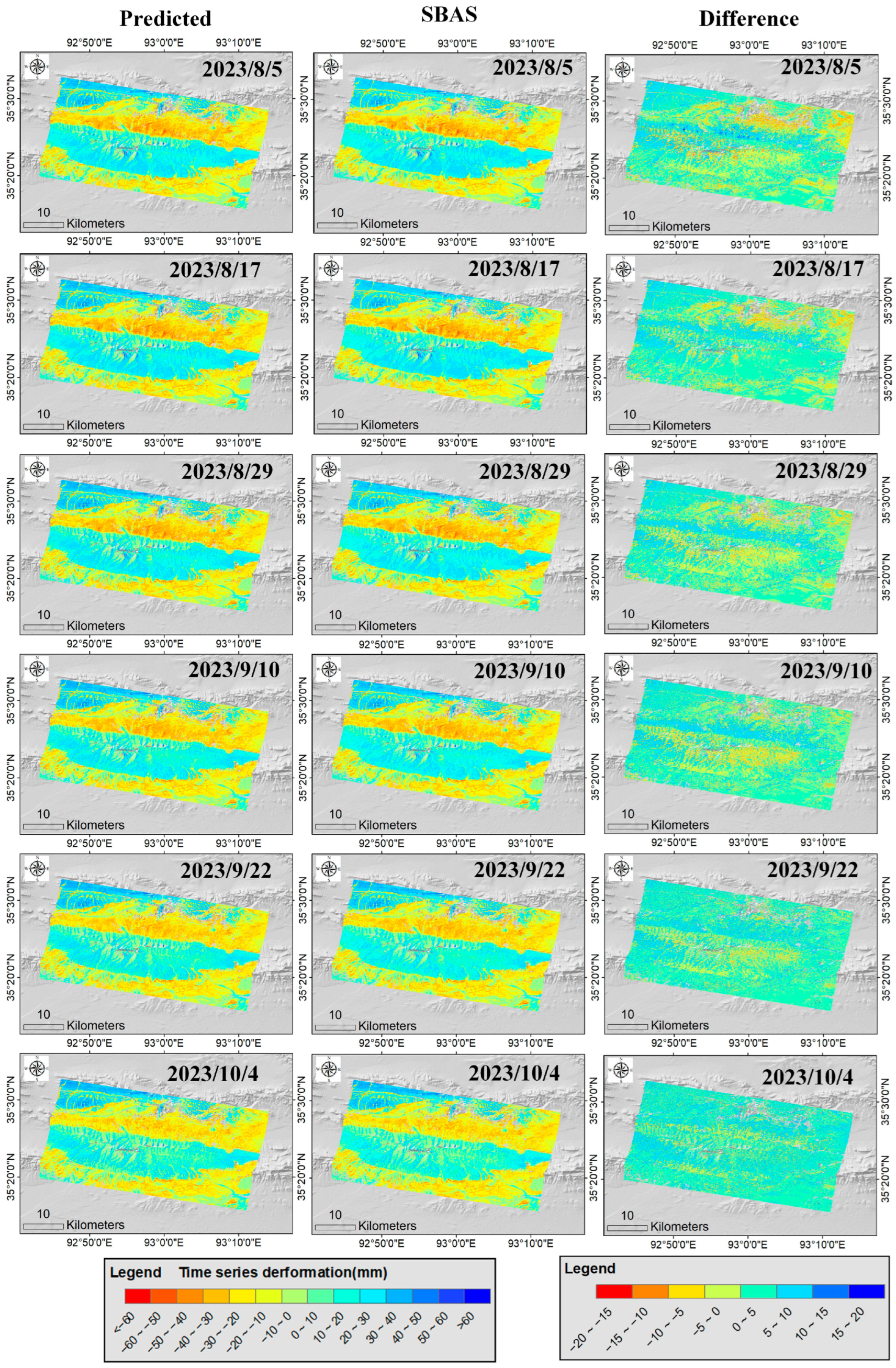
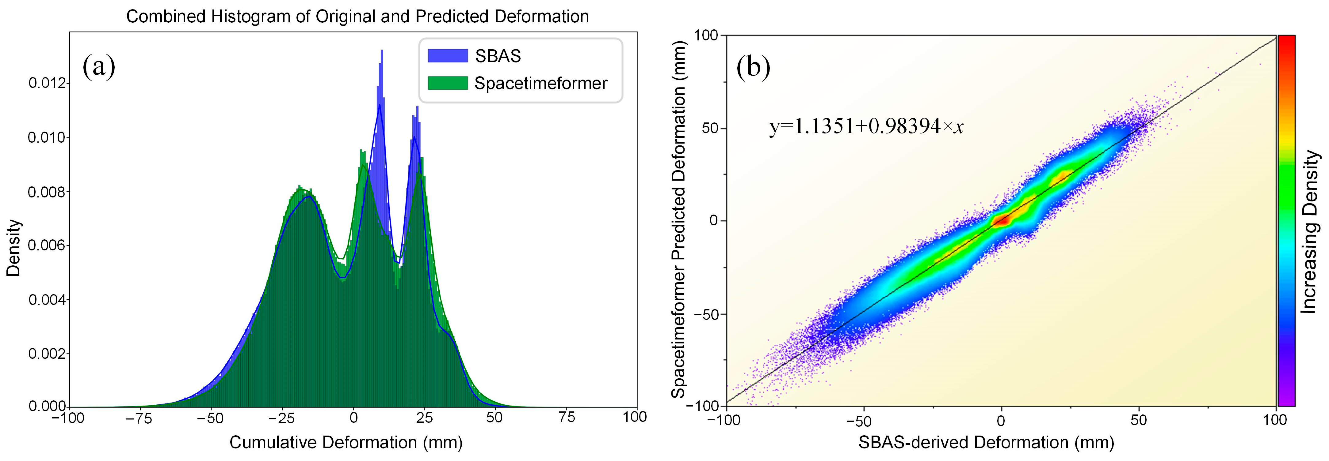
Figure 10 shows the time-series displacement from 3 May 2018 to 24 July 2023, a period of five years. Due to the freeze–thaw cycles of the permafrost, noticeable seasonal variations in the time-series deformation maps of the study are were observed. The comparison of time-series displacement between the Spacetimeformer model and the SBAS method from 5 August 2023 to 4 October 2023, as well as the residual map between the two methods, is shown in Figure 11. It was observed that the deformation map predicted by the model was essentially consistent with the deformation map monitored through the SBAS method during the same period. Although local high residuals were present in the time-series difference map, the overall prediction deviation remained within 20 mm, demonstrating the model’s effective predictive performance. To further illustrate the predictive performance of the Spacetimeformer model, Figure 12a presents a histogram comparing the monitored cumulative deformation with the predicted cumulative deformation, for 4 October 2023. There was no discernible difference between the cumulative deformation maps derived via the Spacetimeformer model and the SBAS method. The average values of the monitored and predicted deformation maps were −6 mm and −5 mm, respectively, with standard deviations of 45 mm and 42 mm, respectively. Figure 12b shows the point density distribution of the two results. The density distribution of predicted deformation was consistent with that of the Sentinel-1A data results, and the fitting result R2 was 0.95, confirming the validity of the predicted results.
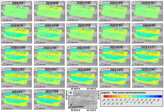
Figure 10.
Time-series deformation map of the study area (the time span is one quarter).

Figure 11.
The comparison of time-series displacement between the Spacetimeformer model and the SBAS method, as well as the residual map between the two methods, from 5 August 2023 to 4 October 2023. The first column displays the time-series deformation maps predicted with the model, the second column shows the time-series deformation map derived through the SBAS method, and the third column presents the difference maps of the time-series deformation between the two methods.
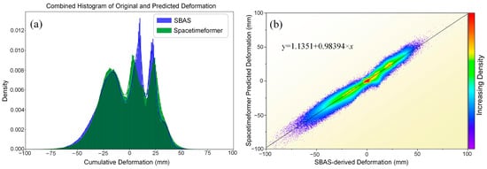
Figure 12.
Statistical results of the cumulative deformation on 4 October 2023. (a) Histograms of the cumulative deformation; (b) density distribution map of two results.
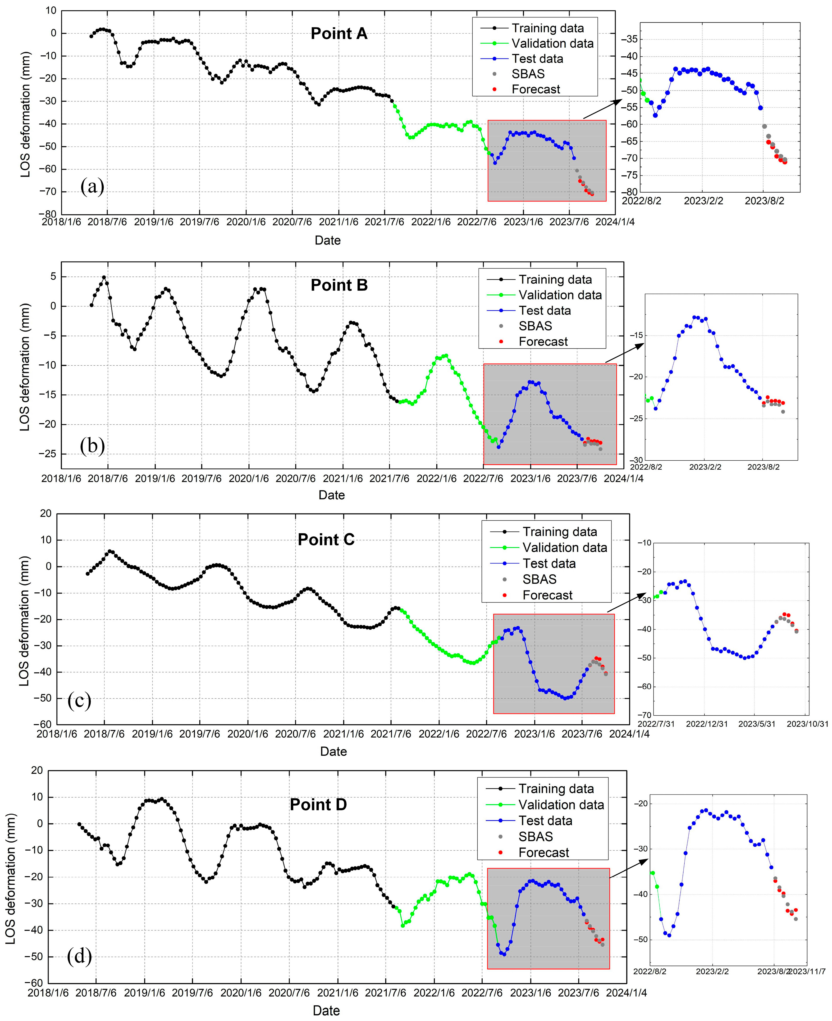
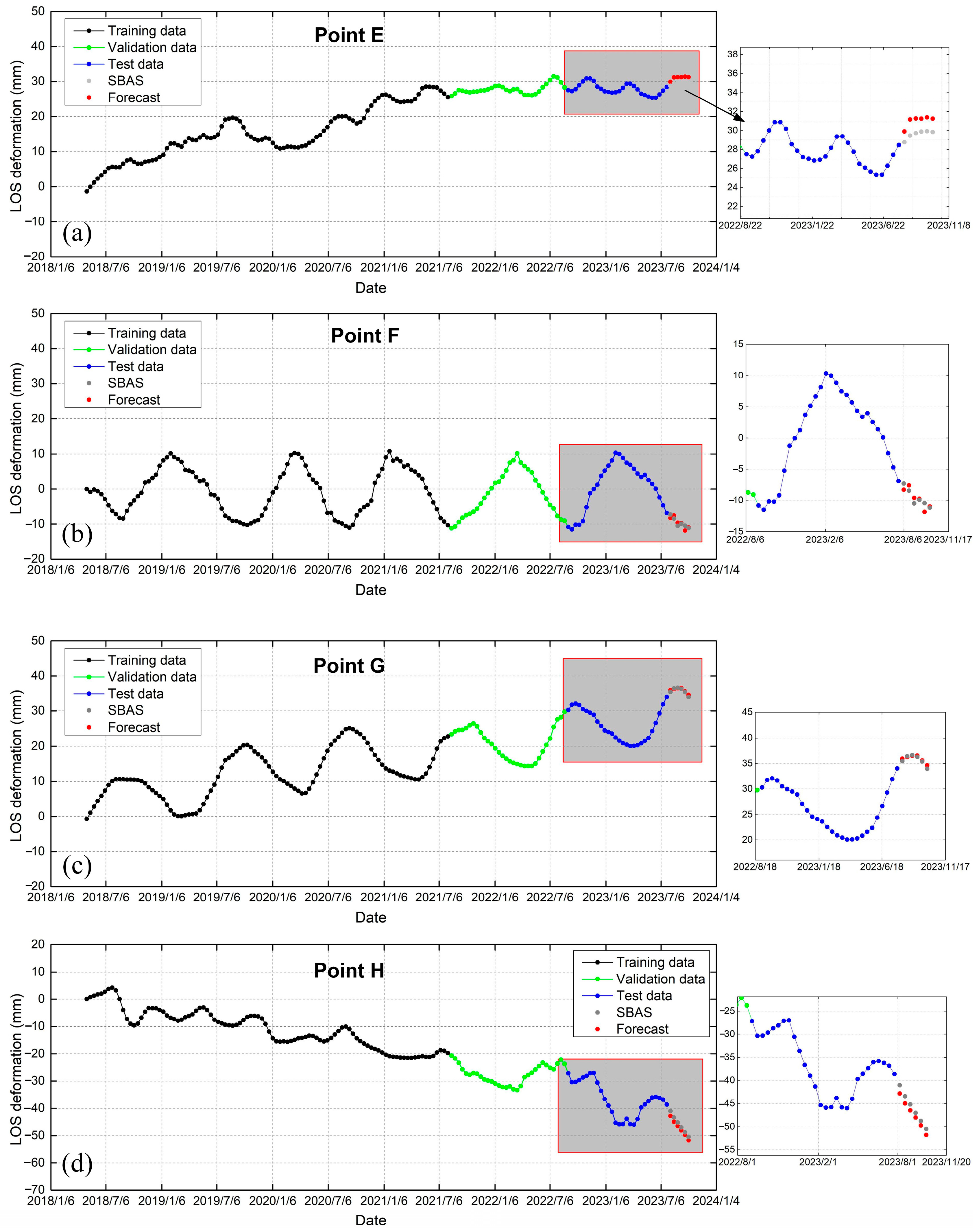
To further analyze the spatiotemporal variation trends of deformation in RTS areas, eight representative points were selected to display the predicted time-series results and analyze the deformation characteristics of the RTSs. Figure 13 and Figure 14 show the deformation prediction results of different deformation patterns based on the Spacetimeformer model. The blue curve represents the historical observed values of the data sample points, the gray curve indicates the actual label values of future trends for the sample points, and the red curve depicts the predictions of the Spacetimeformer network model. The prediction results follow the trend of historical permafrost deformation data. The comparison between predicted values and actual label values shows a high degree of alignment, demonstrating the effectiveness of the proposed method for predicting the deformation of RTSs. It is noteworthy that this model demonstrated better performance in predicting seasonal deformation patterns compared with long-term uplift and subsidence. When training, validating, and testing the Spacetimeformer model on eight different category datasets (A~H) corresponding to various data points, multiple evaluation metrics were employed, including RMS, MAE, MAPE, and SMAPE. Table 3 shows how these metrics comprehensively reflect the model’s performance across different category datasets, indicating a high level of prediction accuracy. Notably, the category containing data point D achieved the best results in the test dataset, with an RMSE of 1.249 mm and a MAE of 0.898 mm, demonstrating the model’s exceptional predictive capability in this category. The error metrics for the deformation trend predictions of the Spacetimeformer network model all met the requirements for deformation prediction, further demonstrating the method’s reliability from the perspective of real data experiments.
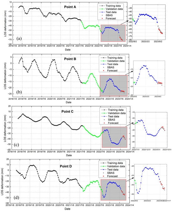
Figure 13.
The predicted InSAR time-series deformations at Point A (a), Point B (b), Point C (c), Point D (d).
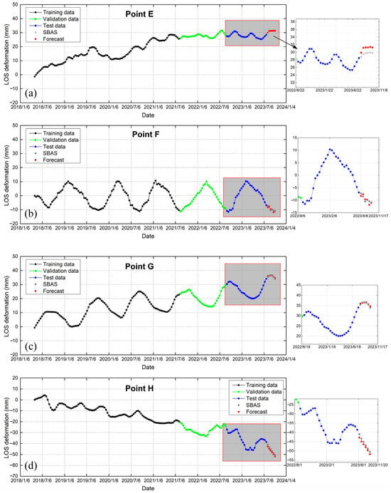
Figure 14.
The predicted InSAR time-series deformations at Point E (a), Point F (b), Point G (c), Point H (d).

Table 3.
Comparison of accuracy evaluation indexes of the Spacetimeformer model during training and testing at point scale.
5. Discussion
5.1. Discussion of Spacetimeformer Method in InSAR Time Series Deformation Prediction
InSAR deformation prediction is a time-series forecasting problem in the field of machine learning. Time-series forecasting typically relies on sequence-to-sequence methods, where past variable values within a k-step time range are used to predict future target values for h steps. Time-series forecasting plays a crucial role in areas like weather forecasting, traffic condition prediction, and financial forecasting. Predicting the deformation of RTSs using InSAR is a research-worthy domain. The vast historical deformation data and other time-series data can be utilized to predict future landslide deformation trends, providing quantitative assessment data for permafrost degradation in cold regions. With the advancement of artificial intelligence and deep learning, LSTM and transformer models have shown promising performance in InSAR deformation prediction. However, LSTM processes inputs sequentially as vectors, and its recursive structure limits capture long-term correlations in sequences. In contrast, the transformer model, with matrix inputs, eliminates the need for sequential input, allowing parallel processing of each token in the series. Hence, transformers have increasingly been applied in time-series forecasting tasks. Essentially, a transformer comprises a series of encoder and decoder layers with matrix inputs. Encoders use attention mechanisms to understand correlations between tokens, while decoders generate task-specific predictions using information from encoders. Current time-series prediction models still focus on point-by-point prediction, which is time-consuming and overlooks spatial correlations.
Traditional LSTM models and the latest transformer models mainly focus on the temporal correlations in InSAR deformation, neglecting the spatial relationships between InSAR deformation points. Yet, there often exist complex dynamic relationships between InSAR deformation points, such as similar influencing factors and deformation patterns in certain areas. Research on RTS InSAR deformation prediction considering spatiotemporal relationships is relatively scarce. In the Spacetimeformer model presented in this paper, direct connection paths exist between each token when data are processed through the attention layer, enabling the model to capture both temporal and spatial information simultaneously. This mechanism allows the Spacetimeformer to capture correlations between different variables at different time steps. The model enhances prediction accuracy by incorporating relative position information through positional embeddings and capturing periodic and aperiodic features of time with Time2Vec. The output of Time2Vec, combined with InSAR deformation data, is mapped onto the model through a forward propagation layer, forming the standard input sequence for the time-series prediction model. Additionally, the model differentiates deformation data at different time points through variable embeddings, flattening variable indicators along the time dimension and mapping them to the same dimension. Finally, variable values, time embeddings, and variable embeddings are combined to create the input sequence for the encoder, ensuring each token contains time, deformation, and other relevant information. The attention mechanism allows the model to accurately interpret temporal and spatial information embedded in the sequence, considering the mutual influence between different deformation measurement points. The Spacetimeformer model with spatiotemporal mechanisms used for InSAR deformation prediction in this paper captured relationships between different deformation measurement points at different times and enhanced predictive performance.
Currently, InSAR-based permafrost landslide deformation prediction is mostly based on time-series prediction at single measurement points. Due to limited computational capabilities of hardware devices, input data for a single training session should not be too large, necessitating preprocessing and time-series decomposition analysis of the training data. Thus, the method proposed in this paper is not suitable for large-scale InSAR deformation prediction. Future considerations could include predicting time-series deformation maps, where the input to the neural network is a time-series deformation map rather than single-point time-series deformation data. Although the Spacetimeformer network model has achieved good results in predicting deformation of retrogressive thaw slumps, there are still many unresolved issues in InSAR deformation prediction. For example, the prediction time span depends on the time span of the training data and cannot meet the need for short-term predictions beyond the InSAR time resolution. With the accumulation of more Sentinel-1 data in the future, it may be possible to predict long-term deformation using InSAR deformation data. Additionally, the method proposed in this paper inputs only InSAR deformation data; considering other factors influencing thaw slumps as supplementary input data is an area for improvement.
5.2. Comparing the Predictive Performance of the Spacetimeformer Model with Other Methods
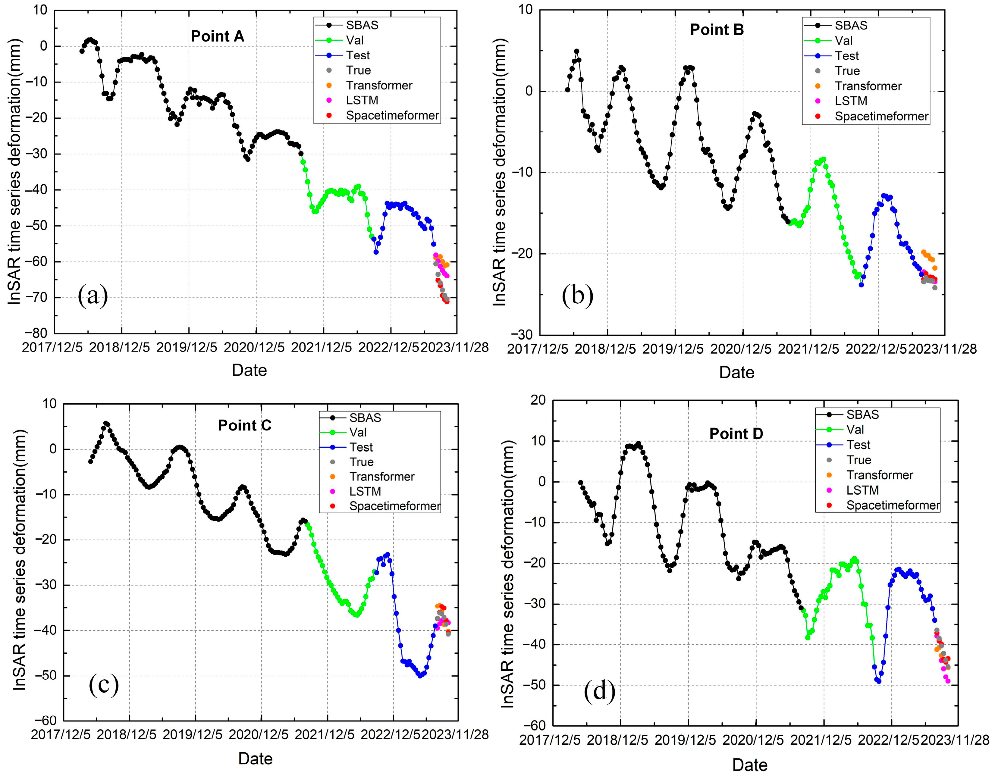
To evaluate the accuracy of the time-series deformation prediction proposed in this study, the LSTM, transformer, and Spacetimeformer methods were used to predict the displacement of points A to D in Figure 9, with a prediction window of six, significantly shorter than the signal period (1 year). The utilized LSTM model consisted of three LSTM layers, each with 256 hidden units, and employed sigmoid and tanh activation functions. The employed transformer model comprised three encoder layers and three decoder layers. It featured a model size of 512 dimensions and used the ReLU activation function, an eight-head multi-head attention mechanism, and a 2048-dimensional feed-forward network. Figure 15 shows the predicted results of different models. In all graphs, the gray line represents actual values, the red line represents the Spacetimeformer model, the orange line represents the transformer model, and the carmine line represents the LSTM model. Additionally, the errors between the predicted deformation and the actual deformation of all models were assessed using RMSE, MAE, MAPE, and SAMPE metrics, as detailed in Table 4, offering a comprehensive evaluation of the deformation prediction performance across different models.
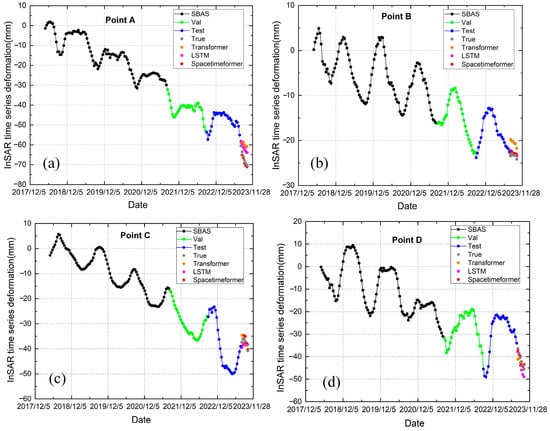
Figure 15.
InSAR time-series deformation curves based on LSTM, transformer, and Spacetimeformer models at Point A (a), Point B (b), Point C (c), Point D (d).

Table 4.
Comparison of accuracy evaluation indexes of different models.
It was evident that the Spacetimeformer model provided predictions closest to the actual InSAR deformation, and for the deformation prediction performance for all points, the Spacetimeformer model maintained robustness, as observed in Figure 15, with its predicted deformation closely matching the actual values. However, the predictive performance of the transformer model at point B was inferior to that of the traditional LSTM model. The transformer model primarily processes sequential information, utilizing a multi-head attention mechanism to capture long-distance dependencies within the sequence, and incorporates position encoding to inject positional information into the sequence. The Spacetimeformer model merges the characteristics of traditional transformer networks with innovative features such as spatiotemporal blocks and a novel self-attention mechanism. This allows it to model time series and spatial grids, capturing spatial proximity and temporal dependencies, thereby offering more precise predictions. Additionally, the Spacetimeformer model adopts the concept of spatiotemporal windows, enabling it to learn patterns at varying temporal and spatial granularities. Through integrating multi-scale attention mechanisms, it can effectively learn features on both global and local scales, adapting to various scale time-series prediction challenges.
Furthermore, the RMSE, MAE, MAPE, and RMSE metrics in Table 4 show that the Spacetimeformer model outperformed the other two methods in predicting all points. Table 4 shows that the Spacetimeformer model predicted future short-term InSAR time-series deformation with the smallest error, followed by the LSTM model, with the transformer model having the largest error. Most of the Spacetimeformer model’s predictions were close to the actual values, despite errors in the real data, which can be interpreted as natural fluctuations. The predictive performance of the transformer model was better than that of LSTM model at point C, but the transformer model had obvious deviations at some time points, indicating a poor smoothing process and reaffirming the effectiveness of the Spacetimeformer model with time and space concepts in InSAR deformation prediction tasks. Overall, the Spacetimeformer model continuously captured important trend changes in InSAR deformation prediction and provided relatively stable prediction results.
5.3. Combining InSAR Deformation RTSs for Detailed Explanation
Due to the high average altitude of the research area (above 4000 m), using only descending-track Sentinel-1 data to obtain deformation rates may not accurately capture all the dynamic changes of the Chumar River’s RTSs. Foreshortening effects may occur on steep slopes, leading to underestimations of the slopes’ deformation rates. An improvement could be to combine ascending-track data or use higher-resolution radar images to enhance the accuracy of RTS identification. In this study, to enhance the identification accuracy and reliability of RTSs, the threshold value of LOS deformation rate was set to 15 mm and was used as an auxiliary index of RTS area recognition. This threshold helped delineate potential thawing landslide areas. Further, time-series deformation data were used to filter out deformations unrelated to freeze–thaw degradation. Finally, multi-temporal Sentinel-2 optical remote sensing images were primarily utilized to map out the RTS areas.
The study area is located in the permafrost region of the QTP and experiences consistent permafrost conditions if the ice-rich upper layer does not thaw. The active layer undergoes precise, repetitive annual freeze–thaw cycles. In winter, soil moisture in the pores of the active layer freezes, causing the ground to rise; in summer, the pore ice melts into water, leading to ground subsidence. Therefore, their deformation patterns are characterized by periodic, seasonal subsidence and uplift. Typical RTSs are caused by the melting of ground ice on sloping terrain, resulting in irreversible subsidence due to the thawing of ice-rich permafrost. Initially, RTSs exhibit a stable deformation trend due to undisturbed vegetation cover on the surface. RTSs begin in summer with the melting of exposed ground ice at the headwall [60]. In the deformation sequence results, the headwall showed a pronounced melting trend. However, RTSs stabilized in autumn, as lower temperatures inhibited ice melting. After the onset of thaw slumping, the expansion of disturbed permafrost and the loss of protective vegetation increased the heat flux underground, accelerating permafrost thaw [61]. Additionally, the topographic depressions formed by RTSs led to winter snow accumulation, preventing soil heat from escaping into the cold atmosphere. In spring, snowmelt increased pore water pressure, further reducing slope stability. Thus, the deformation results of the RTSs represent a long-term linear subsidence trend and an increase in seasonal amplitude [7]. As shown in Figure 14, the deformation predicted using the Spacetimeformer model accurately forecasted the periodic deformation patterns of permafrost and the degradation trends of RTSs, providing quantitative data for studying the changing deformation trends of RTSs and permafrost degradation.
6. Conclusions
In this study, the Chumar River Basin was selected as the test area. A displacement prediction method for InSAR time series based on the Spacetimeformer is proposed; the study highlights the outstanding performance of the Spacetimeformer model in short-term deformation prediction for degradative thaw slumps. The method shows great potential for application in deformation prediction in areas of RTSs. Based on the research results, the following conclusions are drawn:
For the degradative melting slumps in the permafrost regions, three types of products were derived: ground LOS velocity maps, periodic amplitude maps, and melting slump distribution maps. The SBAS results of Sentinel-1 remote sensing images from 2018 to 2023 showed that in most areas, the range of LOS velocity change was −10 mm/year to 10 mm/year, and the seasonal displacement range was −60 mm to 10 mm. Through combining the deformation results derived from InSAR and optical images from Sentinel-2, we identified 72 degradative melting slump areas in the study area. Compared with normal permafrost degradation, the displacement speed of the degradative melting slump permafrost zones was faster (−35 to 20 mm/year). Compared with 2019, the area of RTSs increased by 3.98 km2 in 2023, and the number of such slumps rose by 19.
The network based on Spacetimeformer can accurately simulate the seasonal deformation signals of degradative melting slumps and predict the degradation trend of permafrost. This displacement prediction method was shown to have high accuracy, with RMSE, MAE, MAPE and SMAPE of 1.249 mm, 0.898 mm, 0.408 and 0.223, respectively, for displacement points predicted three months later. The prediction error of the predicted time series deformation map compared with the InSAR-inverted time-series deformation map was within 20 mm. Additionally, the density distribution of the predicted deformation aligned consistently with that derived from Sentinel-1A data results, achieving a fitting result R2 of 0.95. Compared with other deep learning methods, the Spacetimeformer model with its spatiotemporal concept demonstrated better deformation prediction performance than the transformer and LSTM models. The Spacetimeformer model can continuously capture important trend changes in deformation prediction and provide relatively stable prediction results.
In the future, more Sentinel-1 SAR data will be incorporated into the Spacetimeformer network, and factors influencing degradative melting slumps such as air temperature data and precipitation data will also be considered for inclusion in the Spacetimeformer model to improve prediction accuracy. In addition, the fusion of InSAR data with other high-temporal-resolution data for predicting RTS deformation is also a valuable direction.
Author Contributions
Conceptualization, X.F. and J.W.; methodology, J.W. and X.Z.; software, J.W., Z.Z. and X.Z.; validation, J.W., W.N. and Y.Q.; formal analysis, W.N., Y.Q. and N.Z.; investigation, N.Z.; resources, X.F.; data curation, Z.Z.; writing—original draft preparation, J.W.; writing—review and editing, X.F.; visualization, Z.Z.; supervision, X.F.; project administration, X.F.; funding acquisition, X.F. and X.Z. All authors have read and agreed to the published version of the manuscript.
Funding
This research was jointly funded by and the National Natural Science Foundation of China, grant number 4207133, the National Nonprofit Fundamental Research Grant of China, Institute of Geology, China Earthquake Administration, grant number ICCEA2106, and the National Natural Science Foundation Youth Foundation of China, grant number 4230012403.
Data Availability Statement
Sentinel-1 data were provided by the European Space Agency (ESA) and available from the Alaska Satellite Facility (ASF) (https://vertex.daac.asf.alaska.edu (accessed on 19 May 2024)). SRTM DEM data are available at https://srtm.csi.cgiar.org/srtmdata/ (accessed on 19 May 2024). ERA5- daily air temperatures are available at https://cds.climate.copernicus.eu/cdsapp#!/home (accessed on 19 May 2024).
Acknowledgments
The authors would like to thank the EU Copernicus Program for providing the Sentinel-1A SAR data, and NASA and CGIAR-CSI for providing SRTM DEM data. Special thanks go to the Climate Data Store (CDS) for providing the fifth-generation ECMWF reanalysis products (ERA5). Chao Wang, Hong Zhang of Aerospace Information Research Institute, Chinese Academy of Sciences, and Zhengjia Zhang of China University of Geosciences are acknowledged for helpful discussions.
Conflicts of Interest
The authors declare no conflicts of interest.
References
- Zou, D.; Zhao, L.; Sheng, Y.; Chen, J.; Hu, G.; Wu, T.; Wu, J.; Xie, C.; Wu, X.; Pang, Q.; et al. A New Map of Permafrost Distribution on the Tibetan Plateau. Cryosphere 2017, 11, 2527–2542. [Google Scholar] [CrossRef]
- Ran, Y.; Li, X.; Cheng, G. Climate Warming Has Led to the Degradation of Permafrost Stability in the Past Half Century over the Qinghai-Tibet Plateau; Frozen Ground. Cryosphere Discuss. 2017, 12, 1–30. [Google Scholar] [CrossRef]
- Yang, M.; Nelson, F.E.; Shiklomanov, N.I.; Guo, D.; Wan, G. Permafrost Degradation and Its Environmental Effects on the Tibetan Plateau: A Review of Recent Research. Earth-Sci. Rev. 2010, 103, 31–44. [Google Scholar] [CrossRef]
- Luo, J.; Niu, F.; Lin, Z.; Liu, M.; Yin, G. Recent Acceleration of Thaw Slumping in Permafrost Terrain of Qinghai-Tibet Plateau: An Example from the Beiluhe Region. Geomorphology 2019, 341, 79–85. [Google Scholar] [CrossRef]
- Olefeldt, D.; Goswami, S.; Grosse, G.; Hayes, D.; Hugelius, G.; Kuhry, P.; McGuire, A.D.; Romanovsky, V.E.; Sannel, A.B.K.; Schuur, E.A.G.; et al. Circumpolar Distribution and Carbon Storage of Thermokarst Landscapes. Nat. Commun. 2016, 7, 13043. [Google Scholar] [CrossRef]
- Turetsky, M.R.; Abbott, B.W.; Jones, M.C.; Walter Anthony, K.; Olefeldt, D.; Schuur, E.A.G.; Koven, C.; McGuire, A.D.; Grosse, G.; Kuhry, P.; et al. Permafrost Collapse Is Accelerating Carbon Release. Nature 2019, 569, 32–34. [Google Scholar] [CrossRef]
- Jiao, Z.; Xu, Z.; Guo, R.; Zhou, Z.; Jiang, L. Potential of Multi-Temporal InSAR for Detecting Retrogressive Thaw Slumps: A Case of the Beiluhe Region of the Tibetan Plateau. Int. J. Disaster Risk Sci. 2023, 14, 523–538. [Google Scholar] [CrossRef]
- Zhang, Z.; Lin, H.; Wang, M.; Liu, X.; Chen, Q.; Wang, C.; Zhang, H. A Review of Satellite Synthetic Aperture Radar Interferometry Applications in Permafrost Regions: Current Status, Challenges, and Trends. IEEE Geosci. Remote Sens. Mag. 2022, 10, 93–114. [Google Scholar] [CrossRef]
- Ferretti, A.; Prati, C.; Rocca, F. Permanent Scatterers in SAR Interferometry. IEEE Trans. Geosci. Remote Sens. 2001, 39, 8–20. [Google Scholar] [CrossRef]
- Berardino, P.; Fornaro, G.; Lanari, R.; Sansosti, E. A New Algorithm for Surface Deformation Monitoring Based on Small Baseline Differential SAR Interferograms. IEEE Trans. Geosci. Remote Sens. 2002, 40, 2375–2383. [Google Scholar] [CrossRef]
- Zhang, X.; Zhang, H.; Wang, C.; Tang, Y.; Zhang, B.; Wu, F.; Wang, J.; Zhang, Z. Time-Series InSAR Monitoring of Permafrost Freeze-Thaw Seasonal Displacement over Qinghai–Tibetan Plateau Using Sentinel-1 Data. Remote Sens. 2019, 11, 1000. [Google Scholar] [CrossRef]
- Wang, L.; Marzahn, P.; Bernier, M.; Ludwig, R. Sentinel-1 InSAR Measurements of Deformation over Discontinuous Permafrost Terrain, Northern Quebec, Canada. Remote Sens. Environ. 2020, 248, 111965. [Google Scholar] [CrossRef]
- Wang, J.; Wang, C.; Zhang, H.; Tang, Y.; Duan, W.; Dong, L. Freeze-Thaw Deformation Cycles and Temporal-Spatial Distribution of Permafrost along the Qinghai-Tibet Railway Using Multitrack InSAR Processing. Remote Sens. 2021, 13, 4744. [Google Scholar] [CrossRef]
- Lu, P.; Han, J.; Yi, Y.; Hao, T.; Zhou, F.; Meng, X.; Zhang, Y.; Li, R. MT-InSAR Unveils Dynamic Permafrost Disturbances in Hoh Xil (Kekexili) on the Tibetan Plateau Hinterland. IEEE Trans. Geosci. Remote Sens. 2023, 61, 1–16. [Google Scholar] [CrossRef]
- Wang, Y.; Sun, Z.; Sun, Y. Effects of a Thaw Slump on Active Layer in Permafrost Regions with the Comparison of Effects of Thermokarst Lakes on the Qinghai–Tibet Plateau, China. Geoderma 2018, 314, 47–57. [Google Scholar] [CrossRef]
- Zhang, X.; Zhang, H.; Wang, C.; Tang, Y.; Zhang, B.; Wu, F.; Wang, J.; Zhang, Z. Active Layer Thickness Retrieval Over the Qinghai-Tibet Plateau Using Sentinel-1 Multitemporal InSAR Monitored Permafrost Subsidence and Temporal-Spatial Multilayer Soil Moisture Data. IEEE Access 2020, 8, 84336–84351. [Google Scholar] [CrossRef]
- Mudelsee, M. Trend Analysis of Climate Time Series: A Review of Methods. Earth-Sci. Rev. 2019, 190, 310–322. [Google Scholar] [CrossRef]
- Stoffer, D.S.; Ombao, H. Editorial: Special Issue on Time Series Analysis in the Biological Sciences. J. Time Ser. Anal. 2012, 33, 701–703. [Google Scholar] [CrossRef]
- Topol, E.J. High-Performance Medicine: The Convergence of Human and Artificial Intelligence. Nat. Med. 2019, 25, 44–56. [Google Scholar] [CrossRef]
- Lim, B.; Zohren, S. Time Series Forecasting with Deep Learning: A Survey. Philos. Trans. R. Soc. A 2020, 379, 20200209. [Google Scholar] [CrossRef]
- Adhikari, R.; Agrawal, R.K. An Introductory Study on Time Series Modeling and Forecasting. arXiv 2013, arXiv:1302.6613. [Google Scholar]
- Bartholomew, D.J.; Box, G.E.P.; Jenkins, G.M. Time Series Analysis Forecasting and Control. Oper. Res. Q. 1971, 22, 199. [Google Scholar] [CrossRef]
- Winters, P.R. Forecasting Sales by Exponentially Weighted Moving Averages. Manag. Sci. 1960, 6, 324–342. [Google Scholar] [CrossRef]
- Harvey, A.C. Forecasting, Structural Time Series Models and the Kalman Filter; Cambridge University Press: Cambridge, UK, 1990. [Google Scholar]
- Deng, Z.; Ke, Y.; Gong, H.; Li, X.; Li, Z. Land Subsidence Prediction in Beijing Based on PS-InSAR Technique and Improved Grey-Markov Model. GIScience Remote Sens. 2017, 54, 797–818. [Google Scholar] [CrossRef]
- Kim, S.; Wdowinski, S.; Dixon, T.H.; Amelung, F.; Kim, J.W.; Won, J. Measurements and Predictions of Subsidence Induced by Soil Consolidation Using Persistent Scatterer InSAR and a Hyperbolic Model. Geophys. Res. Lett. 2010, 37, 2009GL041644. [Google Scholar] [CrossRef]
- Aoqing, G.U.O.; Jun, H.U.; Wanji, Z.; Rong, G.U.I.; Zhigui, D.U.; Wu, Z.H.U.; Lehe, H.E. N-BEATS Deep Learning Method for Landslide Deformation Monitoring and Prediction Based on InSAR: A Case Study of Xinpu Landslide. Acta Geod. Et Cartogr. Sin. 2022, 51, 2171. [Google Scholar] [CrossRef]
- Ding, Q.; Shao, Z.; Huang, X.; Altan, O.; Zhuang, Q.; Hu, B. Monitoring, Analyzing and Predicting Urban Surface Subsidence: A Case Study of Wuhan City, China. Int. J. Appl. Earth Obs. Geoinf. 2021, 102, 102422. [Google Scholar] [CrossRef]
- Ahmed, N.K.; Atiya, A.F.; Gayar, N.E.; El-Shishiny, H. An Empirical Comparison of Machine Learning Models for Time Series Forecasting. Econom. Rev. 2010, 29, 594–621. [Google Scholar] [CrossRef]
- Antonova, S.; Sudhaus, H.; Strozzi, T.; Zwieback, S.; Kääb, A.; Heim, B.; Langer, M.; Bornemann, N.; Boike, J. Thaw Subsidence of a Yedoma Landscape in Northern Siberia, Measured In Situ and Estimated from TerraSAR-X Interferometry. Remote Sens. 2018, 10, 494. [Google Scholar] [CrossRef]
- Ma, P.; Zhang, F.; Lin, H. Prediction of InSAR Time-Series Deformation Using Deep Convolutional Neural Networks. Remote Sens. Lett. 2020, 11, 137–145. [Google Scholar] [CrossRef]
- Nukala, V.H.; Nayak, M.; Gubbi, J.; Purushothaman, B. Multi-Scale Attention Guided Recurrent Neural Network for Deformation Map Forecasting. In Proceedings of the Image and Signal Processing for Remote Sensing XXVII, Online, 13–17 September 2021; SPIE: Bellingham, WI, USA, 2021; Volume 11862, pp. 154–159. [Google Scholar]
- Chen, Y.; He, Y.; Zhang, L.; Chen, Y.; Pu, H.; Chen, B.; Gao, L. Prediction of InSAR Deformation Time-Series Using a Long Short-Term Memory Neural Network. Int. J. Remote Sens. 2021, 42, 6919–6942. [Google Scholar] [CrossRef]
- Hill, P.; Biggs, J.; Ponce-López, V.; Bull, D. Time-Series Prediction Approaches to Forecasting Deformation in Sentinel-1 InSAR Data. JGR Solid Earth 2021, 126, e2020JB020176. [Google Scholar] [CrossRef]
- Bao, X.; Zhang, R.; Shama, A.; Li, S.; Xie, L.; Lv, J.; Fu, Y.; Wu, R.; Liu, G. Ground Deformation Pattern Analysis and Evolution Prediction of Shanghai Pudong International Airport Based on PSI Long Time Series Observations. Remote Sens. 2022, 14, 610. [Google Scholar] [CrossRef]
- Wang, J.; Li, C.; Li, L.; Huang, Z.; Wang, C.; Zhang, H.; Zhang, Z. InSAR Time-Series Deformation Forecasting Surrounding Salt Lake Using Deep Transformer Models. Sci. Total Environ. 2023, 858, 159744. [Google Scholar] [CrossRef] [PubMed]
- Yao, S.; He, Y.; Zhang, L.; Yang, W.; Chen, Y.; Sun, Q.; Zhao, Z.; Cao, S. A ConvLSTM Neural Network Model for Spatiotemporal Prediction of Mining Area Surface Deformation Based on SBAS-InSAR Monitoring Data. IEEE Trans. Geosci. Remote Sens. 2023, 61, 1–22. [Google Scholar] [CrossRef]
- He, Y.; Yao, S.; Chen, Y.; Yan, H.; Zhang, L. Spatio-temporal prediction of time-series InSAR Land subsidence based on ConvLSTM neural network. Geomat. Inf. Sci. Wuhan Univ. 2023, 1–21. [Google Scholar] [CrossRef]
- Xia, L.; Yang, Q.; Li, Z.; Wu, Y.; Feng, Z. The Effect of the Qinghai-Tibet Railway on the Migration of Tibetan Antelope Pantholops Hodgsonii in Hoh-Xil National Nature Reserve, China. Oryx 2007, 41, 352–357. [Google Scholar] [CrossRef]
- Yao, X.; Li, L.; Zhao, J.; Sun, M.; Li, J.; Gong, P.; An, L. Spatial-Temporal Variations of Lake Ice Phenology in the Hoh Xil Region from 2000 to 2011. J. Geogr. Sci. 2016, 26, 70–82. [Google Scholar] [CrossRef]
- Yang, Y.; Wu, Q.; Zhang, P.; Jiang, G. Stable Isotopic Evolutions of Ground Ice in Permafrost of the Hoh Xil Regions on the Qinghai-Tibet Plateau. Quat. Int. 2017, 444, 182–190. [Google Scholar] [CrossRef]
- Zhao, L.; Zou, D.; Hu, G.; Du, E.; Pang, Q.; Xiao, Y.; Li, R.; Sheng, Y.; Wu, X.; Sun, Z.; et al. Changing Climate and the Permafrost Environment on the Qinghai–Tibet (Xizang) Plateau. Permafr. Periglac. Process. 2020, 31, 396–405. [Google Scholar] [CrossRef]
- Lanari, R.; Casu, F.; Manzo, M.; Zeni, G.; Berardino, P.; Manunta, M.; Pepe, A. An Overview of the Small BAseline Subset Algorithm: A DInSAR Technique for Surface Deformation Analysis. In Deformation and Gravity Change: Indicators of Isostasy, Tectonics, Volcanism, and Climate Change; Wolf, D., Fernández, J., Eds.; Pageoph Topical Volumes; Birkhäuser Basel: Basel, Switzerland, 2007; pp. 637–661. ISBN 978-3-7643-8416-6. [Google Scholar]
- Hersbach, H.; Bell, B.; Berrisford, P.; Hirahara, S.; Horányi, A.; Muñoz-Sabater, J.; Nicolas, J.; Peubey, C.; Radu, R.; Schepers, D.; et al. The ERA5 Global Reanalysis. Quart. J. R. Meteoro. Soc. 2020, 146, 1999–2049. [Google Scholar] [CrossRef]
- Savitzky, A.; Golay, M.J.E. Smoothing and Differentiation of Data by Simplified Least Squares Procedures. Available online: https://pubs.acs.org/doi/pdf/10.1021/ac60214a047 (accessed on 21 December 2023).
- Ahmed, M.; Seraj, R.; Islam, S.M.S. The K-Means Algorithm: A Comprehensive Survey and Performance Evaluation. Electronics 2020, 9, 1295. [Google Scholar] [CrossRef]
- Chatfield, C. The Holt-Winters Forecasting Procedure. J. R. Stat. Soc. Ser. C (Appl. Stat.) 1978, 27, 264–279. [Google Scholar] [CrossRef]
- Prats-Iraola, P.; Scheiber, R.; Marotti, L.; Wollstadt, S.; Reigber, A. TOPS Interferometry with TerraSAR-X. IEEE Trans. Geosci. Remote Sens. 2012, 50, 3179–3188. [Google Scholar] [CrossRef]
- Yague-Martinez, N.; Prats-Iraola, P.; Rodriguez Gonzalez, F.; Brcic, R.; Shau, R.; Geudtner, D.; Eineder, M.; Bamler, R. Interferometric Processing of Sentinel-1 TOPS Data. IEEE Trans. Geosci. Remote Sens. 2016, 54, 2220–2234. [Google Scholar] [CrossRef]
- Xu, X.; Sandwell, D.T.; Tymofyeyeva, E.; Gonzalez-Ortega, A.; Tong, X. Tectonic and Anthropogenic Deformation at the Cerro Prieto Geothermal Step-over Revealed by Sentinel-1A InSAR. IEEE Trans. Geosci. Remote Sens. 2017, 55, 5284–5292. [Google Scholar] [CrossRef]
- Goldstein, R.M.; Werner, C.L. Radar Interferogram Filtering for Geophysical Applications. Geophys. Res. Lett. 1998, 25, 4035–4038. [Google Scholar] [CrossRef]
- Pepe, A.; Lanari, R. On the Extension of the Minimum Cost Flow Algorithm for Phase Unwrapping of Multitemporal Differential SAR Interferograms. IEEE Trans. Geosci. Remote Sens. 2006, 44, 2374–2383. [Google Scholar] [CrossRef]
- Chen, J.; Liu, L.; Zhang, T.; Cao, B.; Lin, H. Using Persistent Scatterer Interferometry to Map and Quantify Permafrost Thaw Subsidence: A Case Study of Eboling Mountain on the Qinghai-Tibet Plateau. JGR Earth Surf. 2018, 123, 2663–2676. [Google Scholar] [CrossRef]
- Agram, P.S.; Jolivet, R.; Riel, B.; Lin, Y.N.; Simons, M.; Hetland, E.; Doin, M.-P.; Lasserre, C. New Radar Interferometric Time Series Analysis Toolbox Released. EoS Trans. 2013, 94, 69–70. [Google Scholar] [CrossRef]
- Kang, Y.; Lu, Z.; Zhao, C.; Qu, W. Inferring Slip-Surface Geometry and Volume of Creeping Landslides Based on InSAR: A Case Study in Jinsha River Basin. Remote Sens. Environ. 2023, 294, 113620. [Google Scholar] [CrossRef]
- Krishna, K.; Murty, M.N. Genetic K-Means Algorithm. IEEE Trans. Syst. Man Cybern. Part B (Cybern.) 1999, 29, 433–439. [Google Scholar] [CrossRef] [PubMed]
- Grigsby, J.; Wang, Z.; Nguyen, N.; Qi, Y. Long-Range Transformers for Dynamic Spatiotemporal Forecasting. arXiv 2021, arXiv:2109.12218. [Google Scholar] [CrossRef]
- Kingma, D.P.; Adam, B.J. A Method for Stochastic. Optimization 3rd International Conference for Learning Representations. San Diego. arXiv 2015, arXiv:1412.6980. [Google Scholar]
- Chen, J.; Wu, T.; Zou, D.; Liu, L.; Wu, X.; Gong, W.; Zhu, X.; Li, R.; Hao, J.; Hu, G. Magnitudes and Patterns of Large-Scale Permafrost Ground Deformation Revealed by Sentinel-1 InSAR on the Central Qinghai-Tibet Plateau. Remote Sens. Environ. 2022, 268, 112778. [Google Scholar] [CrossRef]
- Lewkowicz, A.G.; Way, R.G. Extremes of Summer Climate Trigger Thousands of Thermokarst Landslides in a High Arctic Environment. Nat. Commun. 2019, 10, 1329. [Google Scholar] [CrossRef]
- Patton, A.I.; Rathburn, S.L.; Capps, D.M.; McGrath, D.; Brown, R.A. Ongoing Landslide Deformation in Thawing Permafrost. Geophys. Res. Lett. 2021, 48, e2021GL092959. [Google Scholar] [CrossRef]
Disclaimer/Publisher’s Note: The statements, opinions and data contained in all publications are solely those of the individual author(s) and contributor(s) and not of MDPI and/or the editor(s). MDPI and/or the editor(s) disclaim responsibility for any injury to people or property resulting from any ideas, methods, instructions or products referred to in the content. |
© 2024 by the authors. Licensee MDPI, Basel, Switzerland. This article is an open access article distributed under the terms and conditions of the Creative Commons Attribution (CC BY) license (https://creativecommons.org/licenses/by/4.0/).


