Hydraulic Fracturing Shear/Tensile/Compressive Crack Investigation Using Microseismic Data

Abstract

In unconventional oil and gas development, the hydraulic fracturing (HF) technique is adopted to inject high-pressure fluid into the reservoir and change its pore-fracture connection structure to enhance production. HF causes the rocks to crack and generates microseismic events (with moment magnitudes of $M_{\mathrm{w}}\le 3$). Studying the microseismic focal mechanisms (shear/tensile/compressive HF cracks) is helpful for characterizing fracture geometry, monitoring the in situ stress state, and evaluating the HF effects to optimize the reservoir reconstruction for increasing production. Due to fluid injection activity, there may be non-double-couple (non-DC) mechanisms associated with HF cracks, and the commonly used double-couple (DC) source model may not be suitable. For the moment tensor (MT) source model, which is commonly used to describe the non-DC mechanism, inversion is challenging in single-well monitoring. The shear-tensile general dislocation (GD) model includes a non-DC mechanism, and its inversion is more constrained than the full MT model by specifying the focal mechanism as shear-tensile (or compressive) faulting. This paper reports a focal mechanism inversion case study of HF shear/tensile/compressive cracks in a tight oil reservoir in the Ordos Basin, China. We perform inversions based on the DC, GD, and MT source models, respectively. The results indicate that, for the downhole monitoring geometry in this study, most of the DC inversions fail to obtain proper synthetic and observed waveform fitting results, and the MT inversion results of different microseismic events exhibit worse consistencies than the GD results. According to the GD results, almost all the HF cracks can be explained as strike-slip faulting and most cracks correspond to non-negligible tensile/compressive mechanisms. Our study suggests that the GD source model is preferred in downhole microseismic monitoring to obtain reliable shear/tensile/compressive HF cracks, and the inverted non-zero slope angle reduces the uncertainty in fracturing geometry characterization, which will help improve microseismic studies and HF evaluations for enhanced resource recovery.

1. Introduction

Hydraulic fracturing (HF) and microseismic monitoring are two key techniques in unconventional oil and gas development [1,2,3]. By injecting high-pressure fluid into the target reservoir, shear/tensile/compressive cracks and the corresponding HF networks are generated, expanded, or connected with natural fractures, helping to increase the porosity and permeability of underground reservoirs and then improve the productivity of unconventional oil and gas resources. Through microseismic monitoring, signals of the HF cracks can be captured and analyzed, providing information about the geomechanical and petrophysical changes during reservoir development [4,5]. Study of the microseismic focal mechanism (shear/tensile/compressive crack) is of great importance for characterizing fracture geometry, calculating the stimulated reservoir volume, understanding in situ stress state, and evaluating the HF effects throughout the process [6,7].

Due to fluid injection activity, there may be non-double-couple (non-DC, tensile, or compressive) mechanism associated with the HF microseismic events. Therefore, the commonly used double-couple (DC) source model (Figure 1a) may not be suitable for HF crack investigation [8,9]. To describe the non-DC mechanism, the moment tensor (MT) source model is commonly used, and various MT model-based inversion methods have been developed (e.g., [10,11]). However, microseismic MT inversion may be susceptible to factors such as data noise, uneven observation azimuth coverage, source location errors, mismodeling, and anisotropy [12,13,14,15,16]. The possible instability in MT inversion makes it challenging to determine whether the obtained non-DC mechanism is real or from the inversion error. This is more prominent for microseismic study, since to obtain high-quality waveforms, it is often necessary to place the receivers in nearby wells (i.e., downhole monitoring). In most cases, there is only one well available (single-well monitoring), and this very uneven observation azimuth coverage makes it difficult to obtain reliable MT results [12,17].

In addition to the DC and MT source models, some studies have used the shear-tensile general dislocation (GD) model (Figure 1b) to describe non-DC earthquakes [8,9,18,19,20,21]. The GD model is also called the shear-tensile crack [22], classical [23,24], or shear-tensile constrained MT [25] model. It considers simultaneous shear and tensile (or compressive) movement on the same failure plane, i.e., describes the seismic source as an oblique opening (or closing) fault, with the slip vector oblique to the fault normal vector [21,23]. Compared to the DC model, the GD model additionally includes tensile or compressive mechanisms. Compared to the MT model, the GD model directly describes a seismoactive process in terms of the rupture occurring within the focus and its inversion is better constrained if we fix the values of the material constants [26]. In fact, the GD model is the simplest source model for incorporating a shear slip and a volume change, which means that it combines a desirable amount of generality with the maximum possible simplicity, ensuring robustness for the inverse task [14,27].

This paper is a follow-up case study to our previous work (Li et al. [28]), in which we performed a theoretical comparison of the DC, GD, and MT models on the basis of their characterization, forward modeling, and inversion theories, and used numerical examples to test their performance in single-well microseismic focal mechanism inversion. In this paper, we apply the established DC, GD, and MT modeling and inversion methods in Li et al. [28] to a single-well field HF microseismic dataset recorded in the Ordos Basin, China. Then, we evaluate the differences in the inverted fracture geometry (fault’s strike, dip, and rake angles) and non-DC components using the three models and link the results to the fluid injection construction parameters to analyze the possible shear/tensile/compressive cracks during field underground HF stimulations.

2. Method

The forward modeling and inversion methods in this paper are the same as those in our previous work (Li et al. [28]). The DC and GD source models are described by $\left(M_0,\phi ,\delta ,\lambda \right)$ and $\left(M_0,\alpha ,\phi ,\delta ,\lambda \right)$, respectively, where $M_0$ is the scalar seismic moment, corresponding to the moment magnitude $M_{\mathrm{w}}$; $\phi$, $\delta$, and $\lambda$ are the fault’s strike, dip, and rake angles, respectively; and $\alpha$ is the slope angle, i.e., the angle between the total slip and shear slip vectors ($\alpha \in \left[-90°,90°\right]$, positive for tensile faulting and negative for compressive faulting (Figure 1b). The MT source model is described by six independent elements, i.e., $\left(M_{11},M_{22},M_{33},M_{12},M_{13},M_{23}\right)$ [29].

During forward modeling, a DC source can be represented by a GD source by setting $\alpha =0°$, and we transform the DC and GD source parameters into MTs [8,30]. Then, we use an MT model-based generalized reflection and transmission coefficient matrix method [31,32] to calculate the synthetic seismic waveforms for the DC, GD, and MT source models.

During inversion, the DC and GD inversions are nonlinear and are performed by finding the best fit between the observed and synthetic data with a fast simulated annealing algorithm [33,34] under constraints of waveform similarity, polarity consistency, and S/P amplitude ratio [28]. The full MT inversion is linear and is performed by calculating the generalized inverse [12,28,35]. For the DC and GD models, the parameters to be inverted are $\left(\phi ,\delta ,\lambda \right)$ and $\left(\alpha ,\phi ,\delta ,\lambda \right)$, respectively, and then $M_0$ is obtained by the average ratio between the observed and synthetic amplitudes [9]:

$$M_0=\frac{1}{N}\sum _{i=1}^N\left(\frac{\max \left|{\mathit{d}}_i\right|}{\max \left|{\mathit{s}}_i\right|}\right).$$

(1)

For the MT model, the inversion results are decomposed to obtain the scalar seismic moment and the strike, dip, and rake angles [36]. Details about the objective functions, constraint weights, validation of the methods, and numerical tests for the DC, GD, and MT focal mechanism inversions refer to Li et al. [28]. The moment magnitude $M_{\mathrm{w}}$ is calculated as [37]

$$M_{\mathrm{w}}=\frac{2}{3}\log \left(M_0\right)-6.067.$$

(2)

For the DC model, the DC percentage is 100%, whereas for the GD and MT models, the inversion results may have non-DC components. In this paper, the DC, CLVD (compensated linear vector dipole, e.g., [38]), and ISO (isotropic) percentages of a microseismic focal mechanism are calculated following the decomposition method of Vavryčuk [18].

For all microseismic focal mechanism inversions, the goodness of fit between observed and synthetic data is represented by the variance reduction (VR) [39,40]:

$$\mathrm{V}\mathrm{R}=\left[1-\frac{\sum _i{\left({\mathit{d}}_i-M_0·{\mathit{s}}_i\right)}^2}{\sum _i{\mathit{d}}_i^2}\right]\times 100\%.$$

(3)

where ${\mathit{d}}_i$ and ${\mathit{s}}_i$ are the three-component observed and synthetic waveforms for the i-th receiver. The larger the VR is, the more accurate the focal mechanism inversion result. In this study, we assume that the inversion result is acceptable if its VR value is greater than 60%. For VR values of ≥70%, 60–70%, and <60%, the corresponding inversion quality levels are marked as A, B, and C, respectively.

3. Data

In this study, we use a downhole microseismic dataset to investigate HF shear/tensile/compressive cracks. The HF stimulation and microseismic monitoring are performed in a tight oil reservoir located in the south of the Ordos Basin, a large sedimentary basin in the western part of the North China Block in central China (see Figure 2). Details about the HF project, monitoring geometry, and velocity models are shown in Figure 3. The HF project is conducted through a horizontal well at a depth of approximately 1600 m. The acquisition system consists of 12 receivers at depths of 1317–1631 m, with a spacing of ~30 m (Figure 3a–c). The horizontal length of the receiver array (from receiver 1 to 12) is approximately 100 m, occupying 1/3 of the depth length (314 m), which helps to constrain the microseismic source localization and focal mechanism inversion. The waveforms recorded by the receivers are three-component velocities, with north–south (NS) and east–west (EW) horizontal and vertical (Z) components. Before stimulation, the orientation of each receiver is corrected using passive detonating cord perforation shots (with known source location and energy radiation pattern). The time-sampling interval of the records is 0.5 ms (i.e., the sampling frequency is 2000 Hz) and the frequency response of the receivers is 0–1600 Hz. The velocity model is set according to the well log data (shown as the dotted lines in Figure 3d). According to the well log data, the Poisson ratio $\nu$ is approximately 0.25 at the targeted reservoir (located at depths of 1550–1650 m). The targeted tight oil reservoir belongs to the Chang 7 oil-bearing member in the Triassic Yanchang Formation, composed of sandstones and shales with high interstitial content and rich natural fractures. In this study, we use high-quality waveform records from 32 microseismic events in three HF stages to perform focal mechanism inversions. All the selected three-component records have amplitudes of the valid signals at least four times those of the background noise (i.e., signal-to-noise ratio ≥4). The selected microseismic events (shown in Figure 3a–c) are located under constraints of travel times and waveforms, following two steps: (i) searching for all possible positions with the minimum misfit between the picked and predicted arrival times (including P and S waves, conducted by the contractor); (ii) performing focal mechanism inversions with all these source locations and using the location with the best waveform fitting result as the final event location. During data processing, we use a triangular source time function (its duration is set according to the records, approximately 4–10 ms) to compute the synthetic waveforms and both the observed and synthetic seismograms are band-pass filtered within the frequency range of 0.1–100 Hz.

4. Results

For the selected events, we perform focal mechanism inversions with the DC, GD, and MT models. Details of the inversion results in HF stages 1–3 are listed in Tables S1–S3 (in the Supplemental Material to this article). Figure 4 shows the histograms and distributions of the VR values for the inversion results. From Figure 4a–c, all the VR values of the GD and MT results are greater than 60%, whereas for the DC inversions, only 6 of 32 results have VR values of ≥60%. The total numbers of inversion results with quality levels A (60% ≤ VR < 70%) and B (VR ≥ 70%) are 20 and 12 for the GD model and 5 and 27 for the MT model, respectively. From Figure 4d–f, almost all the VR values of the inversion results decrease from MT → GD → DC and most of the differences between the MT and GD VR values are relatively smaller than those between the GD and DC VR values.

Figure 5 and Figure 6 show the inversion results of two example events A11 (the 11th event in HF stage 1) and C03 (the third event in HF stage 3). The locations of these two events are shown in Figure 3a–c. The raw records, validation of results, and the related uncertainty analysis of events A11 and C03 are shown in Figures S1–S3 (in the Supplemental Material to this article). For most of the microseismic records in this study, their P and S wave amplitudes are quite different, e.g., from the upper left panel in Figure 5a, the Z-component P and S amplitudes at receiver 5 are 0.3 × 10⁻³ m/s and 2.4 × 10⁻³ m/s, respectively. Therefore, P and S waves are fitted separately during the focal mechanism inversions to ensure that both of these waveforms are equally considered and constrained. For event A11 (Figure 5), the VR values of the DC, GD, and MT inversions are 51%, 73%, and 77%, respectively. From the waveform fitting in Figure 5a–c, the polarities of the synthetic and recorded data are consistent with each other for all three models. For the GD and MT models, the amplitudes of the synthetic and recorded data are relatively close, whereas for the DC model, the amplitudes of the synthetic Z-component S waves are significantly larger than those of the observed data. Moreover, for the three models, the inverted moment magnitudes, the strike, dip, and rake angles of nodal plane F1 and the dip and rake angles of nodal plane F2 are similar (with angle differences of less than 25°), whereas the strike angle of GD nodal plane F2 (256°) is very different from that of the DC and MT results (312° and 293°, respectively). The largest difference between the DC, GD, and MT results is the DC percentages, with values of 100%, 19%, and 39%, respectively. For event C03 (Figure 6), all the VR values of the DC, GD, and MT inversions are larger than 60% (70%, 78%, and 82%, respectively).

Similar to event A11, for event C03 (Figure 6), the inverted moment magnitudes, the strike, dip, and rake angles of nodal plane F1 and the dip and rake angles of nodal plane F2 using the three models are similar, and the strike angle of GD nodal plane F2 (3°) is very different from those of the DC and MT results (323° and 337°, respectively). Moreover, there is also a remarkable difference in the DC percentages of the inversion results using the different models (100%, 25%, and 48% for the DC, GD, and MT results, respectively).

Figure 7, Figure 8 and Figure 9 show the focal mechanism inversion results with three models in HF stages 1, 2, and 3, respectively. From the focal mechanism plots and the composite plots of all nodal lines shown in Figure 7a–c, we see that for the DC or GD model, the 11 inverted fault planes are similar to each other. Moreover, for all the GD results, their nodal lines are very close, approximately along the northeast–southwest (NE–SW) direction, which indicates that the GD model based focal mechanism inversion can help in characterizing the fracture geometry. According to the contractor, the minimum horizontal principal stress in the study region is approximately along the northwest–southeast (NW–SE) direction [41]. The inversion results agree with the rock mechanics study on that the fracture plane is generally perpendicular to the direction of the minimum principal stress [42]. For the 11 events in HF stage 1, the consistency between their nodal lines of the MT results is worse than that of the DC or GD results. From the shadow areas in the focal mechanism plots (Figure 9a–c), for both the GD and MT results, events A01 and A02 have tensile mechanisms, whereas events A03–A11 have compressive mechanisms. From Figure 7d, most of the 11 events occur at the middle and late stages of HF stimulation. Although the inverted DC percentages of the GD and MT results are quite different (with the largest difference of ~50%), their variances over time are similar.

Some of the observations from Figure 8 and Figure 9 are similar to those from Figure 7:

(1)

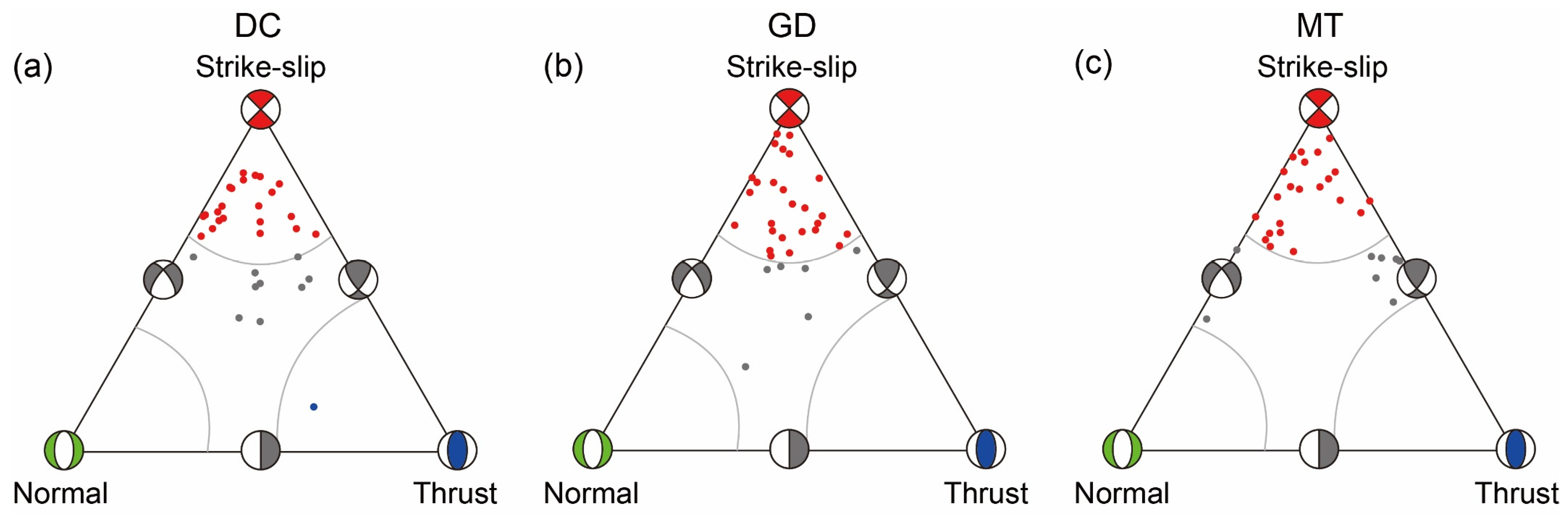
The inverted DC or GD fault plane results of different events are similar, the nodal lines of the GD results are very close (along the northeast or southwest direction), and the consistency between MT results is worse than the DC and GD results;

(2)

The non-DC mechanisms (represented by the relative proportion of shadow areas in the focal mechanism plots) and DC percentages of the GD and MT results show similar tendencies over time;

(3)

Most of the microseismic events occur at the middle and late HF stages. The main difference between the focal mechanisms of events in HF stages 1, 2, and 3 (Figure 7, Figure 8 and Figure 9) is the occurrence of a sequence of tensile and compressive mechanisms.

In HF stage 1 (Figure 7), the first two events have tensile mechanisms, and the other 9 events have compressive mechanisms, whereas in HF stages 2 and 3 (Figure 8 and Figure 9), the tensile and compressive sequence is not in order. In HF stage 2 (Figure 8), events B03, B07–B09, and B11 have tensile mechanisms, and the others have compressive mechanisms (the GD results of event B06 have only a 5% non-DC component; see Table S2 in the supplemental material). In HF stage 3 (Figure 9), events C02 and C06 have tensile mechanisms, and the others have compressive mechanisms.

We use rose diagrams (Figure 10) to illustrate the detailed distributions of the inverted strike, dip, and rake angles. From Figure 10, for all three models, more than half of the 32 events have dip angles greater than 75°, and their distributions of strike, dip, and rake angles are similar, except for the strike angles of nodal plane II.

Following Frohlich [43], we make triangle diagrams (Figure 11) to show the similarity and diversity of the determined focal mechanisms. As shown in Figure 11, the numbers of events with the strike-slip mechanism are 22, 26, and 24 for the DC, GD, and MT inversion results, respectively. This indicates that most of the 32 HF cracks have strike-slip mechanisms.

From the distribution of the results in the source type plot (Figure 12), most of the GD and MT results are located close to the boundaries, indicating significant non-DC components (tensile or compressive cracks). All the GD results are in the same straight line, which denotes the GD sources with $\nu$ of 0.25 in the source area.

5. Discussion

Different source models correspond to different constraints on the microseismic focal mechanism inversion. Because the DC, GD, and MT source models are described by four, five, and six parameters, respectively [28], their inversion performances may be different. In detail, the DC and GD inversions only need to search for three $\left(\phi ,\delta ,\lambda \right)$ and four $\left(\alpha ,\phi ,\delta ,\lambda \right)$ angles, respectively, which all have certain ranges, whereas during the MT inversion, the inverted six parameters $\left(M_{11},M_{22},M_{33},M_{12},M_{13},M_{23}\right)$ are very difficult to limit. In our previous work [28], the receiver array and velocity model shown in Figure 3 were used to compare the DC, GD, and MT inversions through numerical tests. According to the tests, for this single-well monitoring geometry, the GD and DC inversions are both stable, whereas the MT inversion deviates from the inputs in cases with 5% model velocity perturbations, 10 m horizontal source location errors, or 40% noise levels. We also find that the non-vertical direction of the monitoring well in Figure 3a–c is helpful for constraining single-well microseismic focal mechanism inversions [28].

We apply the DC, GD, and MT model-based focal mechanism inversions to a single-well field microseismic dataset to investigate the HF shear/tensile/compressive cracks. The inversion results with these three source models are compared in terms of the fault plane solution and DC percentages and linked to the HF stimulation curves. The results show the following:

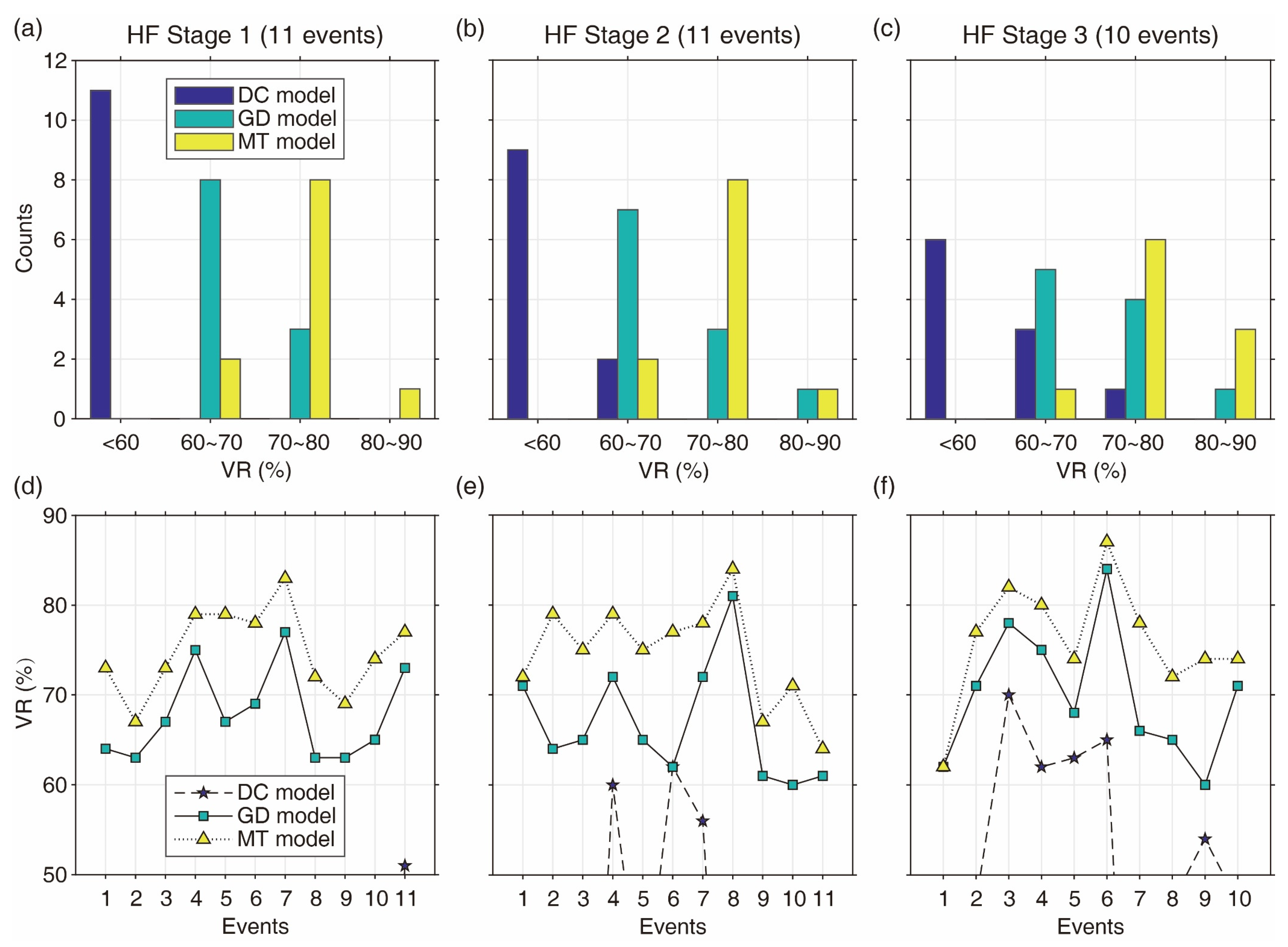
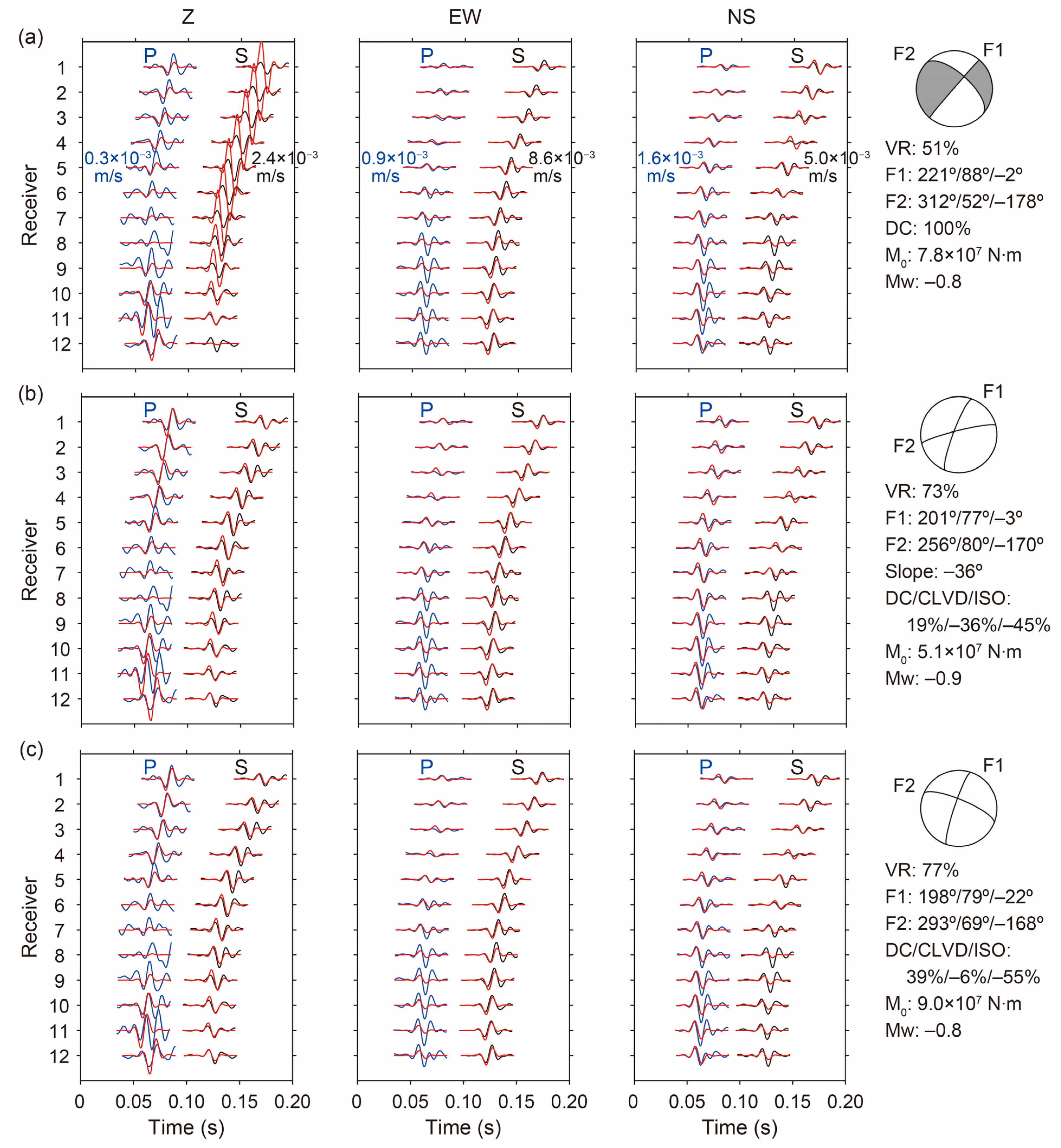
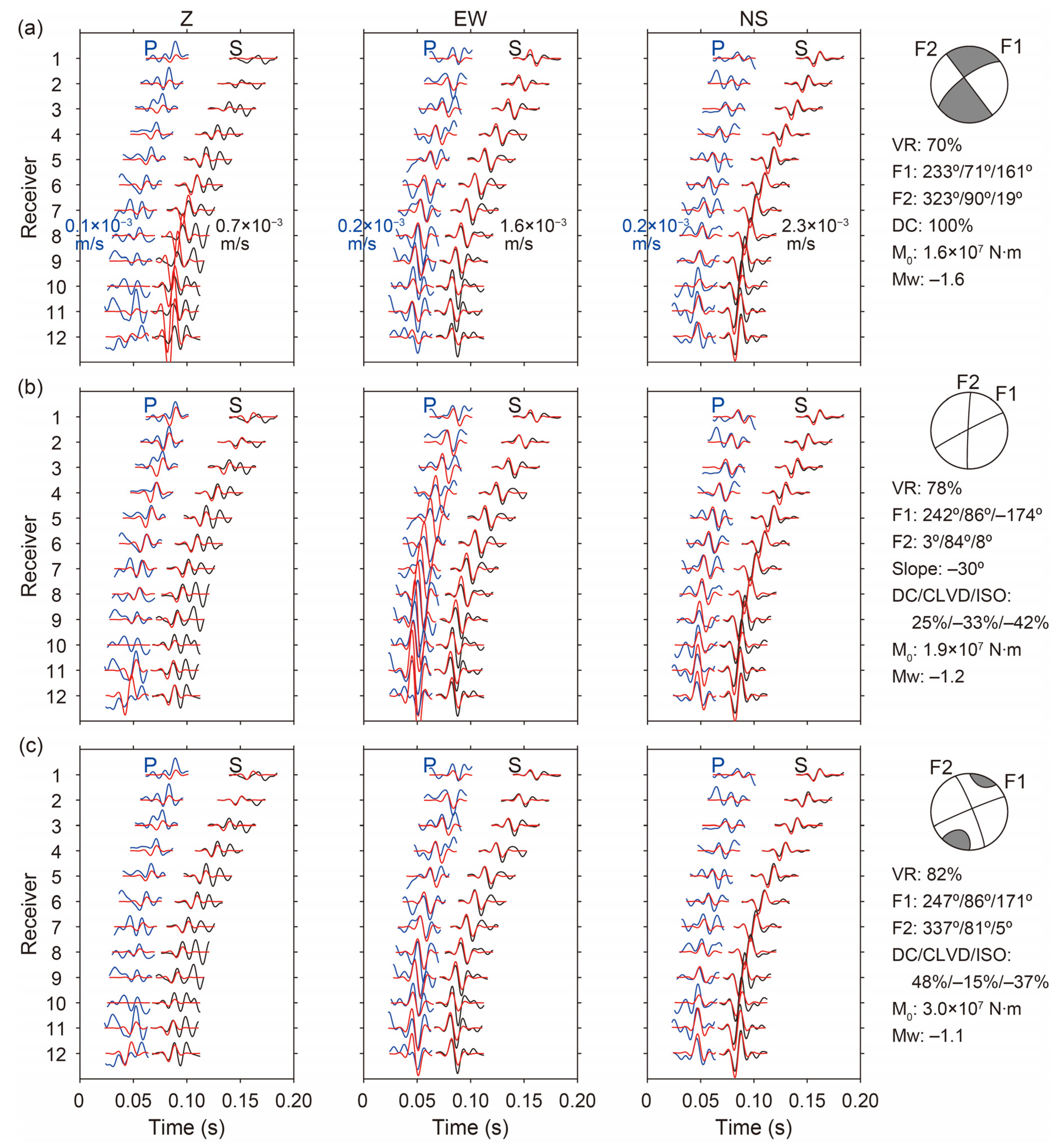
• The inversion quality (i.e., the goodness of fit between the observed data and synthetic seismograms, represented by the VR value) increases from DC → GD → MT (Figure 4), which is certain because the number of the model parameters increases from DC → GD → MT [46,47]. All the GD and MT results have VR values of ≥60%, whereas only 6 of 32 DC results have VR values in this range. Although the VR values of the MT results are better than those of the GD results, this does not mean that the MT results are certainly better. This is because: (1) the full MT inversion is not as stable as the GD inversions in our numerical tests with the same observation geometry [28] and in previous studies on acoustic emission events [26,48,49]; (2) for most of the 32 events, the difference between the VR values of the GD and MT results is not very large (see Figure 4d–f); and (3) from the GD to MT results in Figure 5 and Figure 6, the main improvement in the synthetic and observed waveform fitting (represented by the VR values) is related to the S/P amplitude ratio, which may be affected by the noise in the data.
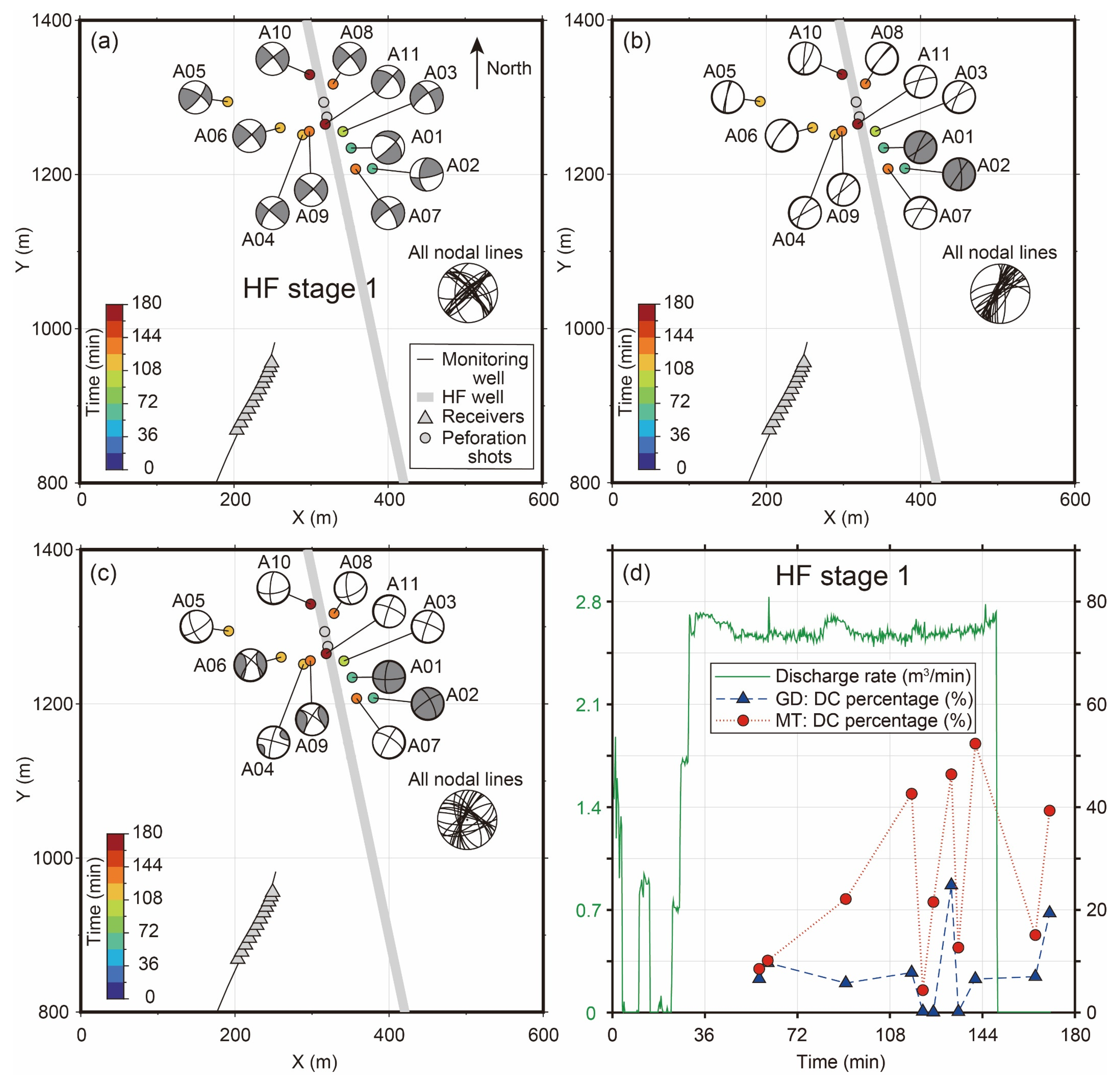
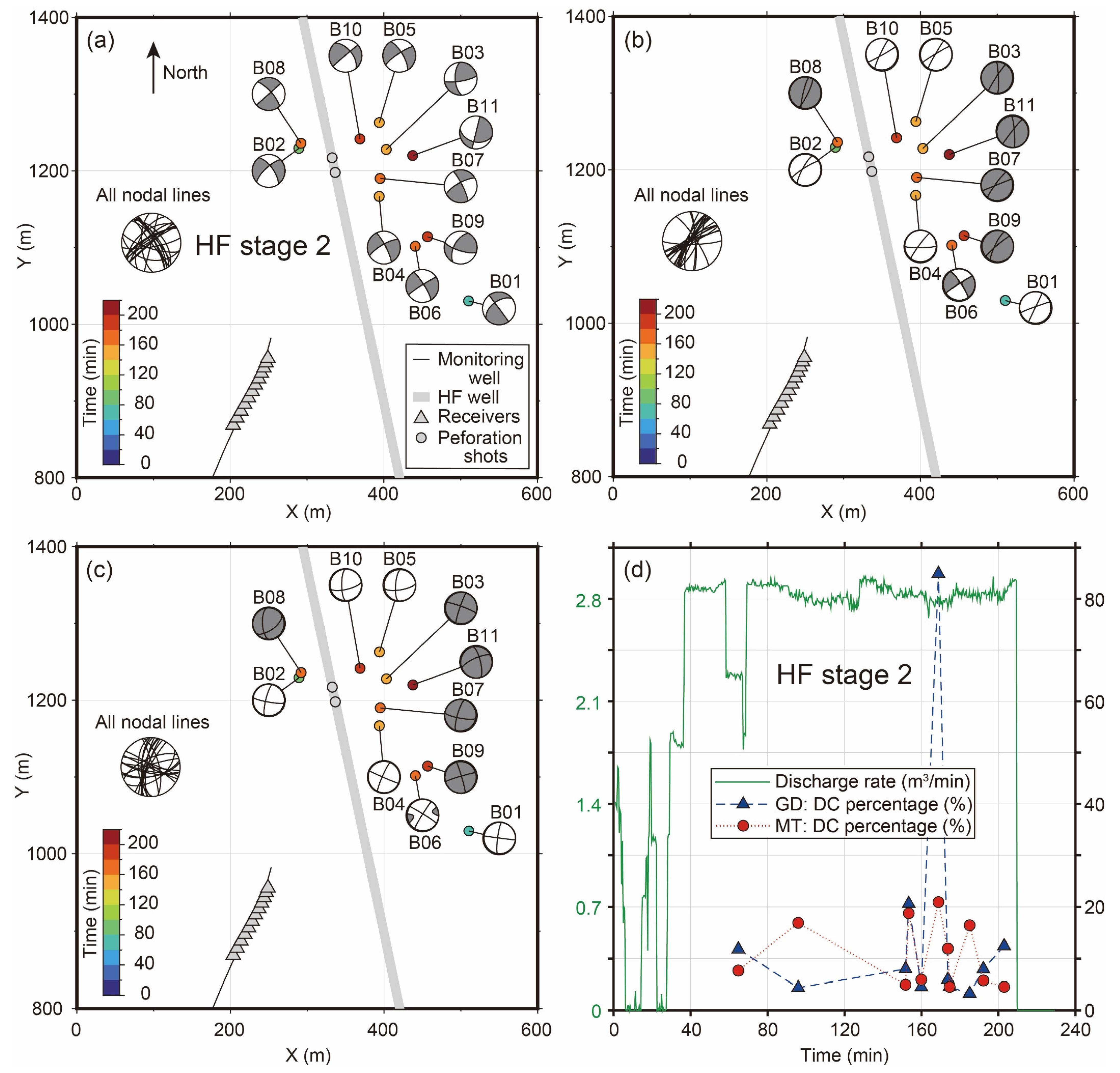
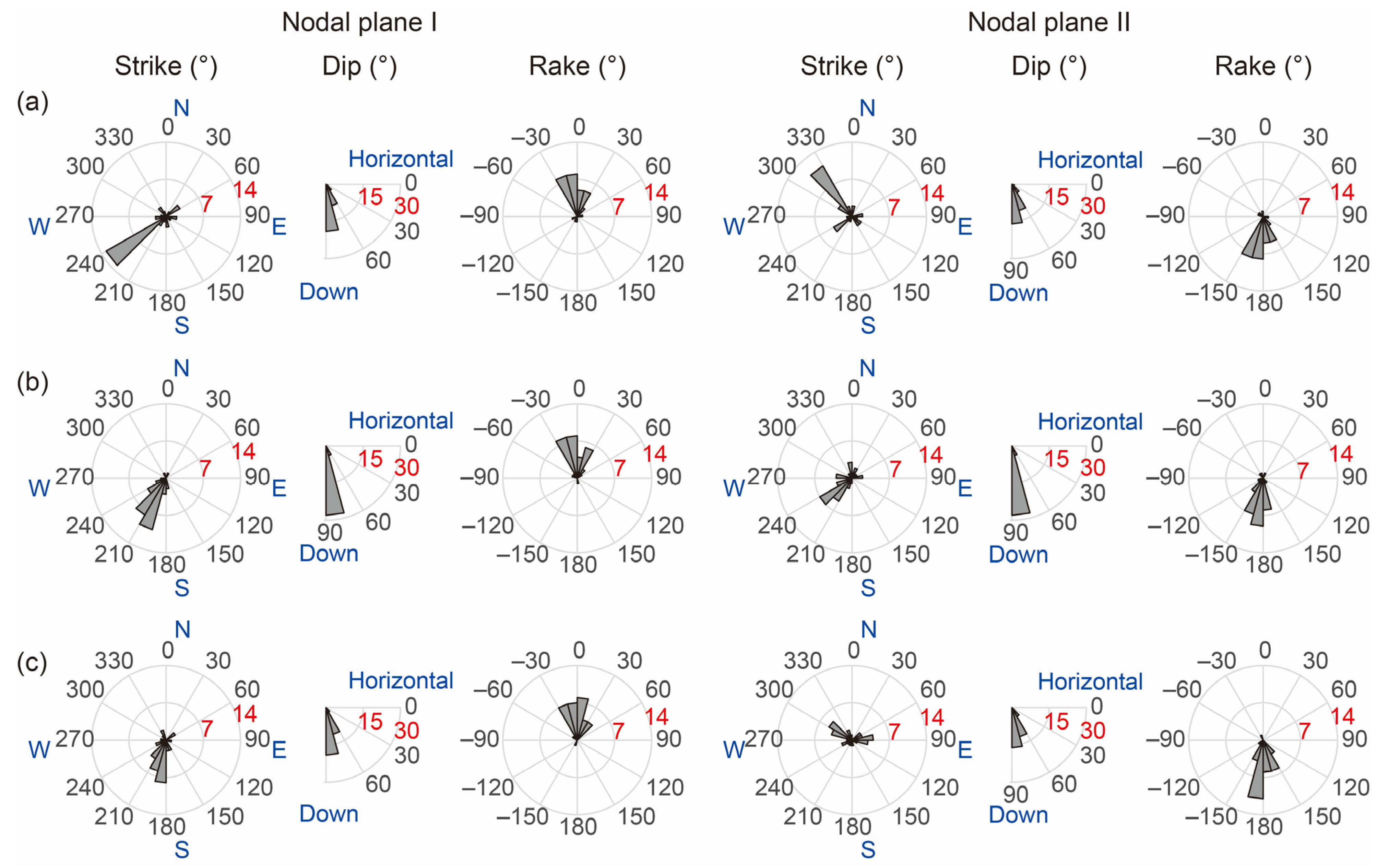
• In Figure 5, Figure 6, and Figure 10, the difference between the strike angle of nodal plane F2 (or II) from the GD results and that from the DC and MT results is quite large (>25°), whereas the other inverted parameters using these three models are similar. This may be because most of the inverted slope angles are non-zero (with –36° and –30° for events A11 and C03, respectively), and for a GD source with slope angle $\alpha \ne 0°$, the angle between its two possible nodal lines is not 90° (equal to $90°-\left|\alpha \right|$, where $\left|\alpha \right|$ is the absolute value of $\alpha$; refer to Li et al. [9]). Similar observations can also be found in the nodal lines shown in Figure 7, Figure 8 and Figure 9. Taking event A06 in Figure 7b as an example, we see that its two possible nodal lines are nearly the same. From Table S1, for event A06, the inverted slope angle is –87°, then the angle between its two possible nodal lines is $90°-\left|-87°\right|=3°$, and the inverted strike, dip, and rake angles of the two nodal lines are (214°, 73°, 22°) and (217°, 75°, 25°), respectively. Considering that the GD inversion is stable compared to the MT inversion in numerical tests using the same geometry [28] and the DC inversion quality for event A06 is very poor (with a VR of only –37%), we may draw the conclusion that event A06 is nearly a pure compressive crack occurring on a strike-slip fault with strike, dip, and rake angles of 214°–217°, 73°–75°, and 22°–25°, respectively. During the GD inversion, the non-zero slope angle can help to reduce the inversion uncertainty. The larger the inverted slope angle is, the smaller the angle between the two possible nodal lines (if the slope angle is nearly ±90°, the two possible nodal lines for a GD source are nearly the same [9]). According to the GD results in Figure 7, Figure 8, Figure 9, Figure 10 and Figure 11, the fracture geometry for most of the 32 events corresponds to shear/tensile/compressive strike-slip faulting, with strike angles of 195°–240° and dip angles of 75°–90°. These strike ranges are approximately perpendicular to the direction of the horizontal fracturing well. This is reasonable because during HF stimulations, the fracturing well is usually designed and set to be approximately perpendicular to the direction of the regional minimum principal stress. The inverted strike-slip fault type is also consistent with previous studies showing that strike-slip and dip-slip failures are two representative HF microseismic focal mechanisms [15,50,51].
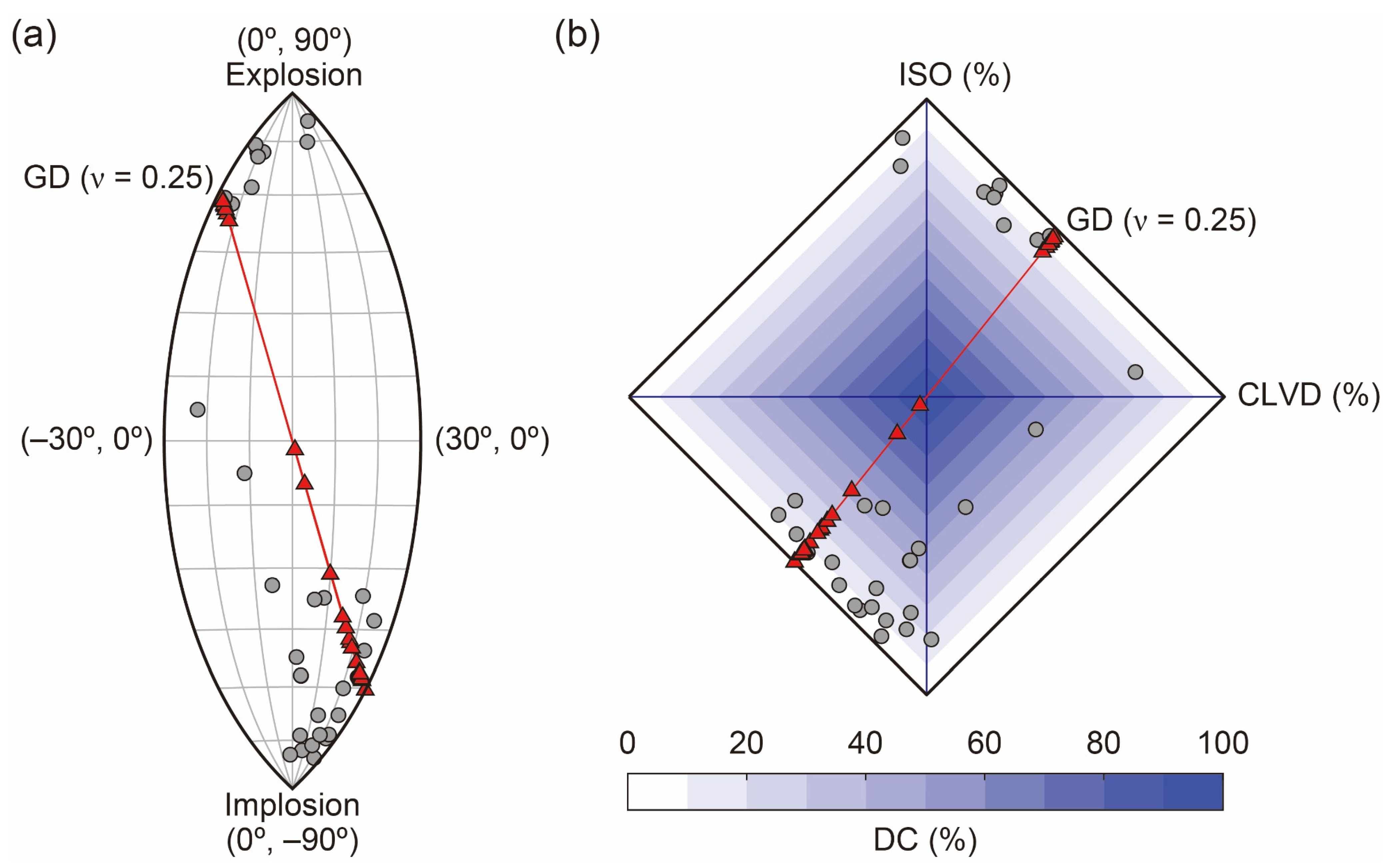
• From the DC percentage curves in Figure 7, Figure 8 and Figure 9, we see that the maximum difference between the GD and MT results is >60% (in Figure 8d). This is consistent with previous numerical tests using the same geometry, in which the MT inversion shows a maximum deviation of ~60% in terms of DC percentages [28]. According to the GD results, most of the HF cracks have non-negligible tensile/compressive mechanisms, especially in HF stage 1; all the microseismic events occur in the order of opening cracks first and then closing cracks. In this study, we use 32 events (with signal-to-noise ratio ≥ 4) to perform focal mechanism inversion. Future work involving this study will be related to data processing of the microseismic events with signal-to-noise ratio values of 2–4, in order to study the spatial-temporal distribution of shear/tensile/compressive HF cracks and the non-DC fracture growth in detail.

6. Conclusions

In this study, we apply the DC, GD, and MT model-based focal mechanism inversion methods to a single-well microseismic dataset to investigate the possible HF shear/tensile/compressive cracks. According to our study, the consistency between observed and synthetic microseismic waveforms (represented by the VR value) increases from DC → GD → MT. Most of the 32 microseismic events correspond to shear/tensile/compressive strike-slip faulting focal mechanisms. In most cases, the DC source model fails to fit the synthetic and observed waveforms well (with VR < 60%). The DC percentages between the GD and MT inversion results are significant (up to 60%) and consistent with the numerical test results in our previous work [28], in that the DC percentage of the MT inversion may deviate from the correct value by ~60%. For single-well microseismic focal mechanism inversion, the GD model is more suitable than the DC and MT models because it considers the non-DC mechanism and yields a stable inversion process. Moreover, the inverted non-zero slope angle using the GD model can help to reduce the uncertainty in fracture geometry characterization. In some cases, the inverted slope angle is approximately ±90°, and the two possible fault planes are nearly the same. Our study provides a useful example of how to investigate HF fracture geometry and shear/tensile/compressive mechanisms with downhole microseismic data, which will help improve microseismic studies and HF evaluations for enhanced resource recovery.

References

1. Maxwell, S.C.; Urbancic, T.I. The Role of Passive Microseismic Monitoring in the Instrumented Oil Field. Lead. Edge 2001, 20, 636–639. [Google Scholar] [CrossRef]
2. Li, L.; Tan, J.; Wood, D.A.; Zhao, Z.; Becker, D.; Lyu, Q.; Shu, B.; Chen, H. A Review of the Current Status of Induced Seismicity Monitoring for Hydraulic Fracturing in Unconventional Tight Oil and Gas Reservoirs. Fuel 2019, 242, 195–210. [Google Scholar] [CrossRef]
3. Li, H.; Chang, X. A Review of the Microseismic Focal Mechanism Research. Sci. China Earth Sci. 2021, 64, 351–363. [Google Scholar] [CrossRef]
4. Wamriew, D.; Dorhjie, D.B.; Bogoedov, D.; Pevzner, R.; Maltsev, E.; Charara, M.; Pissarenko, D.; Koroteev, D. Microseismic Monitoring and Analysis Using Cutting-Edge Technology: A Key Enabler for Reservoir Characterization. Remote Sens. 2022, 14, 3417. [Google Scholar] [CrossRef]
5. Ma, C.; Yan, W.; Xu, W.; Li, T.; Ran, X.; Wan, J.; Tong, K.; Lin, Y. Parallel Processing Method for Microseismic Signal Based on Deep Neural Network. Remote Sens. 2023, 15, 1215. [Google Scholar] [CrossRef]
6. Baig, A.; Urbancic, T. Microseismic Moment Tensors: A Path to Understanding Frac Growth. Lead. Edge 2010, 29, 320–324. [Google Scholar] [CrossRef]
7. Maxwell, S.C.; Chorney, D.; Goodfellow, S.D. Microseismic Geomechanics of Hydraulic-Fracture Networks: Insights into Mechanisms of Microseismic Sources. Lead. Edge 2015, 34, 904–910. [Google Scholar] [CrossRef]
8. Vavryčuk, V. Tensile Earthquakes: Theory, Modeling, and Inversion. J. Geophys. Res. Solid Earth 2011, 116, B12320. [Google Scholar] [CrossRef]
9. Li, H.; Chang, X.; Hao, J.; Wang, Y. The General Dislocation Source Model and Its Application to Microseismic Focal Mechanism Inversion. Geophysics 2021, 86, KS79–KS93. [Google Scholar] [CrossRef]
10. Minson, S.E.; Dreger, D.S. Stable Inversions for Complete Moment Tensors. Geophys. J. Int. 2008, 174, 585–592. [Google Scholar] [CrossRef]
11. Alvizuri, C.; Silwal, V.; Krischer, L.; Tape, C. Estimation of Full Moment Tensors, Including Uncertainties, for Nuclear Explosions, Volcanic Events, and Earthquakes. J. Geophys. Res. Solid Earth 2018, 123, 5099–5119. [Google Scholar] [CrossRef]
12. Eaton, D.W.; Forouhideh, F. Solid Angles and the Impact of Receiver-Array Geometry on Microseismic Moment-Tensor Inversion. Geophysics 2011, 76, WC77–WC85. [Google Scholar] [CrossRef]
13. Shang, X.; Tkalčić, H. Point-Source Inversion of Small and Moderate Earthquakes From P-wave Polarities and P/S Amplitude Ratios Within a Hierarchical Bayesian Framework: Implications for the Geysers Earthquakes. J. Geophys. Res. Solid Earth 2020, 125, e2019JB018492. [Google Scholar] [CrossRef]
14. Šílený, J. Resolution of Non-Double-Couple Mechanisms: Simulation of Hypocenter Mislocation and Velocity Structure Mismodeling. Bull. Seismol. Soc. Am. 2009, 99, 2265–2272. [Google Scholar] [CrossRef]
15. Staněk, F.; Eisner, L.; Jan Moser, T. Stability of Source Mechanisms Inverted from P-Wave Amplitude Microseismic Monitoring Data Acquired at the Surface. Geophys. Prospect. 2014, 62, 475–490. [Google Scholar] [CrossRef]
16. Julian, B.R.; Miller, A.D.; Foulger, G.R. Non-Double-Couple Earthquakes (1) Theory. Rev. Geophys. 1998, 36, 525–549. [Google Scholar] [CrossRef]
17. Eyre, T.S.; van der Baan, M. The Reliability of Microseismic Moment-Tensor Solutions: Surface versus Borehole Monitoring. Geophysics 2017, 82, KS113–KS125. [Google Scholar] [CrossRef]
18. Vavryčuk, V. Inversion for Parameters of Tensile Earthquakes. J. Geophys. Res. Solid Earth 2001, 106, 16339–16355. [Google Scholar] [CrossRef]
19. Šílený, J.; Jechumtálová, Z.; Dorbath, C. Small Scale Earthquake Mechanisms Induced by Fluid Injection at the Enhanced Geothermal System Reservoir Soultz (Alsace) in 2003 Using Alternative Source Models. Pure Appl. Geophys. 2014, 171, 2783–2804. [Google Scholar] [CrossRef]
20. Kwiatek, G.; Ben-Zion, Y. Assessment of P and S Wave Energy Radiated from Very Small Shear-Tensile Seismic Events in a Deep South African Mine. J. Geophys. Res. Solid Earth 2013, 118, 3630–3641. [Google Scholar] [CrossRef]
21. Dahm, T.; Manthei, G.; Eisenblätter, J. Automated Moment Tensor Inversion to Estimate Source Mechanisms of Hydraulically Induced Micro-Seismicity in Salt Rock. Tectonophysics 1999, 306, 1–17. [Google Scholar] [CrossRef]
22. Šílený, J.; Horálek, J. Shear-Tensile Crack as a Tool for Reliable Estimates of the Non-Double-Couple Mechanism: West Bohemia-Vogtland Earthquake 1997 Swarm. Phys. Chem. Earth 2016, 95, 113–124. [Google Scholar] [CrossRef]
23. Dufumier, H.; Rivera, L. On the Resolution of the Isotropic Component in Moment Tensor Inversion. Geophys. J. Int. 1997, 131, 595–606. [Google Scholar] [CrossRef]
24. Tape, W.; Tape, C. The Classical Model for Moment Tensors. Geophys. J. Int. 2013, 195, 1701–1720. [Google Scholar] [CrossRef]
25. Stierle, E.; Vavryčuk, V.; Šílený, J.; Bohnhoff, M. Resolution of Non-Double-Couple Components in the Seismic Moment Tensor Using Regional Networks-i: A Synthetic Case Study. Geophys. J. Int. 2014, 196, 1869–1877. [Google Scholar] [CrossRef]
26. Petružálek, M.; Jechumtálová, Z.; Kolář, P.; Adamová, P.; Svitek, T.; Šílený, J.; Lokajíček, T. Acoustic Emission in a Laboratory: Mechanism of Microearthquakes Using Alternative Source Models. J. Geophys. Res. Solid Earth 2018, 123, 4965–4982. [Google Scholar] [CrossRef]
27. Pesicek, J.D.; Sileny, J.; Prejean, S.G.; Thurber, C.H. Determination and Uncertainty of Moment Tensors for Microearthquakes at Okmok Volcano, Alaska. Geophys. J. Int. 2012, 190, 1689–1709. [Google Scholar] [CrossRef]
28. Li, H.; Chang, X.; Hao, J.; Wang, Y. Comparison of Single-Well Microseismic Focal Mechanism Inversions with Different Source Models. Bull. Seismol. Soc. Am. 2021, 111, 3103–3117. [Google Scholar] [CrossRef]
29. Aki, K.; Richards, P.G. Quantitative Seismology, 2nd ed.; University Science Books: Mill Valley, CA, USA, 2002; ISBN 0-935702-96-2. [Google Scholar]
30. Ou, G. Bin Seismological Studies for Tensile Faults. Terr. Atmos. Ocean. Sci. 2008, 19, 463–471. [Google Scholar] [CrossRef]
31. Langston, C.A. Source Inversion of Seismic Waveforms: The Koyna, India, Earthquakes of 13 September 1967. Bull. Seismol. Soc. Am. 1981, 71, 1–24. [Google Scholar] [CrossRef]
32. Yao, Z.; Harkrider, D.G. A Generalized Reflection-Transmission Coefficient Matrix and Discrete Wavenumber Method for Synthetic Seismograms. Bull. Seismol. Soc. Am. 1983, 73, 1685–1699. [Google Scholar]
33. Rothman, D.H. Automatic Estimation of Large Residual Statics Corrections. Geophysics 1986, 51, 332–346. [Google Scholar] [CrossRef]
34. Yao, Z.; Ji, C. The Inverse Problem of Finite Fault Study in Time Domain. Chin. J. Geophys. 1997, 5, 691–701. [Google Scholar]
35. Song, F.; Toksöz, M.N. Full-Waveform Based Complete Moment Tensor Inversion and Source Parameter Estimation from Downhole Microseismic Data for Hydrofracture Monitoring. Geophysics 2011, 76, WC103–WC116. [Google Scholar] [CrossRef]
36. Jost, M.L.; Herrmann, R.B. A Student’s Guide to and Review of Moment Tensors. Seismol. Res. Lett. 1989, 60, 37–57. [Google Scholar] [CrossRef]
37. Kanamori, H. The Energy Release in Great Earthquakes. J. Geophys. Res. 1977, 82, 2981–2987. [Google Scholar] [CrossRef]
38. Knopoff, L.; Randall, M.J. The Compensated Linear-Vector Dipole: A Possible Mechanism for Deep Earthquakes. J. Geophys. Res. 1970, 75, 4957–4963. [Google Scholar] [CrossRef]
39. Chiang, A.; Ichinose, G.A.; Dreger, D.S.; Ford, S.R.; Matzel, E.M.; Myers, S.C.; Walter, W.R. Moment Tensor Source-Type Analysis for the Democratic People’s Republic of Korea-Declared Nuclear Explosions (2006–2017) and 3 September 2017 Collapse Event. Seismol. Res. Lett. 2018, 89, 2152–2165. [Google Scholar] [CrossRef]
40. Krížová, D.; Málek, J. Focal Mechanisms of West Bohemia, Central Europe, Earthquakes-End of May 2014: Evidence of Volume Changes. Seismol. Res. Lett. 2021, 92, 3398–3415. [Google Scholar] [CrossRef]
41. Li, X.S.; Wu, L.P.; Yin, L.; Judd, T. An Integrated Disciplinary Approach towards Hydraulic Fracturing Optimization of Tight Oil Wells in the Ordos Basin, China. In Proceedings of the SPE Asia Pacific Unconventional Resources Conference and Exhibition, Brisbane, QLD, Australia, 11 November 2013; Volume 2, pp. 631–642. [Google Scholar]
42. Hubbert, M.K.; Willis, D.G. Mechanics Of Hydraulic Fracturing. Trans. AIME 1957, 210, 153–168. [Google Scholar] [CrossRef]
43. Frohlich, C. Triangle Diagrams: Ternary Graphs to Display Similarity and Diversity of Earthquake Focal Mechanisms. Phys. Earth Planet. Inter. 1992, 75, 193–198. [Google Scholar] [CrossRef]
44. Tape, W.; Tape, C. A Geometric Setting for Moment Tensors. Geophys. J. Int. 2012, 190, 476–498. [Google Scholar] [CrossRef]
45. Vavryčuk, V. Moment Tensor Decompositions Revisited. J. Seismol. 2015, 19, 231–252. [Google Scholar] [CrossRef]
46. Menke, W. Geophysical Data Analysis: Discrete Inverse Theory; Academic press: Cambridge, MA, USA, 2018. [Google Scholar]
47. Aster, R.C.; Borchers, B.; Thurber, C.H. Parameter Estimation and Inverse Problems, 3rd ed.; Elsevier: Amsterdam, The Netherlands, 2019. [Google Scholar]
48. Petružálek, M.; Jechumtálová, Z.; Šílený, J.; Kolář, P.; Svitek, T.; Lokajíček, T.; Turková, I.; Kotrlý, M.; Onysko, R. Application of the Shear-Tensile Source Model to Acoustic Emissions in Westerly Granite. Int. J. Rock Mech. Min. Sci. 2020, 128, 104246. [Google Scholar] [CrossRef]
49. Ren, Y.; Vavryčuk, V.; Wu, S.; Gao, Y. Accurate Moment Tensor Inversion of Acoustic Emissions and Its Application to Brazilian Splitting Test. Int. J. Rock Mech. Min. Sci. 2021, 141, 104707. [Google Scholar] [CrossRef]
50. Rutledge, J.T.; Phillips, W.S. Hydraulic Stimulation of Natural Fractures as Revealed by Induced Microearthquakes, Carthage Cotton Valley Gas Field, East Texas. Geophysics 2003, 68, 441–452. [Google Scholar] [CrossRef]
51. Eisner, L.; Williams-Stroud, S.; Hill, A.; Duncan, P.; Thornton, M. Beyond the Dots in the Box: Microseismicity-Constrained Fracture Models for Reservoir Simulation. Lead. Edge 2010, 29, 326–333. [Google Scholar] [CrossRef]
52. Tape, W.; Tape, C. Angle between Principal Axis Triples. Geophys. J. Int. 2012, 191, 813–831. [Google Scholar] [CrossRef]
53. Tape, W.; Tape, C. A Uniform Parametrization of Moment Tensors. Geophys. J. Int. 2015, 202, 2074–2081. [Google Scholar] [CrossRef]
Figure 1. Illustrations of the (a) double-couple (DC) and (b) general dislocation (GD) models. n and [u] are the fault normal and slip vectors, respectively. uDC is the shear slip component of the slip vector [u]. α is the slope angle [8], i.e., the angle between [u] and uDC.
Remotesensing 16 01902 g001
Figure 2. Map showing the locations of the HF site and the monitoring well in the Ordos Basin, China. The squares denote the locations of nearby cities.
Remotesensing 16 01902 g002
Figure 3. Geometry of the injection and monitoring wells, locations of the microseismic events, and velocity models. There are three HF stages, each with two fluid injection points (shown as crosses). The monitoring system consists of 12 three-component receivers (shown as grey triangles). Selected events in HF stages 1, 2, and 3 are shown as squares, inverted triangles, and circles, respectively. The total event number is 32, with 11, 11, and 10 events in HF stages 1, 2, and 3, respectively. (ac) Map and side views. (d) P- and S-wave well log data (dotted lines) and velocities (solid lines).
Remotesensing 16 01902 g003
Figure 4. Histograms (ac) and distributions (df) of the VR values for the microseismic focal mechanism inversions in three HF stages with the DC, GD, and MT models. Note that only VR values greater than 50% are shown.
Remotesensing 16 01902 g004
Figure 5. Waveform fitting and focal mechanism inversion results for event A11 (location shown in Figure 3a–c). Rows (ac) indicate the results using the DC, GD, and MT models, respectively. The black and blue lines indicate the observed P and S waveforms (filtered and normalized with respect to those at receiver 5, whose amplitudes are listed in the panels), respectively. The red lines indicate the synthetic data. F1 and F2 (with parameters listed in the order of strike/dip/rake angles) are two fault planes corresponding to the same seismograms.
Remotesensing 16 01902 g005
Figure 6. Waveform fitting and focal mechanism inversion results for event C03 (location shown in Figure 3a–c). Rows (ac) indicate the results using the DC, GD, and MT models, respectively. The black and blue lines indicate the observed P and S waveforms (normalized with respect to those at receiver 8, whose amplitudes are listed in the panels), respectively. The red lines indicate the synthetic data. F1 and F2 (with parameters listed in the order of strike/dip/rake angles) are two fault planes corresponding to the same seismograms.
Remotesensing 16 01902 g006
Figure 7. Inverted focal mechanism plots of the 11 events in HF stage 1 (marked as A01–A11) using the (a) DC, (b) GD, and (c) MT models. (d) Variations in the fluid discharge rate and the inverted DC percentages using the GD and MT models.
Remotesensing 16 01902 g007
Figure 8. Inverted focal mechanism plots of the 11 events in HF stage 2 (marked as B01–B11) using the (a) DC, (b) GD, and (c) MT models. (d) Variations in the fluid discharge rate and the inverted DC percentages using the GD and MT models.
Remotesensing 16 01902 g008
Figure 9. Inverted focal mechanism plots of the 10 events in HF stage 3 (marked as C01–C10) using the (a) DC, (b) GD, and (c) MT models. (d) Variations in the fluid discharge rate and the inverted DC percentages using the GD and MT models.
Remotesensing 16 01902 g009
Figure 10. Rose diagrams of the strike, dip, and rake angles of the two inverted nodal planes for the 32 microseismic events. (ac) Results using the DC, GD, and MT models (blue for the directions and red for the counts of angle values in certain ranges).
Remotesensing 16 01902 g010
Figure 11. Triangle diagrams [43] of the focal mechanisms inverted using the (a) DC, (b) GD, and (c) MT source models. The red, green, and blue points indicate the strike-slip, normal, and thrust mechanisms, respectively. The gray ones indicate the odd mechanism defined by Frohlich [43].
Remotesensing 16 01902 g011
Figure 12. Distribution of all the GD and MT inversion results in two different source-type plots. The red triangles indicate the GD results (with fixed ν of 0.25) and the gray dots denote the MT results. (a) The 2-D equal-area projection plot of the fundamental lune [24]. The upper left and lower right boundaries indicate pure tensile and pure compressive mechanisms, respectively. The pure shear (DC) mechanism is located in the center. The coordinates of the boundaries are in the order of γ ,   δ , where γ and δ are the longitude ( γ [ 30 ° ,   30 ° ] ) and latitude ( δ [ 90 ° ,   90 ° ] ) on the eigenvalue lune that determine the source pattern [44]. (b) The diamond CLVD-ISO percentage plot [45]. The upper right and lower left boundaries indicate pure tensile and pure compressive mechanisms, respectively. The pure shear (DC) mechanism locates in the center.
Remotesensing 16 01902 g012
Disclaimer/Publisher’s Note: The statements, opinions and data contained in all publications are solely those of the individual author(s) and contributor(s) and not of MDPI and/or the editor(s). MDPI and/or the editor(s) disclaim responsibility for any injury to people or property resulting from any ideas, methods, instructions or products referred to in the content.