Improving the Accuracy of Digital Terrain Models Using Drone-Based LiDAR for the Morpho-Structural Analysis of Active Calderas: The Case of Ischia Island, Italy

Abstract

Over the past two decades, the airborne Light Detection and Ranging (LiDAR) system has become a useful tool for acquiring high-resolution topographic data, especially in active tectonics studies. Analyzing Digital Terrain Models (DTMs) from LiDAR exposes morpho-structural elements, aiding in the understanding of fault zones, among other applications. Despite its effectiveness, challenges persist in regions with rapid deformation, dense vegetation, and human impact. We propose an adapted workflow transitioning from the conventional airborne LiDAR system to the usage of drone-based LiDAR technology for higher-resolution data acquisition. Additionally, drones offer a more cost-effective solution, both in an initial investment and ongoing operational expenses. Our goal is to demonstrate how drone-based LiDAR enhances the identification of active deformation features, particularly for earthquake-induced surface faulting. To evaluate the potential of our technique, we conducted a drone-based LiDAR survey in the Casamicciola Terme area, north of Ischia Island, Italy, known for the occurrence of destructive shallow earthquakes, including the 2017 Md = 4 event. We assessed the quality of our acquired DTM by comparing it with existing elevation datasets for the same area. We discuss the advantages and limitations of each DTM product in relation to our results, particularly when applied to fault mapping. By analyzing derivative DTM products, we identified the fault scarps within the Casamicciola Holocene Graben (CHG) and mapped its structural geometry in detail. The analysis of both linear and areal geomorphic features allowed us to identify the primary factors influencing the current morphological arrangement of the CHG area. Our detailed map depicts a nested graben formed by two main structures (the Maio and Sentinella faults) and minor internal faults (the Purgatorio and Nizzola faults). High-resolution DEMs acquired by drone-based LiDAR facilitated detailed studies of the geomorphology and fault activity. A similar approach can be applied in regions where the evidence of high slip-rate faults is difficult to identify due to vegetation cover and inaccessibility.

1. Introduction

LiDAR (Light Detection and Ranging) technology has been a tool for collecting thousands of georeferenced geographic positioning points per second to produce high-resolution Digital Elevation Models (DEMs). A significant advantage of the LiDAR systems is the capacity of the laser beam to penetrate densely vegetated areas and accurately measure distances to the ground beneath [1], whereas, for example, with photogrammetry techniques, the vegetation is deleted by estimating the height, potentially impacting the accuracy of the resulting topography [2].

LiDAR systems operated from airplanes and helicopters have been widely applied to earth science and other investigations [3,4,5,6,7,8,9,10], facilitating the coverage of relatively large areas in a short amount of time, showing a high resistance to interference, and remaining unaffected by illumination conditions, such as shadows [2,11,12]. Therefore, LiDAR stands out as a unique remote-sensing technique capable of accurately detecting geomorphological features in entirely or partly vegetated areas. However, its application through manned aircraft is non-cost effective.

On the contrary, the recent popularity of drone systems and the advances in lightweight LiDAR sensors allow for a less expensive and easier way to join both systems as a source of data elevation acquisition. Drone-based LiDAR provides easier access to hazardous sites with minimal human intervention. The ability to fly at various elevations and speeds enables data acquisition at different resolutions. These qualities are particularly useful in volcano–tectonic areas, which often show a complex topography at a local scale.

Although the usage of drone-based LiDAR is widely known in archaeology, ecology, and construction [13], there are very few records of its application in geomorphology, active tectonics, and morpho-structural studies [14,15,16]. The main objective of this paper is to propose a reproducible methodology for deriving DEMs from drone-based LiDAR. The aim is to assess the applicability of this tool to enhance geomorpho-structural analysis by extracting landform features from very high-resolution topographic data. This is helpful in analyzing the ground deformation and ground ruptures [17,18] caused by volcanotectonic structures characterized by rapid fault slip rates and high rates of Holocene deformation (e.g., Mt. Etna, Italy [19]; Campi Flegrei, Italy [20]; Los Humeros Caldera, Mexico [21,22]; Galeras Volcano, Colombia [23]).

We tested the method in the volcanic Ischia Island (Figure 1), where a moderate, (Md = 4.0 and I = VII ESI scale [24,25] and references therein) shallow earthquake (1.5 km depth) hit the Casamicciola Terme on the 21 August 2017, causing severe damage and two casualties (Figure 2).

The epicentral location of the 2017 earthquake [34] and the destructive pre-instrumental earthquakes (1796, 1828, 1881, and 1883, [35] and references therein) were confined to the same area of few square kilometers. The clear stratigraphic and morphological evidence of the seismo-tectonic activity is represented by the Casamicciola Holocene Graben (CHG) located at the base of the northern flank of Mt. Epomeo (Figure 2) [25]. The 2017 seismic event produced primary coseismic surface ruptures related to the earthquake-causative fault and secondary coseismic effects [24] mostly related to ground shaking, such as landslides and hydrological variations [36,37,38,39], mapped and reported in detail by Nappi et al. (2018) and Nappi et al. (2020) [24,40].

The primary coseismic fault ruptures reactivated a ca. 2 km segment along the E-trending and N-dipping normal fault, which runs at the base of Mt. Epomeo and forms the master fault of the CHG [24,25,41,42,43]. However, more faulting evidence is needed, between the mapped coseismic ruptures by Nappi et al. (2018) [24] and the progressive offset along the normal fault of the northern flank of Mt. Epomeo. We considered that a first-time drone-based LiDAR survey could fill this evidence gap, which was previously hidden by vegetation and inaccessible areas.

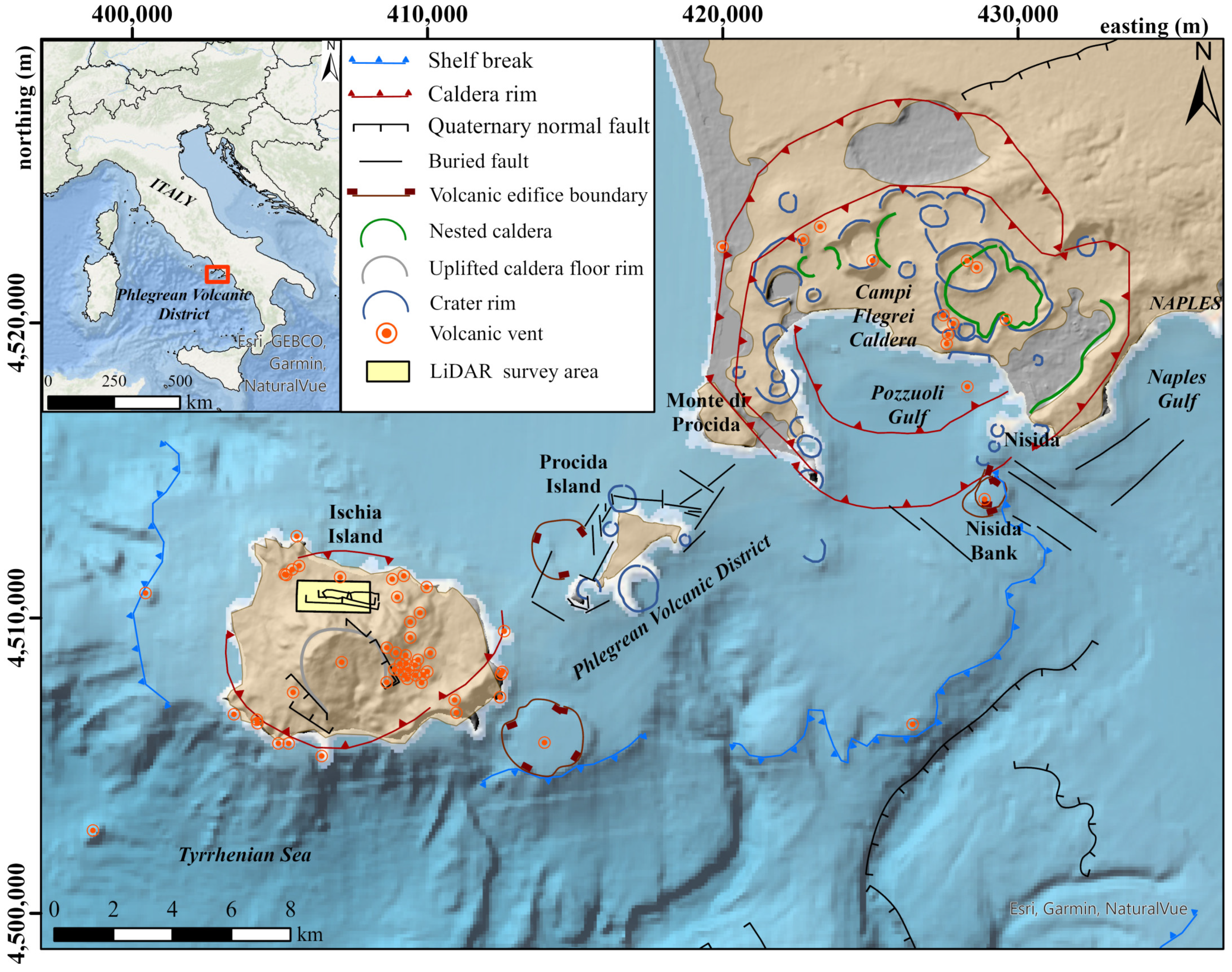
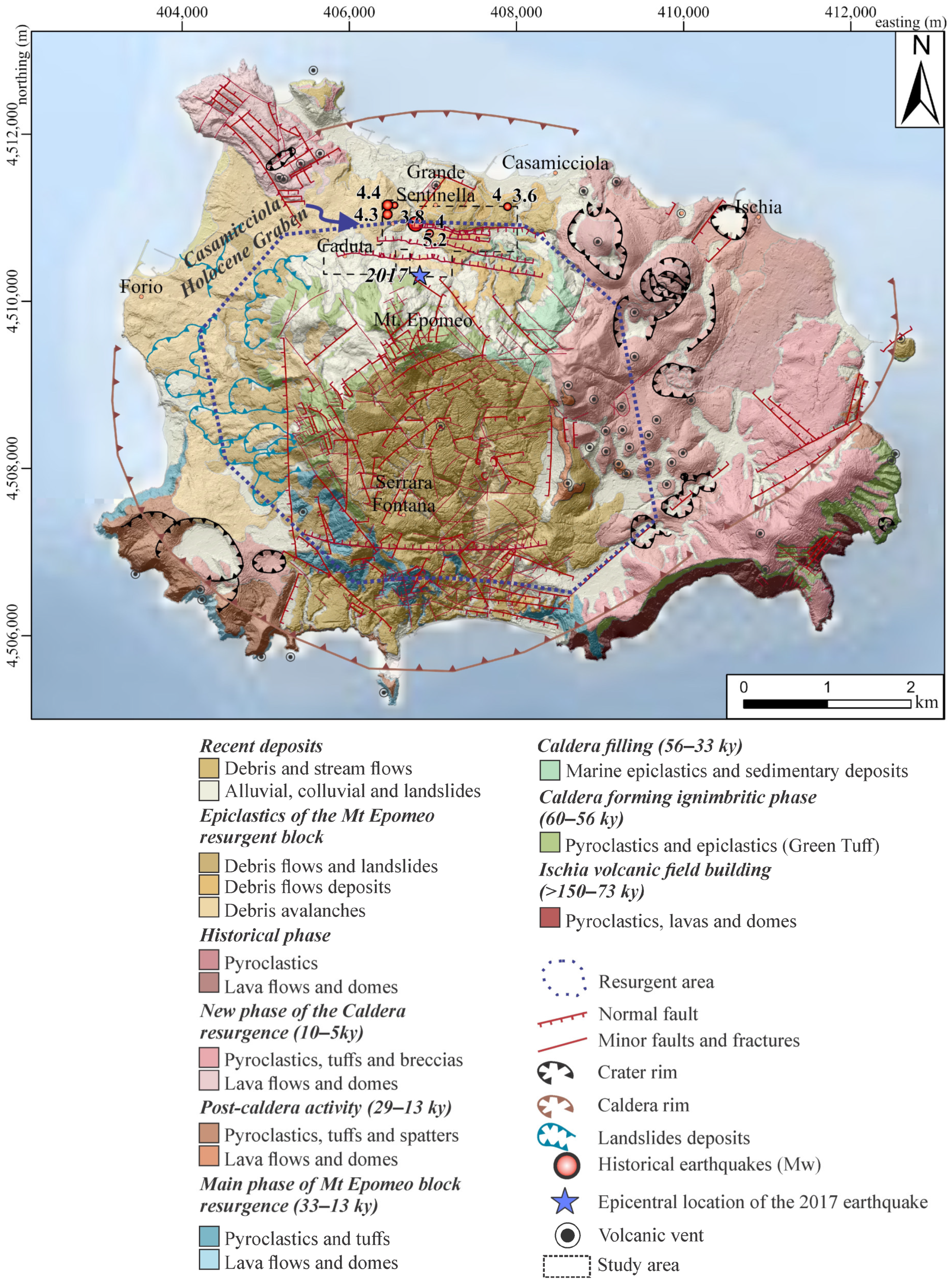
2. Geological and Seismological Background

Ischia Island is a resurgent caldera active prior to 150 ky B.P. and during historical times [32,44,45]. Ischia belongs to the Campanian volcanic district in the west of the Gulf of Naples, Italy (Figure 1) [29,30,31,46]. The island extends 46 km² and is covered by volcanic products resulting from different explosive and effusive eruptions. The main morpho-structural features are (1) the caldera rim along the border of the island and (2) the relief of Mt. Epomeo as a structural high of 787 m a.s.l, covering approximately 9 km² [25].

The caldera formation event occurred about 60–56 ky B.P., triggered and controlled by the Mt. Epomeo Green Tuff eruption (9–15 km³ estimated volume of erupted magma, [47]). The caldera depression was partially filled by epiclastic sedimentation in marine environments during a period of stasis in volcanism dated about 56 to 33 ky B.P. (Figure 2) [31,48].

The variations in the pressure and volume of the magmatic and hydrothermal systems led to the resurgence of the caldera floor, as it is particularly common in the caldera-forming process [49,50,51]. This stage started at 33 ky B.P. with following episodic uplifts of Mt. Epomeo [48] due to variations in magmatic intrusions [30,44], causing the asymmetric morphology of the island [30]. The E–ENE normal fault system that borders the N flank of Mt. Epomeo has accommodated a maximum vertical displacement of ca. 1 km [30,31,32,33,45,48,52,53]. In the foothill area of Casamicciola Terme, a structure, part of the E-ENE fault system, separates Mt. Epomeo from the coastal area and forms the Casamicciola Holocene Graben (CHG) (Figure 2) [25,54].

Destructive and shallow volcano–tectonic earthquakes occurred recurrently in the hilly part of the Casamicciola Terme area during the last three centuries in 1796, 1828, 1881, 1883, and 2017 [55,56,57,58,59]. These earthquakes resulted in significant damage to the Casamicciola area and its surroundings. The 1883 earthquake was one of the worst seismic events in the Italian seismic catalog, with more than 2300 casualties [58]. The latest event, in August 2017, was the first damaging earthquake of the instrumental era, recorded by seismological, geodetic, geophysical, and field mapping data. It was characterized by a shallow hypocentral depth of around 1.2 km, with an E-trending normal fault plane as the seismogenic source [24,34,60]. The main factors contributing to the extensive destruction were as follows: (1) the shallow nature of the seismogenic source, (2) complications resulting from site-specific amplification due to geological variations in the epicentral area, and (3) the poor construction quality of the edifices during that period [24,54,61,62].

In the instrumental era, a stage of subsidence has been dated by geometric leveling data collected in 1913, 1987, 2003, 2010 [52,63] and references therein], and 2018 [52], topographic measurements by continuous Global Positioning Systems (GPS; [64,65]), and Interferometric Synthetic Aperture Radar (InSAR) imagery. This subsidence stage is reported to be at a rate of up to 10 mm/yr, primarily affecting the south–central region of the island. Furthermore, local northwest ground subsidence was also noted, following the Casamicciola earthquake on 21 August 2017 [41,42,43,52].

A first causative source model for the 2017 earthquake proposes an E-W-striking and S-dipping normal fault based on seismological, GPS, and DInSAR measurements [34]. On the other hand, a second model considers a N-dipping normal fault [24]. Although the discussion of the geometry of the seismogenic source is beyond the scope of this work, here, we consider the N-dipping source fault as the more realistic one. This is based on the wide geological evidence of coseismic effects reported in the fault hanging wall, consistent with typical observations for normal faults [24,40,66]. Moreover, the surface deformation signal of the 2017 event overlaps with those of the previous historical earthquakes, suggesting a N-dipping structure as the most plausible. This is in line with the geometrical scaling between the primary surface faulting of the 2017 earthquake and the common scaling laws suggested in the literature for surface-rupturing volcano–tectonic earthquakes [67,68].

3. Data and Methods

3.1. LiDAR System

LiDAR technology uses a laser beam transported by airborne-based (satellites, helicopters, or drones) or ground-based platforms to measure distances between the sensor and an object on the Earth’s surface. LiDAR sensors can take discrete return measurements or echoes, recording multiple surface reflections per a single emitted pulse. The first return will represent the top elevation of any object (e.g., buildings, trees, transmission lines), while the last return might be the remaining laser energy penetrating through canopy gaps and reflecting off the bare earth [12,17,69]. An airborne-based LiDAR system consists of a laser scanner to detect distances, and it is equipped with a positioning (GNSS: Global Navigation Satellite System) and orientation system (IMU: Inertial Measurement Unit) to derive the three-dimensional coordinates of the detected objects [12].

For this work, a drone-based LiDAR survey was conducted using a DJI Matrice 600 flying platform (Shenzhen, China), coupled with a compact and lightweight Geosun gAirHawk GS-100C LiDAR point cloud data acquisition system (Wuhan, China). This system integrates a Livox laser scanner (Shenzhen, China), GNSS and IMU positioning, and attitude determination system. It boasts the remarkable capability of capturing up to 240,000 points per second at a maximum 2 cm of accuracy, registering three echoes with a 70° FOV (Field Of View) with a laser beam divergence (instantaneous field of view—iFOV) of 0.28° per 0.03°.

3.2. Drone LiDAR Data Acquisition and Processing

Five flights were conducted to ensure a comprehensive data coverage. Each flight consisted of different strips with a 30% overlap, maintained at a consistent altitude of 80 m above the terrain and a constant flight speed of 5 m/s (Figure 3A). The LiDAR laser footprint width was 0.39 m. The total surveyed area was 1.27 km² on the downhill part of Mt. Epomeo. This area includes sections with residential buildings and roads, densely covered by Mediterranean scrubland, predominantly in canyons (Figure 3B,C). Further details regarding the number of strips for each flight, the covered area per individual strip, and the total covered area for each flight are provided in

Table 1. Details of each flight.

Flight	Number of Strips	Area 1 Covered by Strips	Total Area 1 per Flight
1	8	0.075	0.293
2	6	0.158	0.420
3	8	0.099	0.381
4	9	0.088	0.369
5	9	0.071	0.342

¹ The areas correspond to the average value of each strip flight. Exact values are included in the Supplemental Material.

and the Supplementary Materials.

3.2.1. Post-Processing Kinematic Correction (PPK) and Point Cloud Calculation

We achieved precise data georeferencing at a centimeter-level accuracy by implementing the Post-Processing Kinematic (PPK) correction approach. This georeferencing method deals with the ground control points-based drawbacks related to a highly time-consuming process and its dependence on the quantity and distribution of ground control points (GPCs) [70], as well as the additional issues of the fact that GCPs can be moved or cannot be placed in poorly accessible terrains.

The involved PPK approach entails an onboard multi-frequency and multi-constellation GNSS receiver within the drone system to record the flight path and collect GNSS/INS (Inertial Navigation System) observations during each flight. At the same time, the Continuously Operating Reference Station (CORS; located 20 km to the NE of the study area, in Naples City) of the LEICA SmartNET ItalPoS network [71] recorded the positional information with a highly accurate triangulation, recorded in a Receiver Independent Exchange (RINEX) data base stations file. In kinematic relative positioning, for the base station receiver, the baseline vector of a point “A” remains fixed. During the flight survey, each position of the Antenna Phase Center (APC) in the on-board GNSS receiver is determined epoch per epoch (timestamp). Considering the GNSS receiver defined as an unknown point R(t) and satellite “i” and “j”, the geometric distance for a kinematic relative positioning is defined by:

$${\rho }_A^j\left(t\right)=\sqrt{{\left(x^j\left(t\right)-x_A\right)}^2+{\left(y^j\left(t\right)-y_A\right)}^2+({z^j\left(t\right)-z_A)}^2}$$

(1)

$${\rho }_{R\left(t\right)}^j\left(t\right)=\sqrt{{\left(x^j\left(t\right)-x_{R\left(t\right)}\right)}^2+{\left(y^j\left(t\right)-y_{R\left(t\right)}\right)}^2+({z^j\left(t\right)-z_{R\left(t\right)})}^2}$$

(2)

where ${\rho }_A^j\left(t\right)$ is the geometric distance between the base station receiver and the satellite, ${\rho }_{R\left(t\right)}^j\left(t\right)$ is the geometric distance between the APC in the onboard GNSS receiver and the satellite, $x_A,y_A,z_A$ are the coordinates of the base station receiver, and $x_{R\left(t\right)},y_{R\left(t\right)},z_{R\left(t\right)}$ are the coordinates of the APC GNSS receiver. Based on this mathematical model, the last coordinates are missing [72]. Through the GPS timestamp of each point, it is possible to compute the APC position in each epoch by interpolating the PPK flight path solutions for the x, y, and z (also known as E, N, U) directions.

The RINEX file records the GPS time and the offsets in the x, y, and z directions for further adjusted APC coordinates. Once the unknown is calculated, then for Equation (1) and (2), substitute Equations (3) and (4):

$${\varphi }_A^j\left(t\right)=\frac{1}{{\lambda }^j}{\rho }_A^j\left(t\right)+N_A^j+\frac{C}{{\lambda }^j}{\mathsf{\Delta }\delta }_A^j\left(t\right)+\frac{1}{{\lambda }^j}{d}_{trop}-\frac{1}{{\lambda }^j}{d}_{ion}+{\epsilon }_{\phi }$$

(3)

$${\varphi }_R^j\left(t\right)=\frac{1}{{\lambda }^j}{\rho }_R^j\left(t\right)+N_R^j+\frac{C}{{\lambda }^j}{\mathsf{\Delta }\delta }_R^j\left(t\right)+\frac{1}{{\lambda }^j}{d}_{trop}-\frac{1}{{\lambda }^j}{d}_{ion}+{\epsilon }_{\phi }$$

(4)

where ${\varphi }_{AorR}^j\left(t\right)$ is the carrier-phased observation expressed in cycles, ${\rho }_{AorR}^j\left(t\right)$ is the geometric distance, $N_{AorR}^j$ is an integer ambiguity, $C$ is the speed of light, ${\lambda }^j$ is the wavelength, ${\mathsf{\Delta }\delta }_{AorR}^j\left(t\right)$ is the combined receiver and satellite clock bias, $d_{trop}$ is the tropospheric delay, $d_{ion}$ is the ionospheric delay, and ${\epsilon }_{\phi }$ is the random error.

For the PPK and trajectory processing, we used the GeoSun Shuttle software included within the gAirHawk 4.9 processing software used for the LiDAR point cloud calculation (Figure 4).

3.2.2. LiDAR Strip Calibration

Due to the positioning and orientation system, the resulting point cloud may contain random and systematic errors [7,73,74,75,76]. Generally, a significant systematic error results from the distance and slight orientation mismatch between the LiDAR sensor and the onboard IMU, causing a deviation in the laser footprint coordinates, which is known as a boresight error. Although this error is partially corrected during the PPK process, a mismatch up to a centimetric level can remain (

Table 2. Mismatch table. Values of the mismatches between the flights carried out to cover all the study area. The first three rows show the mismatch before the 3D transformation for the calibration process. The final mismatch from rows 4 to 6 after applying the rigid transformation object for each strip (IS) and for the strip groups (SGs). Below, it displays the values in percentage and, finally, the RMSE between adjacent flights. All values are in meters.

Flight	1st Flight		2nd Flight		3rd Flight		4th Flight		5th Flight
	IS	SG	IS	SG	IS	SG	IS	SG	IS	SG
Starting avg 3d mismatch:	0.0309	0.0309	0.0386	0.0386	0.0313	0.0313	0.0391	0.0391	0.0483	0.0483
Starting avg xy mismatch:	0.0000	0.0000	0.0000	0.0000	0.0000	0.0000	0.0000	0.0000	0.0000	0.0000
Starting avg z mismatch:	0.0309	0.0309	0.0386	0.0386	0.0313	0.0313	0.0391	0.0391	0.0483	0.0483
Final avg 3d mismatch:	0.0307	0.0235	0.0372	0.0243	0.0313	0.0313	0.0303	0.0305	0.0475	0.0388
Final avg xy mismatch:	0.0000	0.0000	0.0000	0.0000	0.0000	0.0000	0.0000	0.0000	0.0000	0.0000
Final avg z mismatch	0.0307	0.0235	0.0372	0.0243	0.0313	0.0313	0.0303	0.0305	0.0475	0.0388
% correction
3d mismatch:	0.74	23.9	3.53	37.0	0.22	0.00	22.48	22.1	1.66	19.7
xy mismatch:	0.00	0.0	0.00	0.0	0.00	0.00	0.00	0.0	0.00	0.0
z mismatch	0.71	21.9	3.53	37.0	0.22	0.00	22.48	22.1	1.66	19.7
RMSE between flight lines	0.0420		0.0520		0.0440		0.0400		0.0690

). On the other hand, factors such as flight altitude, manual operation, or environmental conditions can affect the flight trajectory. The error influences can lead to the mismatch of vertical (z) and horizontal or planimetric (x, y) components between adjacent strips. The influence of these factors can derive an offset of the same existing objects in adjacent LiDAR strips, impacting the accuracy of the point cloud. If a DEM is extracted from a non-calibrated point cloud, the terrain surface will appear discontinuous, leading to the misinterpretation of geomorphological features and hindering effective decision-making in further applications. In order to reduce the existing mismatch caused by the influence of the mentioned factors, we followed a 3D-strip adjustment based on the detection of linear features derived from the intersection of adjacent planar patches in overlapping strips (Figure 4) (e.g., [77]).

The adjustment procedure started by performing a preliminary ground and non-ground classification of the LAS (.las) point cloud and computing the elevation of overlapping ground points in two adjacent flight lines (tie points; Figure 4). The resulting points set defined a series of neighboring planar patches relating to each other through a transformation function involving three shifts and three rotation angles and defining various straight lines in overlapping strips.

The second step aimed to match the conjugate lines based on a 3D rigid-body transformation function to fit the endpoints of the lines (e.g., [74]). In this way, for a conjugate line, a segment line from strip 2 might correspond with a segment line from strip 1. The mathematical expression that constrains this matching process is given by:

$$\left[\begin{array}{c}{X}_T\\ Y_T\\ Z_T\end{array}\right]+R_{\left(\Omega \tau \kappa \right)}\left[\begin{array}{c}{X}_1\\ Y_1\\ Z_1\end{array}\right]=\left[\begin{array}{c}{X}_A\\ Y_A\\ Z_A\end{array}\right]+{\lambda }_{\left(1\right)}\left[\begin{array}{c}{X}_B\\ Y_B\\ Z_B\end{array}-\begin{array}{c}{X}_A\\ Y_A\\ Z_A\end{array}\right]$$

(5)

and

$$\left[\begin{array}{c}{X}_T\\ Y_T\\ Z_T\end{array}\right]+R_{\left(\Omega \tau \kappa \right)}\left[\begin{array}{c}{X}_2\\ Y_2\\ Z_2\end{array}\right]=\left[\begin{array}{c}{X}_A\\ Y_A\\ Z_A\end{array}\right]+{\lambda }_{\left(2\right)}\left[\begin{array}{c}{X}_B\\ Y_B\\ Z_B\end{array}-\begin{array}{c}{X}_A\\ Y_A\\ Z_A\end{array}\right]$$

(6)

where ${{(X}_T,Y_T,Z_T)}^T$ is the translation vector between strip 1 and strip 2; $R_{\left(\Omega \tau \kappa \right)}$ is the required rotation matrix for the alignment of the strips relating the IMU and laser unit coordinate system; ${\lambda }_{\left(1\right)}\mathrm{a}\mathrm{n}\mathrm{d}{\lambda }_{\left(2\right)}$ are the scale factors; ${{(X}_A,Y_A,Z_A)}^T\mathrm{a}\mathrm{n}\mathrm{d}{{(X}_B,Y_B,Z_B)}^T$ are the vectors that define a line in strip 1, and ${{(X}_1,Y_1,Z_1)}^T\mathrm{a}\mathrm{n}\mathrm{d}{{(X}_2,Y_2,Z_2)}^T$ are the vectors that define a line in strip 2.

The calculation of the parameters for the transformation function is given by the arrangement of the terms in Equations (7) and (8), coming up with:

$$\frac{\left(X_T+x_1-X_A\right)}{\left(Z_T+z_1-Z_A\right)}=\frac{\left(X_T+x_1-X_A\right)}{\left(Z_T+z_2-Z_A\right)}$$

(7)

and

$$\frac{\left(Y_T+y_1-Y_A\right)}{\left(Z_T+z_1-Z_A\right)}=\frac{\left(Y_T+y_2-Y_A\right)}{\left(Z_T+z_2-Z_A\right)}$$

(8)

where $\left[\begin{array}{c}{x}_1\\ y_1\\ z_1\end{array}\right]=R_{\left(\mathrm{\Omega }\tau \kappa \right)}\left[\begin{array}{c}{X}_1\\ Y_1\\ Z_1\end{array}\right] \mathrm{and}, \left[\begin{array}{c}{x}_2\\ y_2\\ z_2\end{array}\right]=R_{\left(\mathrm{\Omega }\tau \kappa \right)}\left[\begin{array}{c}{X}_2\\ Y_2\\ Z_2\end{array}\right]$.

A first transformation model was obtained by individual strip (IS in Table 2). A second transformation model was performed for strip groups defined by the flight trajectories (SG in Table 2) (Figure 4). The results of the initial and final mismatch values are reported in Table 2.

3.3. Point Cloud Filtering and DEM Generation

Point cloud filtering is the process of identifying the LiDAR points that represent ground and non-ground data (Figure 4) [78,79,80]. The effectiveness of the filtering depends on the features of the terrain, as well as the performance of the filter algorithm [11,81,82].

We used the Classify LAS Ground Tool in the ArcGIS Pro 3.0.0 software to classify the LAS returns (Figure 4). The software provides a set of morphological filters to classify LiDAR points, which consider that a large height difference between two points might be due to a steep slope in the surface. Instead, higher points are not considered ground points [79,83].

These filters combine dilatation and erosion operations to produce opening and closing operations, by finding the minimum and maximum combinations of elevation values and a kernel function [78]. For a point p in a set f of a LiDAR dataset, the dilatation of its elevation at x and y is defined as:

$$\left[{\delta }_B\left(f\right)\right]\left(x,y\right)=\max \left\{f\left((x+i,y+j\right)|i,jϵD_B;\left(x+i\right),\left(y+j\right)ϵD_B\right\}$$

(9)

where B represents the window, and the domains of f and B are ${D_f\mathrm{a}\mathrm{n}\mathrm{d}D}_B$, respectively. The dilatation outcome is the maximum elevation value in the neighborhood of p. On the other hand, erosion is defined by:

$$\left[{\epsilon }_B\left(f\right)\right]\left(x,y\right)=\min \left\{f\left((x+i,y+j\right)|i,jϵD_B;\left(x+i\right),\left(y+j\right)ϵD_B\right\}$$

(10)

An opening operation is applied when the LiDAR dataset is affected by an erosion operation and subsequently by a dilation operation. In contrast, a closing operation occurs when the dilation operation is performed first. In a dataset, a point with the lowest elevation is defined after an opening operation for a given window size. Then, the points in this window that fall within a band above the lowest elevation are selected as ground points [78,84].

The Standard classification method was used to detect low elevation changes. This initial iteration accelerates the classification process and reduces the number of points assigned to the ground class code, while maintaining the required resolution coverage. For a second iteration, the Conservative classification method was applied to detect ground regions where the Standard method might overlook low-lying vegetation and sharper topography. Using the classified ground points derived from the first iteration, the filter considers and includes them in the unclassified points.

The classified ground points were interpolated using ArcGIS Pro 3.0.0 software to generate a DTM at 20 cm resolution. A vertical coordinate system transformation was applied to translate ellipsoidal-based elevations (WGS84) into a gravity-based vertical coordinate system (EGM 2008).

3.4. Data Quality Assessment

The LiDAR strip calibration was evaluated by calculating the average mismatch between adjacent lines overlapping in the same area, reported as a 3d mismatch (Table 2). This mismatch includes planimetric (xy mismatch) and vertical (z mismatch) discrepancies. A preliminary morphological analysis was performed to identify any landforms, scarps, or exposed bare earth. Additionally, this analysis served to validate the accuracy of the ground point classification through a cross-reference with fieldwork observations (Figure 5).

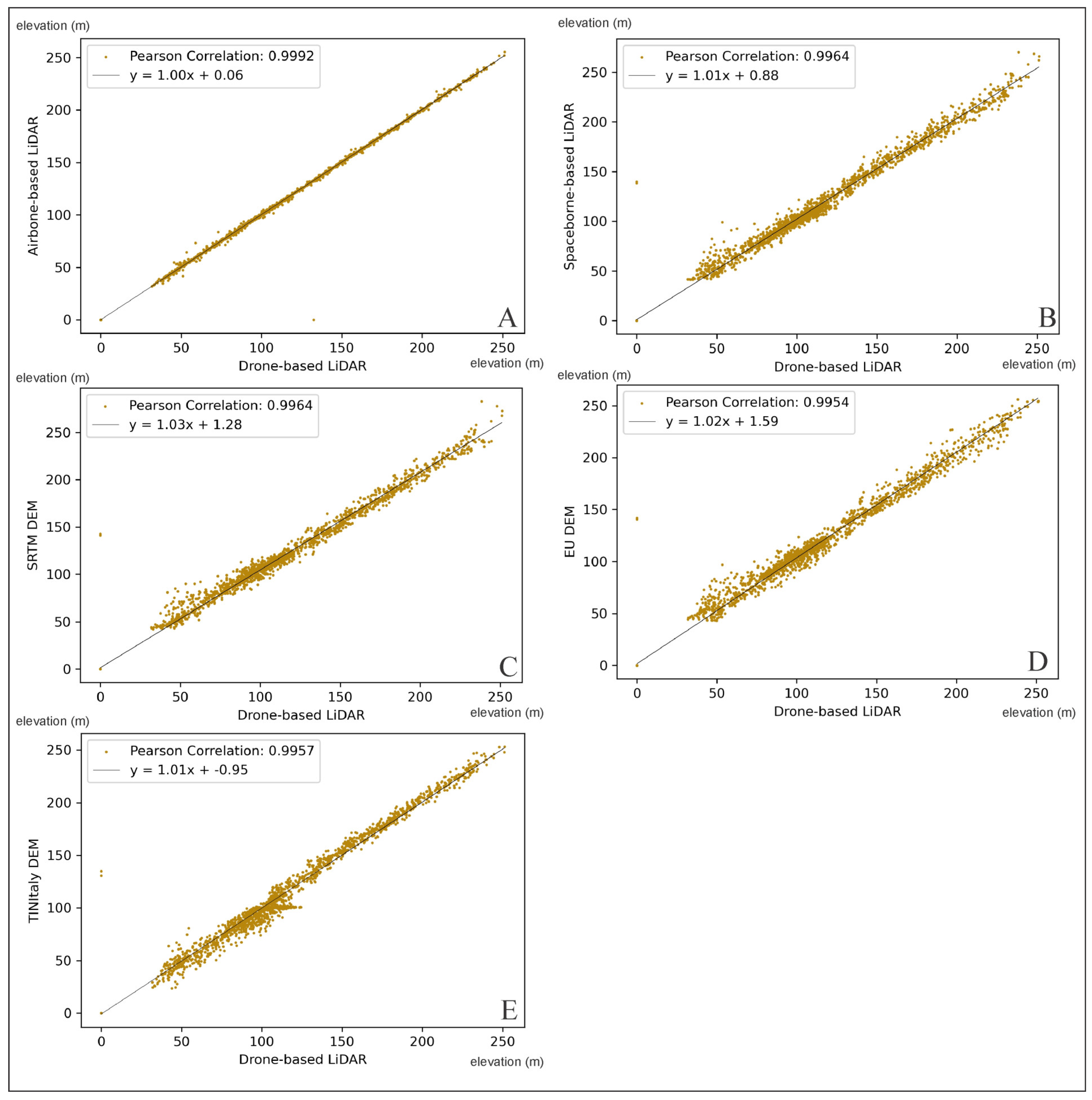
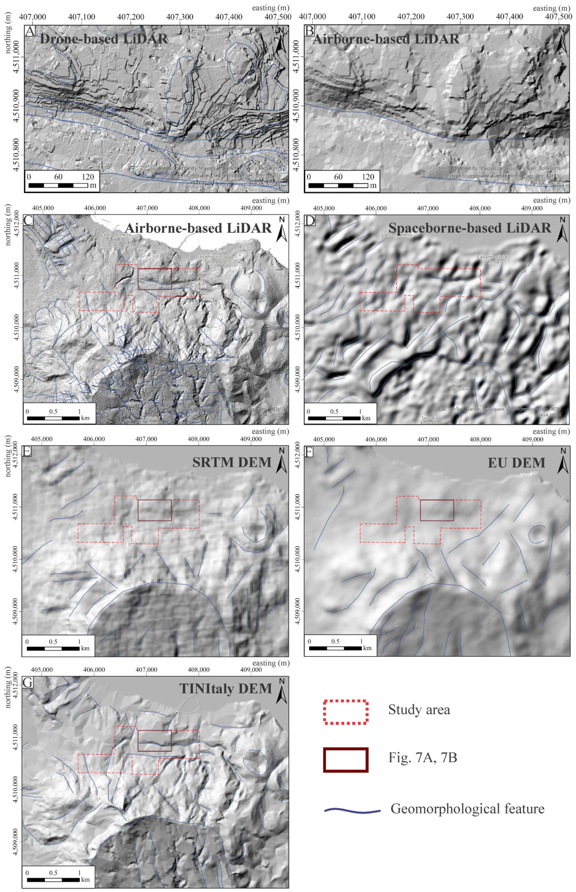
3.4.1. Comparison between Existing Digital Terrain Models Datasets

To evaluate the drone-based LiDAR Digital Terrain Model (DTM), we compared the resolution and the distribution of its elevation values to existing DTMs derived from airborne and satellite-based LiDAR. In the study area, two DTMs derived from LiDAR sensors are currently available:

• The most detailed DTM was obtained through the Italian Extraordinary Remote-Sensing Plan (PST—Piano Straordinario di Telerilevamento). This plan aimed to gather airborne-based LiDAR data and generate a high-resolution DTM product with a 2 m resolution [85].
• On the other hand, a DTM dataset was obtained from the Global Ecosystem Dynamics Investigation (GEDI) instrument, a LiDAR system installed on the International Space Station (ISS). Since its launch in 2018, it has provided high-quality 3D observations over 25 m circular paths on the ground, providing elevation data at 30 m resolution [86].

Additionally, we highlighted the differences between our resulting DTM and the available DTM datasets based on other remote-sensing techniques:

• The Shuttle Radar Topography Mission (SRTM) DTM products are widely regarded as the most comprehensive and highest-resolution freely available data, providing global coverage through radar interferometry. The SRTM data were collected with a sampling grid of approximately 30 m × 30 m [87].
• The EU-DEM v1.0 is a digital surface model (DSM) representing the first illuminated surface as captured by the sensors. This hybrid product combines SRTM and ASTER GDEM data using a weighted averaging approach, resulting in a contiguous dataset divided into 1-degree by 1-degree tiles following the SRTM naming convention [88].
• The 10-m TINItaly DTM serves as a link between the coarse-resolution global SRTM and ASTER DTMs and the emerging very high-resolution airborne LiDAR-based DTMs (such as the mentioned DTM at 2 m resolution) (e.g., [89,90,91]).

The first comparison was based on the calculation of the Pearson correlation coefficient, which measures the strength of the linear relationship between two datasets. We used the resulting DTM as a benchmark to compare its elevation points with those derived from the available DTM dataset above-mentioned (Figure 6). The second analysis involved evaluating shaded relief maps derived from the same DTM datasets. For each DTM, we identified geomorphological lineaments displayed in the shaded relief maps, potentially associated with regional or minor geological structures (Figure 7). This approach facilitated a comparison between the differences and scopes within the same laser system but acquired at different scales and distances.

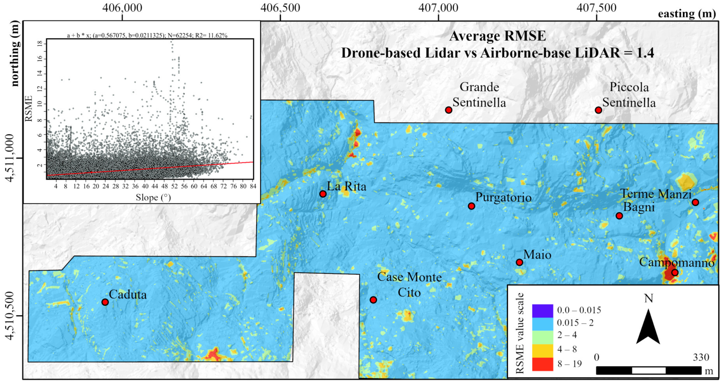
3.4.2. Vertical Accuracy

The vertical accuracy across a DTM elevation’s values primarily assesses the elevation data quality [92]. The absolute vertical accuracy is determined with a Geodetic–Cartographic Reference System that establishes an official datum. This accuracy measure is necessary for large-scale DTM data in provinces, countries, or regions. Given the small extension of our study area, we have not conducted this calculation.

On the other hand, relative accuracy is better for local analyses, especially when additional derived products such as slope and aspect are extracted [93]. To determine the relative accuracy, we compared the differences between our obtained DTM and a known DTM source (referred as DTM_ref). In order to ensure an adequate comparison for similar DTMs derived from LiDAR technology, we used the available PST program’s DTM (2 m resolution) as the benchmark.

It is essential to point out that the term error is inadequate, since the benchmark DTM_ref carries its own uncertainty. Instead, we used the term discrepancy, reserving error solely to denote the original RSME (root square mean error) concept. Since accuracy pertains to the statistical distinction between the assumed accurate DTM (DTM_ref) and the drone-based LiDAR DTM (DTM), the following equations can depict the elevation differences at any given elevation location, the mean of these differences, the standard deviation, and the root mean square error (RMSE):

$${\mathrm{d}}_{\mathrm{i}}={\mathrm{z}}_{\mathrm{D}\mathrm{T}\mathrm{M}}-{\mathrm{z}}_{\mathrm{D}\mathrm{T}\mathrm{M}\mathrm{r}\mathrm{e}\mathrm{f}}$$

(11)

$${\mathsf{\mu }}_{\mathrm{d}}=\frac{1}{\mathrm{n}}\sum _{\mathrm{i}=1}^{\mathrm{n}}{\mathrm{d}}_{\mathrm{i}}$$

(12)

$${\mathsf{\sigma }}_{\mathrm{d}}=\sqrt{\frac{1}{\mathrm{n}-1}\sum _{\mathrm{i}=1}^{\mathrm{n}}{\left({\mathrm{d}}_{\mathrm{i}}-{\mathsf{\mu }}_{\mathrm{d}}\right)}^2}$$

(13)

$${\mathrm{R}\mathrm{M}\mathrm{S}\mathrm{E}}_{\mathrm{d}}=\sqrt{\frac{1}{\mathrm{n}}{\mathrm{d}}_{\mathrm{i}}^2}$$

(14)

where z_DTM is the elevation points of the drone-based LiDAR, z_DTMref is the elevation points of the benchmark DTM, d_i represents the discrepancy in elevation, n the number of samples, μ_d is the mean value of discrepancies, σ_d is the standard deviation of discrepancies, and RMSE_d is the root mean squared error of the discrepancies.

The results derived from Equations (11)–(13) were obtained using the Raster Calculator tool within the ArcGIS Pro 3.0.0 software. The root mean square error (RMSE_d) calculation was transformed into a distribution map to visually identify areas with higher discrepancies and find possible reasons according to the terrain features (Figure 8).

3.5. Derived DTM Products and Morpho-Structural Features Extraction

Structural discontinuities in rock surfaces often express linear features resulting from the intersection between the fault/fractures/stratification planes and the topography. These linear morphologies include linear valleys, ridgelines, and abrupt changes in slope. In order to recognize these elements through a DTM, a lineament is defined by a series of adjacent pixels with similar terrain metrics. Generally, the primary geometric feature to define a single linear expression is the continuity of orientation and length [94]. For normal faults, linear fracture traces depict steep planes (e.g., [95]), and large and elongated areas of uniform aspect and terrain slope with linear boundaries may be associated with surface faulting (e.g., [33,96]).

The linear and areal interpretation and extraction criteria were based on the derivative elevation products (slope, aspect, shaded relief maps) extracted on ArcGIS Pro 3.0.0. The analysis of the slope distribution allowed us to map the linear continuity of this parameter, showing up the presence of scarps, slope breaks, and valleys. On the other hand, the aspect map was used to follow the continuity of crest lines and identify striking changes in scarps. Additionally, the preferential orientation of the surfaces was useful to define the areal distribution of morphological features interpretated as part of different domains. The shaded relief maps helped to distinguish linear features from different contrasts in the images. The delineation of lineaments was enhanced by superimposing the shaded relief map on the slope and aspect maps, verifying the consistency with ridges, valleys, and discontinuities in slopes.

4. Results

4.1. LiDAR Point Cloud

The drone-based LiDAR system acquired 439,643,511 elevation points at 5.8 cm of point separation along 1.27 km² (Figure 3A). The areas covered by each flight and by each strip are summarized in Table 1. For the strips that conformed on each of the five flight missions, there was no mismatch in the planimetric coordinates, meaning that the 3d mismatch was only influenced by z discrepancies and explaining the same values reported in Table 2. The 3d mismatch was slightly reduced after applying a first transformation for each flight line, ranging between 0.74% and 3.53% out of the error. Only one flight showed a significant change of 22.48% over the rest. On the other hand, the 3d transformation for the grouped flights corrected the 3d mismatch between 19.7% and 37.0% (Table 2).

After the ground-filtering process, 16.53% (72,689,631 points) out of the total elevation points were classified as ground points. Different sections across the point cloud showed that the identification of the elevation ground points was efficient in densely vegetated areas (Figure 5). The cross sections located in the Purgatorio area display the capability of our LiDAR laser to register ground points below vegetated areas. This allowed us to identify the presence of a scarp and a counterscarp (Figure 5A,B). Similar results were obtained across the profile located in the Campomanno area, where the presence of vegetation makes it difficult to identify scarp surfaces (Figure 5E,F).

4.2. Digital Elevation Model Quality Assessment

Figure 6 shows the correlation coefficients between the obtained DTM and the available DTMs, along with the scatter plots and regression line equations. Our resulting DTM has a strong correlation value (p = 0.9992) with the airborne-based LiDAR data (Figure 6A), surpassing the accuracy of other available DTMs. Only a few outliers were observed between 50 and 70 m in elevation, with a deviation of 6 cm. This strong correlation suggests that the LiDAR data captured by both the drone- and airborne-based systems were similarly dense, with the possibility that the drone-based LiDAR may have recorded ground points in some areas more effectively than the airborne-based LiDAR.

The details of the shaded relief map revealed that identifying small structures is more challenging and requires additional interpretation compared to the features displayed in the drone LiDAR shaded relief map, despite the already-high resolution level (2 m). This is clearly visible in Figure 7A, where elongated surfaces can be well delineated, and the presence of two canyons can be easily recognized. On the other hand, these features in Figure 7B do not show a clear morphological expression. However, when considering a less-scaled image, a 2 m resolution is sufficient to identify structures on a larger scale (Figure 7B,C).

The correlation between our DTM product and the spaceborne-based LiDAR-DTM is remarkably strong (p = 0.9964). Some outliers deviate by 88 cm, particularly in lower topographic areas ranging from 40 to 70 m in height (Figure 6B). The strong correlation indicates that the spaceborne-based LiDAR and the drone-based LiDAR had a similar data coverage. However, the dispersed outliers can be attributed to the GEDI DTM’s lack of data due to a more extensive spread of LiDAR pulses per area. The derived shaded relief map details reveal a limited exposure of minor structures, suggesting that the application of this DEM dataset is more suitable for morphological analysis at regional scales (Figure 6D).

The correlation between the drone-based LiDAR-DTM and the SRTM-DTM data is notably strong (p = 0.9964). Despite the spaceborne-based LiDAR-DTM and the SRTM-DTM having a similar resolution (Figure 7D,E), a higher elevation offset of 1.28 m exists between the SRTM-DTM and the drone-LiDAR-DTM (Figure 6C). The most dispersed data points are observed between elevations of 45 and 75 m and at higher elevations of around 250 m. The morphological evidence of minor morphological structures is complex to interpret based on the SRTM shaded relief map (Figure 7E). Similar to the GEDI shaded relief (Figure 7D), the application of this data is more proper for regional structural analysis.

A strong correlation is evident when comparing the drone-based LiDAR-DTM with the EU-DEM (p = 0.9954). However, the outliers have the highest offset (1.59 m) compared to other DTM products across the entire area (Figure 6D). The displayed details in the derived shaded relief map are challenging to interpret, even for major structures, because the terrain appears to be very smooth, and it obscures the delineation of the main structures (Figure 7F).

The correlation between the obtained drone-based LiDAR-DTM and the TINItaly-DEM is strong (p = 0.9957) (Figure 6E), slightly lower than the SRTM-DTM but higher than the EU-DEM (Figure 6C,D). The linear regression indicates a negative offset of 0.95 m compared to the obtained drone-based LiDAR-DEM (Figure 6E). The shaded relief derived from this product offers a suitable means to identify both major and minor structures, albeit with some coarse details. The TINItaly-DTM can be an advisable starting point when LiDAR products are unavailable (Figure 7G).

Vertical Accuracy

The computation of Equations (11)–(13) yielded a mean discrepancy value (μd) of 0.44 m and a standard deviation (σd) of 1.34 m. The root mean square error (RMSE) distribution map shows an average value of 1.4 m (Figure 8).

The relatively low values observed for both the mean (μd) and standard deviation (σd) suggest a high level of accuracy in our obtained drone-based LiDAR DTM. Given that the RMSE value is frequently utilized as a parameter to express a DTM’s vertical accuracy, the similarity between the RMSE value and the standard deviation indicates a minimal bias, approaching zero.

As is evident from the scatter plot depicted in (Figure 8), high RMSE values are concentrated in regions characterized by steeper slopes (<48°), commonly corresponding with deep canyons covered by dense vegetation (e.g., Figure 3B,C and Figure 5). In such instances, the observed discrepancies in the RMSE distribution can be attributed to the different capacities of the LiDAR lasers to penetrate vegetated places. The statistical analysis between the drone-based LiDAR and its airborne counterpart exhibits a more remarkable ability to capture bare earth points (e.g., Figure 5).

4.3. Morpho-Structural Analysis

The shaded images, slope, and aspect distribution maps reveal significant areal and linear features. We outlined the key findings derived from the examination of the slope and aspect distribution maps, along with the prominent topographic characteristics identified through the shaded images, perspective views, and topographic profiles.

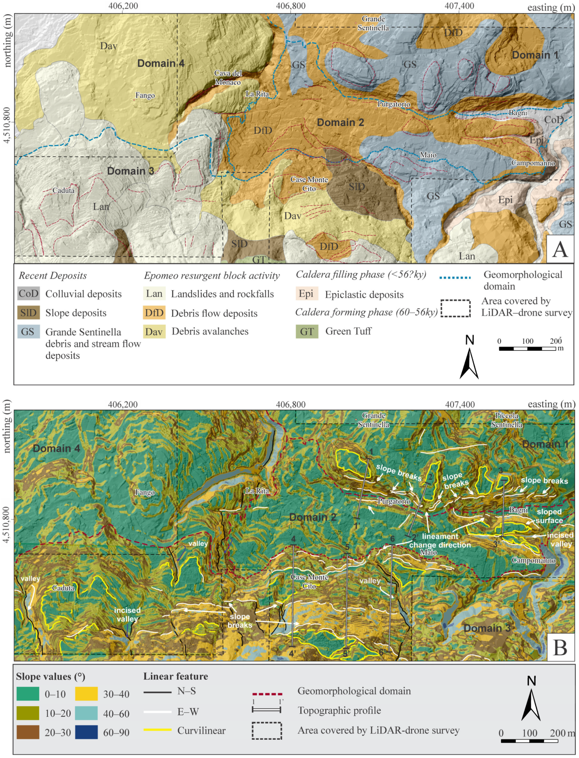
4.3.1. Areal Features

We interpreted the distinctive slope, aspect distribution, and surface textures of the area at the base of Mt. Epomeo to manually divide it into four morphological domains (Figure 9).

Domain 1 is localized in the northernmost part of the study area (Figure 9A,B) and is limited by a continuous change in a slope around the Purgatorio and Bagni latitudes. Elevated, curved, and sloped surfaces are well-identified in the slope map, with slope values lower than 15°; only the borders of these surfaces show a few slopes up to 30°. In the aspect map, they show a radial and multi-directional distribution of aspect classes (Figure 9C). The surfaces to the west and east of the Purgatorio zone coincide, having a maximum height of 125 m (Profiles 1 and 2 in Figure 10), whereas the surfaces to the easternmost part show a height between 95 and 110 m a.s.l. (Profile 3 in Figure 10). According to the shaded relief map, these features correspond with terraced morphologies in which sand and silty sand deposits have covered the areas during the most recent debris and stream flow events (Figure 9A). The rest of the domain is characterized as moderately fragmented in slopes. The areas with abrupt changes in slope coincide with the contact between recent debris and stream flow deposits and older debris flow and landslides deposited during the resurgent activity of the Mt Epomeo block (Figure 9A). The areas where the recent deposits are reported (Figure 9A) show a variable change in the direction of the surfaces, resulting in a rough texture revealed on the aspect map (Figure 9C).

Domain 2 is localized in the central part of the study zone (Figure 9A); it is limited to the north by the well-defined breaks in slope from the Purgatorio to the Bagni area (Figure 9B), and to the west by a N-S-sloped surface. Most of 50% of this domain shows minor slope changes (Figure 9B). This coincides with the deposition of ancient debris flow and landslides from the Epomeo resurgent block activity (Figure 9A) that, like in Domain 1, do not show any trend of orientation surface (Figure 9C). To the east of the domain, the surfaces show a sharp slope break (between 45° and 60°). In this area is also visible the presence of an elevated and E-W-elongated area between 70 and 75 m in height (Profile 3 in Figure 10), with a relatively flat top dissected by an E-W incised valley (Figure 9B). Ancient debris flow, landslides, and rockfalls were deposited, whereas epiclastic deposits filled the lower valley in the Campomanno area (Figure 9A).

Domain 3 is localized in the southern area (Figure 9A,B). This domain presents a morphology with numerous slope breaks belonging to the northern flank of Mt. Epomeo. The slopes are very steep, with changes up to 50°. Unlike the previously described areas, the distribution of aspect classes shows a general inclination to the N and NE. Some N-S shallow valleys dissect the sloped surfaces (Figure 9B). This domain is covered mainly by deposits of landslides, rockfalls, and avalanches that originated during the Holocene uplift phase of the Mt Epomeo resurgent block (Figure 9A). Similar to domains 1 and 2, continuous slope values characterize elongate and planar surfaces, which, according to the shaded relief views, can be attributed to the presence of step-like landforms (Figure 9A). The top height of these landforms ranges between 175 and 185 m in the western part of the domain, near the Caduta area, and between 145 and 130 m for the surface near the Case Montecito and Maio sites, respectively (Profiles 4 and 6 in Figure 10).

Domain 4 is in the north-westernmost part of the study area (Figure 9A,B). Its limit is characterized by a sharp change in slope, defining a N-S surface that coincides with domain 2. The presence of a deep valley is evident by the abrupt change in slope and marked by the aspect class defining both sides of the canyon (Figure 9B,C). Around the Cava del Monaco area, the surface is characterized by constant slope values with minor slope breaks along a continuous curve.

4.3.2. Linear Features

The morphological analysis reveals many linear features visible as rectilinear or curvilinear topographic traces. These were characterized by the continuity of the same slope values along a surface, a dominant aspect class, the density of the same striking direction, and changes in the slopes (slope breaks) located at the same elevation.

In the southern limit of domain 1, slightly to the north of the Purgatorio area, the slope breaks define the contour of surfaces with gentle angles (<10°) to steeper ones between 20° to 30°. These surfaces follow slightly WNW lineaments along 200 m from the west of the Purgatorio site to the east (Figure 9B). Along this sector, the aspect map shows a change in the direction of the sloped surfaces from SW to SE (Figure 9C). The striking direction of the lineaments changes towards ENE along 1 km to the east, near the Bagni zone. In this portion, the orientations change slightly from S to SE, defined by the change in aspect class (Figure 9B,C). According to the extracted topographic and slope profiles crossing the described linear features, the main slope break occurs between 110–111 m (Profiles 1 and 2 in Figure 10) and 90 m (Profile 3 in Figure 10). The changes in the slope values range between 11° and 45° and are limited by the terraced landforms previously described for domain 1 (Profiles 1–3 in Figure 10).

Eighty meters to the south of the limit between domains 1 and 2, a slope surface runs parallel to the previously described WNW structure. This extends 250 m to the SE, to then change abruptly from steep to moderate angles, forming an S-shape sloped lineament along 340 m to the E (Figure 9B). The aspect map shows a change in the inclination of these surfaces from N and NE. A semi-continuous line between these parallel WNW-ENE slopes leads to defining it as a counterslope (Figure 9C). The topographic profiles show that the main breaks in slope occur at 96, 106, and 67 m in height, with changes in slope between 34° and 40°. The analysis in the shaded relief map shows a narrow valley formed by the described WNW-ENE sloped surfaces identified as linear features. The details in the shaded relief map allowed us to define the bottom of the depression formed between the previous lineaments (Figure 7A and Figure 9A). In the limit between domain 4 and domain 2 is visible an N-S-striking lineament that changes abruptly to E-W and to N-S in the La Rita area (Figure 9B).

To the north of Case Monte Cito and Maio, between domains 2 and 3, a series of moderate steep surfaces define an S-curved lineament (Figure 9B). The main strike direction of these slopes is E-W (Figure 9B), dipping towards the NW (Figure 9B). These lineaments run at the base of the terraced surfaces described in the previous section. As shown on the topographic profiles, the main slope breaks coincide at a height of 113 and 125 m (Profile 4–6 in Figure 10).

Many slope breaks characterize the south part of domain 3; the surfaces show very steep angles defining E-W-striking lineaments (Figure 9B). Notably, the continuity of slopes with the same changes in their values is almost constant at heights between 201 and 211 m (Profiles 4–6 in Figure 9), with a dominant inclination northward (Figure 9C). Steep-sloped surfaces (from 30° to 45°) define N-S lineaments cutting the E-W linear features; these surfaces generally dip towards the W (Figure 9C). The shaded relief map shows that both lineaments define the Mt. Epomeo front (Figure 9A).

5. Discussion

5.1. Data and Digital Elevation Model Quality

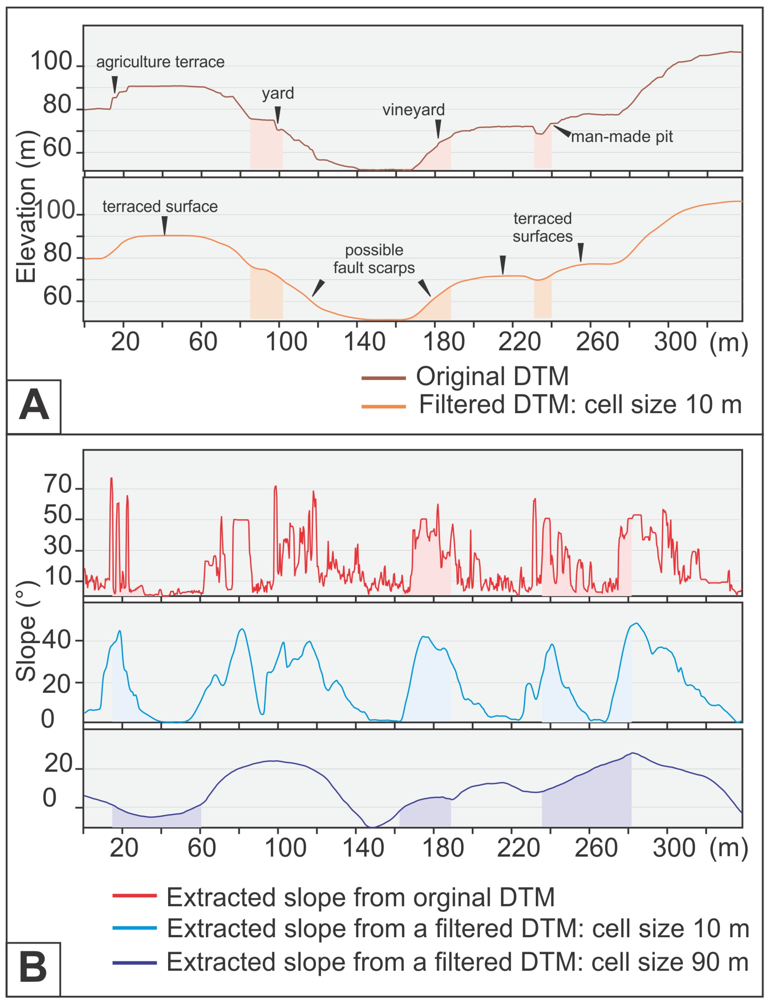
The applied workflow effectively reduces systematic errors in the raw drone LiDAR data, as outlined in Table 1. While the initial LiDAR data displayed an acceptable accuracy in planimetric (xy-coordinates) and elevation (z-coordinate) measurements, the systematic error correction process significantly enhanced the precision of the LiDAR data. By implementing the 3D-strip adjustment step, we minimized the RMSE between flight lines between 0.04 and 0.06. These low RMSE values ensure less probability of wrong features such as disjointed lines, false ridges, or inconsistencies along flight borders. These improvements are relevant to prevent the identification and misinterpretation of geomorphological characteristics.

Our findings established a strong and linear correlation with the existing DTMs for the same geographical region. Elevation data extracted from LiDAR sensors and acquired through various platforms exhibit the most robust correlation coefficients. This feature can be ascribed to the capacity of LiDAR laser technology to acquire precise ground elevation points in vegetated areas, surpassing photogrammetric techniques in which the vegetation is removed by estimating its height above the ground [2,11,97]. The observed spread and deviation in elevation values within our results can be attributed to a larger volume of data elevation points for a specific area, in contrast to fewer data points captured by alternative methods over the same region.

5.2. DTM Resolution

The obtained DTM shows a very high detail so far for the study area compared to previously available DTMs. Our results significantly improved the identification of minor details in faulting structures (Figure 7A and Figure 9) through geomorphological features. Hillshades derived from coarser DTMs (Figure 7D–G) do not clearly display local structures, making any interpretation of faulting structures impossible. However, determining the appropriate DTM data resolution for terrain-based modeling depends on the research interest and scope. A common challenge is that the grid DTMs tend to be oversampled in low-relief areas, while being under-sampled in high-relief regions [98].

One effective approach to enhance terrain detail representation involves increasing the sample point density, while reducing the grid size. Thus, we selected a DEM grid (20 cm) coarser than the data point density (5.8 cm). This was suitable for the complex topographic terrain, encompassing hills and plains, and the required detail to identify active deformation features.

The accuracy and density data of the first derivative products, such as slope and aspect maps, were significantly impacted by the presence of minimal elevation values in adjacent pixels, attributed to anthropic influences like vineyards, houses, and roads (Figure 11). To extract morphological information and reveal geological structures across different scales without the influence of non-natural landforms, we applied a smoothing filter process for the resulting DTM. We utilized a 10 m × 10 m mobile window and applied mean filtering through the Focal Statistics tool in the ArcGIS Pro 3.0.0 software. Figure 11 shows how elevation and slope profiles extracted from the raw DTM display a very detailed profile. However, the data density captured by the laser beam also yielded high-frequency elevation variations. Thus, the application of a smoothing filter was necessary to extract only the evidence of morphological features. In this way, the terrain features became more prominent and easily interpretable, as depicted in the filtered profiles in Figure 11B.

5.3. External Factors Consideration for DTM Accuracy and Reliability

The application of drone-based LiDAR entails different factors to consider when this tool is used. In this section, we delve into how external conditions of the area influenced both data acquisition and subsequent data treatment. These factors play a remarkable role in the presence of data artifacts in the LiDAR point cloud, which, in turn, influence the reliability and quality of the derived elevation products.

Vegetation. Most parts of Ischia Island are vegetated by Maquis shrubland, dense broad-leaved shrubs, bushes, and small trees typical of Mediterranean latitudes (Figure 3C). Despite the ability of LiDAR technology to penetrate vegetation, these dense and closed-packed forest floors reduce the possibility of the laser beam reaching the ground, resulting in data voids and gaps. Even with advanced ground filters and interpolation algorithms, the final DTM may lack accuracy and lose rugged details. A possible alternative to this issue could be to conduct the LiDAR mapping during the leaf-off season.

Altitude. The choice of flying altitude might be based on different conditions such as the desired area to cover or the flight altitude restrictions. Opting for higher altitudes results in covering larger areas, but it will also increase the incident angle of the laser beam at the swath edges. This, in turn, will reduce the backscattered laser power and will lead to a greater mismatch in the overlapping strips. As presented in Section 3.2.2, the strip calibration can significantly reduce the artifacts in adjacent strips. However, in the case of substantial mismatches, more iterations may be necessary to calibrate the LiDAR data, requiring additional 3D transformation of the LAS (.las) dataset and causing an imminent modification in the original data.

GNSS receiver. The accuracy of georeferencing LiDAR data relies highly on the availability and quality of the GNSS receiver. Accuracy diminishes with the distance from the GNSS receiver, highlighting the importance of having the base station close to the take-off point. In such scenarios, employing a mobile GNSS receiver, free from coverage interference, is recommended to achieve better results. Alternatively, when GNSS receiver usage is not feasible, the use of a Continuously Operating Reference Station serves as a viable alternative.

Point cloud filtering algorithm. While the applied ground filter algorithm demonstrated an efficient performance, the available ground-filtering methods operate on different surface parameters. Our study found that employing a two-iteration filtering process adequately captured ground points in areas with high slopes due to the mountain front or along canyons. However, it is possible that, for less sloped terrains, a single iteration may be enough, or for regions with a more rugged topography, an alternative algorithm based on different filter functions might be necessary.

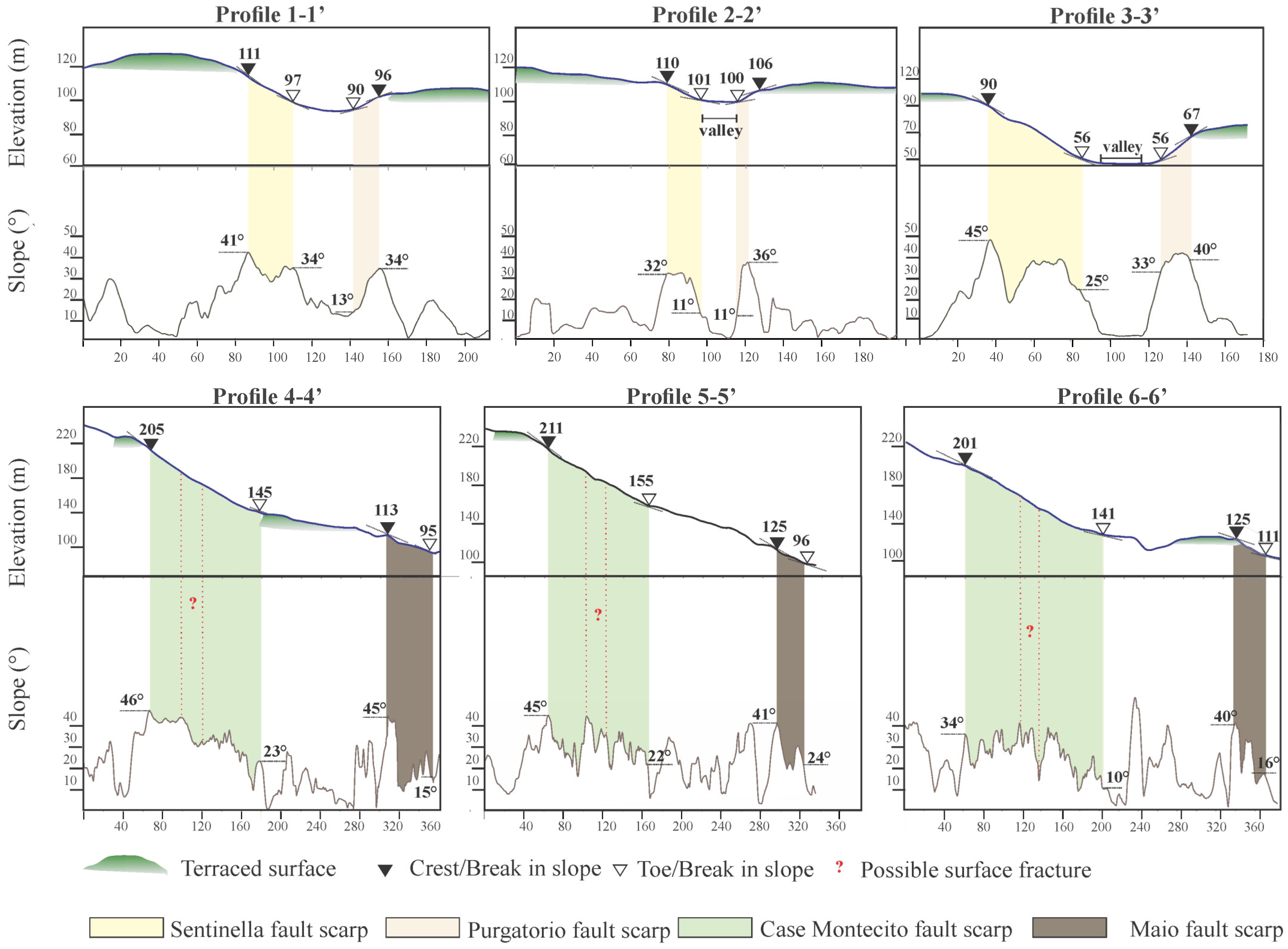
5.4. Definition of Fault Scarp Structures

While previous studies have documented the existence of a Holocene graben structure in the piedmont area to the north of Ischia Island [25,30,32], our outcomes have permitted the identification and quantification, as much as possible, of similar morphological features along various segments of the faults. Through this approach, we have attained more precise delineations of fault trace geometries and identified additional faulting structures previously unreported (Figure 12). The analysis of scarp morphology was based on topographic and slope profiles (Figure 10) and the final definition of fault traces is presented in Figure 12.

Considering that the development of the fault structures dates back to ca. 33,000 years, during the earliest phase of the Mt Epomeo block uplift [25], factors such as gravitational activity, rain-induced material transport, faulting processes, and the mechanical properties of the rock have played significant roles in influencing erosion rates along the fault scarps, leading to the degradation of morphometric elements [99]. Nevertheless, the identified slope breaks proved essential indicators for mapping fault scarps.

The presence of terraced surfaces with slight variations in slope and predominantly located at the same elevation (Figure 9 and Figure 10) served as the initial geomorphic marker for identifying the original rupture surface. Gradual slope breaks at the base of these surfaces indicate the upper part or crestal zone of the scarp [99,100]. Along this crestal area, the surface exhibits a rounded and convex upward profile (Figure 10). Even though a non-continuous crestal zone was displayed on the morphological features (Figure 9B), various dissected slope breaks were evident. Another element of the fault scarp identified by a slope break and belonging to the lowest part of the scarp was the base or toe [99,100]. Similar to the crestal part, the identification of the scarp toes was guided by their appearing at consistent heights. Additionally, the shaded relief map clearly illustrates the toes of the scarps (Figure 7A and Figure 9A), facilitating their delineation.

In the subsequent sections, we delve into the geomorphic features and geometry of the fault scarps that constitute the CHG and the E-W master fault segment in the northern flank of Mt. Epomeo.

5.4.1. Maio Fault: Southern Synthetic Fault

Along the boundary between morphological domains 2 and 3, the scarp of the Maio fault is characterized by crestal and toe zones ranging from 125 m at its maximum height to 96 m at the lowest point (Profiles 4–6 in Figure 10). The slope values exhibit high inclination angles (reaching up to 45–40° and 15–24° for the crests and the toes, respectively), with an average intermediate slope of 26° (Profiles 4–6 in Figure 10). These values show a possible debris- and wash-controlled degradation process [100]. The horizontal length of the scarps vary, with the longest extending up to 70 m and the widest reaching approximately 20 m. Notably, this scarp changes strike direction, from ENE-WSW in the western segment to WNW-ESE in the eastern segment, defining an S-shaped trace dipping to the NNE and to the NNW, respectively (Figure 9B,C and Figure 13).

5.4.2. Sentinella Fault: Northern Antithetic Fault

Between morphological domains 1 and 2, the Sentinella fault is the antithetic structure of the CHG. The elevations for the crestal areas range between 90 m and 115 m, slightly lower heights than the Maio fault. The scarp also exhibits low slope angles, ranging between 45–32° and 11–34° for the crests and the bases, respectively, with average intermediate slopes of 26°. These values are indicative of an erosion controlled by debris and wash processes [100]. In the western sector, the fault strikes from WNW-ESE to ENE-WSW, dipping to the S-SW and further to the SE in the eastern segment. One possible explanation for this change in strike between the Maio and the Sentinella faults might be the presence of a NE-SW structure (Figure 12; and profiles 3 and 4 in Figure 13) associated with the NE-striking faults reported by Tibaldi et al. (1998) [30] to the N part of the island.

This structure could be reactivated during different inflation and deflation cycles of the caldera or during other earthquakes events, influencing the S-shape of the E-W-striking faults and tilting the foothill slightly to the E-SE, most visible in the northern horst of the CHG (Figure 9C, profile 4 in Figure 13).

5.4.3. Monte Cito Fault: Master Fault

At the base of Mt. Epomeo, similar slope values break along a similar elevation (201–211 m, Figure 9B, profiles 4–6 in Figure 10). The crest areas are present between 201 and 211 m, whereas the toes are between 140 and 155 m. The slope surface undergoes average steep angles around 32°, with 34°, 45°, and 46° values for the upper crest, with 10° and 23° for the bases. These slope values are likely attributed to debris-controlled processes of scarp degradation [99,100]. The strike changes in its western portion from ENE-WSW to WNW-ESE and defines an S-shaped trace similar to the previous faults. Topographic and slope profiles reveal varying slopes along the scarp. This observation suggests the possible existence of intermediate surface ruptures as a result of distinct earthquakes and possibly reflected in the presence of composite fault scarps (e.g., [101,102]) (Profiles 4–6 in Figure 10).

The western segment shows the narrowest part of the graben, about 250 m, with a topographic depth of 20 m. The northern and southern marginal shoulders reach an elevation of 80 and 100 m, respectively. On the other hand, the eastern part of the CHG is wider, 370 m in size and with a topographic depth around 40 m; the marginal shoulders reach an elevation of 80 m to the south and 97 m to the north.

5.5. Structural and Geological Control on Morphology Features

A critical analysis of the relationship between the geomorphological features, the origin and distribution of Quaternary deposits and the slip rates of the active faults, points out the dominant role of each factor over the landscape’s evolution. Based on the stratigraphic correlation between the sediments that form the terraced surfaces and their presence in drillholes at the interior and exterior of the CHG, as well as its constraining by dated lava deposits, Michetti et al. (2023) [103] have estimated a cumulative slip rate of 26 mm/yr and 6 mm/yr for the Monte Cito and Sentinella faults, respectively. These high values can be correlated with high vertical erosion rates [102], explaining the presence of steeper slopes in the scarp of the Case Montecito fault in comparison to the slopes along the Sentinella fault scarp (Figure 9B and Figure 10).

Additionally, the mechanical properties and depositional processes of the rocks are factors that strongly control the surface evolution. The southern part of the area is dominantly covered by epiclastic deposits after the recent uplift phase of the Mt Epomeo block [42,45]. As a result of the rapid uplift, high erosion rates triggered edifice collapses and generated debris avalanches, landslides, and rockfalls deposits (Figure 9A). The preferential orientation of the slopes that developed on the areas covered by these deposits (Figure 9C) is parallel to the transport direction of the material (N and NE). However, in their most distal locations, the deposits are distributed with random orientations (morphological domain 1 in Figure 9A,C). The abrupt and chaotic origin of these deposits caused very poorly classified and pervasive fractured block-facies material or completely shattered debris–avalanche blocks. This is reflected in sharp and high sloped surfaces near the border of Mt. Epomeo (Figure 9B and Figure 10).

The resurgence events of the Mt. Epomeo block triggered phases of uplift and destabilization, originating debris and mudflows events. Earthquakes, on the other hand, led to the formation of landslide deposits [44] (Figure 9A) filling the graben depression. The high erosive dynamics of the drainage systems are highly controlled by the rapid fault slip rates and might facilitate a downcutting erosion process well-observed by the presence of terraces in the interior of the CHG (Figure 10). The smooth terrain surfaces in the graben depression (morphological domain 2) (Figure 9) suggest a strong influence on the morphology controlled by the deposition of sediments transported from the footwalls (Figure 9A).

6. Conclusions

The main achievements of this study can be summarized as follows:

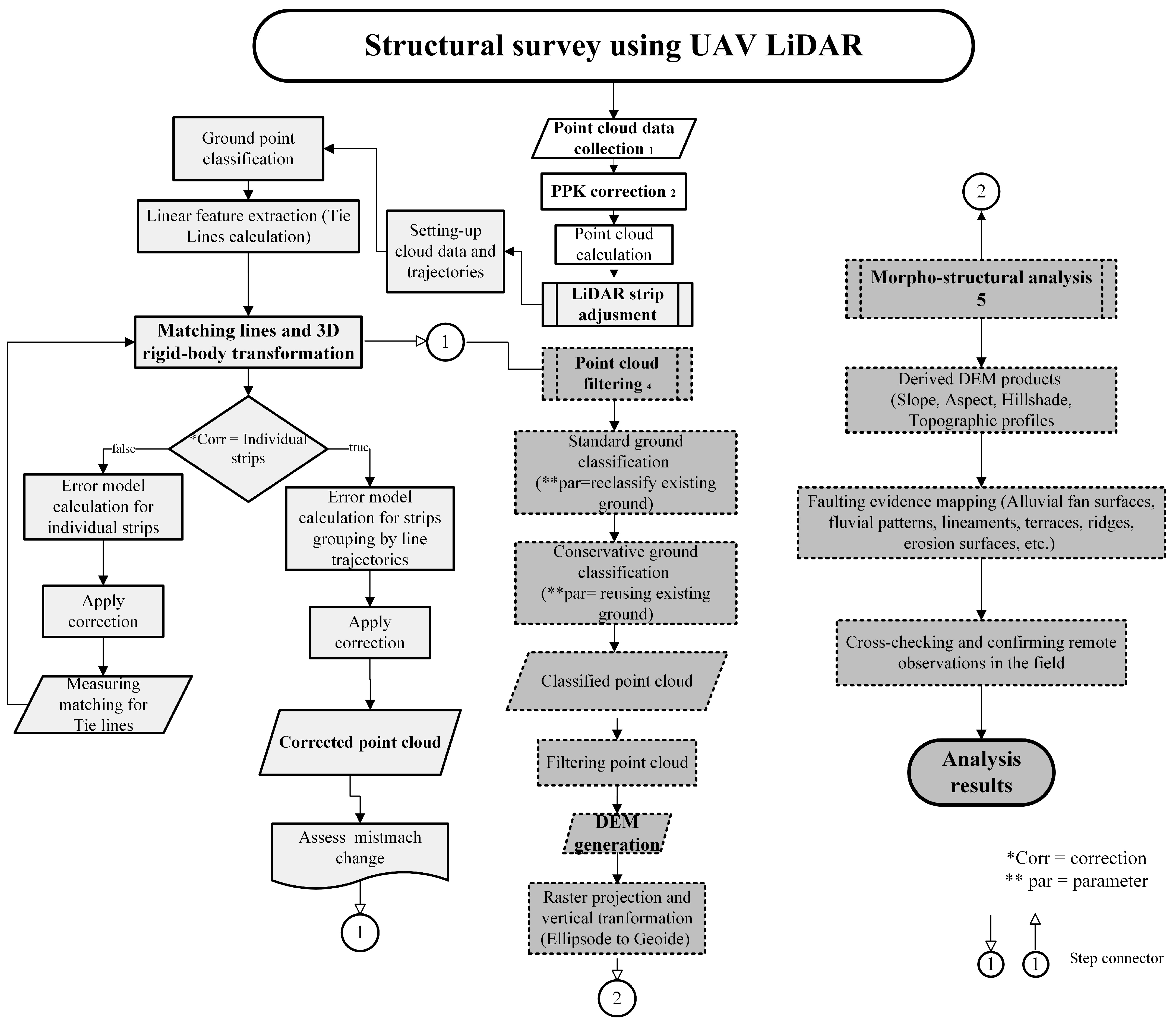
• Although the presented workflow (Figure 4) implies different processes commonly applied for the usage of LiDAR data, we proposed a novel application of drone-based LiDAR data adapted to show accurate and precise geomorphological information. A similar approach can be used in areas where the evidence of high deformation rates is masked by vegetation conditions or by inaccessible areas. Particularly, the 3D transformation process to calibrate the point cloud raw data improved the quality of the DEM data and its subsequent derived products. The mismatch that existed has been reduced, avoiding the effect of artifacts in the elevation data products.
• The approach for the ground-filtering process showed an acceptable classification between the ground and non-ground control points. The verification through the analysis of cloud point profiles and the control fieldwork led us to consider the ground-filtering process accurate enough to preserve the ground points captured by the LiDAR laser beam.
• The drone-based LiDAR outcomes yielded the most accurate and detailed Digital Elevation Model for the northern part of Ischia Island. However, compared to existing DEM datasets, our result is the first DEM able to display evidence of active deformation.
• The northern flank of Mt. Epomeo is characterized by four different morphological domains revealed by the linear and areal features extracted from the drone-based LiDAR. The characteristic of each domain has been the result of the interplay between the (1) the deposition mechanics and the sedimentological properties of the covering rocks, (2) the active faulting developed throughout the resurgence history of Mt. Epomeo, (3) different slip rates, and (4) erosion and deposition processes.
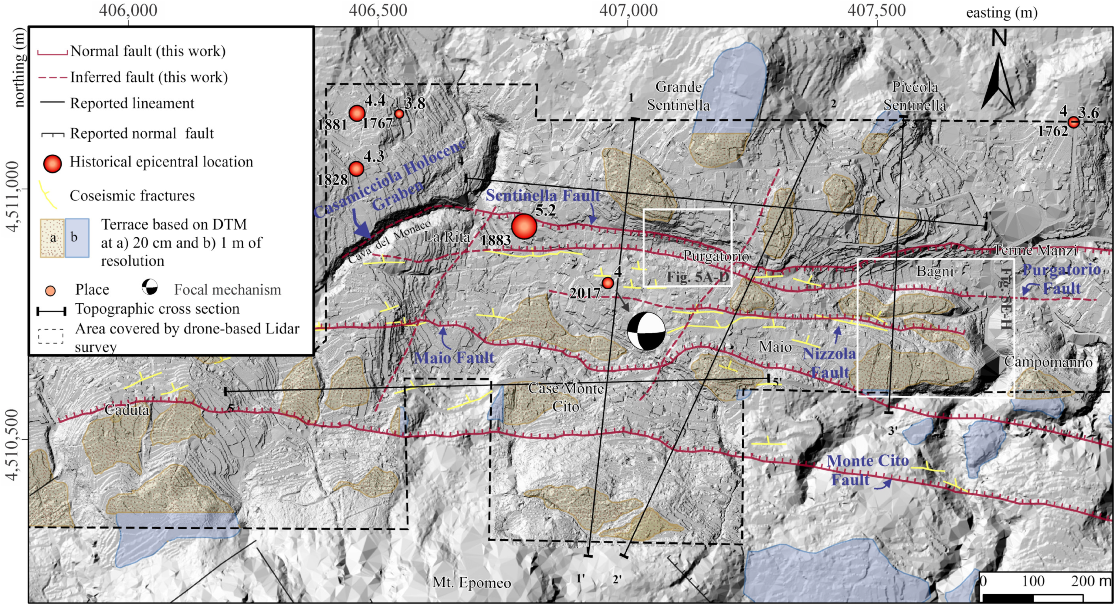
• The identification of terraced surfaces, slope breaks, scarp toes, and their morphometric values, their corroboration on the field, and morphological features previously unreported, allowed us to define a detailed geometry of the fault structures in the CHG. To the southern part of the Casamicciola Holocene Graben (CHG), the E-W-striking Monte Cito fault represents the master structure (Figure 12). The southernmost and synthetic structure (Maio fault) that forms the CHG runs at the base of different terraced surfaces at a maximum height of 125 m. The northernmost and antithetic fault structure is well-defined at the base of terraces at 115 m. Both faults coincide with the previously inferred main structures by Tibaldi and Vezzoli (1998) [30].
• The evolution of the northern flank of Mt. Epomeo, in combination with the fastest slip rate (26 mm/yr), shows a major control on the morphological features along the southern faults of the CHG. In contrast, the northern horst structure is morphologically more controlled by a lower slip rate (6 mm/yr), whereas the central part of the graben has been modified by the processes of erosion/sedimentation and deposition, rather than faulting activity.
• Our research shows the remarkable efficacy of drone-based LiDAR in neotectonic mapping. The identified geomorphological features were indispensable for characterizing and interpreting the presence of active faults and the analysis of landscape morphology and its relationship with geological evolution. Additionally, the technique speeded up time-consuming mapping tasks, while facilitating access to challenging areas at affordable prices.
• The potential applications of drone-based LiDAR extend far beyond our specific study, being applicable across different geological environments. In paleoseismological studies, high-resolution DTMs can serve as guidance for an accurate identification of trenching sites. A precise and detailed mapping of drainage patterns and gullies can lead the location of fault surface exhumation, while avoiding areas affected by erosional processes. Additionally, detailed morphological data enhance the accuracy of quantifying landform offsets and fault displacements, important for the reconstruction of past seismic events. Furthermore, this tool can also assist in the characterization of volcanic activity mechanisms and their influence over the flow dynamics, rheology, and morphology emplacement of volcanic materials (e.g., lahars, pyroclastic density currents, tephra fall). This is particularly important when emplacement and collapse mechanisms, and cover distribution and extension, are considered to produce volcanic risks scenario maps. Additionally, assessing volcanic hazards often involves the modeling of past volcanic flows, where the drone-based LiDAR can represent probably one of the best sources to produce trustworthy DTMs to obtain confident simulation results. Drone-based LiDAR products can be essential also in the study of sedimentary basins, where the morphological characterization of fluvial fans sheds light on understanding paleoclimate and tectonic signals, as well as concerning geological hazards. Lastly, in civil engineering planning, this tool can be useful in areas where vegetation may obscure morphological evidence of unstable slopes, fault structures, shear zones, caves, karstic sinkholes, etc. In this way, engineering plan projects can mitigate risks, optimize designs, and ensure the long-term stability and safety of infrastructure.

References

1. Shan, J.; Hyyppä, J. Advances in Airborne Lidar Systems and Data Processing; CRC: Boca Raton, FL, USA, 2018. [Google Scholar]
2. Baltsavias, E.P. Airborne laser scanning: Existing systems and firms and other resources. ISPRS J. Photogrametry Remote Sens. 1999, 54, 164–198. [Google Scholar] [CrossRef]
3. Mazzarini, F.; Pareschi, M.T.; Favalli, M.; Isola, I.; Tarquini, S.; Boschi, E. Morphology of basaltic lava channels during the Mt. Etna September 2004 eruption from airborne laser altimeter data. Geophys. Res. Lett. 2005, 32, 1. [Google Scholar] [CrossRef]
4. Mouginis-Mark, P.J.; Garbeil, H. Quality of TOPSAR topographic data for volcanology studies at Kilauea Volcano, Hawaii: An assessment using airborne lidar data. Remote Sens. Environ. 2005, 96, 149–164. [Google Scholar] [CrossRef]
5. Davila, N.; Capra, L.; Gavilanes-Ruiz, J.C.; Varley, N.; Norini, G.; Vazquez, A.G. Recent lahars at Volcán de Colima (Mexico): Drainage variation and spectral classification. J. Volcanol. Geotherm. Res. 2007, 165, 127–141. [Google Scholar] [CrossRef]
6. Ventura, G.; Vilardo, G. Emplacement mechanism of gravity flows inferred from high resolution Lidar data: The 1944 Somma-Vesuvius lava flow (Italy). Geomorphology 2008, 95, 223–235. [Google Scholar] [CrossRef]
7. Favalli, M.; Fornaciai, A.; Pareschi, M.T. LIDAR strip adjustment: Application to volcanic areas. Geomorphology 2009, 111, 123–135. [Google Scholar] [CrossRef]
8. Kósik, S.; Németh, K.; Rees, C. Integrating LiDAR to unravel the volcanic architecture and eruptive history of the peralkaline Tūhua (Mayor Island) volcano, New Zealand. Geomorphology 2022, 418, 108481. [Google Scholar] [CrossRef]
9. Neri, M.; Mazzarini, F.; Tarquini, S.; Bisson, M.; Isola, I.; Behncke, B.; Pareschi, M.T. The changing face of Mount Etna’s summit area documented with Lidar technology. Geophys. Res. Lett. 2008, 35, 1–6. [Google Scholar] [CrossRef]
10. Conforti, M.; Mercuri, M.; Borrelli, L. Morphological changes detection of a large earthflow using archived images, lidar-derived dtm, and uav-based remote sensing. Remote Sens. 2021, 13, 120. [Google Scholar] [CrossRef]
11. Liu, X. Airborne LiDAR for DEM generation: Some critical issues. Prog. Phys. Geogr. 2008, 32, 31–49. [Google Scholar]
12. Dong, P.; Chen, Q. LiDAR Remote Sensing and Applications; CRC Press: Boca Raton, FL, USA, 2018. [Google Scholar]
13. Schroder, W.; Murtha, T.; Golden, C.; Scherer, A.K.; Broadbent, E.N.; Almeyda Zambrano, A.M.; Herndon, K.; Griffin, R. UAV LiDAR survey for archaeological documentation in Chiapas, Mexico. Remote Sens. 2021, 13, 4731. [Google Scholar] [CrossRef]
14. Resop, J.P.; Lehmann, L.; Cully Hession, W. Drone laser scanning for modeling riverscape topography and vegetation: Comparison with traditional aerial lidar. Drones 2019, 3, 35. [Google Scholar] [CrossRef]
15. Arora, K.; Srinu, Y. Surface traces of seismogenic faults from airborne LiDAR in Koyna–Warna region of Deccan Volcanic Province. J. Earth Syst. Sci. 2022, 131, 148. [Google Scholar] [CrossRef]
16. Finley, T.; Salomon, G.; Nissen, E.; Stephen, R.; Cassidy, J.; Menounos, B. Preliminary Results and Structural Interpretation from Drone Lidar Surveys over the Eastern Denali Fault; Yukon Geological Survey: Whitehorse, YT, Canada, 2022.
17. Fleming, C.; Marsh, S.H.; Giles, J.R.A. Introducing elevation models for geoscience. Geol. Soc. 2022, 345, 1–4. [Google Scholar] [CrossRef]
18. Valkanou, K.; Karymbalis, E.; Papanastassiou, D.; Soldati, M.; Chalkias, C.; Gaki-Papanastassiou, K. Assessment of Neotectonic Landscape Deformation in Evia Island, Greece, Using GIS-Based Multi-Criteria Analysis. ISPRS Int. J. Geo-Inf. 2021, 10, 118. [Google Scholar] [CrossRef]
19. Barreca, G.; Corradino, M.; Monaco, C.; Pepe, F. Active Tectonics along the South East Offshore Margin of Mt. Etna: New Insights from High-Resolution Seismic Profiles. Geosciences 2018, 8, 62. [Google Scholar] [CrossRef]
20. Vitale, S.; Isaia, R. Fractures and Faults in Volcanic Rocks (Campi Flegrei, Southern Italy): Insight into Volcano-Tectonic Processes. Int. J. Earth Sci. 2014, 103, 801–819. [Google Scholar] [CrossRef]
21. Norini, G.; Groppelli, G.; Sulpizio, R.; Carrasco-Núñez, G.; Dávila-Harris, P.; Pellicioli, C.; Zucca, F.; De Franco, R. Structural Analysis and Thermal Remote Sensing of the Los Humeros Volcanic Complex: Implications for Volcano Structure and Geothermal Exploration. J. Volcanol. Geotherm. Res. 2015, 301, 221–237. [Google Scholar] [CrossRef]
22. Norini, G.; Carrasco-Núñez, G.; Corbo-Camargo, F.; Lermo, J.; Rojas, J.H.; Castro, C.; Bonini, M.; Montanari, D.; Corti, G.; Moratti, G.; et al. The Structural Architecture of the Los Humeros Volcanic Complex and Geothermal Field. J. Volcanol. Geotherm. Res. 2019, 381, 312–329. [Google Scholar] [CrossRef]
23. Tibaldi, A.; Romero Leon, J. Morphometry of Late Pleistocene-Holocene Faulting and Volcano tectonic Relationship in the Southern Andes of Colombia. Tectonics 2000, 19, 358–377. [Google Scholar] [CrossRef]
24. Nappi, R.; Alessio, G.; Gaudiosi, G.; Nave, R.; Marotta, E.; Siniscalchi, V.; Civico, R.; Pizzimenti, L.; Peluso, R.; Belviso, P.; et al. The 21 August 2017 Md 4.0 Casamicciola Earthquake: First Evidence of Coseismic Normal Surface Faulting at the Ischia Volcanic Island. Seismol. Res. Lett. 2018, 89, 1323–1334. [Google Scholar] [CrossRef]
25. Nappi, R.; Porfido, S.; Paganini, E.; Vezzoli, L.; Ferrario, M.F.; Gaudiosi, G.; Alessio, G.; Michetti, A.M. The 2017, md = 4.0, casamicciola earthquake: Esi-07 scale evaluation and implications for the source model. Geosciences 2021, 11, 44. [Google Scholar] [CrossRef]
26. Sbrana, A.; Marianelli, P.; Pasquini, G. The Phlegrean Fields Volcanological Evolution. J. Maps 2021, 17, 557–570. [Google Scholar] [CrossRef]
27. Aucelli, P.P.C.; Mattei, G.; Caporizzo, C.; Di Luccio, D.; Tursi, M.F.; Pappone, G. Coastal vs Volcanic Processes: Procida Island as a Case of Complex Morpho-Evolutive Response. Mar. Geol. 2022, 448, 106814. [Google Scholar] [CrossRef]
28. Natale, J.; Camanni, G.; Ferranti, L.; Isaia, R.; Sacchi, M.; Spiess, V.; Steinmann, L.; Vitale, S. Fault Systems in the Offshore Sector of the Campi Flegrei Caldera (Southern Italy): Implications for Nested Caldera Structure, Resurgent Dome, and Volcano-Tectonic Evolution. J. Struct. Geol. 2022, 163, 104723. [Google Scholar] [CrossRef]
29. Chiocci, F.L.; Guerrieri, L.; Monegato, G.; Pieruccini, P. Quaternary Map of Italy (Sheet 3). In Proceedings of the XXI INQUA Congress, Rome, Italy, 14–21 July 2023. [Google Scholar]
30. Tibaldi, A.; Vezzoli, L. The space problem of caldera resurgence: An example from Ischia Island, Italy. Int. J. Earth Sci. 1998, 87, 53–66. [Google Scholar] [CrossRef]
31. Sbrana, A.; Marianelli, P.; Pasquini, G. Volcanology of ischia (Italy). J. Maps 2018, 14, 494–503. [Google Scholar] [CrossRef]
32. Vezzoli, L. Island of Ischia, in Quaderni de la Ricerca Scientifica; Vezzoli, L., Ed.; Consiglio Nazionale delle Ricerche: Roma, Italy, 1988; pp. 1–122.
33. Nappi, R.; Alessio, G.; Bellucci Sessa, E. A case study comparing landscape metrics to geologic and seismic data from the Ischia Island (Southern Italy). Appl. Geomat. 2010, 2, 73–82. [Google Scholar] [CrossRef]
34. De Novellis, V.; Carlino, S.; Castaldo, R.; Tramelli, A.; De Luca, C.; Pino, N.A.; Pepe, S.; Convertito, V.; Zinno, I.; De Martino, P.; et al. The 21 August 2017 Ischia (Italy) Earthquake Source Model Inferred From Seismological, GPS, and DInSAR Measurements. Geophys. Res. Lett. 2018, 45, 2193–2202. [Google Scholar] [CrossRef]
35. Selva, J.; Azzaro, R.; Taroni, M.; Tramelli, A.; Alessio, G.; Castellano, M.; Ciuccarelli, C.; Cubellis, E.; Lo Bascio, D.; Porfido, S.; et al. The Seismicity of Ischia Island, Italy: An Integrated Earthquake Catalogue from 8th Century BC to 2019 and Its Statistical Properties. Front. Earth Sci. 2021, 9, 629736. [Google Scholar] [CrossRef]
36. Michetti, A.M.; Esposito, E.; Guerrieri, L.; Porfido, S.; Serva, L.; Tatevossian, R.; Vittori, E.; Audemard, F.; Azuma, T.; Clague, J.; et al. Environmental seismic intensity scale-ESI 2007. Mem. Descr. Carta Geol. Ital. 2007, 74, 7–23. [Google Scholar]
37. Michetti, A.L.; Esposito, E.; Mohammadioun, B.; Mohammadioun, J.; Gurpinar, A.; Porfido, S.; Rogozhin, E.; Serva, L.; Tatevossian, R.; Vittori, E.; et al. The INQUA scale: An innovative approach for assessing earthquake intensities based on seismically induced ground effects in the environment. Carta Geol. Ital. 2004, 67, 5–115. [Google Scholar]
38. Serva, L.; Vittori, E.; Comerci, V.; Esposito, E.; Guerrieri, L.; Michetti, A.M.; Mohammadioun, B.; Mohammadioun, G.C.; Porfido, S.; Tatevossian, R.E. Earthquake Hazard and the Environmental Seismic Intensity (ESI) Scale. Pure Appl. Geophys. 2016, 173, 1479–1515. [Google Scholar] [CrossRef]
39. Keller, E.A.; Pinter, N. Active Tectonics—Earthquakes, Uplift and Landscape; Prentice Hall: Upper Saddle River, NJ, USA, 2002; pp. 33–35. ISBN 0-13-088230-5. [Google Scholar]
40. Nappi, R.; Nave, R.; Gaudiosi, G.; Alessio, G.; Siniscalchi, V.; Marotta, E.; Civico, R.; Pizzimenti, L.; Peluso, R.; Belviso, P.; et al. Coseismic Evidence of Surface Faulting at the Ischia Volcanic Island after the 21 August 2017 Md 4.0 Casamicciola Earthquake; PANGAEA: Los Angeles, CA, USA, 2020. [Google Scholar]
41. Calderoni, G.; Di Giovambattista, R.; Pezzo, G.; Albano, M.; Atzori, S.; Tolomei, C.; Ventura, G. Seismic and Geodetic Evidences of a Hydrothermal Source in the Md 4.0, 2017, Ischia Earthquake (Italy). J. Geophys. Res. Solid Earth 2019, 124, 5014–5029. [Google Scholar] [CrossRef]
42. Montuori, A.; Albano, M.; Polcari, M.; Atzori, S.; Bignami, C.; Tolomei, C.; Pezzo, G.; Moro, M.; Saroli, M.; Stramondo, S.; et al. Using Multi-Frequency InSAR Data to Constrain Ground Deformation of Ischia Earthquake. In Proceedings of the Conference International Geoscience and Remote Sensing Symposium-IGARSS, Valencia, Espana, 22–27 July 2018; pp. 1–3. [Google Scholar]
43. Albano, M.; Saroli, M.; Montuori, A.; Bignami, C.; Tolomei, C.; Polcari, M.; Pezzo, G.; Moro, M.; Atzori, S.; Stramondo, S.; et al. The Relationship between InSAR Coseismic Deformation and Earthquake-Induced Landslides Associated with the 2017 Mw 3.9 Ischia (Italy) Earthquake. Geosciences 2018, 8, 303. [Google Scholar] [CrossRef]
44. Poli, S.; Chiesa, S.; Gillot, P.-Y.; Gregnanin, A.; Guichard, F. Chemistry versus time in the volcanic complex of Ischia (Gulf of Naples, Italy): Evidence of successive magmatic cycles. Contrib. Miner. Petrol. 1987, 95, 322–335. [Google Scholar] [CrossRef]
45. Rittmann, A. Geologie der Insel Ischia; D. Reimer (E. Vohsen): Zurich, Switzerland, 1930. [Google Scholar]
46. Carlino, S.; Sbrana, A.; Pino, N.A.; Marianelli, P.; Pasquini, G.; De Martino, P.; De Novellis, V. The Volcano-Tectonics of the Northern Sector of Ischia Island Caldera (Southern Italy): Resurgence, Subsidence and Earthquakes. Front. Earth Sci. 2022, 10, 730023. [Google Scholar] [CrossRef]
47. Brown, R.J.; Civetta, L.; Arienzo, I.; D’Antonio, M.; Moretti, R.; Orsi, G.; Tomlinson, E.L.; Albert, P.G.; Menzies, M.A. Geochemical and isotopic insights into the assembly, evolution and disruption of a magmatic plumbing system before and after a cataclysmic caldera-collapse eruption at Ischia volcano (Italy). Contrib. Mineral. Petrol. 2014, 168, 1–23. [Google Scholar] [CrossRef]
48. Orsi, G.; Gallo, G.; Zanchi, A. Simple-shearing block resurgence in caldera depressions. A model from Pantelleria and Ischia. J. Volcanol. Geotherm. Res. 1991, 47, 1–11. [Google Scholar] [CrossRef]
49. Acocella, V.; Cifelli, F.; Funiciello, R. Analogue models of collapse calderas and resurgent domes. J. Volcanol. Geotherm. Res. 2000, 104, 81–96. [Google Scholar] [CrossRef]
50. Acocella, V.; Funiciello, R.; Marotta, E.; Orsi, G.; de Vita, S. The role of extensional structures on experimental calderas and resurgence. J. Volcanol. Geotherm. Res. 2004, 129, 199–217. [Google Scholar] [CrossRef]
51. Saunders, S.J. The possible contribution of circumferential fault intrusion to caldera resurgence. Bull. Volcanol. 2004, 67, 57–71. [Google Scholar] [CrossRef]
52. Ricco, C.; Alessio, G.; Aquino, I.; Brandi, G.; Brunori, C.A.; D’errico, V.; Dolce, M.; Mele, G.; Nappi, R.; Pizzimenti, L.; et al. High precision leveling survey following the MD 4.0 casamicciola earthquake of august 21, 2017 (Ischia, southern Italy): Field data and preliminar interpretation. Ann. Geophys. 2018, 61, 1–16. [Google Scholar] [CrossRef]
53. Briseghella, B.; Demartino, C.; Fiore, A.; Nuti, C.; Sulpizio, C.; Vanzi, I.; Lavorato, D.; Fiorentino, G. Preliminary data and field observations of the 21st of August 2017 Ischia earthquake. Bull. Earthq. Eng. 2019, 17, 1221–1256. [Google Scholar] [CrossRef]
54. Pischiutta, M.; Petrosino, S.; Nappi, R. Directional amplification and ground motion polarization in Casamicciola area (Ischia volcanic island) after the 21 August 2017 Md 4.0 earthquake. Front. Earth Sci. 2022, 10, 999222. [Google Scholar] [CrossRef]
55. Alessio, G.; Ferranti, L.; Mastrolorenzo, G.; Porfido, S. Correlazione tra sismicita′ ed elementi strutturale nell’Isola d’Ischia. Ital. J. Quat. Sci. 1996, 9, 303–308. [Google Scholar]
56. Molin, P.; Acocella, V.; Funiciello, R. Structural, seismic and hydrothermal features at the border of an active inter-mittent resurgent block: Ischia Island (Italy). J. Volcanol. Geotherm. Res. 2003, 121, 65–81. [Google Scholar] [CrossRef]
57. Carlino, S.; Cubellis, E.; Marturano, A. The catastrophic 1883 earthquake at the island of Ischia (southern Italy): Macroseismic data and the role of geological conditions. Nat. Hazards 2010, 52, 231–247. [Google Scholar] [CrossRef]
58. Cubellis, E.; Luongo, G. Il Terremoto del 28 Luglio 1883 a Casamicciola nell’Isola d’Ischia—Il Contesto Fisico, Monografia n.1—Servizio Sismico Nazionale; Istituto Poligrafico e Zecca dello Stato: Roma, Italy, 1998; Volume 1, pp. 49–123. [Google Scholar]
59. Luongo, G.; Carlino, S.; Cubellis, E.; Delizia, I.; Iannuzzi, R.; Obrizzo, F. Il Terremoto di Casamicciola del 1883: Una Ricostruzione Mancata; Alfa Tipografia: Napoli, Italy, 2006; p. 64. [Google Scholar]
60. Braun, T.; Famiani, D.; Cesca, S. Seismological constraints on the source mechanism of the damaging seismic event of 21 August 2017 on Ischia Island (Southern Italy). Seismol. Res. Lett. 2018, 89, 1741–1749. [Google Scholar] [CrossRef]
61. Nardone, L.; Vassallo, M.; Cultrera, G.; Sapia, V.; Petrosino, S.; Pischiutta, M.; Di Vito, M.; de Vita, S.; Galluzzo, D.; Milana, G.; et al. A geophysical multidisciplinary approach to investigate the shallow subsoil structures in volcanic environment: The case of Ischia Island. J. Volcanol. Geotherm. Res. 2023, 438, 107820. [Google Scholar] [CrossRef]
62. Mancini, M.; Caciolli, M.C.; Gaudiosi, I.; Alleanza, G.A.; Cavuoto, G.; Coltella, M.; Cosentino, G.; Di Fiore, V.; d’Onofrio, A.; Gargiulo, F.; et al. Seismic Microzonation in a Complex Volcano-Tectonic Setting: The Case of Northern and Western Ischia Island (Southern Italy). Ital. J. Geosci. 2021, 140, 382–408. [Google Scholar] [CrossRef]
63. Del Gaudio, C.; Aquino, I.; Ricco, C.; Sepe, V.; Serio, C. Monitoraggio geodetico dell’isola d’Ischia: Risultati della li-vellazione geometrica di precisione eseguita a Giugno 2010. Quad. Geofis. 2011, 87, 1590–2595. [Google Scholar]
64. De Martino, P.; Dolce, M.; Brandi, G.; Scarpato, G.; Tammaro, U. The ground deformation history of the neapolitan volcanic area (Campi flegrei caldera, somma—Vesuvius volcano, and ischia island) from 20 years of continuous gps observations (2000–2019). Remote Sens. 2021, 13, 2725. [Google Scholar] [CrossRef]
65. Galvani, A.; Pezzo, G.; Sepe, V.; Ventura, G. Shrinking of Ischia Island (Italy) from long-term geodetic data: Implications for the deflation mechanisms of resurgent calderas and their relationships with seismicity. Remote Sens. 2021, 13, 4648. [Google Scholar] [CrossRef]
66. Nappi, R.; Alessio, G.; Gaudiosi, G.; Nave, R.; Marotta, R.E.; Siniscalchi, V.; Peluso, R.; Belviso, P.; Civico, R.; Pizzimenti, L.; et al. Reply to “Comment on ‘The 21 August 2017 m d 4.0 Casamicciola Earthquake: First Evidence of Coseismic Normal Surface Faulting at the Ischia Volcanic Island’ by Nappi et al. (2018)” by v. De Novellis, s. Carlino, R. Castaldo, A. Tramelli, c. De Luca, n. A. Pino, s. Pepe, v. Convertito, I. Zinno, P. De Martino, M. Bonano, f. Giudice Pietro, f. Casu, G. Macedonio, M. Manunta, M. Manzo, G. Solaro, P. Tizzani, G. Zeni, and R. Lanari. Seismol. Res. Lett. 2019, 90, 316–321. [Google Scholar]
67. Riuscetti, M.; Distefano, R. Il Terremoto Di Macchia (Catania). Bolletino Geofis. Teor. E Appl. 1971, 12, 150–164. [Google Scholar]
68. Azzaro, R. Earthquake Surface Faulting at Mount Etna Volcano (Sicily) and Implications for Active Tectonics. J. Geodyn. 1999, 28, 193–213. [Google Scholar] [CrossRef]
69. Giglierano, J.D. LiDAR basics for natural resource mapping applications. Geol. Soc. 2010, 345, 103–115. [Google Scholar] [CrossRef]
70. Sanz-Ablanedo, E.; Chandler, J.H.; Rodríguez-Pérez, J.R.; Ordóñez, C. Accuracy of Unmanned Aerial Vehicle (UAV) and SfM photogrammetry survey as a function of the number and location of ground control points used. Remote Sens. 2018, 10, 1606. [Google Scholar] [CrossRef]
71. HxGN SmartNet. Available online: https://hxgnsmartnet.com/ (accessed on 28 October 2023).
72. Abdelfatah, M.A.; Lotfy, A.; Hosny, H. Optimization Analysis for the Performance of Post-Processing Kinematic GNSS Local Multiple Reference Stations. Arab. J. Geosci. 2021, 14, 2541. [Google Scholar] [CrossRef]
73. Huising, E.J.; Gomes Pereira, L.M. Errors and accuracy estimates of laser data acquired by various laser scanning systems for topographic applications. ISPRS J. Photogramm. Remote Sens. 1998, 53, 245–261. [Google Scholar] [CrossRef]
74. Habib, A.F.; Al-Durgham, M.; Kersting, A.P.; Quackenbush, P. Error Budget of LiDAR Systems and Quality Control of the Derived Point Cloud. Int. Arch. Photogramm. Remote Sens. Spat. Inf. Sci. 2008, 37, 203–209. [Google Scholar]
75. Baltsavias, E.P. A comparison between photogrammetry and laser scanning. ISPRS J. Photogramm. Remote Sens. 1999, 54, 83–94. [Google Scholar] [CrossRef]
76. Schenk, T. Modeling and analyzing systematic errors in airborne laser scanners. Tech. Notes Photogramm. 2001, 19, 1–42. [Google Scholar]
77. Habib, A.F.; Alruzouq, R.I. Line-based modified iterated Hough transform for automatic registration of multi-source imagery. Photogramm. Rec. 2004, 19, 5–21. [Google Scholar] [CrossRef]
78. Zhang, K.; Chen, S.C.; Whitman, D.; Shyu, M.L.; Yan, J.; Zhang, C. A progressive morphological filter for removing nonground measurements from airborne LIDAR data. IEEE Trans. Geosci. Remote Sens. 2003, 41, 872–882. [Google Scholar] [CrossRef]
79. Zhang, K.; Whitman, D. Comparison of Three Algorithms for Filtering Airborne Lidar Data. Photogramm. Eng. Remote Sens. 2005, 71, 313–323. [Google Scholar] [CrossRef]
80. Klápště, P.; Fogl, M.; Barták, V.; Gdulová, K.; Urban, R.; Moudrý, V. Sensitivity analysis of parameters and contrasting performance of ground filtering algorithms with UAV photogrammetry-based and LiDAR point clouds. Int. J. Digit. Earth 2020, 13, 1672–1694. [Google Scholar]
81. Podobnikar, T.; Vrečko, A. Digital Elevation Model from the Best Results of Different Filtering of a LiDAR Point Cloud. Trans. GIS 2012, 16, 603–617. [Google Scholar] [CrossRef]
82. Sithole, G.; Vosselman, G. Experimental comparison of filter algorithms for bare-Earth extraction from airborne laser scanning point clouds. ISPRS J. Photogramm. Remote Sens. 2004, 59, 85–101. [Google Scholar] [CrossRef]
83. Haralick, R.M.; Sternberg, S.R.; Zhuang, X. Image Analysis Using Mathematical Morphology. IEEE Trans. Pattern Anal. Mach. Intell. 1987, 1–9, 532–549. [Google Scholar] [CrossRef] [PubMed]
84. Li, Y.; Yong, B.; van Oosterom, P.; Lemmens, M.; Wu, H.; Ren, L.; Zheng, M.; Zhou, J. Airborne LiDAR Data Filtering Based on Geodesic Transformations of Mathematical Morphology. Remote Sens. 2017, 9, 1104. [Google Scholar] [CrossRef]
85. Ministero dell’Ambiente e della Sicurezza Energetica—Geoportale Nazionale. Available online: https://gn.mase.gov.it/portale/piano-straordinario-di-telerilevamento (accessed on 15 September 2023).
86. Schleich, A.; Durrieu, S.; Soma, M.; Vega, C. Improving GEDI Footprint Geolocation using a High Resolution Improving GEDI Footprint Geolocation using a High-Resolution Digital Terrain Model Digital Terrain Model Improving GEDI Footprint Geolocation using a High-Resolution Digital Terrain Model. TechRxiv, 2023; preprint. [Google Scholar]
87. Farr, T.G.; Rosen, P.A.; Caro, E.; Crippen, R.; Duren, R.; Hensley, S.; Kobrick, M.; Paller, M.; Rodriguez, E.; Roth, L.; et al. The Shuttle Radar Topography Mission. Rev. Geophys. 2007, 45, RG2004. [Google Scholar] [CrossRef]
88. Hengl, T.; Leal Parente, L.; Krizan, J.; Bonannella, C. Continental Europe Digital Terrain Model at 30 m Resolution Based on GEDI and Background Layers. Available online: https://zenodo.org/records/4724549 (accessed on 10 September 2023).
89. Tarquini, S.; Isola, I.; Favalli, M.; Mazzarini, F.; Bisson, M.; Pareschi, M.T.; Boschi, E. TINITALY/01: A new Triangular Ir-regular Network of Italy. Ann. Geophys. 2007, 50, 407–425. [Google Scholar] [CrossRef]
90. Tarquini, S.; Vinci, S.; Favalli, M.; Doumaz, F.; Fornaciai, A.; Nannipieri, L. Release of a 10-m-resolution DEM for the Italian territory: Comparison with global-coverage DEMs and anaglyph-mode exploration via the web. Comput. Geo-Sci. 2012, 38, 168–170. [Google Scholar] [CrossRef]
91. Fornaciai, A.; Favalli, M.; Karátson, D.; Tarquini, S.; Boschi, E. Morphometry of scoria cones, and their relation to geodynamic setting: A DEM-based analysis. J. Volcanol. Geoth. Res. 2012, 217–218, 56–72. [Google Scholar] [CrossRef]
92. Mesa-Mingorance, J.L.; Ariza-López, F.J. Accuracy assessment of digital elevation models (DEMs): A critical review of practices of the past three decades. Remote Sens. 2020, 12, 2630. [Google Scholar] [CrossRef]
93. ASPRS. Vertical Accuracy Reporting for LiDAR Data; ASPRS: Bethesda, MD, USA, 2015; pp. 1–20. [Google Scholar]
94. Jordan, G.; Csillag, G.; Szucs, A.; Qvarfort, U. Application of Digital Terrain Modelling and GIS methods for the morphotectonic investigation of the Kali Basin, Hungary. Z. Geomorphol. 2003, 47, 145–169. [Google Scholar] [CrossRef]
95. Goldsworthy, M.; Jackson, J. Active normal fault evolution in Greece revealed by geomorphology and drainage patterns. J. Geol. Soc. Lond. 2000, 157, 967–981. [Google Scholar] [CrossRef]
96. Norini, G.; Groppelli, G.; Capra, L.; De Beni, E. Morphological analysis of Nevado de Toluca volcano (Mexico): New insights into the structure and evolution of an andesitic to dacitic stratovolcano. Geomorphology 2004, 62, 47–61. [Google Scholar] [CrossRef]
97. Nicolas, J.-M.; Tupin, F. The Principles of DTM Reconstruction from SAR Images. In Microwave Remote Sensing of Land Surface; Elsevier: Amsterdam, The Netherlands, 2016; pp. 149–173. [Google Scholar] [CrossRef]
98. Hengl, T. Finding the right pixel size. Comput. Geosci. 2006, 32, 1283–1298. [Google Scholar] [CrossRef]
99. Wallace, R.E. Profiles and Ages of Young Fault Scarps, North-Central Nevada. Geol. Soc. Am. Bull. 1977, 89, 1267–1281. [Google Scholar] [CrossRef]
100. Wallace, R.E.; Bonilla, M.G.; Villalobos, H.A.; Wallace, R.E. Faulting Related to the 1915 Earthquakes in Pleasant Valley, Nevada; U. S. Geological Survey; United States Government Printing Office: Washington, DC, USA, 1984; pp. 1–32.
101. Hodge, M.; Biggs, J.; Fagereng Mdala, H.; Wedmore, L.N.J.; Williams, J.N. Evidence from High-Resolution Topography for Multiple Earthquakes on High Slip-to-Length Fault Scarps: The Bilila-Mtakataka Fault, Malawi. Tectonics 2020, 39, e2019TC005933. [Google Scholar] [CrossRef]
102. Strak, V.; Dominguez, S.; Petit, C.; Meyer, B.; Loget, N. Interaction between normal fault slip and erosion on relief evolution: Insights from experimental modelling. Tectonophysics 2011, 513, 1–19. [Google Scholar] [CrossRef]
103. Michetti, A.M.; Nappi, R.; Vezzoli, L.; Alessio, L.; Nave, R.; Silva-Fragoso, A.; Gropelli, G.; Norini, G.; Porfido, S. Understanding Holocene Fault Slip-Rates along the Casamicciola Terme. In Proceedings of the INQUA Conference, Rome, Italy, 13–20 July 2023. [Google Scholar]
Figure 1. Location of study area. For the purpose of this work, we indicate only the Quaternary volcanic units and the faults with Quaternary activity reported by Sbrana et al. (2021) [26], Aucelli et al. (2022) [27], Natale et al. (2019) [28], and Chiocci et al. (2023) [29].
Remotesensing 16 01899 g001
Figure 2. Geology of Ischia Island. The geological units are grouped according to the volcanic evolution of the area (Tibaldi and Vezzoli, 1998, and Sbrana et al., 2018) [30,31]. The fault structures outside the study area (black dotted square) are based on Vezzoli (1988); Nappi et al. (2010), and Sbrana et al. (2018) [31,32,33]. The 2017 epicentral location (blue star) is taken from De Novellis et al. (2018) [34], and the historical earthquakes from Selva et al. (2021) [35]. We show the resulting fault structures for the Casamicciola Holocene Graben (CHG) described in this work (indicated with a blue arrow).
Remotesensing 16 01899 g002
Figure 3. Study area. (A) Area covered by drone-based LiDAR survey. Each rectangle shows the area covered by a single strip. (B) Scarp partially covered by Mediterranean vegetation (Maquis scrubland) characterizes vegetated land coverage. (C) View to the northern flank of Mt. Epomeo; the picture displays the densely vegetated coverage.
Remotesensing 16 01899 g003
Figure 4. Structural survey using UAV LiDAR flowchart for carrying out drone-based LiDAR survey. The general workflow consists of five main processes: (1) point cloud data collection, (2) PPK correction, and cloud calculation, (3) LiDAR strip adjustment, (4) point cloud filtering, and (5) morpho-structural analysis.
Remotesensing 16 01899 g004
Figure 5. Profiles of LiDAR point cloud data. (A) The LiDAR data revealed the presence of a canyon in the Purgatorio area formed by a N-dipping fault structure parallel to the synthetic fault structures at the base of Mt. Epomeo. The vegetation in this area masks completely the presence of the structure. (B) Profiles 1 and 2 show the penetration of the LiDAR sensor to capture elevation data from bare earth below the vegetation. The morphological expression is hidden in the DSM (C), and exposed in the DTM (D). (E) Identification of scarp covered by dense vegetation between Campomanno and Bagni sites. (F) The ground points show the presence of a hill. The location of this profile is shown in the DSM (G) and in the DTM (H). The dotted yellow lines in (A,E) show an approximation of the profile location.
Remotesensing 16 01899 g005
Figure 6. Scatter plots depicting the correlation between the extracted drone-based LiDAR with 20 cm resolution and the available DEMs for the study area. (A) DEM obtained from an airborne LiDAR sensor available in the Geoportale Nazionale Italiano. (B) DEM obtained from a spaceborne LiDAR sensor as a part of the GEDI program. (C) DEM obtained from a Shuttle Radar Topography Mission with one arc of resolution. (D) EU-DEM v1.0 combines SRTM and ASTER data. (E) DEM belongs to tTINItaly program. We assumed that there was an offset between both observations as y = x + offset (expressed in centimeters). In general, all the comparisons show a very strong correlation coefficient R2 > 0.99.
Remotesensing 16 01899 g006
Figure 7. Comparison between shaded relief maps generated from the drone-based LiDAR DEMand the DEM datasets available for the study area. Panels A and B show different scales. (A) Shaded relief map from drone-based LiDAR (20 cm). (B,C) Shaded relief from 2 m-resolution airborne-based LiDAR DEM. (D) Shaded relief map from spaceborne-based LiDAR DEM at 30 m resolution. (E) Shaded relief map at 30 m resolution derived from SRTM DEM. (F) Shaded relief map at 25 m resolution extracted from European DEM v1.0. (G) Shaded relief map at 10 m resolution derived from TINItaly DEM.
Remotesensing 16 01899 g007
Figure 8. Relative comparison between airborne-based LiDAR DEM with 2 m resolution and drone-based LiDAR DEM with 20 cm resolution. The panel in the corner shows a scatter plot of the RMSE distribution according to the slope values.
Remotesensing 16 01899 g008
Figure 9. Morphological analysis based on derived products from drone LiDAR DEM. (A) Distribution of volcanic and epiclastic deposits, (B) slope map, (C) aspect map. All the maps are superimposed on a shaded image (sunlight from the northwest). For panels (AC), the black dotted line indicates the area of study covered by the drone LiDAR system; data outside correspond with products derived from the airborne LiDAR DEM at 2 m resolution. In each panel, the morphological domains are shown. The location of these maps is shown in Figure 2.
Remotesensing 16 01899 g009aRemotesensing 16 01899 g009b
Figure 10. Scarp profiles and morphometric analysis. Same colors indicate portion of same scarp in different profiles. Locations are indicated in Figure 9B,C. Before the extraction of the topographic and slope profiles, the original DTM at 20 cm resolution was filtered to analyze only the data frequency representative of natural landforms. Further details of this process are shown in Figure 11 and discussed in Section 5.2.
Remotesensing 16 01899 g010
Figure 11. Effect of smoothing filtering. (A) A topographic profile showing the terrain details and anthropic features’ influence (upper), and a topographic profile after a focal statistic moving window of 10 × 10 m. (B) The slope profiles show how the different filters display the slope information at different scales.
Remotesensing 16 01899 g011
Figure 12. A volcano–tectonic map of the Casamicciola Holocene Graben area on a shaded relief image derived from the 20 cm-resolution DEM (illuminated from the NW). The area covered by the drone-based LiDAR survey is limited by the dotted black lines; the remnant belongs to the 2 m-resolution DEM available on the Geoportale Nazionale Italiano. The historical earthquakes were taken from Selva et al. (2021) [31] and references therein. The earthquakes are reported in Mw, except the seismic event of 2017, reported in Md. We use Mw obtained from macroseismic data for historical events following Selva et al. (2021) [31]. The topographic profiles are displayed in Figure 13. The focal mechanism of the 2017 earthquake is taken from De Novellis et al. (2018) [34].
Remotesensing 16 01899 g012
Figure 13. Topographic profiles across the studied area. The location of the historical earthquakes approximated. Traces of the topographic profiles are shown in Figure 12.
Remotesensing 16 01899 g013