Enhanced Land-Cover Classification through a Multi-Stage Classification Strategy Integrating LiDAR and SIF Data

Abstract

Light detection and ranging (LiDAR) offers high-precision, 3D information, and the ability to rapidly acquire data, giving it a significant advantage in timely resource monitoring. Currently, LiDAR is widely utilized in land-cover classification tasks. However, the complexity and uneven distribution of land-cover types in rural and township settings pose additional challenges for fine-scale classification. Although the geometric features of LiDAR can provide valuable insights and have been extensively explored, distinguishing between objects with similar 3D characteristics has considerable room for improvement, particularly in complex scenarios where the introduction of additional attribute information is necessary. To address these challenges, this work proposes the integration of solar-induced chlorophyll fluorescence (SIF) features to assist and optimize LiDAR data for land-cover classification, leveraging the sensitivity of SIF to vegetation physiological characteristics. Moreover, a multi-stage classification strategy is introduced to enhance the utilization of SIF information. The implementation of this approach achieves a maximum classification accuracy of 92.45%, yielding satisfactory results with low computational costs. This outcome validates the feasibility of applying SIF information in land-cover classification. Furthermore, the results obtained through the multi-stage classification strategy demonstrate improvements ranging from 6.65% to 9.12% compared with land-cover classification relying solely on LiDAR, effectively highlighting the optimization role of SIF in enhancing LiDAR-based land-cover classification, particularly in complex rural and township environments. Our approach offers a robust framework for precise and efficient land-cover classification by leveraging the combined strengths of LiDAR and SIF.

1. Introduction

Light detection and ranging (LiDAR) data, renowned for its high-precision 3D geospatial information, is currently widely utilized in land-cover classification [1,2,3,4]. The advantages of LiDAR, including all-weather operability, strong penetrability, and high resolution, combined with the rapid acquisition of surface data, make it a significant tool for timely land-cover monitoring and resource management [5,6,7,8]. Although LiDAR data offer valuable insights, it may require further optimization to meet the demands of fine-scale classification, especially when dealing with objects with similar geometric information in complex environments. This situation is particularly evident when attempting to subclassify different vegetation types or distinguish between buildings and plants with similar heights, as using solely LiDAR data can lead to confusion. Song observed that the separability between trees and grasslands was particularly weak when they analyzed the separability of four land-cover types, namely, grassland, housing, roads, and trees [9]. Zhou investigated the classification effectiveness of LiDAR intensity and height in urban environments. The result showed that significant misclassification errors occurred between buildings and trees due to the inability of laser pulses to penetrate dense tree canopies [10]. Thus, further research is necessary to explore the integration of LiDAR with other remote-sensing data or techniques, to enhance the accuracy of land-cover classification, particularly in complex environments, and address these limitations.

In recent years, the research on solar-induced chlorophyll fluorescence (SIF) in vegetation remote sensing has been rapidly advanced [11,12,13]. SIF information is currently being applied in various fields, such as photosynthesis monitoring, drought stress detection, and gross primary productivity (GPP) estimation [14,15,16,17,18]. Research has shown that SIF exhibits significant sensitivity to vegetation status, and a strong correlation to the biochemical, structural, and physiological characteristics of vegetation [19,20]. SIF can ideally and sensitively reflect the photosynthetic activity of vegetation due to its strong connection to photosynthesis and heat dissipation, making it a potential tool for analyzing vegetation information and fine-scale classification of vegetation types in land-cover studies [20]. Compared to traditional optical images, SIF exhibits an array of unique advantages. While traditional optical images primarily capture the reflectance of objects, SIF offers a more direct reflection of the physiological state of vegetation at a fundamental physical level, which allows for the provision of more nuanced and detailed information regarding the state of vegetation. Furthermore, SIF originates from the vegetation itself, making it theoretically less susceptible to external disturbances such as variations in lighting, ensuring the reliability of SIF data as a tool for vegetation analysis. Previous studies have demonstrated that the fusion of multiple data sources can improve the classification performance of a single data source, such as the fusion of LiDAR and multi-spectral images in a variety of applications [21,22,23,24,25]. In this paper, we explore the application of LiDAR and SIF data fusion in classification as a possible new method for blending optical and spatial features. Given the current lack of attempts to use SIF products in land-cover classification and the need for fine-scale land-cover classification, we propose a multi-stage classification strategy that combines LiDAR and SIF for land-cover classification. Leveraging the sensitivity of SIF to plant photosynthesis, we use SIF for an initial classification of vegetation and non-vegetation. LiDAR data are further utilized for the classification of non-vegetation categories, while a fusion of LiDAR and SIF information is used for more detailed classification of vegetation categories. The qualitative and quantitative methods are applied for quality assessment.

Rural area environments often feature diverse landforms and land-use types, posing higher demands on land-cover classification [26,27,28,29]. This work aims to overcome the limitations of LiDAR in dealing with geometrically similar objects and enhance the accuracy of land-cover classification by integrating the strengths of LiDAR and SIF, especially in the complex environment of rural areas. We propose a multi-stage classification strategy: SIF information is initially utilized to segregate vegetation and non-vegetation categories. Subsequently, LiDAR is utilized for the further classification of non-vegetation categories. Meanwhile, a combined approach of LiDAR and SIF is utilized for the detailed classification of vegetation categories. Building upon the utilization of low-dimensional LiDAR features, spectral indices, such as difference feature and ratio features are designed by incorporating fluorescence inversion of original bands and inversion values. This strategy will contribute to the development of more precise and efficient land-cover classification methods, meeting the growing need for fine-scale land-use management and environmental monitoring in townships and villages [30,31,32]. Furthermore, this strategy can provide more scientific and reliable decision-making support for township planning, resource management, and environmental protection through refined land-cover classification, thus promoting sustainable development in these areas.

2. Materials

2.1. Study Area

The study area selected in this work is located in Xiqing, Danzhou City, Hainan Province, China, with a latitude range of 19°32′22″ to 19°33′48″ and a longitude range of 109°25′50″ to 109°26′31″ (Figure 1). The study area, which encompasses approximately 190 hectares, is situated in a rural region with flat terrain, excellent clear sky conditions, and good observation conditions. The land-cover types in this area are diverse, encompassing various vegetation types and typical man-made features, providing comprehensive data support for classification experiments. The site is divided into two broad categories: vegetation and non-vegetation. The vegetation types are further classified into six subclasses: arbor forest A, arbor forest B, bamboo forest, grassland, farmland, and water. The non-vegetation types include bare land, impervious land, surfaced road, unsurfaced road, residence, and other buildings, totaling six categories. In this experimental area, vegetation types occupy a larger proportion of the land, while non-vegetation types have relatively small and scattered distributions.

2.2. Experimental Data

The LiDAR sensor used in this study is the RIEGL VQ-780 II, which boasts a laser emission frequency of 2 MHz [33]. Regarding this equipment, it was sourced from RIEGL Laser Measurement Systems GmbH, located at Horn, Austria. This system provides high precision, high vertical target resolution, accurate calibrated reflection readings, and point cloud data that include deviations in pulse shape for each echo signal by leveraging RIEGL’s mature waveform LiDAR technology. The collected data are stored in LAS format, incorporating single-wavelength elevation information. The flight altitude during data collection is 1450 m, and the point density is 5 points per square meter (PTS). The 3D display of the LiDAR dataset is shown in Figure 2.

The fluorescence data with a spatial resolution of 1 m were obtained by using the imaging results from the novel AisaIBIS hyperspectral imager [34]. This sensor was manufactured by SPECIM, SPECTRAL IMAGING LTD., headquartered at Oulu, Finland. The AisaIBIS sensor, equipped with the necessary wavelength bands for fluorescence inversion, successfully detected and quantified the subtle fluorescence signals at the bottoms of the two oxygen absorption lines. What is more, the sensor has a capture frequency of 60 frames per second (FPS), a frame width of 768 meters (m), and a spectral resolution of 0.11 nanometers (nm). The multi-spectral images used for comparison and discussion are from the Phase sensor with three RGB bands and a resolution of 0.1 m, which is manufactured by Phase One, headquartered in Copenhagen, Denmark.

3. Methods

We propose a multi-stage classification strategy that integrates LiDAR and SIF for land-cover classification, consisting of three main steps: (1) data preprocessing and feature extraction, (2) a multi-step approach with fusion data, and (3) quality assessment of classification results. The framework is illustrated in the following diagram (Figure 3).

3.1. Feature Extraction

3.1.1. LiDAR Feature Extraction

The grid-based point cloud rasterization method is utilized to map the key features of LiDAR data to a 2D plane, facilitating the subsequent integration with 2D fluorescence data [35]. The radius neighborhood method is used for rasterization processing. Through comparative experiments, a radius neighborhood of 0.5 m is selected to calculate features. After rasterization, the features are saved as 2D images with a resolution of 1 m, consistent with the resolution of fluorescence data. In addition, normalization operations were performed. During this process, three crucial features are specifically extracted: height, volume density, and verticality. These features are vital for land-cover classification and providing a comprehensive representation of ground-object information [36,37]. The detailed introduction of these features is as follows:

Height, as the core geometric feature in land-cover classification, plays a pivotal role in identifying different types of ground objects and their spatial distribution [38,39]. This feature accurately represents the vertical distance of each point in 3D space relative to a specific reference plane, serving as a crucial geometric indicator for land-cover classification. In the equation, $H_{point}$ refers to the height of the point in the point cloud data, and $H_0$ indicates the ground height.

$$Height=H_{point}-H_0$$

(1)

Volume density, which refers to the density distribution and uniformity of points in the point cloud in 3D space, aids in revealing the spatial structure and density variation patterns of ground objects [40]. Comprehensive information on the overall distribution and local density variations in the point cloud data is obtained by dividing the 3D space into discrete voxels and tallying the number of point cloud data points within each voxel, providing valuable support for land-cover classification. In the equation, ${\mathrm{S}}_{\mathrm{v}\mathrm{o}\mathrm{x}\mathrm{e}\mathrm{l}}$ refers to the number of points in the voxel containing the point cloud data, and ${\mathrm{V}}_{\mathrm{v}\mathrm{o}\mathrm{x}\mathrm{e}\mathrm{l}}$ denotes the volume of the voxel [41].

$$Volume density=\frac{S_{voxel}}{V_{voxel}}$$

(2)

Verticality, as a metric that quantifies the arrangement of points in the vertical direction within the point cloud data, is crucial for identifying the vertical structures of ground objects, such as buildings and trees. This metric can be precisely quantified by selecting local regions within the point cloud and computing the ratio of the number of points to the height range of the region, further enriching the informational dimension of land-cover classification. In the equation, $S_{voxel}$ refers to the number of points in the voxel containing the point cloud data, and $V_{voxel}$ represents the height range of the voxel region.

$$Verticality=\frac{S_{voxel}}{H_{voxel}}$$

(3)

3.1.2. SIF Acquisition and Feature Extraction

Fraunhofer line discriminator (FLD) is utilized to extract SIF, utilizing two spectral bands of 687 and 760 nm for SIF inversion [42]. The FLD algorithm assumes that the surface reflection and canopy SIF emission are isotropic [43]. Under this assumption, the radiance signal received by the sensor ($L_{TOA}$) can be expressed in the following form:

$$L_{TOA}=L_0+\frac{\left(E_{tot}\frac{{\rho }_s}{\pi }+F_s\right)T}{1-S{\rho }_s}$$

(4)

where $L_0$ represents the atmospheric path radiance, $E_{tot}$ is the total solar radiation energy reaching the surface, $T$ is the atmospheric upward transmittance, $S$ is the atmospheric spherical albedo, ${\rho }_s$ is the surface reflectivity, and $F_s$ is the SIF emitted by the canopy [44,45]. Among them, $L_0,E_{tot}$, $T$, and $S$can be obtained through atmospheric radiative transfer simulations. Therefore, determining the surface radiance and solar irradiance data for the spectral bands inside and outside the Fraunhofer dark line allows us to calculate the surface reflectivity and canopy SIF data.

$${Feature}_{diff}={\lambda }_1-{\lambda }_2$$

(5)

$${Feature}_{ratio}=\frac{{\lambda }_1}{{\lambda }_2-{\lambda }_3}$$

(6)

A ratio spectral index and a difference spectral index, combining the original bands used for SIF inversion with the SIF data, are designed for the subsequent classification. In the equation, ${\lambda }_3$ represents the fluorescence inversion value, while ${ \lambda }_1$ and ${\lambda }_2$ are the fluorescence excitation bands.

3.2. Land-Cover Classification

The strategy for multi-stage land-cover classification combining LiDAR and SIF involves two steps: (1) Preliminary classification of vegetation and non-vegetation; (2) further classification for finer land-cover categories.

SIF can sensitively reflect photosynthesis in vegetation, while buildings do not undergo photosynthesis [46,47,48]. Accordingly, we selected 10% of the study area as samples and simply classified the labels into vegetation and non-vegetation using SIF information. Given the significant height difference between buildings and water bodies and the potential presence of aquatic plants and algae, which possess a certain amount of chlorophyll, water was also labeled as a subcategory of vegetation during the training process. Machine learning methods were utilized for training, and the output results dividing the entire experimental area into vegetated and non-vegetated regions were later used as primary labels.

Different types of vegetation exhibit varying degrees of photosynthetic intensity. Consequently, SIF also contains information that reflects differences in detailed vegetation categories. We further categorized non-vegetation types into bare land, impervious land, surfaced road, unsurfaced road, residence, and other buildings, based on the results of distinguishing vegetation and non-vegetation using SIF. LiDAR data were used to extract 25% of the non-vegetated area as samples, which were then inputted into a machine learning classifier for training. Meanwhile, we divided the vegetation types into fine categories as arbor forest A, arbor forest B, bamboo forest, grassland, farmland, and water. Two spectral features were calculated and used together with basic LiDAR features as data sources by combining the excited and exciting bands of SIF. Approximately 25% of the vegetated area was extracted as training samples and inputted into another classifier to obtain predictions for the fine classification of vegetation types.

The experiment utilized various machine learning methods, including decision tree, random forest, XGBoost, and LightGBM, to achieve multi-angle validation. The classifiers are introduced as follows:

Decision tree is a classification method structured like a tree, with internal nodes representing features and attributes, and leaf nodes corresponding to specific categories [49]. The construction of decision tree involves a recursive process: it starts from the root node, where discriminative features are selected for segmentation. The data are then divided into subsets, and this process is repeated until classification is complete [50,51]. Decision tree is interpretable and computationally efficient but sensitive to data noise, which may cause overfitting. The key metrics of decision tree include information gain and Gini index [51].

$$H\left(D\right)=-\sum \left(P\left(x\right)\ast {\mathit{log}}_2\left(P\left(x\right)\right)\right)$$

(7)

$$G\left(D,A\right)=H\left(D\right)-H\left(D|A\right)$$

(8)

$$Gibi index=\sum \left(\frac{\left|Dv\right|}{\left|D\right|}\right)\ast \left(1-\sum \left(P^{2\left(x\right)}\right)\right)$$

(9)

Random forest is an ensemble classification method that enhances prediction performance by combining multi-stage decision trees. This mechanism introduces bootstrap sampling and random feature selection to ensure randomness, reducing correlation among trees. During prediction, each tree classifies samples, and the final result is determined by voting [52]. Random forest is easy to calculate and interpret and overcomes the overfitting issue of decision trees, improving generalization and stability [53]. The key formulas of random forest include entropy calculation and Gini impurity.

$$Gini=\sum P\left(x\right)\ast \left(1-P\left(x\right)\right)$$

(10)

LightGBM, a high-performance GBDT framework, efficiently processes high-dimensional big data [54,55]. The core of LightGBM lies in decision trees, enhanced by innovative techniques such as unilateral gradient sampling (UGS), mutually exclusive feature merging, and histogram-based algorithms. UGS reduces training data instances while preserving crucial information by sampling those with significant gradients, thus minimizing computational burden and accelerating model convergence. Meanwhile, mutually exclusive feature merging combines exclusive features into bundles, minimizing decision tree splits and boosting computational efficiency [56]. This approach effectively handles sparse data, reducing memory usage.

XGBoost, an algorithm rooted in GBDT, boasts high efficiency and flexibility [57,58]. Tree boosting is an efficient and widely used machine learning method, and XGBoost is a scalable end-to-end tree-boosting system. This mechanism leverages the second-order Taylor formula to expand and refine the loss function, enhancing calculation precision. Regularization terms are utilized to streamline the model to guard against overfitting. Furthermore, XGBoost adopts a block storage structure to facilitate parallel calculations, further optimizing its performance [59].

4. Results

4.1. Feature Extraction

Figure 4 depicts the rasterization result of point cloud feature extraction, with a pixel size of 2611 × 1144. The color scale of the result maps ranges from red to blue. In each pixel, the colormap is designed such that a lower numerical value corresponds to a redder color, while a higher value corresponds to a bluer color.

In the result map of the height feature, the number ranges from 0 to 0.92. In Figure 4a, there are distinct color differences among different categories of features. Most arbor forests appear deep blue, while grasslands and farmlands appear redder. In the result map for volume density features (Figure 4b), the feature values range from 0 to 1. Water exhibits a clear distinction from other features, while artificial features show parallel, linear textures such as bare land and buildings. The result map for the verticality features (Figure 4c) has a numerical range of 0.00 to 0.99. Grasslands, farmlands, and all non-vegetation categories appear in a distinct deep red, indicating a lack of prominent vertical features. This finding is in stark contrast to the two types of arbor forests.

Figure 5 shows the result of solar-induced fluorescence inversion, difference spectral features, and ratio spectral features. In Figure 5a, the SIF result map exhibits a feature range spanning from 0.00 to 3.45. The stronger photosynthetic activity of vegetation corresponds to weaker fluorescence. Consequently, the color of grasslands appears yellowish, indicating their relatively stronger photosynthetic capacity. Meanwhile, arbor forests A and bamboo forests are bluer, suggesting weaker photosynthetic activity. Overall, the grasslands within the study area exhibit stronger photosynthesis.

The difference feature result map varies from 0.00 to 0.98. Buildings and water bodies are depicted in reddish colors, while vegetation categories predominantly occupy the color space between yellow and blue. This color distribution provides a visual representation of the different categories. The ratio feature result map exhibits a numerical range from 0.00 to 0.65. Different land features are clearly distinguished by their distinct colors. Bare land and surfaced road appear in dark blue, while farmland and residence have slightly lighter hues. Impervious land is represented by a sky-blue color, arbor forest B displays a yellow tone, grassland leans toward orange, and arbor forest A is depicted in deep red. This rich color variation facilitates the effective discrimination of various land features.

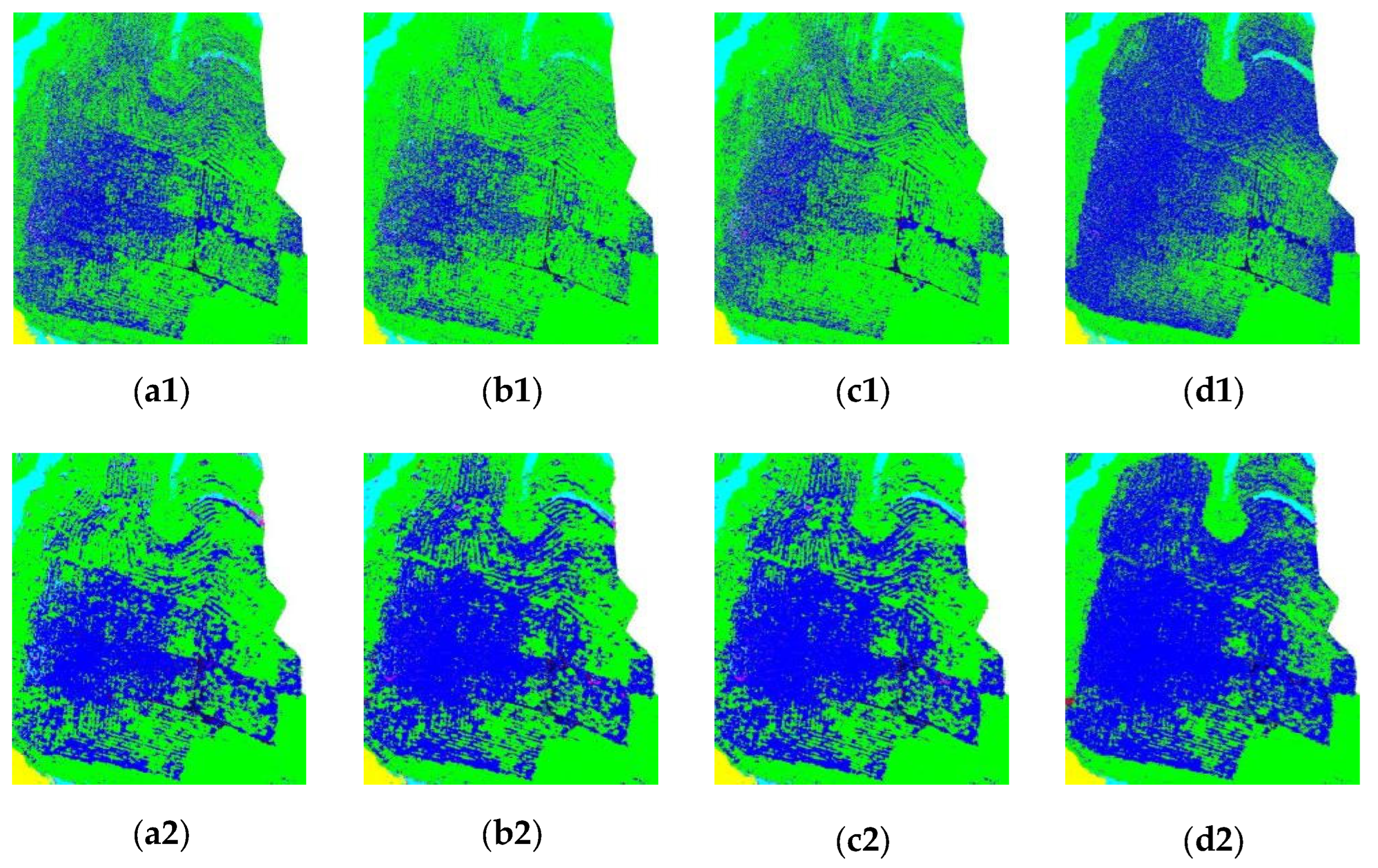
4.2. Classification of Solely LiDAR and the Combined LiDAR-SIF Data with One-Step Approach

Figure 6 presents the results of land-cover classification solely using LiDAR data. The classification was performed using a (a) decision tree classifier, (b) LightGBM classifier, (c) XGBoost classifier, and (d) random forest classifier. In these figures, different colors represent distinct land-cover types, and the legend indicates the corresponding colors and categories. The classification accuracy using the decision tree classifier is 76.07%, while the LightGBM classifier achieves 76.35%, the XGBoost classifier attains 76.36%, and the random forest classifier scores the highest at 83.31%.

Figure 7 depicts the results of the land-cover classification using the combined LiDAR and SIF data through one-step approach. The color map used in these figures is consistent with the previous description, utilizing the following classifiers: (a) decision tree classifier, (b) LightGBM classifier, (c) XGBoost classifier, and (d) random forest classifier. After incorporating fluorescence into the classification process, the decision tree classifier achieved an accuracy of 80.78%, the LightGBM classifier reached 83.38%, the XGBoost classifier attained 83.59%, and the random forest classifier scored an accuracy of 90.37%, demonstrating the enhancement performance of the SIF information.

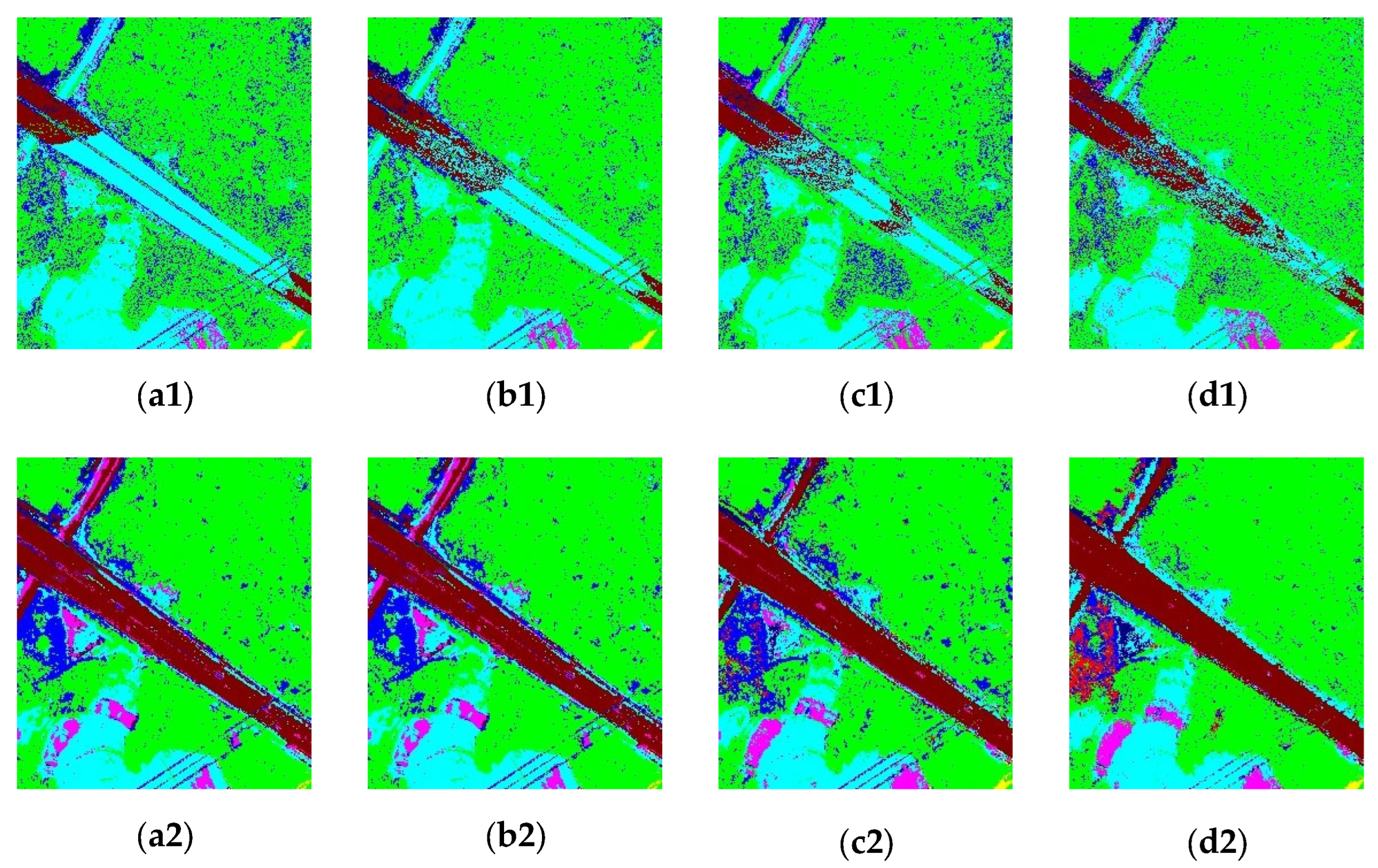
4.3. Classification of the Combined LiDAR and SIF Data with Multi-Stage Classification Strategy

Table 1. The accuracy of the first stage classification.

	Vegetation	Non-Vegetation	Overall Accuracy
Decision tree classifier	96.45%	84.77%	96.41%
LightGBM classifier	97.95%	79.04%	96.81%
XGBoost classifier	97.97%	78.70%	96.79%
Random forest classifier	98.92%	83.69%	97.71%

shows the accuracy of the first stage classification, with each classifier achieving an accuracy of over 96.45%, laying a good foundation for the subsequent classification.

Figure 8 showcases the results of land-cover classification using a multi-stage classification strategy combining LiDAR and SIF. The color map and classifiers utilized in these figures are consistent with the previous description. For the accuracy evaluation, the decision tree classifier achieved an overall classification accuracy of 83.52%, while the LightGBM classifier attained 86.25%. Meanwhile, the XGBoost classifier demonstrated an accuracy of 86.48% and the random forest classifier exhibited superior performance, scoring an impressive overall accuracy of 92.45%. In Figure 9, the bar charts show the classification performance of the various classifiers using LiDAR alone, fusing LiDAR and SIF through one-step approach, and combining LiDAR and SIF with multi-stage strategy.

Table 2. The overall accuracy of the land-cover classification of all strategies.

Data	LiDAR	LiDAR and Multi-Spectral Image		LiDAR and SIF
Method	One-Step Approach	One-Step Approach	Multi-Stage Strategy	One-Step Approach	Multi-Stage Strategy
Decision tree classifier	76.07%	76.89%	80.53%	80.78%	83.52%
LightGBM classifier	76.36%	82.00%	82.49%	83.38%	86.25%
XGBoost classifier	76.36%	82.16%	82.69%	83.59%	86.48%
Random forest classifier	83.31%	88.91%	89.36%	90.37%	92.45%

shows the overall accuracy of land-cover classification for all strategies: LiDAR solely, LiDAR integrated SIF using one-step approach and multi-step strategy, LiDAR integrated multispectral image using one-step approach and multi-step strategy.

5. Discussion

5.1. Analysis of the SIF-Enhanced Classification Effectiveness Using LiDAR Data

The integration of SIF data with LiDAR offers a promising avenue for enhancing land-cover classification accuracy. Our analysis reveals that the joint LiDAR-SIF classification outperforms the standalone LiDAR classification across various classifiers (Table 2). The classifiers utilized, including decision tree, XGBoost, random forest, and LightGBM, consistently demonstrate superior classification results when incorporating SIF data. The effectiveness of the SIF-enhanced classification is evident in the accuracy improvement range, ranging from 4.71% to 7.23% when compared with the standalone LiDAR classification. This improvement, achieved with relatively low computational costs, underscores the potential of SIF data in improving land-cover classification accuracy.

We further compare the results of LiDAR integrated SIF and integrated LiDAR and optical image feature classification in this experimental area. In Table 2, LiDAR integrated SIF presents advantages in accuracy. In different classifier methods, the accuracy of LiDAR integrated SIF is 1.39% to 3.89% higher than that of LiDAR and multispectral data. The result further illustrates the feasibility and advantages of SIF applied to the land-cover classification.

In most rural settings, the area covered by the vegetation regions is often significantly larger than that of the built-up areas, resulting in a relative scarcity of training samples for non-vegetation categories. This imbalance results in several challenges. First, some buildings can be confused with tall trees due to their similar heights. Second, sparsely distributed small-area building regions are often misclassified as the most proximal large-area vegetation category. The strategy of combining LiDAR and SIF data effectively addresses these challenges. This strategy leverages the complementary strengths of both data sources to enhance the separability of different land-cover types, particularly in the areas where vegetation and built-up regions coexist. The resulting classification maps shown in Figure 7 exhibit clearer boundaries and more accurate representations of land-cover types than in Figure 6, with optimized distinctions between water bodies, buildings, and vegetation.

Visual inspection reveals that the classification results solely derived from the LiDAR dataset (first line in Figure 10) exhibit blurred boundaries and notable misclassifications in large and scattered regions. In the second line of the presented classification maps, arbor forest B, which is represented by blue, vividly demonstrates the optimization effect achieved through the introduction of SIF data. In the comparison of the different classification methods, namely, decision tree, XGBoost, random forest, and LightGBM—we observe a significant increase in the area of correct classification, along with a marked improvement in the clarity of feature boundaries.

The surfaced road, which is depicted in brown located within vast vegetation areas exhibited fragmented and erroneous classification when relying solely on LiDAR data (Figure 11). The road was typically mistakenly categorized as grasslands for similar geometric features and heights. With the integration of SIF data for classification, significant improvements were made in error correction, resulting in more clearly defined and complete boundaries for surfaced road across various classifiers.

5.2. Exploration of the Classification Results through Fusion of LiDAR and SIF Data Utilizing Multi-Stage Classification Strategy

After verifying the effectiveness of SIF-enhanced LiDAR land-cover classification, multi-stage classification strategy was further adopted to deeply explore the potential of fluorescence information in land-cover classification. The implementation of multi-stage classification strategy combining LiDAR and SIF achieved better results compared to solely LiDAR classification or simply combining LiDAR and SIF, fully verifying the effectiveness and feasibility of the multi-stage strategy (Table 2). The joint LiDAR and SIF classification method adopting multi-stage classification strategy has an overall classification accuracy between 83.51% and 92.45%, which has an accuracy improvement range of 6.65% to 9.12% compared with standalone LiDAR classification, showing significant advantages in accuracy among various classification methods such as decision tree, XGBoost, random forest, and LightGBM.

The experimental results indicate that the classification effect achieved using random forest was optimal. This outcome can be attributed to several factors. First, the training samples in the experimental area were not uniformly distributed, and random forest has a relative advantage in adjusting weights, enabling it to fully utilize the available features. Second, the parameter tuning for random forest is relatively straightforward, facilitating efficient usage and optimization. Additionally, random forest is a powerful classification method that exhibits robustness to noise, which contributed to its excellent performance in this experiment.

The incorporation of SIF information significantly improves the recognition capability of LiDAR to identify various categories, as illustrated in the detailed classification accuracy bar chart in Figure 9. Furthermore, the implementation of the multi-stage classification strategy resulted in another stepwise increase in classification accuracy, with only a few cases showing inconsistency. This trend remains consistent across all classifiers. The bar chart indicates that the method of employing multi-stage strategy yields a higher accuracy in various categories than combining LiDAR and SIF data through one-step approach. This improvement is particularly noticeable in non-vegetation categories, as the first-stage classification greatly rectified the misclassifications of non-vegetation categories as vegetation categories.

The multi-step classification strategy effectively leverages the inherent sensitivity of SIF to vegetation characteristics. As illustrated in Table 2, LiDAR integrated SIF demonstrates a precision advantage over LiDAR integrated multi-spectral image when employing the multi-step classification strategy. Our analysis reveals that LiDAR integrated multi-spectral image, when utilized within a multi-step classification framework, yields negligible improvement over one-step classification, with a marginal increase of approximately 0.50%. In stark contrast, the adoption of the multi-step classification strategy consistently enhances accuracy by at least 2.50% for LiDAR integrated SIF. This disparity stems from the fact that SIF, in comparison to traditional optical imagery, exhibits a closer correlation with the physiological attributes of vegetation, thereby offering superior capabilities to distinguish.

In the multi-step classification process, traditional optical imagery initially proves less adept at distinguishing between vegetation and non-vegetation, leading to misclassified pixels that subsequently interfere with classifier decisions during further classification stages, thus impacting overall accuracy. Consequently, the final outcome and accuracy of one-step classification remain largely unchanged. Conversely, owing to the strong correlation between SIF and vegetation physiology, preliminary classification achieves high precision. Therefore, the integration of a multi-step classification strategy with SIF data proves highly effective.

To gain a clearer understanding of the role of SIF information in the classification process, the confusion matrix results of the random forest method was utilized to analyze the effect of SIF as an example. By calculating the confusion matrix, the user’s accuracy for each class is recorded in

Table 3. Matrix of user’s accuracy for the standalone LiDAR land-cover classification using random forest classifier.

	Arbor Forest A	Arbor Forest B	Bamboo Forest	Grassland	Farmland	Water	Bareland	Imprevious land	Surfaced Road	Unsurfaced Road	Residence	Other Building
Arbor forest A	58.69%	36.88%	0.02%	1.82%	0.56%	0.01%	0.98%	0.56%	0.45%	0.00%	0.01%	0.03%
Arbor forest B	3.54%	93.85%	0.01%	1.42%	0.32%	0.15%	0.38%	0.12%	0.19%	0.00%	0.00%	0.01%
Bamboo forest	18.74%	68.70%	4.29%	5.29%	1.04%	0.31%	0.91%	0.26%	0.41%	0.00%	0.03%	0.02%
Grassland	4.50%	13.75%	0.02%	77.36%	1.60%	0.17%	0.67%	0.91%	0.95%	0.00%	0.01%	0.05%
Farmland	7.50%	22.52%	0.03%	25.22%	40.58%	0.13%	2.39%	0.53%	1.08%	0.00%	0.01%	0.02%
Water	2.06%	21.44%	0.03%	10.58%	1.20%	63.84%	0.38%	0.07%	0.38%	0.00%	0.00%	0.00%
Bareland	7.18%	16.34%	0.02%	1.56%	0.95%	0.09%	65.72%	5.78%	2.07%	0.00%	0.04%	0.26%
Imprevious land	5.68%	6.66%	0.02%	0.79%	0.16%	0.01%	16.80%	67.68%	1.77%	0.00%	0.05%	0.38%
Surfaced road	9.52%	29.13%	0.03%	8.32%	2.07%	0.03%	6.06%	4.48%	40.24%	0.00%	0.06%	0.05%
Unsurfaced road	23.85%	50.09%	0.08%	6.21%	2.71%	0.05%	8.24%	2.77%	3.70%	1.96%	0.21%	0.13%
Residence	32.53%	25.83%	0.14%	1.80%	1.51%	0.01%	10.85%	6.90%	7.46%	0.01%	12.74%	0.21%
Other building	15.83%	32.65%	0.07%	3.15%	1.76%	0.43%	10.38%	6.36%	1.17%	0.01%	0.13%	28.06%

,

Table 4. Matrix of user’s accuracy for the joint LiDAR-SIF land-cover classification using random forest classifier.

	Arbor Forest A	Arbor Forest B	Bamboo Forest	Grassland	Farmland	Water	Bareland	Imprevious Land	Surfaced Road	Unsurfaced Road	Residence	Other Building
Arbor forest A	56.48%	38.96%	0.58%	1.77%	0.63%	0.00%	0.66%	0.10%	0.73%	0.01%	0.07%	0.01%
Arbor forest B	6.85%	90.16%	0.37%	1.40%	0.40%	0.10%	0.37%	0.07%	0.23%	0.00%	0.03%	0.02%
Bamboo forest	30.38%	45.97%	14.12%	5.06%	2.12%	0.17%	0.91%	0.09%	0.75%	0.01%	0.38%	0.02%
Grassland	6.06%	10.16%	0.26%	78.92%	2.02%	0.19%	0.67%	0.80%	0.80%	0.00%	0.04%	0.08%
Farmland	7.68%	11.66%	0.47%	15.59%	62.39%	0.12%	0.79%	0.38%	0.74%	0.01%	0.14%	0.02%
Water	1.91%	14.56%	0.22%	5.78%	1.69%	75.23%	0.07%	0.00%	0.54%	0.00%	0.00%	0.00%
Bareland	5.80%	8.31%	0.37%	1.51%	1.06%	0.08%	76.50%	3.69%	2.23%	0.01%	0.21%	0.22%
Imprevious land	2.87%	2.97%	0.04%	0.55%	0.57%	0.00%	13.57%	76.15%	1.90%	0.01%	0.73%	0.64%
Surfaced road	7.42%	16.07%	0.23%	2.63%	1.74%	0.16%	6.45%	1.80%	63.23%	0.02%	0.19%	0.07%
Unsurfaced road	34.64%	28.60%	1.06%	3.95%	5.46%	0.00%	11.90%	1.55%	6.40%	3.86%	2.13%	0.45%
Residence	22.67%	10.54%	0.66%	0.97%	3.46%	0.00%	7.08%	5.06%	17.04%	0.03%	32.29%	0.20%
Other building	12.80%	17.09%	0.32%	2.14%	2.59%	0.03%	12.38%	9.60%	3.97%	0.16%	1.41%	37.50%

and

Table 5. Matrix of user’s accuracy for the joint LiDAR-SIF classification with multi-stage classification strategy using random forest classifier.

	Arbor Forest A	Arbor Forest B	Bamboo Forest	Grassland	Farmland	Water	Bareland	Imprevious Land	Surfaced Road	Unsurfaced Road	Residence	Other Building
Arbor forest A	75.77%	22.30%	0.28%	1.16%	0.32%	0.00%	0.07%	0.00%	0.09%	0.00%	0.00%	0.00%
Arbor forest B	3.24%	95.46%	0.15%	0.79%	0.19%	0.06%	0.06%	0.00%	0.04%	0.00%	0.00%	0.00%
Bamboo forest	23.66%	33.54%	37.57%	3.70%	1.16%	0.11%	0.08%	0.00%	0.17%	0.00%	0.01%	0.00%
Grassland	5.01%	6.76%	0.16%	86.97%	0.85%	0.11%	0.03%	0.01%	0.10%	0.00%	0.00%	0.00%
Farmland	6.58%	10.15%	0.19%	10.88%	71.84%	0.08%	0.08%	0.01%	0.18%	0.00%	0.00%	0.00%
Water	1.90%	10.54%	0.15%	4.05%	0.90%	82.35%	0.04%	0.00%	0.06%	0.00%	0.00%	0.00%
Bareland	0.16%	0.24%	0.01%	0.10%	0.09%	0.01%	95.65%	2.20%	1.09%	0.01%	0.21%	0.22%
Imprevious land	0.32%	0.29%	0.02%	0.09%	0.05%	0.00%	7.52%	89.74%	1.00%	0.01%	0.50%	0.45%
Surfaced road	0.63%	0.65%	0.01%	0.40%	0.26%	0.01%	4.04%	1.31%	92.43%	0.02%	0.18%	0.07%
Unsurfaced road	4.11%	4.02%	0.49%	1.18%	2.72%	0.00%	18.13%	2.89%	6.67%	52.64%	6.18%	0.98%
Residence	1.50%	1.45%	0.34%	0.16%	0.39%	0.00%	5.79%	2.82%	6.64%	0.11%	80.40%	0.38%
Other building	0.59%	1.09%	0.06%	0.38%	0.41%	0.04%	10.05%	7.75%	2.65%	0.13%	1.60%	75.26%

.

Given that the non-vegetation types are mostly artificially constructed buildings and roads, the spatial distribution of non-vegetation is relatively fragmented and small compared with natural vegetation. Classification confusion often occurs at the boundaries, especially between buildings and arbor forest with similar heights. In Table 4, although the introduction of SIF has improved the accuracy of classification, many pixels of various non-vegetation categories are still misplaced and classified into arbor forest A and arbor forest B. Taking residence as an example, when only using LiDAR for classification, 25.83% of it was mistakenly classified as arbor forest B. After introducing SIF, this value decreased to 10.54%. What is more, only 1.45% of residences were misplaced as arbor forest B after using multi-stage classification strategy, which achieved a very good optimization.

The geometric features of vegetation categories are similar among different species with similar heights and distributions. This situation poses a challenge for further classification, and the introduction of SIF helps in providing additional auxiliary information. For example, farmland and grassland exhibit similar geometric and texture features, resulting in a significant amount of confusion and misclassification. The result of the comparison of Table 3 and Table 5 indicated that the introduction of SIF spectral features could significantly reduce the confusion between farmland and grassland. The percentage of area in farmland mistakenly classified as grassland reduced from 25.22% to 15.59% by fusing SIF data through one-step approach, and reached 10.88% after utilizing multi-stage strategy, with a decrease of approximately 15%. SIF significantly mitigated the major misclassification between vegetation categories.

For non-vegetation categories, analysis of the confusion matrix from the LiDAR land-cover classification in the experimental area reveals that the ratio of buildings mistakenly classified as vegetation type such as arbor forests B, is much higher than the misclassification rate within fine non-vegetation categories. For example, the proportion of surfaced road misclassified into different non-vegetation categories ranged from 0 to 6.06%, while 29.13% of it have been incorrectly classified as arbor forest B and 9.52% as arbor forest A (shown in Table 3). After the first stage of classification where vegetation and non-vegetation were primarily classified, the surfaced road area that was misclassified as arbor forest B greatly declined to 0.65%, and the proportion misclassified as arbor forest A decreased by 0.63% as shown in Table 5, resulting in a significant improvement in the final classification accuracy of this category. The decrease in the values of nondiagonal elements in the confusion matrix proved that the initial classification using SIF effectively separates buildings from vegetation and greatly improves the situation where building types are incorrectly classified as vegetation.

In summary, the integration of SIF information, which is sensitive to photosynthetic activity, provides additional discriminatory power for distinguishing between vegetated and non-vegetated areas. The multi-stage classification step, which focuses on finer categories within each broad class, leverages the detailed structural information captured by LiDAR data and takes full advantage of the sensitivity to vegetation of SIF data. This combined approach allows for a more comprehensive and accurate representation of land-cover types, resulting in improved classification results.

5.3. Limitations and Expectations for the Current Research

In the context of SIF-optimized LiDAR land-cover classification, we hypothesized that the physiological information contained in SIF would enhance the classification of vegetation categories. However, contrary to our expectations, the optimization effect on non-vegetation categories was more significant than that on vegetation categories, regardless of whether a direct feature combination or a multi-stage classification strategy was used. This observation may be attributed to the fact that the SIF differences between vegetation and non-vegetation are more pronounced than those within fine-grained vegetation categories, resulting in relatively subtle optimization effects for vegetation categories.

During the experiment, we also encountered challenges in classifying certain categories, such as bamboo forests. Using LiDAR data alone was not sufficient for the successful classification. Although combining LiDAR information provided some improvement, it was still not effective in distinguishing bamboo forests. This situation underscores the difficulty posed by the scarcity of training samples for these categories and highlights the limitations of SIF information in distinguishing some fine-grained land-cover types.

Overall, although the integration of SIF and LiDAR data generally results in better land-cover classification performance compared with using single-band LiDAR alone, the effectiveness of the combined approach for certain categories is limited. Furthermore, the potential of SIF in enhancing the classification of vegetation categories has yet to be fully exploited. The optimization effect for the broader category of vegetation did not meet our initial expectations, indicating that further research is needed to address this issue. Future studies could explore more advanced feature extraction and classification techniques that can better capture and utilize the vegetation-related information contained in SIF data.

6. Conclusions

This study aimed to delve into and validate the potential application value of SIF in land-cover classification. We proposed a strategy of multi-stage classification using combined LiDAR and SIF information, along with a SIF spectral index that is conducive to classification. We achieved relatively excellent classification results with low computational costs, by incorporating SIF data with low-dimensional LiDAR features, achieving a maximum accuracy of 92.45%. This result validates the feasibility of applying SIF data to land-cover classification and enhancing the classification effectiveness of LiDAR data. Our results demonstrate that the integration of SIF and LiDAR data can lead to significant improvements in the accuracy of land-cover classification, especially for certain categories where LiDAR alone may not be sufficient. In conclusion, this study provides a foundation for future research on the application of SIF in land-cover classification, presenting new avenues for enhancing the accuracy and efficiency of remote-sensing-based land-cover mapping.

References

1. Pan, S.; Guan, H.; Chen, Y.; Yu, Y.; Nunes Gonçalves, W.; Marcato Junior, J.; Li, J. Land-Cover Classification of Multispectral LiDAR Data Using CNN with Optimized Hyper-Parameters. ISPRS J. Photogramm. Remote Sens. 2020, 166, 241–254. [Google Scholar] [CrossRef]
2. Antonarakis, A.S.; Richards, K.S.; Brasington, J. Object-Based Land Cover Classification Using Airborne LiDAR. Remote Sens. Environ. 2008, 112, 2988–2998. [Google Scholar] [CrossRef]
3. Object-Based Land Cover Classification Using High-Posting-Density LiDAR Data. GISci. Remote Sens. 2008, 45, 209–228. Available online: https://www.tandfonline.com/doi/abs/10.2747/1548-1603.45.2.209 (accessed on 18 March 2024). [CrossRef]
4. Yan, W.Y.; Shaker, A.; El-Ashmawy, N. Urban Land Cover Classification Using Airborne LiDAR Data: A Review. Remote Sens. Environ. 2015, 158, 295–310. [Google Scholar] [CrossRef]
5. Sebastian, G.; Vattem, T.; Lukic, L.; Bürgy, C.; Schumann, T. RangeWeatherNet for LiDAR-Only Weather and Road Condition Classification. In Proceedings of the 2021 IEEE Intelligent Vehicles Symposium (IV), Nagoya, Japan, 11–17 July 2021; pp. 777–784. [Google Scholar]
6. Swatantran, A.; Tang, H.; Barrett, T.; DeCola, P.; Dubayah, R. Rapid, High-Resolution Forest Structure and Terrain Mapping over Large Areas Using Single Photon Lidar. Sci. Rep. 2016, 6, 28277. [Google Scholar] [CrossRef]
7. Bijelic, M.; Gruber, T.; Mannan, F.; Kraus, F.; Ritter, W.; Dietmayer, K.; Heide, F. Seeing through Fog without Seeing Fog: Deep Multimodal Sensor Fusion in Unseen Adverse Weather. In Proceedings of the 2020 IEEE/CVF Conference on Computer Vision and Pattern Recognition (CVPR), Seattle, WA, USA, 13–19 June 2020; pp. 11682–11692. [Google Scholar]
8. Wallace, A.M.; Halimi, A.; Buller, G.S. Full Waveform LiDAR for Adverse Weather Conditions. IEEE Trans. Veh. Technol. 2020, 69, 7064–7077. [Google Scholar] [CrossRef]
9. Song, J.-H.; Han, S.-H.; Yu, K.Y.; Kim, Y.-I. Assessing the Possibility of Land-Cover Classification Using Lidar Intensity Data. Int. Arch. Photogramm. Remote Sens. Spat. Inf. Sci. 2002, 34, 259–262. [Google Scholar]
10. Zhou, W. An Object-Based Approach for Urban Land Cover Classification: Integrating LiDAR Height and Intensity Data. IEEE Geosci. Remote Sens. Lett. 2013, 10, 928–931. [Google Scholar] [CrossRef]
11. Rossini, M.; Nedbal, L.; Guanter, L.; Ač, A.; Alonso, L.; Burkart, A.; Cogliati, S.; Colombo, R.; Damm, A.; Drusch, M.; et al. Red and Far Red Sun-induced Chlorophyll Fluorescence as a Measure of Plant Photosynthesis. Geophys. Res. Lett. 2015, 42, 1632–1639. [Google Scholar] [CrossRef]
12. Jonard, F.; De Canniere, S.; Brüggemann, N.; Gentine, P.; Gianotti, D.S.; Lobet, G.; Miralles, D.G.; Montzka, C.; Pagán, B.R.; Rascher, U. Value of Sun-Induced Chlorophyll Fluorescence for Quantifying Hydrological States and Fluxes: Current Status and Challenges. Agric. For. Meteorol. 2020, 291, 108088. [Google Scholar] [CrossRef]
13. Aasen, H.; Van Wittenberghe, S.; Sabater Medina, N.; Damm, A.; Goulas, Y.; Wieneke, S.; Hueni, A.; Malenovskỳ, Z.; Alonso, L.; Pacheco-Labrador, J. Sun-Induced Chlorophyll Fluorescence II: Review of Passive Measurement Setups, Protocols, and Their Application at the Leaf to Canopy Level. Remote Sens. 2019, 11, 927. [Google Scholar] [CrossRef]
14. Sun, Y.; Frankenberg, C.; Wood, J.D.; Schimel, D.S.; Jung, M.; Guanter, L.; Drewry, D.T.; Verma, M.; Porcar-Castell, A.; Griffis, T.J.; et al. OCO-2 Advances Photosynthesis Observation from Space via Solar-Induced Chlorophyll Fluorescence. Science 2017, 358, eaam5747. [Google Scholar] [CrossRef]
15. Daumard, F.; Goulas, Y.; Champagne, S.; Fournier, A.; Ounis, A.; Olioso, A.; Moya, I. Continuous Monitoring of Canopy Level Sun-Induced Chlorophyll Fluorescence during the Growth of a Sorghum Field. IEEE Trans. Geosci. Remote Sens. 2012, 50, 4292–4300. [Google Scholar] [CrossRef]
16. Pinto, F.; Celesti, M.; Acebron, K.; Alberti, G.; Cogliati, S.; Colombo, R.; Juszczak, R.; Matsubara, S.; Miglietta, F.; Palombo, A.; et al. Dynamics of Sun-induced Chlorophyll Fluorescence and Reflectance to Detect Stress-induced Variations in Canopy Photosynthesis. Plant Cell Environ. 2020, 43, 1637–1654. [Google Scholar] [CrossRef] [PubMed]
17. Liu, L.; Guan, L.; Liu, X. Directly Estimating Diurnal Changes in GPP for C3 and C4 Crops Using Far-Red Sun-Induced Chlorophyll Fluorescence. Agric. For. Meteorol. 2017, 232, 1–9. [Google Scholar] [CrossRef]
18. Chen, S.; Huang, Y.; Wang, G. Detecting Drought-Induced GPP Spatiotemporal Variabilities with Sun-Induced Chlorophyll Fluorescence during the 2009/2010 Droughts in China. Ecol. Indic. 2021, 121, 107092. [Google Scholar] [CrossRef]
19. Daumard, F.; Champagne, S.; Fournier, A.; Goulas, Y.; Ounis, A.; Hanocq, J.-F.; Moya, I. A Field Platform for Continuous Measurement of Canopy Fluorescence. IEEE Trans. Geosci. Remote Sens. 2010, 48, 3358–3368. [Google Scholar] [CrossRef]
20. Yang, P.; van der Tol, C.; Verhoef, W.; Damm, A.; Schickling, A.; Kraska, T.; Muller, O.; Rascher, U. Using Reflectance to Explain Vegetation Biochemical and Structural Effects on Sun-Induced Chlorophyll Fluorescence. Remote Sens. Environ. 2019, 231, 110996. [Google Scholar] [CrossRef]
21. Watanachaturaporn, P.; Arora, M.K.; Varshney, P.K. Multisource Classification Using Support Vector Machines. Photogramm. Eng. Remote Sens. 2008, 74, 239–246. [Google Scholar] [CrossRef]
22. Pedergnana, M.; Marpu, P.R.; Dalla Mura, M.; Benediktsson, J.A.; Bruzzone, L. Classification of Remote Sensing Optical and LiDAR Data Using Extended Attribute Profiles. IEEE J. Sel. Top. Signal Process. 2012, 6, 856–865. [Google Scholar] [CrossRef]
23. Xu, L.; Shi, S.; Gong, W.; Chen, B.; Sun, J.; Xu, Q.; Bi, S. Mapping 3D Plant Chlorophyll Distribution from Hyperspectral LiDAR by a Leaf-Canopyradiative Transfer Model. Int. J. Appl. Earth Obs. Geoinf. 2024, 127, 103649. [Google Scholar] [CrossRef]
24. Xu, L.; Shi, S.; Gong, W.; Shi, Z.; Qu, F.; Tang, X.; Chen, B.; Sun, J. Improving Leaf Chlorophyll Content Estimation through Constrained PROSAIL Model from Airborne Hyperspectral and LiDAR Data. Int. J. Appl. Earth Obs. Geoinf. 2022, 115, 103128. [Google Scholar] [CrossRef]
25. Teo, T.-A.; Huang, C.-H. Object-Based Land Cover Classification Using Airborne Lidar and Different Spectral Images. TAO Terr. Atmos. Ocean. Sci. 2016, 27, 491. [Google Scholar] [CrossRef]
26. Lu, D.; Hetrick, S.; Moran, E. Land Cover Classification in a Complex Urban-Rural Landscape with QuickBird Imagery. Photogramm. Eng. Remote Sens. 2010, 76, 1159–1168. [Google Scholar] [CrossRef] [PubMed]
27. Buján, S.; González-Ferreiro, E.; Reyes-Bueno, F.; Barreiro-Fernández, L.; Crecente, R.; Miranda, D. Land Use Classification from Lidar Data and Ortho-Images in a Rural Area. Photogramm. Rec. 2012, 27, 401–422. [Google Scholar] [CrossRef]
28. Brown, D.G.; Johnson, K.M.; Loveland, T.R.; Theobald, D.M. Rural land-use trends in the conterminous united states, 1950–2000. Ecol. Appl. 2005, 15, 1851–1863. [Google Scholar] [CrossRef]
29. Rogan, J.; Chen, D. Remote Sensing Technology for Mapping and Monitoring Land-Cover and Land-Use Change. Prog. Plan. 2004, 61, 301–325. [Google Scholar] [CrossRef]
30. Tilahun, A.; Teferie, B. Accuracy Assessment of Land Use Land Cover Classification Using Google Earth. Am. J. Environ. Prot. 2015, 4, 193–198. [Google Scholar] [CrossRef]
31. Jansen, L.J.; Di Gregorio, A. Land-Use Data Collection Using the “Land Cover Classification System”: Results from a Case Study in Kenya. Land. Use Policy 2003, 20, 131–148. [Google Scholar] [CrossRef]
32. Vargo, J.; Habeeb, D.; Stone, B., Jr. The Importance of Land Cover Change across Urban–Rural Typologies for Climate Modeling. J. Environ. Manag. 2013, 114, 243–252. [Google Scholar] [CrossRef]
33. RIEGL—Produktdetail. Available online: http://www.riegl.com/nc/products/airborne-scanning/produktdetail/product/scanner/69/ (accessed on 19 March 2024).
34. Miko Scientists Confirm Specim’s AisaIBIS Reliably Measures Plant Stress. Specim 2015. Available online: https://www.specim.com/scientists-confirm-specims-aisaibis-reliably-measures-plant-stress/ (accessed on 19 March 2024).
35. Jakubowski, M.K.; Li, W.; Guo, Q.; Kelly, M. Delineating Individual Trees from LiDAR Data: A Comparison of Vector-and Raster-Based Segmentation Approaches. Remote Sens. 2013, 5, 4163–4186. [Google Scholar] [CrossRef]
36. Budei, B.C.; St-Onge, B. Variability of Multispectral Lidar 3D and Intensity Features with Individual Tree Height and Its Influence on Needleleaf Tree Species Identification. Can. J. Remote Sens. 2018, 44, 263–286. [Google Scholar] [CrossRef]
37. Liu, X.; Zhang, Z.; Peterson, J.; Chandra, S. The Effect of LiDAR Data Density on DEM Accuracy. In Proceedings of the 17th International Congress on Modelling and Simulation (MODSIM07), Canberra, Australia, 10–13 December 2007; Modelling and Simulation Society of Australia and New Zealand: Canberra, Australia, 2007. [Google Scholar]
38. Chehata, N.; Guo, L.; Mallet, C. Airborne Lidar Feature Selection for Urban Classification Using Random Forests. In Proceedings of the Laserscanning, Paris, France, 1–2 September 2009. [Google Scholar]
39. Ramadhani, A.N.R. An Analysis of the Three-Dimensional Modelling Using LiDAR Data and Unmanned Aerial Vehicle (UAV) (Case Study: Institut Teknologi Sepuluh Nopember, Sukolilo Campus). In IOP Conference Series: Earth and Environmental Science; IOP Publishing: Bristol, UK, 2023; Volume 1127, p. 012010. [Google Scholar]
40. Brodu, N.; Lague, D. 3D Terrestrial Lidar Data Classification of Complex Natural Scenes Using a Multi-Scale Dimensionality Criterion: Applications in Geomorphology. ISPRS J. Photogramm. Remote Sens. 2012, 68, 121–134. [Google Scholar] [CrossRef]
41. Automatic Detection and Mapping of Highway Guardrails from Mobile Lidar Point Clouds|IEEE Conference Publication|IEEE Xplore. Available online: https://ieeexplore.ieee.org/abstract/document/9553055 (accessed on 19 March 2024).
42. Daumard, F.; Goulas, Y.; Ounis, A.; Pedrós, R.; Moya, I. Measurement and Correction of Atmospheric Effects at Different Altitudes for Remote Sensing of Sun-Induced Fluorescence in Oxygen Absorption Bands. IEEE Trans. Geosci. Remote Sens. 2015, 53, 5180–5196. [Google Scholar] [CrossRef]
43. Damm, A.; Guanter, L.; Laurent, V.C.; Schaepman, M.E.; Schickling, A.; Rascher, U. FLD-Based Retrieval of Sun-Induced Chlorophyll Fluorescence from Medium Spectral Resolution Airborne Spectroscopy Data. Remote Sens. Environ. 2014, 147, 256–266. [Google Scholar] [CrossRef]
44. Plascyk, J.A.; Gabriel, F.C. The Fraunhofer Line Discriminator MKII-an Airborne Instrument for Precise and Standardized Ecological Luminescence Measurement. IEEE Trans. Instrum. Meas. 1975, 24, 306–313. [Google Scholar] [CrossRef]
45. Plascyk, J.A. The MK II Fraunhofer Line Discriminator (FLD-II) for Airborne and Orbital Remote Sensing of Solar-Stimulated Luminescence. Opt. Eng. 1975, 14, 339. [Google Scholar] [CrossRef]
46. Zhang, Y.; Guanter, L.; Berry, J.A.; Joiner, J.; Van Der Tol, C.; Huete, A.; Gitelson, A.; Voigt, M.; Köhler, P. Estimation of Vegetation Photosynthetic Capacity from Space-based Measurements of Chlorophyll Fluorescence for Terrestrial Biosphere Models. Glob. Chang. Biol. 2014, 20, 3727–3742. [Google Scholar] [CrossRef]
47. Yang, H.; Yang, X.; Zhang, Y.; Heskel, M.A.; Lu, X.; Munger, J.W.; Sun, S.; Tang, J. Chlorophyll Fluorescence Tracks Seasonal Variations of Photosynthesis from Leaf to Canopy in a Temperate Forest. Glob. Chang. Biol. 2017, 23, 2874–2886. [Google Scholar] [CrossRef]
48. Guanter, L.; Zhang, Y.; Jung, M.; Joiner, J.; Voigt, M.; Berry, J.A.; Frankenberg, C.; Huete, A.R.; Zarco-Tejada, P.; Lee, J.-E.; et al. Global and Time-Resolved Monitoring of Crop Photosynthesis with Chlorophyll Fluorescence. Proc. Natl. Acad. Sci. USA 2014, 111, E1327–E1333. [Google Scholar] [CrossRef]
49. Song, Y.-Y.; Ying, L.U. Decision Tree Methods: Applications for Classification and Prediction. Shanghai Arch. Psychiatry 2015, 27, 130. [Google Scholar] [PubMed]
50. Charbuty, B.; Abdulazeez, A. Classification Based on Decision Tree Algorithm for Machine Learning. J. Appl. Sci. Technol. Trends 2021, 2, 20–28. [Google Scholar] [CrossRef]
51. Myles, A.J.; Feudale, R.N.; Liu, Y.; Woody, N.A.; Brown, S.D. An Introduction to Decision Tree Modeling. J. Chemom. 2004, 18, 275–285. [Google Scholar] [CrossRef]
52. Breiman, L. Random Forests. Mach. Learn. 2001, 45, 5–32. [Google Scholar] [CrossRef]
53. Biau, G. Analysis of a Random Forests Model. J. Mach. Learn. Res. 2012, 13, 1063–1095. [Google Scholar]
54. Bui, Q.-T.; Chou, T.-Y.; Hoang, T.-V.; Fang, Y.-M.; Mu, C.-Y.; Huang, P.-H.; Pham, V.-D.; Nguyen, Q.-H.; Anh, D.T.N.; Pham, V.-M. Gradient Boosting Machine and Object-Based CNN for Land Cover Classification. Remote Sens. 2021, 13, 2709. [Google Scholar] [CrossRef]
55. McCarty, D.A.; Kim, H.W.; Lee, H.K. Evaluation of Light Gradient Boosted Machine Learning Technique in Large Scale Land Use and Land Cover Classification. Environments 2020, 7, 84. [Google Scholar] [CrossRef]
56. Ke, G.; Meng, Q.; Finley, T.; Wang, T.; Chen, W.; Ma, W.; Ye, Q.; Liu, T.-Y. Lightgbm: A Highly Efficient Gradient Boosting Decision Tree. Adv. Neural Inf. Process. Syst. 2017, 30, 1–9. [Google Scholar]
57. Torlay, L.; Perrone-Bertolotti, M.; Thomas, E.; Baciu, M. Machine Learning–XGBoost Analysis of Language Networks to Classify Patients with Epilepsy. Brain Inf. 2017, 4, 159–169. [Google Scholar] [CrossRef]
58. Ramraj, S.; Uzir, N.; Sunil, R.; Banerjee, S. Experimenting XGBoost Algorithm for Prediction and Classification of Different Datasets. Int. J. Control Theory Appl. 2016, 9, 651–662. [Google Scholar]
59. Chen, T.; Guestrin, C. XGBoost: A Scalable Tree Boosting System. In Proceedings of the 22nd ACM SIGKDD International Conference on Knowledge Discovery and Data Mining, San Francisco, CA, USA, 13 August 2016; ACM: New York, NY, USA, 2016; pp. 785–794. [Google Scholar]
Figure 1. The ground truth of the study area.
Remotesensing 16 01916 g001
Figure 2. The 3D display of the LiDAR dataset.
Remotesensing 16 01916 g002
Figure 3. The framework of the multi-stage classification fusing SIF and LiDAR for land-cover classification.
Remotesensing 16 01916 g003
Figure 4. Results of the point cloud feature extraction and rasterization: (a) height; (b) volume density; (c) verticality.
Remotesensing 16 01916 g004
Figure 5. Results of (a) SIF; (b) difference feature; (c) ratio feature.
Remotesensing 16 01916 g005
Figure 6. Classification results of the standalone LiDAR through different classifiers: (a) decision tree classifier; (b) LightGBM classifier; (c) XGBoost classifier; (d) random forest classifier.
Remotesensing 16 01916 g006
Figure 7. Classification results of fusing LiDAR and SIF with one-step approach through different classifiers: (a) decision tree classifier; (b) LightGBM classifier; (c) XGBoost classifier; (d) random forest classifier.
Remotesensing 16 01916 g007
Figure 8. Classification results of fusing LiDAR and SIF with multi-stage classification strategy through different classifiers: (a) decision tree classifier; (b) LightGBM classifiers; (c) XGBoost classifier; (d) random forest classifier.
Remotesensing 16 01916 g008
Figure 9. Comparison of the standalone LiDAR classification, fusing LiDAR and SIF with one-step approach, and fusing LiDAR and SIF with multi-stage classification strategy through different classifiers: (a) decision tree classifier; (b) LightGBM classifier; (c) XGBoost classifier; (d) random forest classifier.
Remotesensing 16 01916 g009
Figure 10. Classification result of the standalone LiDAR classification (first line) and fusing LiDAR and SIF with multi-stage classification (second line) through different classifiers: (a1) decision tree classifier; (b1) LightGBM classifier; (c1) XGBoost classifier; (d1) random forest classifier; (a2) decision tree classifier; (b2) LightGBM classifier; (c2) XGBoost classifier; (d2) random forest classifier.
Remotesensing 16 01916 g010
Figure 11. Classification result of the standalone LiDAR classification (first line) fusing LiDAR and SIF with multi-stage classification (second line) through different classifiers: (a1) decision tree classifier; (b1) LightGBM classifier; (c1) XGBoost classifier; (d1) random forest classifier; (a2) decision tree classifier; (b2) LightGBM classifier; (c2) XGBoost classifier; (d2) random forest classifier.
Remotesensing 16 01916 g011