Abstract
Urban planning has, in recent years, been significantly assisted by remote sensing data. The data and techniques that are used are very diverse and are available to government agencies as well as to private companies that are involved in planning urban and peri-urban areas. Synthetic aperture radar data are particularly important since they provide information on the geometric and electrical characteristics of ground objects and, at the same time, are unaffected by sunlight (day–night) and cloud cover. SAR data are usually combined with optical data (fusion) in order to increase the reliability of the terrain information. Most of the existing relative classification methods have been reviewed. New techniques that have been developed use decorrelation and interferometry to record changes on the Earth’s surface. Texture-based features, such as Markov random fields and co-occurrence matrices, are employed, among others, for terrain classification. Furthermore, target geometrical features are used for the same purpose. Among the innovative works presented in this manuscript are those dealing with tomographic SAR imaging for creating digital elevation models in urban areas. Finally, tomographic techniques and digital elevation models can render three-dimensional representations for a much better understanding of the urban region. The above-mentioned sources of information are integrated into geographic information systems, making them more intelligent. In this work, most of the previous techniques and methods are reviewed, and selected papers are highlighted in order for the reader-researcher to have a complete picture of the use of SAR in urban planning.
1. Introduction
In this introductory section, we delve into various facets related to the topic at hand, offering a comprehensive overview across multiple disciplines. We begin by shedding light on the features extracted from SAR (synthetic aperture radar) images specifically tailored for urban planning purposes. These features are meticulously chosen to capture the intricate details of urban environments, facilitating effective decision-making processes in urban development and management.
Moving forward, we explore the realm of classification and fusion algorithms utilized in SAR image analysis for delineating different categories within urban and suburban regions. These algorithms leverage advanced techniques to accurately identify and differentiate various urban features, such as buildings, roads, vegetation, and water bodies, among others. The synergistic fusion of information from multiple sources enhances the overall classification accuracy, enabling more precise urban mapping and analysis.
Furthermore, we delve into the significance of the decorrelation and interferometry properties inherent in SAR imagery. These properties play a pivotal role in detecting and classifying urban areas afflicted by natural disasters such as floods or earthquakes, as well as identifying structural damages in urban infrastructure. By leveraging the unique signatures captured by SAR, analysts can swiftly assess the extent of urban damage and formulate timely response strategies.
Lastly, we delve into the utilization of SAR data for the creation of digital elevation models (DEMs) and tomographic images in urban areas. DEM models derived from SAR data provide valuable insights into the topographic features of urban landscapes, aiding in urban planning, land management, and environmental monitoring. Additionally, SAR tomography techniques enable the reconstruction of three-dimensional images of urban structures, offering unprecedented levels of detail for various applications such as urban modeling and infrastructure assessment.
Overall, this introductory section serves as a comprehensive primer, laying the groundwork for further exploration into the intricate relationship between SAR imagery and urban environments.
1.1. Feature Extraction
Various types of features extracted from SAR data have been used so far for urban region segmentation, categorization, and change detection. In this paragraph, a collection of these types of features is presented. A Markov random field is employed in [1] to represent the urban road network as a feature when high-resolution SAR images are used. A Markov random field is a graphical model used to represent the probabilistic relationships between variables in a system. It is characterized by conditional independence properties, meaning that the probability of one variable depends only on the variables to which it is directly connected. Urban satellite SAR images are characterized by multiscale textural features, as introduced in [2]. Multiscale textural features refer to analyzing textures in an image or signal at multiple scales or levels of detail. This involves extracting information about the patterns, structures, and variations in texture across different spatial resolutions. It is commonly used in image processing, computer vision, and pattern recognition tasks to capture both local and global characteristics of textures. Texture-based discrimination is accurately achieved in the case of land cover classes based on the evaluation of the co-occurrence matrices and the parameters obtained as textural features. The authors in [3] retrieve information regarding the extension of the targets in range and azimuth based on the variation of the amplitude of the received radar signal. A new approach is proposed in [4] to determine the scattering properties of non-reflecting symmetric structures by means of circular polarization and correlation coefficients. In order to analyze the parameters necessary to estimate urban extent, a method is proposed in [5] and compared against reference global maps. A new method for automatically classifying urban regions into change and no change classes when using multitemporal spaceborne SAR data was based on a generalized version of the Kittler–Illingworth minimum-error thresholding algorithm [6]. In [7], the authors investigate a speckle denoising algorithm with nonlocal characteristics that associates local structures with global averaging when change detection is carried out in multitemporal SAR images. Urban heat island intensity is quantified in [8] based on SAR images and utilizing a specific local climate zone landscape classification system. The work in [9] aims at assessing the utility of spaceborne SAR images for enhancing global urban mapping. This is achieved through the implementation of a robust processing chain known as the KTH-Pavia Urban Extractor. Mutual information criteria employed by a filtering method were introduced in [10] in order to choose and classify the appropriate SAR decomposition parameters for classifying the site in Ottawa, Ontario. Mutual information measures the amount of information that one random variable contains about another random variable. It quantifies the degree of dependency between the variables. In [11], two methods were employed to evaluate urban area expansion at various scales. The first method utilized night-time images, while the second method relied on SAR imagery. SAR image co-registration was achieved by a fast and robust optical-flow estimation algorithm [12]. Urban land cover classification is carried out in [13] by comparing images from the Landsat OLI spaceborne sensor with the Landsat Thematic Mapper. The authors in [14] used rotated dihedral corner reflectors to form a decomposition method for PolSAR data over urban areas. Target decomposition methods are also employed in [15] for urban area detection using PolSAR images. Target decomposition methods refer to a class of techniques used in signal processing and data analysis to decompose a signal or dataset into constituent parts, often with the aim of isolating specific components of interest. Some common target decomposition methods include polarimetric decomposition techniques like Freeman–Durden decomposition and Cloude–Pottier decomposition, which are used to characterize and analyze polarimetric radar data. These methods help extract meaningful information about the scattering properties of targets or terrain surfaces from complex radar observations. The study discussed in [16] focuses on estimating future changes in land use/land cover due to rapid urbanization, which is known to significantly increase land surface temperatures in various regions around the world.
1.2. Classification Algorithms
Besides the features required for classifying urban regions using SAR images, the classification tools are equally important for this purpose. Classification approaches are revisited in this paragraph. In [17], the authors analyzed the potential of decision trees as a data mining procedure suitable for the analysis of remotely sensed data. Decision trees are a popular type of supervised machine learning algorithm used for both classification and regression tasks. They work by recursively partitioning the input space into smaller regions based on feature values, making decisions at each step based on the values of input features. The log-ratio change indicator thresholding is automated and made more effective in [18] for multitemporal single-polarization SAR images. In [19], a classification approach based on a deep belief network model for detailed urban mapping using PolSAR data is proposed. A deep belief network is a type of artificial neural network architecture composed of multiple layers of latent variables, typically arranged as a stack of restricted Boltzmann machines. It is an unsupervised learning model used for tasks like feature learning, dimensionality reduction, and generative modeling. The study conducted in [20] aims to assess the effectiveness of combining multispectral optical data and dual-polarization SAR for distinguishing urban impervious surfaces. An extended four-component model-based decomposition method is proposed in [21] for PolSAR data over urban areas by means of rotated dihedral corner reflectors. In [22] a new classification scheme is proposed that fully exploits SAR data for mapping urban impervious surfaces, avoiding methods that are restricted to optical images. In [23], how deep fully convolutional networks, operating as classifiers, can be designed to process multi-modal and multi-scale remote sensing data is studied. Deep fully convolutional networks are a type of neural network architecture designed for semantic segmentation tasks. A method employing deep convolutional neural networks is presented in [24] to overcome weaknesses in accuracy and efficiency for urban planning and land management. In [25], a highly novel joint deep learning framework, which combines a multilayer perceptron and a convolutional neural network, is recommended for land cover and land use classification. In [26], the authors review the major research papers regarding deep learning image classifiers and comment on their performance compared to support vector machine (SVM) classifiers. support vector machine classifiers are supervised learning models used for classification and regression tasks. SVMs are particularly effective for classification problems with two classes, but they can also be extended to handle multi-class classification. The study in [27] demonstrates that it is feasible to automatically and accurately carry out urban scene segmentation using high-resolution SAR data with the assistance of deep neural networks. The capability of visual and radar (SAR) data to accurately classify regions occupied by cities is tested in [28] by means of three supervised classification methods. Finally, since the fast changes in land cover/land use are a strong indication of global environmental change, it is important to monitor land cover/land use through maps [29].
1.3. Fusion of SAR and Multiband Images
Fusion techniques in various levels (raw data, features, and decisions) are very important to improve the information required for urban region characterization. Some recent fusion techniques that mainly combine visual and SAR images for urban planning are given in the following: A fusion method is proposed in [30], which carries out co-registration of SAR and optical images to provide an integrated map of an urban area. The method takes into consideration the fact that SAR point targets strongly characterize urban areas. In [31], InSAR and multi-spectral data are utilized for characterizing and monitoring urban areas, considering the underlying physics, geometry, and statistical behavior of the data. Change detection is faced in [32] by fusing multiple SAR images based on extracting and comparing pixel-based linear features. High-resolution interferometric SAR is shown in [33] to be an important basis for fusion with other remotely sensed data in urban analysis tasks. The work in [34] describes the capability of fusing optical and SAR images by means of an unsupervised procedure for operational rapid urban mapping. In the 2007 Data Fusion Contest organized by the IEEE Geoscience and Remote Sensing Data Fusion Technical Committee, SAR and optical data from satellite sensors were employed to extract land cover maps in and around urban areas. This was achieved by exploiting multitemporal and multisource coarse-resolution datasets [35]. The study presented in [36] had two main objectives. First, it aimed to compare the performances of various data fusion techniques with the goal of enhancing urban features. Second, it aimed to improve urban land cover classification by employing a refined Bayesian classification approach. The aim of the study in [37] was to combine Quickbird multispectral (MS) and RADARSAT SAR data to improve the mapping of the occupation and use of the land by city structures. The primary objective of [38] was to assess the integration of radar and optical data. This involved examining how different aspects of input data contributed to the performance of a random forest classifier in urban and peri-urban environments. The research in [39] focused on developing a novel procedure for utilizing coarse-resolution SAR images to determine both the extent of built-up areas and generate a map of the identified urban region. A novel and efficient approach was introduced in [40] to isolate robust city surfaces by combining visual and EM data for decision inference. In [41] the authors presented a convolutional neural network capable of identifying matching patches within complex urban scenes by means of fine resolution visual and SAR data. The research in [42] put forth a new methodology for assessing monthly changes in impervious surfaces by integrating time series data from Landsat and MODIS. The study in [43] primarily aims to determine the feasibility of mapping winter wheat during the growing season and assess whether incorporating SAR and optical data, both separately and combined, can enhance classification accuracy in urban agricultural areas. In [44], the key objectives are to explore the potential utility and combined benefits of using ESA Sentinel-1A C-band SAR data and Sentinel-2A MSI data for the classification and mapping of ecologically significant urban and peri-urban areas. Different integration levels between SAR and optical data are compared in [45] to provide a scientific reference for a variety of studies. A methodological framework is presented in [46] for combining optical and SAR data at a pixel-level fusion to improve urban land cover classification.
1.4. Decorrelation for Disaster Detection
Rapid changes in urban regions due to disasters can be recorded and analyzed by means of the correlation and coherence properties among the SAR pixels. Phase analysis, which is expressed by interferometry, is very closely related to the correlation and coherence properties of the pixels. Decorrelation is an attempt to decrease the autocorrelation within a single signal or the correlation between two signals. To achieve the minimum autocorrelation, the power spectrum of the signal is adjusted to resemble that of a white noise signal (whitening). On the other hand, coherence is a measure of the consistency and phase alignment between waves. In accordance with the above, interferometry is a technique that leverages the interference of superimposed waves to extract valuable information. It is used for precise measurements of microscopic displacements, monitoring refractive index changes, and characterizing surface irregularities. The above concepts have been applied to specific applications with SAR imagery, as described below.
The detection of damaged areas around Kobe city in Japan due to the 1995 earthquake was achieved by employing intensity correlation and coherence [47]. The correlation coefficients between pre-earthquake and post-earthquake data were evaluated as a normalized difference. Multi-temporal SAR images are utilized in [48] in an unsupervised change-detection method to detect new urban areas. This approach leverages both the coherence and intensity characteristics of SAR pixels. The study in [49] explores the hidden signatures in co-polarization coherence within the radar line of sight to investigate urban damage. A proposed damage index can differentiate between different levels of damage in urban patches. A high-resolution coherent change detection approach is introduced in [50] for identifying structural changes in urban areas by combining SAR imagery with GIS processing.
1.5. Interferometry for Change Detection in Urban Areas
The work in [51] demonstrates that individual buildings and infrastructure can be monitored for structural stress and seasonal deformation by means of the TerraSAR-X data because of the short revisiting time of the satellite (11 days). An optimal estimation method is presented in [52] for phase histories of distributed scatterers in urban areas. The method offers elevation and deformation accuracy comparable to persistent scatterer interferometry. The research presented in [53] explores the role of interferometric coherence in addition to intensity SAR data for mapping floods in both agricultural and urban environments. Interferometric data are effective in identifying areas with changes in water levels. The authors in [54] investigate the use of repeat-pass interferometric SAR for land cover classification. Their findings are that a greater loss of interferometric coherence exists as the time difference between two interferometric acquisitions increases. An unsupervised method for flood detection is presented in [55], which combines SAR intensity and interferometric coherence data.
1.6. Flood in Urban Areas
Flood dynamics in urban areas, as explained in [56], can be monitored using a unique dataset comprising eight space-borne SAR images, aerial photographs, and constrained mathematical models. In the study in [57], a complex urban area in Kuala Lumpur, Malaysia, was selected as a case study to simulate an extreme flooding event that occurred in 2003. Three different digital terrain models (DTMs) were structured and employed as input for a 2D urban flood model. The method presented in [58] had two main objectives: (a) to establish the connection among the water height and the flood range (SAR-derived flood images) for various river cross sections, and (b) to infer the location of embankments by identifying plateaus in these stage-extent plots. Airborne LiDAR data were employed to assess their estimation accuracy and reliability. A neuro-fuzzy flood mapping approach is presented in [59] by means of texture-enhanced single SAR images. The flood and non-flood categories are represented on a fuzzy inference system using Gaussian curves.
1.7. Digital Elevation Models and Tomographic Images of Urban Areas
Since the SAR images contain coherency and interferometric information, they are suitable for supporting the construction of DTMs and tomographic representations. One of the main advantages of high-resolution SAR images is that their information is independent of weather conditions. However, the inherent slant range geometry prohibits the whole ground information from being recorded, leaving large shadow areas. In [60], a review of TomoSAR techniques is provided, presenting relevant applications for urban areas and especially on scatterer 3D localization, selection of reliable scatterers, and precise regaining of the underlying surface. The circular trajectory of a SAR sensor around a specific region gives the capability of constructing a DEM of the region [61]. The work in [62] introduces a validation of SAR tomography regarding the analysis of a simple pixel-scatterer that consists of two different scattering mechanisms. The authors in [63] explain the achievable tomographic quality using TerraSAR-X spotlight data in an urban environment. They introduce a new Wiener-type regularization method for the singular-value decomposition technique, which likely enhances the quality of the tomographic reconstruction. The work in [64] proposes a complete processing chain capable of providing a simple 3-D reconstruction of buildings in urban scenes from a pair of high-resolution optical and SAR images. The essential role of SAR is highlighted [65] for layover separation in urban infrastructure monitoring. The paper likely provides geometric and statistical analysis to underscore the significance of SAR data in addressing layover issues in urban environments. The introduction of a new method for DEM extraction in urban areas using SAR imagery is presented in [66]. For the retrieval of the real 3-D localization and motion of scattering objects, advanced interferometric methods like persistent scatterer interferometry and SAR tomography are required, as discussed in [67]. The work in [68] aimed at a precise TomoSAR reconstruction by incorporating a priori knowledge, thus significantly reducing the required number of images for the estimation. The work in [69] focuses on the investigation of applying a stereogrammetry pipeline to very-high-resolution SAR-optical image pairs. A novel method for integrating SAR and optical image types is presented in [70]. The approach involves automatic feature matching and combined bundle adjustment between the two image types, aiming to optimize the geometry and texture of 3D models generated from aerial oblique imagery. The authors in [71] introduce a planarity-constrained multi-view depth map reconstruction method that begins with image segmentation and feature matching and involves iterative optimization under the constraints of planar geometry and smoothness. The capabilities of PolSAR tomography in investigating urban areas are analyzed in [72]. A discussion of the likelihood of creating high-resolution maps of city regions using ground-SAR processing by means of millimeter-wave radars installed on conventional vehicles is given in [73].
With the maturity of deep learning techniques, many data-driven PolSAR representation methods have been proposed, most of which are based on convolutional neural networks (CNNs). Despite some achievements, the bottleneck of CNN-based methods may be related to the locality induced by their inductive biases. Considering this problem, the state-of-the-art method in natural language processing, i.e., transformer, is introduced into PolSAR image classification for the first time. Specifically, a vision transformer (ViT)-based representation learning framework is proposed in [74], which covers both supervised learning and unsupervised learning. The change detection of urban buildings is currently a hotspot in the research area of remote sensing, which plays a vital role in urban planning, disaster assessments, and surface dynamic monitoring. In [75], the authors propose a new approach based on deep learning for changing building detection, called CD-TransUNet. CD-TransUNet is an end-to-end encoding–decoding hybrid Transformer model that combines the UNet and Transformer. Generative adversarial networks (GANs), which can learn the distribution characteristics of image scenes in an alternative training style, have attracted attention. However, these networks suffer from difficulties in network training and stability. To overcome this issue and extract proper features, the authors in [76] introduce two effective solutions. Firstly, employing the residual structure and an extra classifier in the traditional conditional adversarial network to achieve scene classification. Then, a gradient penalty is used to optimize the loss convergence during the training stage. Last, they select GF-3 and Sentinel-1 SAR images to test the network. One remaining challenge in SAR-based flood mapping is the detection of floods in urban areas, particularly around buildings. To address it, in [77] an unsupervised change detection method is proposed that decomposes SAR images into noise and ground condition information and detects flood-induced changes using out-of-distribution detection. The proposed method is based on adversarial generative learning, specifically using the multimodal unsupervised image translation model. Reliable hydrological data ensure the precision of the urban waterlogging simulation. To reduce the simulation error caused by insufficient basic data, a multi-strategy method for extracting hydrological features is proposed in [78], which includes land use/land cover extraction and digital elevation model reconstruction.
The material presented hereafter corresponds to indicative special topics from the literature. These topics are given in the corresponding sections, as depicted in Figure 1.
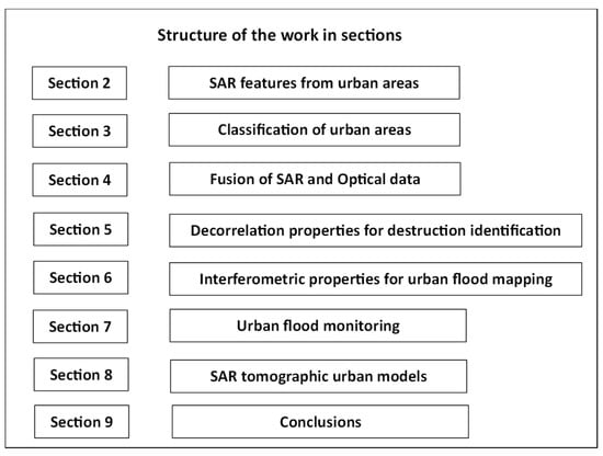
Figure 1.
Block diagram of the organization of the paper in sections.
2. SAR Features from Urban Areas
In this section, two types of features from SAR images for urban region classification are highlighted.
2.1. Textural SAR Features [2]
The objective described in this study is to employ multidimensional textural features as they are expressed by the co-occurrence matrices for distinguishing between various urban environments, following the approach outlined by Dell’Acqua and Gamba [79]. The proposal involves utilizing multiple scales and a training methodology to select the most suitable ones for a specific classification task.
In SAR images, textural characteristics have demonstrated significant promise. In contrast to optical images, SAR images are often affected by speckle noise, rendering individual pixel values unreliable. This underscores the enhanced appeal of textural operators for emphasizing the spatial patterns of backscatterers in SAR images. Utilizing supervised clustering on these features can help identify regions where buildings and other human-made structures exhibit similar patterns. This means that residential areas characterized by isolated scattering elements differ significantly from urban centers with densely packed scattering mechanisms, or commercial districts where strong radar responses are caused by a small number of high buildings.
The problem of region segmentation is very serious when the background is characterized by the stochastic nature of the SAR backscatter. This stochastic nature is the main reason that ordinary segmentation techniques cannot achieve high success in segmentation, especially in an urban environment. Possible solutions for SAR urban segmentation come from high-order statistics, the simplest of which are co-occurrence matrices.
To calculate a co-occurrence matrix, you need to determine how frequently the values i and j co-occur inside a window for a pixel pair with specific relative locations, as depicted in Figure 2. These locations are defined by the horizontal and vertical relative displacements of the two pixels. This is the Cartesian form of displacement. Another way is to express the displacement in vector terms, giving its amplitude and the angle formed with the horizontal direction. Finally, it is very important to consider the size of the squared window as well as the number of quantization levels required to quantize the values of the pixels.

Figure 2.
Evaluation of a co-occurrence matrix. On the left are depicted the pixel values of the gray-tone image. The pixel pair is determined by the vector . The co-occurrence matrix is given on the right of the figure.
It is clear that a significant number of the above parameters are interconnected with scale factors. The unique parameter is irrelevant to the rest is the number of quantization levels, which correspond to the number of bits employed. The evaluation of the co-occurrence matrix is faster as the number of bits is smaller. Conversely, reducing the number of bits results in a greater loss of information. In urban SAR images, the gray-level histogram typically exhibits long tails due to the presence of strong scatterers. These strong scatterers generate exceptionally strong spikes in the images due to dihedral backscattering mechanisms [80], resulting in very high data values. Hence, the initial amplitude floating-point SAR images can be converted into integers with 256 levels prior to performing texture evaluation. The most important parameters are the distance and the direction. Direction becomes particularly crucial when dealing with anisotropic textures that require characterization. The common approach involves joining different directions and calculating the mean value of the textural parameters across these directions. In urban areas, it is important to note that the anisotropy observed in different parts of the scene tends to aggregate into a more general isotropic pattern in coarse-resolution satellite images. In such cases, distance becomes a crucial factor in distinguishing between textures that may consist of identical elements but with varying spatial arrangements.
The final parameter to consider is the extent of the co-occurrence window. It is widely acknowledged that a narrower window is preferable, primarily due to boundary-related concerns. Nevertheless, for precise texture evaluation, a window that changes continuously and gradually, with somewhat loosely defined boundaries, should be chosen. Therefore, the width is the procedural characteristic that only relies on the spatial scale of the environment of a city. In the example depicted in Figure 2, the width is 3 × 1.
The challenge here lies in the fact that the width needs to be evaluated by means of a testing process, and it may not be universally applicable to all images of the same region, incorporating the corresponding data from a multitemporal sequence of images captured by the same sensor. While it is evident that extremely uncommon window dimensions are unsuitable for classification purposes, some values in the vicinity of the chosen 21×21 squared window yield sometimes better results. Using a unique scale for textural processing can certainly diminish the characteristics of the classification map along the neighborhood of the zones, as it disregards evidence present at other scales. However, when multiple scales are considered, it necessitates the analysis of a substantial number of bands. To mitigate this issue, a common approach is to leverage feature space reduction procedures, originally developed for hyperspectral data, such as effective feature extraction via spectral-spatial filter discrimination analysis [81]. These techniques help reduce the dimensionality of the data. In this way, the very crucial textural features at various scales are retained, which serve as inputs to the classifier. Features extracted based on texture as well as multispectral information [81] enrich the information content to be processed in dimensionality reduction approaches.
In the experiments, test SAR data were utilized from the urban region located in Pavia, Northern Italy. The images were sourced from the ASAR sensor onboard the ENVISAT satellite, as well as from ERS-1/2 and RADARSAT-1. To facilitate data examination, a surface truth map was created by visually interpreting the same area with a fine-resolution optical satellite panchromatic image from IKONOS-2 with 1 m spatial resolution, acquired in July 2001. It is worth noting that when classifying using individual sensors, the classification accuracy hovered around 55%. However, combining the data from ENVISAT and ERS sensors proved to be highly successful, resulting in an overall accuracy of 71.5%. This joint use of ENVISAT and ERS data outperformed using ERS data alone, which achieved accuracies of approximately 62%, and also outperformed the classification based solely on the two ASAR images, which achieved an accuracy of 65.4%.
In conclusion, the study presented in [2] demonstrated that the characterization of an urban environment can be significantly enhanced by employing multiscale textural features extracted from satellite SAR data.
2.2. SAR Target Decomposition Features for Urban Areas [10]
Target decomposition parameters represent a highly effective approach for extracting both the geometrical and electrical properties of a target. These parameters are not of the same importance, and the main problems a researcher has to solve are:
- To determine the maximum number of these parameters, as they are derived from various methods.
- To access each of the derived parameters as far as their information content is concerned and to use the most important of them for urban classification.
Both issues are addressed in [10].
Cloude-Pottier’s incoherent target decomposition [82] has emerged as the most widely adopted method for decomposing scattering from natural extended targets. Unlike the Cloude-Pottier decomposition, which characterizes target scattering type with a real parameter known as Cloude , a decomposing technique by Touzi utilizes both the magnitude and the phase of the “complex” scatterer proposed in [83]. This approach provides an unambiguous means for characterizing target scattering. In order to preserve all available information, no averaging of scattering parameters is performed. Instead, target scattering parameters are characterized through a thorough analysis of each of the three eigenvector parameters, resulting in a total of 12 roll-invariant parameters. However, a smaller number of these invariant parameters are necessary for scatterer classification. Accordingly, there is a necessity for a technique for choosing the most meaningful parameters for efficient classification. This ideal subset, obtained by the optimum incoherent target decomposition (ICTD) method, guarantees correct classification without information loss. The selection process is based on mutual information theory, which is extensively detailed in [10]. This paper briefly introduces the Touzi decomposition method, followed by an exploration of Shannon’s mutual information theory. This theory is then applied to rank and select an optimal parameter subset for classifying city regions. Two different methods were introduced for selecting the appropriate parameter subset: the maximum mutual information (MIM) approach and the maximum relevancy and minimum redundancy (MRMR) approach. The two approaches are compared as far as their effectiveness in feature selection and region classification is concerned. The optimal subsets obtained through MIM and MRMR are subsequently utilized for urban site classification, employing support vector machines (SVM). The study uses polarimetric Convair 580 SAR data collected over an urban site in Ottawa, Ontario, to evaluate and assess the results of parameter selection and region classification.
Touzi decomposition, as described in reference [83], relies on the characteristic decomposition of the coherency matrix . In the case of a reciprocal target, this characteristic approach of decomposing the Hermitian-positive semi-definite target coherence matrix gives the possibility of interpreting it as the incoherent sum of up to three coherence matrices . These three matrices represent three distinct single scatterers, and each one is weighted by its respective positive real eigenvalue
Each eigenvector , which is related to a unique scattering mechanism, is represented by the four roll-invariant scattering parameters, as drawn below:
In this context, each individual coherent scatterer is defined by its scattering type, which is described in terms of polar coordinates and , along with the parameter representing the level of symmetry. The eigenvalue , which is normalized, indicates the proportion of energy associated with the scattering mechanism, denoted by the corresponding eigenvector .
The target scattering properties are uniquely characterized by analyzing each of the three eigenvector parameters obtained by the Touzi decomposition.
As described by Shannon [84], entropy, denoted as , serves as the fundamental measure of information, quantifying the uncertainty related to the random variable X. Mutual information, denoted by Shannon as is a metric used to account for both correlation as well as dissimilarity among two random variables and . When selecting among n features, the goal is to maximize the joint mutual information, . Estimating the distribution of , which is of a high dimension, can be quite challenging, and it is often assumed that is independent from all other features for estimating and ordering the features in descending order of importance, especially when we exclusively rely on mutual information criteria for feature selection. The association among the entropies and , as well as the mutual information for two random variables and is illustrated by the Venn diagram in Figure 3.
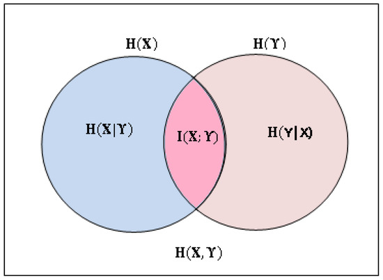
Figure 3.
The Venn diagram is the most suitable tool to demonstrate the association among variables X and Y.
The definition of the entropy , joint entropy , conditional entropy and mutual information of two random variables and , based on their probability density function and joint probability density function is given by Equation (3):
Mutual information quantifies the extent of information shared between two random variables, and . It is important to note that mutual information is nonnegative () and symmetric (). In the context of machine learning and feature selection, mutual information plays a significant role. It can be demonstrated that if X represents the set of input features while represents the target class, then the prediction error for Y based on is confined from below by Fano’s inequality [85]. For any predictor function applied to an input feature set , the lower bound for prediction error is as follows:
while it is bounded from above by Hellman–Raviv’s inequality [86]
According to (5), as the mutual information increases, the prediction error bound becomes minimum. This serves as the primary incentive for employing mutual information criteria for selecting features. The concept becomes even clearer when considering the Venn diagram depicted in Figure 3.
It is important to mention that an ideal set of features has to be individually relevant as well as exhibit minimal redundancy among themselves. As mentioned previously, for each chosen feature , the mutual information was maximized when selecting the required features from the complete feature set. The most straightforward method involves maximizing the mutual information, as defined in Equation (6), and subsequently arranging the features in descending order based on their relevance to the target class :
However, the MIM approach does not provide insights into the mutual relationships between the parameters. In contrast, the MRMR criteria select each new feature based on two key considerations: it should have the individual mutual information as high as possible, and it should contribute the lowest possible joint mutual information or redundancy. The number of preselected features is represented by the variable , and the candidate features by . The MRMR criterion is expressed as:
The features are assessed based on (6) and (7), while the classification of the urban area is carried out using the ranked set of these features. Accordingly, the ranked parameters are examined regarding their relevance to the target classification using the MIM criterion. Furthermore, their redundancy is evaluated in conjunction with preselected parameters using the MRMR criterion. The target classes considered are = {forest, bare ground, small housing, water}. This classification process helps identify which features are most informative and non-redundant for distinguishing between these specific classes in the urban area.
In summary, both the MIM and MRMR methods, which facilitate the ranking and selection of a minimal subset from the extensive set of ICTD parameters, demonstrate their effectiveness in achieving precise image classification. A comparative analysis was conducted to assess the effectiveness of these two approaches in feature selection and their ability to discriminate between classes. The optimal subset, determined through the MIM and MRMR criteria, was utilized for urban site classification using SVMs. The findings suggest that a minimum of eight parameters is necessary to achieve accurate urban feature classification. The chosen parameter set from the ranked features not only enhances our understanding of land use types but also reduces processing time for classification while increasing classification accuracy.
A significant contribution for using the backscattering mechanism of PolSAR data for urban land cover classification and impervious surfaces classification was investigated in [22] and provides similar classification results as the work in [10]. The paper proposes a new classification scheme by defining different land cover subtypes according to their polarimetric backscattering mechanisms. Three scenes of fully polarimetric Radsarsat-2 data in the cities of Shenzhen, Hong Kong, and Macau were employed to test and validate the proposed methodology. Several interesting findings were observed. First, the importance of different polarimetric features and land cover confusions was investigated, and it was indicated that the alpha, entropy, and anisotropy from the H/A/Alpha decomposition were more important than other features. One or two, but not all, components from other decompositions also contributed to the results. The accuracy assessment showed that impervious surface classification using PolSAR data reaches 97.48%.
3. Methods for Urban Area Classification Using SAR [28]
The classification of urban areas using SAR images has the following advantages and disadvantages, which must be considered thoroughly in order to reveal all the information available.
Advantages
- Give day and night images.
- Give images even if the area is covered by clouds.
- Give high-resolution information regarding the geometric and electric properties of the scatterers.
Disadvantages
- They are prone to speckle noise.
- They are affected by moisture and atmospheric conditions.
Different classification approaches give a large variety of performances in distinguishing urban land cover.
Cloud cover remains a persistent problem in the field of optical remote sensing, impeding the seamless and precise monitoring of urban land changes. An examination of more than a decade of ongoing data acquisitions using the Moderate Resolution Imaging Spectrometer (MODIS) revealed that, on average, approximately 67% of the Earth’s surface is cloud-covered [87]. Obtaining cloud-free remote sensing images is a rare occurrence, and this challenge is particularly pronounced in tropical and subtropical regions, which tend to experience frequent cloud cover and rainfall. On the contrary, SAR has emerged as a valuable complement to optical remote sensing, particularly in regions prone to cloud cover, thanks to its all-weather and day-and-night imaging capabilities. Fusion of optical and SAR images has been proposed so far based on various approaches and implemented separately in pixel level, feature level, and decision level fusion [45,88]. Fusing pixels involves directly overlaying optical and SAR data at the pixel level without extracting specific features. However, some studies have suggested that fusing optical and SAR data at the pixel level might not be ideal due to the fundamentally different imaging mechanisms employed by these two sensor types [89]. Merging information at the feature level involves the integration of this information obtained from both optical and SAR data. Most of the multi-sensor fusion techniques focus on merging features due to advanced technological and theoretical progress. Common methods employed for feature-level fusion encompass support vector machines [90], random forest [91], and deep learning techniques [92]. The fusion of decisions, on the other hand, involves classifying land cover by means of visual and SAR images separately and then inferring based on the obtained classification results. Methods for integrating decisions for visual and SAR data typically include techniques such as voting, the Dempster–Shafer theory, and Random Forest [40,93,94].
Indeed, a thorough investigation of the role of SAR in the presence of clouds, particularly its influence on optical images covered mostly by clouds and its impact on separating different land cover types in varying cloud conditions, is an area that requires further exploration. The fundamental question revolves around understanding how clouds precisely affect land cover recognition in urban land cover classification when integrating optical and SAR images. To address this, there is a need for a methodology to examine the mechanisms through which clouds affect urban land cover classification and allow for the quantification of the supplementary benefit of SAR data.
The area for exploitation is the Pearl River Delta in southern China. The methodology followed in this study comprises a novel sampling strategy aimed at extracting samples with varying degrees of cloud cover and constructing a dataset that allows for the quantitative assessment of the impact of cloud content on the analysis. Accordingly, both the optical and SAR images were subjected to individual preprocessing steps using appropriate techniques. Subsequently, these images were co-registered to ensure proper alignment. After co-registration, different features were used from the co-registered visual and SAR data. These extracted features would serve as the basis for further analysis and evaluation of land cover classification, taking into account cloud content variations. For the specific levels of cloud coverage, the three representative classifiers were employed to perform the urban land cover classification. Subsequently, validation procedures and accuracy assessments were conducted to evaluate the influence of cloud cover and assess the additional value of SAR data in discriminating between land cover categories (Figure 4).
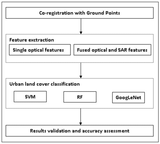
Figure 4.
The methodology followed in this work comprises the three different tested classification schemes.
Different feature extraction phases were employed to acquire information from optical and SAR data. Preprocessing comes first before geocoding and co-registering the ALOS-2 with the Sentinel-2 data. In order not to destroy textural information, calibration and speckle noise reduction are first performed. After that, the ALOS-2 data and the polarimetric features are geocoded and co-registered with the Sentinel-2 images.
In the analysis, the set of optical features employed the original spectral signatures, the normalized difference vegetation index, and the normalized difference water index. In addition to these spectral features, textural information was extracted using the four features inherent in the gray-level co-occurrence matrix. Namely homogeneity, dissimilarity, entropy, and the angular second moment. Thus, a total of 12 × 4 feature layers were acquired. To reduce dimensionality, principal component analysis was applied, resulting in a final set of 18 optical feature layers. Features from SAR data were engaged to enhance the discrimination of different land cover types, particularly in the presence of cloud cover. Specifically, the backscattering polarization components HH, HV, VH, and VV, the polarization ratio, the coherence coefficient as well as the Freeman–Durden decomposition parameters [95], the Cloude–Pottier decomposition parameters [96] and the Yamaguchi four-component decomposition parameters [97] were employed. Optical and SAR features stacked together constitute a 44-dimensional feature vector. Normalization of the features is necessary to avoid potential biases.
To assess the effect of clouds on classifying land types, three distinct classification approaches were utilized:
- Support vector machine (SVM);
- Random forest;
- The typical supervised machine learning method.
These three classification algorithms were chosen due to their stable and well-documented performance in various classification tasks.
The SVM classifier operates by creating a decision boundary, often described as the “best separating hyperplane”, with the objective of maximizing the margin between two distinct classes or groups. This hyperplane is located within the n-dimensional classification space, where “n” represents the number of feature bands or dimensions. The SVM algorithm iteratively identifies patterns in the training data and determines the optimal hyperplane boundary that best separates the classes. This configuration is then applied to a different dataset for classification. In the context of this work, the dimensions of the classification space correspond to the available bands, while the separate pixels within a multiband image are represented by vectors.
The random forest training approach was proposed by Breiman in 2001 [91] since the grouping of aggregated classifiers outperforms a single classifier. Each decision tree is constructed when training samples are randomly selected and are called out-of-bag samples [98]. These samples can be fed to the decision tree for testing, which helps to de-correlate the trees and consequently reduce multicollinearity. Accordingly, different decision trees can be formed by means of different organization of the input data so that to build the random forest classifier.
GoogLeNet [99] is a very well-known deep convolutional neural network with 22 layers that was developed by Google. One of its significant contributions is the introduction of the inception architecture, which is based on the concept of using filters of different sizes in parallel convolutional layers. GoogLeNet, with its prototype architecture, was a substantial advancement in the field of deep learning and convolutional neural networks. It demonstrated that deep networks could be designed to be both accurate and computationally efficient, making them a valuable architecture for a wide range of computer vision tasks.
In order to investigate the performance of classifying land cover types under various percentages of cloud content, the study required datasets with different cloud contents. The key details about the dataset used for this purpose are the total of 43,665 labeled pixels representing five different land cover classes (vegetation (VEG), soil (SOI), bright impervious surface (BIS), dark impervious surface (DIS) and water (WAT)). Visual interpretation was carried out for labeling the above pixels. For the experiments, the 43,665 classified pixels in the specific image were employed to develop the dataset with specific cloud coverage (0, 6%, 30%, and 50%). The respective number of pixels is encountered when the cloud content corresponds to each of the above four cloud coverages. Each time, half of the pixels were randomly selected as training samples, and the other half were selected as testing.
Quantitative metrics, including the standard accuracy metrics of the overall accuracy, the confusion matrix, the producer’s accuracy, and the user’s accuracy, were employed to evaluate the results. Furthermore, two different assessment methods were employed to evaluate the effects of clouds on urban land cover classification, namely the overall accuracy to quantify the influences of different percentages of clouds on classification and the evaluation of the confusion of land covers under cloud-free and cloud-covered areas.
In general, the performance of this approach [28] is similar to other approaches in the literature, such as those in Refs [45,88,94]. These techniques present a combination of classification methods to improve the final urban identification performance.
4. Fusion Techniques of SAR and Optical Data for Urban Regions Characterization [40]
Fusion of different remotely sensed images of the same areas is very essential for improving land cover classification and object identification. Fusion techniques are intended to solve three main issues in land classification procedures.
- Combining mainly optical, thermal and radar (SAR) images in order to extract special information from each of these EM scatterings.
- Cover with complementary information land regions for which some of the data are missing (i.e., optical information obscured by cloud cover).
- Fused information at the pixel level, employing, if necessary, decision fusion techniques in order to decide about the type of land cover in fine resolution analysis.
Impervious surfaces refer to human-made features such as building rooftops, concrete, and pavement that do not allow water to penetrate the soil. They are crucial indicators in assessing urbanization and ecological environments. The increase in impervious surfaces can lead to various environmental challenges, including reduced green areas, water pollution, and the exacerbation of the urban heat island effect [100]. For the time being, medium/coarse-spatial resolution satellite images were used to calculate impervious surfaces [101,102,103].
Despite the existence of various mapping techniques, the majority of them were originally developed with a focus on optical imagery. The wide range of urban land covers, including those with similar spectral characteristics, makes it challenging to precisely assess impervious surfaces using optical images. To illustrate, there have been instances where water and shaded areas have been mistakenly identified as dark impervious surfaces. Consequently, the practice of fusing remotely sensed images from various sources was employed to capitalize on the unique attributes of different images with the aim of enhancing mapping accuracy [104]. Prior investigations have demonstrated that combining optical and SAR data can notably enhance image classification accuracy while also diminishing the potential for misidentifying urban impervious surfaces and other land cover categories. SAR data exhibits sensitivity to the geometric attributes of urban land surfaces, offering valuable supplementary information regarding shape and texture. It has been recognized as a significant data source when used in conjunction with visual images to characterize impervious surfaces.
Presently, the fusion of visual and SAR images for unaffected surface mapping primarily occurs at pixel and feature levels. Nevertheless, pixel-level fusion encounters challenges with SAR images due to speckle noise, making it less suitable [105]. Moreover, feature-level fusion is susceptible to the effects of feature selection, potentially introducing ambiguities in classifying impervious surfaces. In this study, fusion of decisions pertains to the merging of classification outcomes originating from various data sources, such as optical or SAR data, in order to arrive at a conclusive land cover type determination for a given pixel. Leveraging the Dempster–Shafer (D-S) evidence theory [106,107], decision-level fusion has demonstrated promise as a possibly appropriate approach for classifying land cover types, despite being relatively underexplored in previous research. Fusing the classification outcomes from diverse data sources has exhibited advantages in image classification when compared to conventional Bayesian methods [108,109]. The D-S evidence theory considers unaffected surface estimations obtained from various data sources as independent indications and introduces measures of uncertainty for the combined unaffected surface datasets. Hence, the primary goal is to generate a precise urban impervious surface map through the decision-level integration of GF-1 and Sentinel-1A data, employing the Dempster–Shafer (D-S) theory. Additionally, this approach aims to offer in-depth assessments of the levels of uncertainty associated with impervious surface estimations. Initially, different land categories were individually classified from GF-1 (GaoFen-1 satellite) and Sentinel-1A data using the random forest (RF) methodology. Subsequently, these classifications were combined using the D-S fusion rules. Next, the types of land categories were additionally separated into two groups: non-impervious surfaces and impervious surfaces. To evaluate the accuracy of the estimations, a comparison was made between the estimated impervious surfaces and reference data gathered from Google Earth imagery. The surface under investigation encompasses the city of Wuhan, situated in the eastern Jianghan Plain. This area experiences a tropical humid climate characterized by substantial rainfall and distinct seasonal changes, with four clearly defined seasons.
The process of fusing visual and SAR data based on decisions to evaluate urban unaffected surfaces was executed using the random forest classifier and evidence theory. Additionally, an analysis of the ambiguity levels for these impervious surfaces was conducted. Four key steps were undertaken to fuse visual and SAR images based on decisions. In the initial step, preprocessing was applied to ensure that both visual and SAR data were co-registered. Secondly, the extraction of spectral and textural characteristics from the GF-1 and Sentinel-1A images, respectively, was performed. Subsequently, unaffected surfaces were determined using the random forest classifier, employing data from four distinct sources. Finally, the unaffected surfaces described by these separate datasets were merged using the Dempster–Shafer theory. Figure 5 illustrates both the feature extraction phase and the decision fusion phase.

Figure 5.
The feature extraction step and the decision fusion step. Urban impervious surfaces can be obtained by fusing optical and SAR data.
Texture features are a set of measurements designed to quantify how colors or intensities are spatially arranged in an image. These features are highly important when interpreting SAR data for land cover classification and can be formed by means of the gray-level co-occurrence matrix, which was engaged to acquire textural information from Sentinel-1A images [110]. Additionally, spectral features, i.e., NDVI and NDWI, were obtained from GF-1 imagery and serve as an indicator of vegetation growth and to identify water areas, respectively. This fusion of information enhances the accuracy of land cover classification by capturing both the spatial patterns and spectral characteristics of the Earth’s surface.
The two quantities are evaluated as follows:
where R, G, and NIR correspond to the surface reflectivity in the red, green, and near-infrared spectral bands, respectively.
The random forest algorithm was initially developed as an extension of the decision tree classification model [12,91]. Then, grouping is carried out by building k decision trees (k is user-defined) using the selected N samples. As each decision tree produces a classification result, the ultimate classifier output is decided by taking into account the majority vote from all the decision trees [91,111]. The integration of urban unaffected surfaces from various datasets was carried out at the decision level, employing the Dempster–Shafer theory [107]. In the context of this theory, impervious surface estimations obtained from different satellite sensors are treated as unrelated pieces of proof, and the approach introduces considerations of ambiguity.
In summary, unaffected surfaces were created by combining formerly assessed unaffected surfaces obtained from separate image sources using the Dempster–Shafer fusion rules. Evaluation of the accuracy revealed that unaffected surfaces from urban regions derived from visual data achieved an improved classification performance of 89.68% compared to those derived from SAR data, which achieved a classification accuracy of 68.80%. The fusion of feature information with visual (or SAR) data improved the total classification performance by 2.64% (or 5.90%). Furthermore, the integration of unaffected surface datasets obtained from both GF-1 and Sentinel-1A data led to a substantial enhancement in overall classification accuracy, reaching 93.37%. When additional spectral and texture features were incorporated, the overall classification accuracy further improved to 95.33%.
Further reading with the presentation of various fusion methods as well as performance comparisons can be found in [104]. The procedures presented there are mainly based on pixel-level fusion and decision fusion.
5. Decorrelation Properties for Urban Destruction Identification [49]
One of the approaches used to determine building changes caused by disaster damage is to employ suitable scattering mechanisms and decomposition models and apply them to PolSAR data [112]. As anticipated, the polarimetric features derived from PolSAR data exhibit significant potential for detecting and assessing damaged areas. In the case of low-resolution polarimetric SAR images, which are well-suited for extensive injury assessment over large areas, the primary alterations observed in damaged urban areas involve a decrease in ground-wall structures. The destruction of these structures results in a decrease in the prevalent double-bounce scattering mechanism and disrupts the homogeneity of polarization orientation angles [113]. Two polarimetric damage indexes, developed through in-depth analysis of target scattering mechanisms, have proven effective in distinguishing urban areas with varying degrees of damage.
Consequently, the approach described in this section is intended to give solutions to the following problems:
- Determining changes in buildings caused by disaster damage in urban areas.
- Determining the decrease in ground-wall structures.
- Finding the appropriate indexes to distinguish among various degrees of damage.
Except for the features based on the polarimetric behavior of scattering mechanisms, the cross-channel polarimetric correlation is a crucial resource that holds the potential to unveil the physical characteristics of the observed scene [114]. The magnitude of the polarimetric correlation coefficient, often referred to as polarimetric coherence, has been employed in the examination of PolSAR data. Polarimetric coherence is significantly influenced by factors such as the chosen polarization combination, the local scatterer type, and the orientation of the target relative to the direction of PolSAR illumination. To comprehensively describe the rotation properties of polarimetric matrices, a uniform polarimetric matrix rotation theory was recently developed [115].
The examination of buildings before and after undergoing collapse damage is feasible because the primary distinction between an unharmed building and a collapsed one (which exhibits a rough surface) lies in the alteration of the ground-wall structure. The varying geometries of ground-wall structures and rough surfaces lead to significantly altered directional effects in the rotation domain along the radar’s line of sight. The effects related to directivity and stemming from ground-wall structures are considerably more pronounced compared to those arising from hard surfaces. As a result, the patterns related to polarimetric coherence and corresponding to buildings before and after destruction exhibit discernible differences, making them distinguishable from each other. Furthermore, ground-wall structures and rough surfaces primarily manifest double-bounce and odd-bounce scatterers, which are clearly associated with the combination of co-polarization components as seen in Pauli decomposition. A novel approach for urban damage assessment is being explored, and its uniqueness lies in the fact that it is not influenced by target orientation effects.
In PolSAR, the data acquired on a two-directional basis (horizontal and vertical—H, V polarizations) can be represented in the form of a scattering matrix, which is typically expressed as:
where the subscripts denote the transmitting and the receiving polarizations. If we want to transform the scattering matrix in the direction along the radar line of sight, we follow the relationship:
The superscript † represents the conjugate transpose, and the rotation matrix is
If the co-polarization components are combined in pairs as and , respectively, then we associate them with canonical surface scattering and double-bounce scattering according to Pauli decomposition logic. Accordingly, the co-polarization components and constitute the importance in the next explorations and their representations in the rotation domain are:
Polarimetric coherence can be expressed as the average of sufficient samples with similar behavior [114]. The coherence of co-polarization if rotation is not considered is:
where is the conjugate of , and denotes averaging over the available samples. The value of lies in the interval [0, 1].
The polarimetric coherence pattern [116] is highly effective for understanding, visualizing, and describing polarimetric coherence properties in the rotation field. In this context, the concept of co-polarization coherence pattern is defined as follows:
It is worth mentioning that the rotation angle includes the full range of the rotation domain. If the speckle is significantly eliminated through the estimation process, the co-polarization coherence has a rotation imprint that is totally defined by the elements and . Furthermore, the period of in the rotation field is found to be .
The primary distinction between an unharmed building and a collapsed one lies in the alteration of the ground-wall formation. Notably, the structural characteristics of a rough surface and a dihedral corner reflector, usually employed for modeling a building’s ground-wall structure, are significantly dissimilar. Consequently, their polarimetric coherence imprints in the rotation field can be distinguished from one another. Flat surfaces, theoretically, may exhibit roll-invariance, resulting in minimal co-polarization coherence fluctuations in the rotation field. On the other hand, dihedral structures display evident directivity effects, leading to distinct co-polarization coherence patterns.
The co-polarization coherence fluctuation is defined as:
where corresponds to the standard deviation. The calculation of the co-polarization coherence fluctuations are performed for the full scene. The quantities for the buildings are quite large compared to those from rough surfaces, a fact that is consistent with the previous analysis.
The urban damage index was evaluated using data from the significant Great East Japan earthquake and the subsequent tsunami, which caused extensive damage to coastal areas [117]. The study focuses on the Miyagi prefecture, one of the severely affected regions, for investigation. Multitemporal ALOS/PALSAR PolSAR datasets were collected, co-registered, and utilized for analysis. These datasets underwent an eight-look multi-looking process in the direction of azimuth to ensure consistent pixel sizes in both the azimuth and range directions. This uniformity facilitated comparisons between the corresponding PolSAR and visual images. After that, the SimiTest filter [118], applied with a 15 × 15 moving window, was used to mitigate speckle effects and calculate co-polarization coherence. In the case of flooded urban areas where there is minimal destruction of ground-wall structures, it is evident that the co-polarization coherence patterns, represented as , largely remain consistent before and after the event. These patterns typically exhibit shapes with four-lobes with significant coherence variations. Consequently, the co-polarization variation of the coherence, denoted as , tends to decrease for harmed urban patches after the destruction. Furthermore, the changes in coherence fluctuation, , can also serve as an indicator of the damage degree within the affected regions. As the extent of damage increases, the alterations in coherence fluctuation, become more pronounced, offering the potential to discriminate between different levels of urban damage.
The alterations in the two primary scattering mechanisms, namely, double-bounce scattering and ground-wall structures, are primarily manifested in changes to the co-polarization components and . These changes, in turn, result in different co-polarization coherence patterns in the rotation domain. For intact buildings, the ground-wall structure can be effectively represented by a dihedral corner reflector, which exhibits narrow directivity in the rotation domain. In contrast, for damaged buildings, the areas where the ground-wall structure has been compromised transform into rough surfaces. The directivity of rough surfaces is less sensitive compared to that of a dihedral corner reflector. Consequently, the fluctuation of co-polarization coherence, denoted as , decreases after damage occurs to urban patches. This reduction has the potential to reveal the changes that have taken place in these urban areas before and after the damaging event.
The co-polarization coherence variability, denoted as , represents the standard deviation of coherence values in the rotation field. To designate the coherence fluctuation imprint, it is calculated using the urban mask provided in [18]. When compared with the data before the destruction, the values of co-polarization coherence variability, , noticeably decrease over the damaged regions in the post-event scenario. Furthermore, as anticipated, the extent of the decrease in is closely related to the degree of damage observed in local urban regions. In order to emphasize this association, a damage index indicating the level of urban damage is proposed. This index is defined as the ratio of co-polarization coherence fluctuation before and after the damage event, as shown in the following equation:
where and correspond to pre- and post-destruction, respectively. For intact urban regions, the damage index is close to 1, while for destroyed regions, the index is more than 1.
Quantitative comparisons were conducted for ten selected destroyed urban areas and five urban segments affected by flooding. A 3 × 3 local window was employed to calculate the mean and the standard deviation of the proposed damage index . For the destroyed urban regions, it is evident that the index gets larger as the damage levels escalate. On the other hand, for the urban patches solely affected by flooding, the values of this index consistently remain around 1, indicating an undamaged condition. This aligns with the ground-truth data.
A fourth-order polynomial model is employed for fitting to form the analytical inversion relationship:
where is the destroyed urban degree, , and are weighting parameters. By employing the damage index defined in Equation (17) and the damage level inversion relationship given in Equation (18), an urban damage level mapping procedure has been developed. The flowchart illustrating this approach is presented in Figure 6.
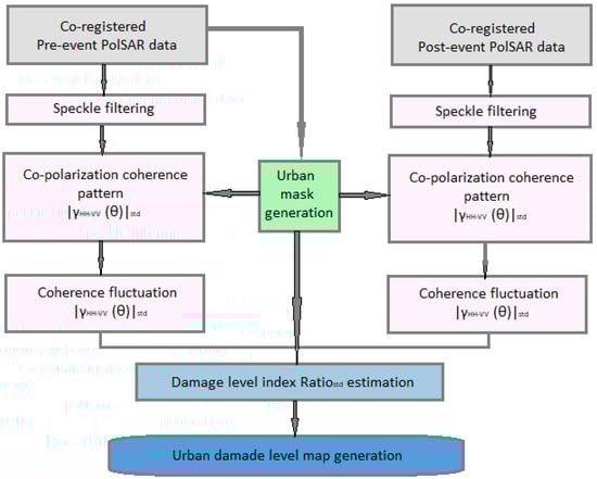
Figure 6.
Block diagram depicting the evaluation of urban damage level mapping.
The damage level inversion relationship gives an urban damage level map covering the entire scene. This approach provides information on both the areas affected by damage and the specific levels of damage within those regions. Experiments have proven the effectiveness of this method, particularly in successfully identifying urban pieces with over 20% damage.
Other methods achieve similar classification performance as far as destruction areas are concerned. According to the scattering interpretation theory [107], a built-up area should respond to dominant double-bounce scattering induced by the ground-wall structures before the damage. However, after the tsunami, most of these buildings were swept away, and the ground-wall structures dramatically decreased. Therefore, this seriously damaged area should obviously be changed into dominant odd-bounce (surface) scattering. Damage level indexes developed from polarimetric scattering mechanism analysis techniques can be more robust than those based on intensity changes [113]. Two indicators from model-based decomposition and PO angle analysis are developed and examined in this work. A classification scheme [116] based on the combination of two kinds of features is established for quantitative investigation and application demonstration. Comparison studies with both UAVSAR and AIRSAR PolSAR data clearly demonstrate the importance and advantage of this combination for land cover classification. The classification accuracy presented in this work was 94.6%. A few examples of detection, determination, and evaluation of the damage to areas affected by the March 11th earthquake and tsunami in East Japan are given in [117]. They show the very promising potential of PolSAR for disaster observation. Detection of damaged areas can be done with only a single PolSAR observation after the disaster.
6. Interferometric Properties for Urban Flood Mapping [55]
In this work, interferometry and coherency are the main tools to distinguish flooded urban areas. This is coming from the basic electromagnetic properties of the PolSAR component (HH, HV, VH, and VV) to reflect in various kinds of areas and land covers.
Flooding is a pervasive and impactful natural disaster that has far-reaching effects on human lives, infrastructure, economies, and local ecosystems. Remote sensing data plays a pivotal role by providing a comprehensive view of large areas in a systematic manner, offering valuable insights into the extent and dynamics of floods. SAR sensors stand out as one of the most commonly used Earth observation sources for flood mapping, thanks to their ability to operate in all weather conditions and provide day–night imaging capabilities. The proliferation of SAR satellite missions has significantly reduced revisit periods and streamlined the process of rapidly mapping floods, particularly in the framework of emergency response attempts.
SAR-based flood mapping has been extensively studied and applied in rural areas [55]. The specular reflection that occurs on smooth water surfaces creates a dark appearance in SAR data, enabling floodwaters to be distinguished from dry land surfaces. In city regions with low slopes and a high proportion of unaffected surfaces, the vulnerability to flooding increases, posing significant risks to human lives and economic infrastructure. Thus, flood detection in urban areas presents considerable challenges for SAR because of complicated backscatterers associated with diverse building types and heights, vegetated areas, and varying road network topologies.
Several research studies have provided evidence that SAR interferometric coherence (γ) is a valuable source of information for urban flood mapping and can be instrumental in addressing specific challenges [119]. Urban areas are generally considered stable targets with high coherence properties. When it comes to the decorrelation of coherence, it is typically influenced more by the spatial separation between successive satellite orbits than the time gap between two SAR acquisitions [120]. The spatial distribution of scatterers within a resolution cell can be disrupted by the presence of standing floodwater between buildings. This disturbance leads to a reduction in the coherence of co-event pairs compared to pre-event pairs, making it possible to detect and map urban floods based on changes in coherence. In reference [55], a method is proposed for detecting floods in urban settings by utilizing SAR intensity and coherence data through Bayesian network fusion. This approach harnesses time series information from SAR intensity and coherence to map three key areas: non-obstructed-flooded regions, obstructed-flooded non-coherent areas, and obstructed-flooded coherent areas. What makes this method unique is its incorporation of the stability of scatterers in urban areas when merging intensity and coherence data. Additionally, the threshold values used in the process are understood directly from the data, giving a procedure that is automatic and independent of specific sensors as well as the regions under investigation.
A Bayesian network is a probabilistic graphical model that provides a concise representation of the joint probability distribution of a predefined set of random variables. It is depicted as a directed acyclic graph (DAG), with nodes representing variables and links between nodes indicating dependencies among these variables [121]. The DAG explicitly defines conditional independence relationships among variables with respect to their ancestors. Assuming represent the random variables, the joint probability distribution within a Bayesian network can be expressed as follows:
where represent the parent variables of . An arrow will show the direction from the parent to the child variable in the DAG. The Bayesian network offers insights into the underlying process, enabling the expression of conditional distributions through inference. The Bayesian network created for flood mapping incorporates data from backscatter intensity and interferometric coherence time series. The structure of this network is illustrated in Figure 7a. In Figure 7, the shaded nodes represent observed variables, while the open nodes represent unknown variables. Specifically, the random variable F represents the flood state, with 1 for flood and 0 for non-flood state for each pixel. This variable is the point of interest for which the posterior probability is to be inferred based on all the other variables in the network. The variable D symbolizes the fusion of intensity and coherence time series, specifically, the composite imagery consisting of multitemporal intensity and coherence data. On the other hand, C is a hidden variable that serves as a link, capturing the effect of variable F on the recorded image series D. Determining a direct cause-and-effect relationship between the flood condition and the observed SAR characteristics can be difficult, particularly in urban regions where complex backscattering mechanisms arise from diverse land cover types. Hence, it becomes fundamental to initiate an intermediate variable C with K potential states, each representing distinct temporal behaviors of the area under consideration. These states correspond to different land covers when viewed through SAR data, encompassing both intensity and coherence characteristics [122]. Intensity and coherence are two SAR data properties that capture different physical characteristics of a scene. Intensity provides insights into surface roughness and permittivity, while coherence measures the random fluctuations of individual scatterers between two SAR acquisitions, indicating the temporal consistency within a specific cell.
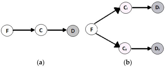
Figure 7.
Flood mapping as represented by a Bayesian network structure. denotes flood states, is a hidden variable, and represents the SAR data. Subscripts and denote intensity and coherence. (a) The initial structure. (b) Structure with dissociated variables and .
Considering this fact, the hidden variable C is split into two variables, namely and , corresponding to the temporal signatures of intensity and coherence (as shown in Figure 7b). This division enables the evaluation of the flood state for a particular class , from both the intensity perspective (e.g., and the coherence perspective (e.g., . The variable D is partitioned into two components: intensity () and coherence series (. The segmentation of land cover () is carried out based on the combined analysis of the intensity and coherence time series (variable ). This approach ensures that the intrinsic relationships between these two data channels are considered, allowing for the preservation of compact clusters within the area of interest.
The joint probability of from Figure 7b is:
and the posterior probability of can be expressed as:
where and can be evaluated by means of the Bayes rule:
with .
The terms in (21) can be analytically evaluated. The distribution of is calculated using a finite Gaussian mixture model which contains the hidden variable . Each assignment of is a Gaussian component; thus, , and the parameters of each Gaussian component, , are evaluated by employing the expectation-maximization algorithm [123]. Therefore, and are also Gaussian densities and can be evaluated by and , respectively [116]. The number of Gaussian mixtures, , depends on the homogeneity of the area of interest. A homogeneous area requires a smaller value of .
In Equation (22), the term represents the weighting vector associated with Gaussian elements. Meanwhile, is a conditional probability table that has the flood probability for each of these components. This conditional probability table is a pivotal element of the entire process, as it fundamentally influences the final outcome. The estimation of this conditional probability table relies on the assumption that the presence of floodwater can result in a sudden alteration in either intensity or coherence. To calculate the probabilities, the table is built on the variation between the average of the pre-event series and the co-event acquisition for each component centroid (e.g., , and ). Let be the variation vector for which we are interested in:
where and correspond to the respective values of two vectors, is the average towards the time axis, and are the centroids of the pre-event series and the co-event acquisition, respectively. The conditional probability is described by the sigmoid function as follows:
where is the steepness of the curve, and is the value at
Consequently, the classification of the area of interest into coherent (built-up) and non-coherent (empty) regions by means of the relationship between and a threshold comes first, and afterwards, and are refined as:
where represents the logical AND, and stands for the logical OR. Equation (25) adjusts the flood proof based on intensity and coherence, considering each component’s category. For components in built-up areas (coherent), when the flood proof relies mainly on coherence () but not on intensity (), suggesting intensity may not indicate flooding effectively. In such cases, a probability of is assigned to this component, reflecting intensity’s uncertainty in detecting flooding.
Conclusively, this work [55] presents a technique for mapping floods in city areas using SAR intensity and interferometric coherence within the Bayesian network fusion framework. It combines intensity and coherence data probabilistically and accounts for flood uncertainty related to both intensity and coherence. This approach effectively gets flood information across diverse types of land cover and provides maps indicating both the coverage and type of flooding.
The main limitations of the method lie in data availability and scalability. Although the method is flexible in terms of data availability, both (long) time series or bi-temporal data can be used; a longer time series produces more unbiased coherent-area estimation and subsequently achieves a better conditional probability table (CPT). For satellite missions with irregular observation scenarios such as ALOS-2/PALSAR-2 and TerraSAR-X, it can be hard to achieve a long time series of images with consistent acquisition parameters. Nevertheless, this does not mean that the method will fail to succeed with less multi-temporal data, as shown in the Joso case of this study. Promising results are achieved with less than five coherence sequences. Data acquisition is going to be a less crucial problem with the evolution of SAR missions. Satellite constellations such as the Sentinel-1 mission and the recently launched RADARSAT Constellation Mission with high temporal resolution can provide a long and dense observation sequence of an area of interest, and upcoming missions such as Tandem-L and NASA-ISRO SAR (NISAR) will increase the observation frequency of space-borne SAR systems at the global scale.
7. Flood Detection in Urban Areas Using Multitemporal SAR Data [58]
The main goal of this discipline is to develop methods and techniques for creating flood models that are able to model the extent of the flood as well as, according to movement equations, its future extent and lurking danger.
Contemporary real-time flood prediction models are employed for early public warnings. However, these models often lack precise quantification of inherent uncertainties for end-users [124]. One significant source of ambiguity in accumulation models relates to topography data. Airborne light detection and ranging (LiDAR) and Earth-observing satellites are becoming increasingly valuable resources for obtaining precise topographical data in large-scale models [125]. Thinking of universal approaches, digital elevation models (DEMs) derived from remote sensed data offer a smart replacement to airborne LiDAR DEMs, which face limitations in terms of global availability and cost [126].
Global-scale flood mapping belongs to the large-scale flood models [127], which are essential for providing accurate and current flood protection information. One potential solution is to identify the locations of flood defense features using satellite imagery. While SAR satellites offer clear advantages in tracking the spatiotemporal water flow, vegetation can obscure the detection of water edges by scattering the return signal. There is a growing need for flood defense information to enhance flood models, particularly in areas that are difficult to access or lack extensive data, or when dealing with vast geographical areas. The goal here is to pinpoint flood edges by utilizing sequential SAR images in conjunction with water level measurements from gauging stations. The underlying principle of this approach is that once the flood boundary reaches the toe of the embankment, it remains consistent across a range of water levels.
Multi-temporal satellite observations can be employed to map the expansion and contraction of floods. The extent of the flood is linked to the distance between the center of the river and the flood edge. The method introduced in [58] involves determining a stage-extent relationship for a given cross section. This methodology utilizes these stage-extent relationships and systematically seeks long horizontal lines at each cross section to determine the position of flood banks. The method can be divided into two parts, as illustrated in Figure 8: Part 1 of the process focuses on the manipulation of SAR imagery to create fluvial flood maps, which outline the regions submerged by river water. Part 2 outlines the steps for implementing the stage-extent plot and using it to identify the positions of embankments along specified cross sections.
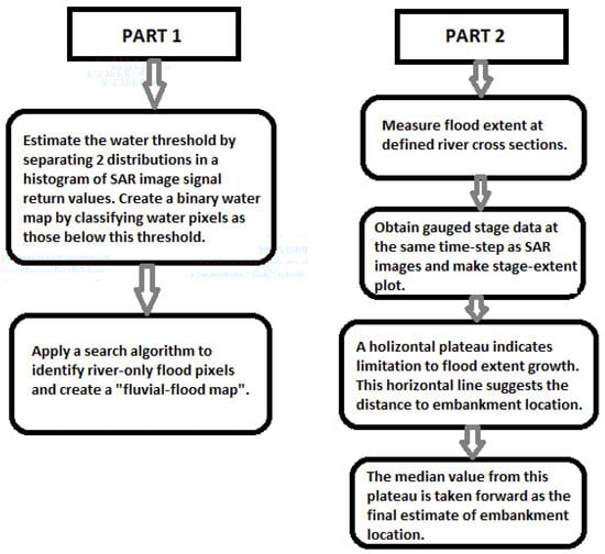
Figure 8.
Key steps within the methodology in [58].
Time series of SAR data are valuable for mapping flood extent due to the pronounced texture difference in SAR images concerning flat water surfaces and rougher land regions. To determine river flood extent, a two-stage classification approach was employed. In Part 1a, gray-level thresholding was utilized, a method commonly employed in previous flood mapping algorithms. In SAR imagery, smooth water typically appears dark because of specular reflection, while rougher vegetation and land cover scatter a larger portion of the radar return to the satellite sensor, resulting in a lighter appearance. Histogram thresholding helps to determine water pixels within a SAR image based on the distribution of these pixels. However, this can be challenging as water and land distributions often overlap.
Only values less than the 99th percentile and larger than the 1st percentile on the y-axis from this fit were maintained. This rejection was done to address the issue of extremely small values. Afterward, the resulting histogram was modified to have a maximum value of one on the y-axis. It was consistently observed that the x-axis value (backscatter in dB) corresponding to 0.01 on the y-axis value of the fitted histogram served as a reliable assessment of the water threshold. The water map that emerged from this estimation closely matched the visually projected flood extent, which was derived from flood levels assessed in comparison to DEM data.
In the context of embankment detection, the primary focus was on the area flooded by river water. To achieve this, water resulting from ponding was excluded. This process involved removing ponding water from the initial binary water map, resulting in what we term a “fluvial flood map.” To create the fluvial flood map for Part 1b, a spread operation that commenced at the river center was employed. In the stage-extent plots used for embankment detection, cross sections vertical to the river’s axis were generated, as illustrated in Figure 8. These fluvial flood maps preserved the same pixel size as the original SAR images. To measure the flood area, the distances between the river center pixels and the pixels from the flood edges were calculated. The flood edge was identified as the farthest water pixel from the river center line along the cross section. It is important to note that both the binary water map and the associated fluvial flood map are sensitive to the chosen water threshold value in the SAR imagery. Therefore, testing was conducted using a range of threshold values, and the positional error was assessed in relation to the selected threshold value.
In conclusion, hydrodynamic models and flood management plans often encounter challenges in getting accurate data on embankment location and height. These challenges can arise due to difficulties related to location, scale, or cost. One effective approach to minimizing errors is to exclude vegetated regions, which means avoiding the placement of cross sections on areas with light signal returns in a SAR image. The works in [128,129] present very recent results in the performance of modern flood defense systems, which are very effective in flood disaster regions.
8. SAR Tomographic Urban Models
In this section, two approaches to urban SAR tomography that have been presented in the literature are highlighted.
In the first case, the prerequisites to build a tomographic SAR image are:
- -
- Scatterers at different elevation positions must be contained.
- -
- Moving scatterers at the same pixels must be resolved.
- -
- The elevation resolution must be determined.
In the second case:
- -
- A synthetic aperture in elevation through a series of multi-baseline interferometric images is created.
- -
- Distinguishing between reliable scatterers and false alarms is a significant challenge.
- -
- Sparse sampling in the elevation direction can lead to ambiguities.
8.1. Super-Resolution for Tomographic SAR Imaging in Urban Areas [65]
In urban environments, one of the primary challenges is addressing layover, which involves detecting multiple distinct scatterers within a pixel. Here, the word “pixel” represents a pixel in the azimuth direction, and it is considered to contain multiple scatterers at different elevation positions. To tackle this issue, TomoSAR techniques have been applied to C-band European Remote Sensing (ERS) satellite data. Resolving discrete scatterers that may also exhibit motion is often referred to as D-TomoSAR or 4-D SAR focusing. The objective is not only to distinguish targets that interfere within the same pixel in the azimuth direction but also to assess any possible relative motion among them. The methodology outlined in [130] introduced an approach for extracting time series of displacement. This method is capable of capturing the displacement patterns for both individual scatterers and for pairs of interfering scatterers. It hinges on the utilization of the velocity spectrum.
Tomographic SAR inversion can be understood as a spectral estimation problem. The Rayleigh elevation resolution is determined as follows [63]:
In the equation, λ represents the wavelength, and △b corresponds to the altitude aperture size, which signifies the width of orbit tracks vertical to the line-of-sight direction. In modern SAR satellites, there is a need for a compact orbital tube, primarily for differential interferometric SAR (D-InSAR) applications. As a result, the altitude aperture tends to be small, leading to a Rayleigh resolution in altitude that is typically approximately 50 times less precise than in azimuth or range.
Only two scatterers are able to separate linear reconstruction methods when their altitude distance () is greater than or equal to the elevation resolution (). However, parametric or nonparametric methods that prioritize sparse solutions offer the potential for super resolution (SR), which can resolve scatterers even when is less than . In a study [18], the authors introduced a super-resolving approach created to minimize the norm, which they named “Scale-down by norm Minimization, Model selection, and Estimation Reconstruction” (SL1MMER, pronounced “slimmer”). In another investigation [131], they explored the SR capabilities and estimation precision of this approach for discriminating scatterers, which are very close with . They approached the SR problem as a detection procedure, defining the altitude resolution as the minimum distance between two scatterers that can be distinguished with a 50% probability of detection. They also introduced the SR factor , defined as:
In [131], it was proved that:
- The super resolution factor of SL1MMER varies asymptotically on the product of the number of acquisitions N as well as on the signal-to-noise ratio (SNR).
- Not uniform aperture sampling does not significantly influence the super resolution.
- The detection success varies drastically when the phase difference between the two scatterers changes.
- Ranging for the interesting parameter of TomoSAR between the following values: , the super resolution factor of the algorithm (which is actually evaluated as the mean of all possible phase differences between the two scatterers) ranges between 1.5 and 25.
This work underscores the significance of super-resolution (SR) for monitoring urban infrastructure. Additionally, it provides a real-world exposition of the SR capabilities of SL1MMER in the context of SAR tomographic reconstruction, utilizing a stack of high-resolution spotlight data from TerraSAR-X.
The study delves into the role of SR in urban infrastructure monitoring, with a focus on addressing the layover phenomenon observed in SAR images of urban areas. Layover typically arises from two primary scenarios:
- Buildings of varying heights in layover with the ground: Illustrated in Figure 9a, both the taller and shorter buildings in this scenario produce layover areas with smaller elevation differences. However, it is important to note that only the layover areas of the taller building exhibit larger elevation distances.
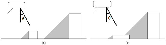 Figure 9. Double scatterers with smaller altitude distances are more likely to occur in typical layover scenarios. These scenarios can include buildings with different heights in layover with the ground (a) or the situation where a higher building is in layover with the ground and the roof of a lower building (b).
 - A higher building in layover with the roof and the ground of a smaller building: As depicted in Figure 9b, when a higher building is in layover with the roof and the ground of a smaller building, similar to the first scenario, it also leads to smaller elevation differences in the layover areas.
In both scenarios described, it is evident that scatterer pairs with smaller altitude distances are more likely to occur compared to those with larger distances. Assuming that the layover phenomenon is primarily initiated by the case depicted in Figure 9a, the probability density function of the altitude distance between two scatterers can be expressed as follows:
where is the probability density function of the building height, while gives the conditional distribution for given .
Under the assumption of homogeneous scattering properties for both the ground and the front wall, for a given value of (elevation difference), it is reasonable to accept that (elevation distance between two scatterers) follows a uniform distribution. This means that all possible values of within a certain range are equally likely.
Top of Form
Bottom of Form
where is the incidence angle (see Figure 9). Combining Equations (29) and (28), it yields
Two cases for height distributions are given below:
- Uniformly distributed building height: In the case that the heights of the buildings follow a uniform distribution ranging from zero to the maximum building height , i.e.,
- Discrete building height distribution: Really, due to city planning strategies, building heights often take on only a few discrete values.
Indeed, it is clear that many layover areas in urban environments consist of double scatterers with small elevation differences. Considering the limited altitude resolution produced by the restricted orbits of contemporary SAR sensors, achieving super-resolution is an indispensable requirement for high-quality tomographic SAR inversion in urban infrastructure monitoring.
In conclusion, elevation super-resolution is of paramount importance for tomographic SAR inversion for surveillance of urban infrastructure. The prevalence of scatterer pairs with small altitude differences highlights the necessity for achieving super-resolution. The significant increase in layover separation capability, nearly doubling it, is primarily attributed to the super-resolution capabilities of SL1MMER.
8.2. Urban Tomographic Imaging from PolSAR Data [72]
A complementary method for surveillance of urban infrastructure using SAR tomography expands upon the traditional two-dimensional SAR imaging concept by incorporating a third dimension, elevation. This is achieved by creating an additional synthetic aperture in elevation through a series of multi-baseline interferometric images. The result is a comprehensive 3-D representation of the scene’s reflectivity outline, encompassing azimuth, range, and altitude dimensions. TomoSAR methods enable the recognition of multiple scatterers within the same range-azimuth resolution cell [132]. Tomographic analysis can be carried out using various methods, including Fourier-based approaches, beamforming, or spectral analysis.
Distinguishing between reliable scatterers and false alarms presents a significant challenge in SAR tomography. The elevation sampling in the tomographic synthetic aperture is sparse and not as regular and dense as required by Fourier-based methods. This can lead to ambiguities and masking issues caused by anomalous sidelobes, along with the occurrence of noise, resulting in false alarms. In a study referenced as [133], this problem was tackled using a generalized likelihood ratio test (GLRT). The GLRT enables the assessment of detection success in terms of the probability of detecting scatterers while maintaining a fixed probability of false alarms. This statistical test relies on nonlinear maximization to detect single and double scatterers with a given probability of false alarms. The height of the detected scatterers is then assessed based on their positions within the unknown vector. One challenge to consider is that the GLRT detector’s performance tends to degrade when the number of measurements or scatterer coherence decreases [134]. To increase the number of acquisitions while maintaining high scatterer coherence, polarimetric systems can be leveraged. In recent work on PolSAR tomography over city regions [135], various spectral estimation methods were given to multi-pass SAR data obtained with changed polarization channels. This research focused on building layover scenarios and compared single and full polarization beamforming, Capon, and MUSIC techniques.
Figure 10 illustrates the multi-pass SAR interpretation in the range-elevation plane within a standard city environment. Three distinct contributions from the backscattered signal are emphasized, and these contributions all originate at the same distance from the platform. Consequently, they will intersect and interact within the same range-azimuth cell. In this context, it is important to note that the azimuth axis is positioned perpendicular to the plane. These three distinctive contributions stem from different parts of the scene, namely the ground, the building’s facade, and its roof. Within this specific scenario, the elevation profile of the backscattered reflectivity, referred to as will display solely three data points that deviate from zero. Top of Form
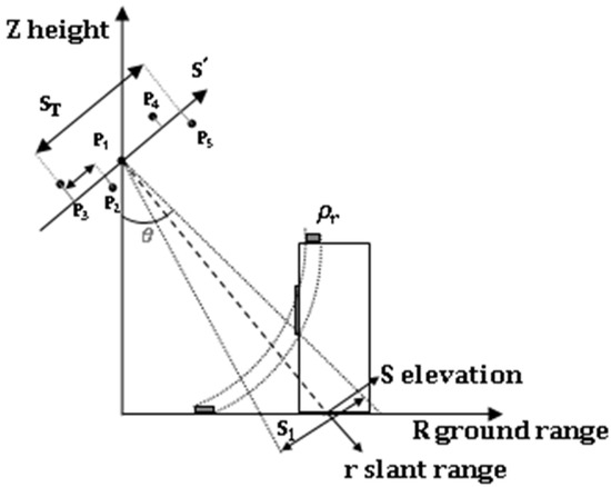
Figure 10.
A representation of the multi-pass SAR arrangement in the plane range–elevation ().
Bottom of Form
Furthermore, it is reasonable to assume that is sparse, with at maximum samples are not zero, normally with equal to 2. To assess the reflectivity function , a stack of M range-azimuth-focused images is assembled. The single-channel image, acquired along the orbit with the orthogonal baseline (as shown in Figure 10), at a fixed pixel, represents the process, which entails summing up the contributions from every scatterer positioned within the given range-azimuth resolution cell, with each scatterer situated at varying elevation coordinates . To obtain a discrete evaluation of , one would ideally discretize the integral operator.
We can represent the column vector containing the data on reflectivity at a fixed range and azimuth distance as . Therefore, the sampled data obtained can be expressed in relation to as follows:
In this context, is an observations column vector, represents an column vector associated with noise and clutter, and is an acquisition matrix that relates to the acquisition geometry. The generic element of this matrix, indexed by , can be expressed as follows:
with the operating wavelength, and the distance between the antenna position and the center of the scene. In the signal model described by Equation (33), several assumptions have been made, including the nonexistence of phase regulation, taking into consideration the atmospheric delay, and the non-existence of temporal and thermal distortions.
For fully polarimetric data, the received signal can be denoted as a observation column vector , with one vector for each polarimetric channel . Similarly, the reflectivity vector is 3N × 1, and it is assumed that all three polarimetric channels participate with the same sparse support, representing backscatter from the same structure within a range-azimuth cell 135. Under these assumptions, the signal model described by Equation (33) can be extended to the fully polarimetric case as follows:
where is a column vector corresponding to noise and clutter, and is a block diagonal measurement matrix, which is linked to the acquisition geometry, having the form:
where is an all-zero matrix.
Please note that model Equation (35) can be clearly adapted to the dual-polarization case by assuming only the two existing channels in the description of the vectors and , as well as two of the three blocks on the diagonal of , as expressed in Equation (36). TomoSAR techniques aim to estimate by inverting model Equation (35). However, this inversion is ill-posed because the acquisitions are not equally spaced, and generally , where is the number of polarization channels. Consequently, false alarms can occur in the rebuilt profiles, seriously modifying the accuracy of the results. The polarimetric reflectivity profile is assessed in this work using a GLRT (Generalized Likelihood Ratio Test) method. Supposing that is the maximum number of scatterers in each pixel, the vector is considered sparse, with at most significant samples. The detection problem can then be expressed in terms of the next statistical hypotheses:
Supposing a typical value of for the urban environment, w can be regarded as a circularly symmetric complex Gaussian noise vector. Therefore, when supposing deterministic scatterers, the vector u follows a circularly symmetric Gaussian distribution. At each step i, the following binary test is applied:
Top of Form
Bottom of Form
where is the expected support of cardinality of separate polarimetric vectors . Furthermore , supposed to be -sparse, with the matrix taken by replacing in Equation (36) the matrix in the place of , where is found from by extracting the columns of index . Furthermore, represents the anticipated support of cardinality for . The estimation of each support involves sequentially minimizing the term over supports of cardinality one. The thresholds for these tests can be determined through Monte Carlo simulations to achieve the desired probabilities of false alarm and false detection, denoted as , respectively, assuming .
In conclusion, this analysis extends the Fast-Sup-GLRT tomographic processing to the polarimetric case. Specifically, it demonstrates that the two-band polarization (HH + VV) approach can perform better than the single polarization (HH), even when the number of images is kept constant and a lower number of baselines is considered. The dual polarization approach gains an advantage over the single polarization approach by leveraging polarization diversity to compensate for the reduced baseline diversity. With two images acquired simultaneously with different polarizations for each baseline, this approach can be effective, especially when there is no ground alternation with time.
Concluding this section, it is essential to recognize that new methods with various characteristics appear constantly, giving rise to very detailed representations of tomographic urban representations [136,137,138]. Accordingly, Rambour et al. proposed [136] a method for urban surface reconstruction in SAR tomography by graph cuts. On the other hand, Huang and Ferro-Famil introduced [137] a way to characterize 3-D urban areas using high-resolution polarimetric SAR tomographic techniques and a minimal number of acquisitions. Finally, Shi et al. proposed [138] the generation of large-scale high-quality 3-D urban models.
9. Conclusions
Monitoring the development of urban regions is essential for environmental reasons and the organized development of cities. A powerful tool for this purpose is the SAR data available from SAR sensors onboard various satellites. In this review paper, we had the opportunity to revisit important works, which were categorized according to their content as follows:
- SAR features that are prominent for use in urban area classification.
- Classification techniques that are usually employed.
- Ways of fusing SAR images with other data for improving urban area categorization.
- Use of decorrelation and interferometric properties to detect changes in urban areas.
- Use of SAR data in the construction of tomographic and DEM models.
Some of the recent works contain a combination of the above topics, making the entire discipline of urban planning with SAR data very attractive. The material exposed so far from Section 2 up to Section 9 constitutes indicative research methods for the extent and depth of the field.
In summarizing the results of the presented works, it is important to stay with the most interesting concepts. The study presented in [2] demonstrated that the characterization of an urban environment can be significantly enhanced by employing multiscale textural features extracted from satellite SAR data. In summary, both the MIM and MRMR methods, which facilitate the ranking and selection of a minimal subset from an extensive set of ICTD parameters, demonstrate their effectiveness in achieving precise image classification. In order to investigate the performance of classifying land cover types under various percentages of cloud content, the study in Section 3 required datasets with different cloud contents. Quantitative metrics, including the standard accuracy metrics of the overall accuracy, the confusion matrix, the producer’s accuracy, and the user’s accuracy, were employed to evaluate the results. Unaffected surfaces were created in Section 4 by combining formerly assessed unaffected surfaces obtained from separate image sources using the Dempster–Shafer fusion rules. Evaluation of the accuracy revealed that unaffected surfaces from urban regions derived from visual data achieved an improved classification performance of 89.68% compared to those derived from SAR data, which achieved a classification accuracy of 68.80%. When additional spectral and texture features were incorporated, the overall classification accuracy further improved to 95.33%. The work [55] described in Section 6 presents a technique for mapping floods in city areas using SAR intensity and interferometric coherence within the Bayesian network fusion framework. It combines intensity and coherence data probabilistically and accounts for flood uncertainty related to both intensity and coherence. This approach effectively gets flood information across diverse types of land cover and provides maps indicating both the coverage and type of flooding. In the context of embankment detection in Section 7, the primary focus was on the area flooded by river water. To achieve this, the water resulting from ponding was excluded. This process involved removing ponding water from the initial binary water map, resulting in what we term a “fluvial flood map.” In Section 8, the analysis extends the Fast-Sup-GLRT tomographic processing to the polarimetric case. Specifically, it demonstrates that the two-band polarization (HH + VV) approach can perform better than the single polarization (HH), even when the number of images is kept constant and a lower number of baselines is considered. The dual polarization approach gains an advantage over the single polarization approach by leveraging polarization diversity to compensate for the reduced baseline diversity.
Recent advancements in synthetic aperture radar (SAR) technology have led to exciting new trends [139,140] in its use for urban planning. Notably:
Multi-Temporal SAR Analysis: There is a growing trend towards the use of multi-temporal SAR data for urban planning. By analyzing SAR images acquired over different time periods, urban planners can monitor urban growth, track changes in land use, and assess the impact of urban development projects over time.
Integration with Other Remote Sensing Data: SAR data is being integrated with other remote sensing datasets, such as LiDAR and optical imagery, to provide comprehensive insights into urban environments. By combining SAR data with data from other sources, urban planners can gain a more holistic understanding of urban landscapes and make informed decisions.
Machine Learning and AI for SAR Image Analysis: Machine learning and artificial intelligence techniques are being applied to SAR image analysis, enabling automated feature extraction, classification, and change detection in urban areas. These advanced algorithms enhance the efficiency and accuracy of urban planning processes by automating time-consuming tasks and providing actionable insights from SAR data.
SAR Data Sharing and Open Access Initiatives: There is a growing emphasis on SAR data sharing and open access initiatives, which aim to make SAR data more accessible to urban planners, researchers, and decision-makers. Open SAR data repositories and platforms facilitate the dissemination and use of SAR data for urban planning applications, fostering collaboration and innovation in the field.
Overall, these emerging trends demonstrate the increasing importance of SAR technology in urban planning and highlight its potential to address key challenges in sustainable urban development and management.
Recent publications showcase the ongoing advancements in SAR technology and methodologies, particularly in SAR tomography, elevation modeling, and the integration of deep learning techniques for improved analysis of SAR data [141,142,143,144,145,146].
Funding
This research received no external funding.
Data Availability Statement
The data are available upon request.
Conflicts of Interest
The author declares no conflicts of interest.
References
- Negri, M.; Gamba, P.; Lisini, G.; Tupin, F. Junction-aware extraction and regularization of urban road networks in high-resolution SAR images. IEEE Trans. Geosci. Remote Sens. 2006, 44, 2962–2971. [Google Scholar] [CrossRef]
- Dell’Acqua, F.; Gamba, P. Discriminating urban environments using multiscale texture and multiple SAR images. Int. J. Remote Sens. 2006, 27, 3797–3812. [Google Scholar] [CrossRef]
- Perissin, D.; Ferretti, A. Urban-Target Recognition by Means of Repeated Spaceborne SAR Images. IEEE Trans. Geosci. Remote Sens. 2007, 45, 4043–4058. [Google Scholar] [CrossRef]
- Ainsworth, T.L.; Schuler, D.L.; Lee, J.S. Polarimetric SAR characterization of man-made structures in urban areas using normalized circular-pol correlation coefficients. Remote Sens. Environ. 2008, 112, 2876–2885. [Google Scholar] [CrossRef]
- Gamba, P.; Aldrighi, M.; Stasolla, M. Robust Extraction of Urban Area Extents in HR and VHR SAR Images. IEEE J. Sel. Top. Appl. Earth Obs. Remote Sens. 2011, 4, 27–34. [Google Scholar] [CrossRef]
- Ban, Y.; Yousif, O.A. Multitemporal Spaceborne SAR Data for Urban Change Detection in China. IEEE J. Sel. Top. Appl. Earth Obs. Remote Sens. 2012, 5, 1087–1094. [Google Scholar] [CrossRef]
- Yousif, O.; Ban, Y. Improving Urban Change Detection From Multitemporal SAR Images Using PCA-NLM. IEEE Trans. Geosci. Remote Sens. 2013, 51, 2032–2041. [Google Scholar] [CrossRef]
- Siu, L.W.; Hart, M.A. Quantifying urban heat island intensity in Hong Kong SAR, China. Environ. Monit. Assess. 2013, 185, 4383–4398. [Google Scholar] [CrossRef] [PubMed]
- Ban, Y.; Jacob, A.; Gamba, P. Spaceborne SAR data for global urban mapping at 30 m resolution using a robust urban extractor. ISPRS J. Photogramm. Remote Sens. 2015, 103, 28–37. [Google Scholar] [CrossRef]
- Bhattacharya, A.; Touzi, R. Polarimetric SAR urban classification using the Touzi target scattering decomposition. Can. J. Remote Sens. 2011, 37, 323332. [Google Scholar] [CrossRef]
- Fusilli, L.; Marzialetti, P.; Laneve, G.; Santilli, G. Urban growth assessment around Winam Gulf of Kenya based on satellite imagery. Acta Astronaut. 2014, 93, 279–290. [Google Scholar] [CrossRef]
- Plyer, A.; Colin-Koeniguer, E.; Weissgerber, F. A New Coregistration Algorithm for Recent Applications on Urban SAR Images. IEEE Geosci. Remote Sens. Lett. 2015, 12, 2198–2202. [Google Scholar] [CrossRef]
- Poursanidis, D.; Chrysoulakis, N.; Mitraka, Z. Landsat 8 vs. Landsat 5: A comparison based on urban and peri-urban land cover mapping. Int. J. Appl. Earth Obs. Geoinf. 2015, 35 Pt B, 259–269. [Google Scholar] [CrossRef]
- Xiang, D.; Ban, Y.; Su, Y. Model-Based Decomposition with Cross Scattering for Polarimetric SAR Urban Areas. IEEE Geosci. Remote Sens. Lett. 2015, 12, 2496–2500. [Google Scholar] [CrossRef]
- Azmedroub, B.; Ouarzeddine, M.; Souissi, B. Extraction of Urban Areas From Polarimetric SAR Imagery. IEEE J. Sel. Top. Appl. Earth Obs. Remote Sens. 2016, 9, 2583–2591. [Google Scholar] [CrossRef]
- Kafy, A.-A.; Faisal, A.-A.; Shuvo, R.M.; Naim, N.H.; Sikdar, S.; Chowdhury, R.R.; Islam, A.; Sarker, H.S.; Khan, H.H.; Kona, M.A. Remote sensing approach to simulate the land use/land cover and seasonal land surface temperature change using machine learning algorithms in a fastest-growing megacity of Bangladesh. Remote Sens. Appl. Soc. Environ. 2021, 21, 100463. [Google Scholar] [CrossRef]
- Otukei, J.R.; Blaschke, T. Land cover change assessment using decision trees, support vector machines and maximum likelihood classification algorithms. Int. J. Appl. Earth Obs. Geoinf. 2010, 12, S27–S31. [Google Scholar] [CrossRef]
- Hu, H.; Ban, Y. Unsupervised Change Detection in Multitemporal SAR Images Over Large Urban Areas. IEEE J. Sel. Top. Appl. Earth Obs. Remote Sens. 2014, 7, 3248–3261. [Google Scholar] [CrossRef]
- Lv, Q.; Dou, Y.; Niu, X.; Xu, J.; Xu, J.; Xia, F. Urban Land Use and Land Cover Classification Using Remotely Sensed SAR Data through Deep Belief Networks. J. Sens. 2015, 2015, 538063. [Google Scholar] [CrossRef]
- Zhang, H.; Lin, H.; Li, Y.; Zhang, Y.; Fang, C. Mapping urban impervious surface with dual-polarimetric SAR data: An improved method. Landsc. Urban Plan. 2016, 151, 55–63. [Google Scholar] [CrossRef]
- Xiang, D.; Tang, T.; Ban, Y.; Su, Y.; Kuang, G. Unsupervised polarimetric SAR urban area classification based on model-based decomposition with cross scattering. ISPRS J. Photogramm. Remote Sens. 2016, 116, 86–100. [Google Scholar] [CrossRef]
- Zhang, H.; Lin, H.; Wang, Y. A new scheme for urban impervious surface classification from SAR Images. ISPRS J. Photogramm. Remote Sens. 2018, 139, 103–118. [Google Scholar] [CrossRef]
- Audebert, N.; Le Saux, B.; Lefèvre, S. Beyond RGB: Very high resolution urban remote sensing with multimodal deep networks. ISPRS J. Photogramm. Remote Sens. 2018, 140, 20–32. [Google Scholar] [CrossRef]
- Huang, B.; Zhao, B.; Song, Y. Urban land-use mapping using a deep convolutional neural network with high spatial resolution multispectral remote sensing imagery. Remote Sens. Environ. 2018, 214, 73–86. [Google Scholar] [CrossRef]
- Zhang, C.; Sargent, I.; Pan, X.; Li, H.; Gardiner, A.; Hare, J.; Atkinson, P.M. Joint Deep Learning for land cover and land use classification. Remote Sens. Environ. 2019, 221, 173–187. [Google Scholar] [CrossRef]
- Heydari, S.S.; Mountrakis, G. Meta-analysis of deep neural networks in remote sensing: A comparative study of mono-temporal classification to support vector machines. ISPRS J. Photogramm. Remote Sens. 2019, 152, 192–210. [Google Scholar] [CrossRef]
- Wang, X.; Cavigelli, L.; Eggimann, M.; Magno, M.; Benini, L. HR-SAR-Net: A Deep Neural Network for Urban Scene Segmentation from High-Resolution SAR Data. In Proceedings of the 2020 IEEE Sensors Applications Symposium (SAS), Kuala Lumpur, Malaysia, 9–11 March 2020. [Google Scholar] [CrossRef]
- Ling, J.; Zhang, H.; Lin, Y. Improving Urban Land Cover Classification in Cloud-Prone Areas with Polarimetric SAR Images. Remote Sens. 2021, 13, 4708. [Google Scholar] [CrossRef]
- Prasad, P.; Loveson, V.J.; Chandra, P.; Kotha, M. Evaluation and comparison of the earth observing sensors in land cover/land use studies using machine learning algorithms. Ecol. Inform. 2022, 68, 101522. [Google Scholar] [CrossRef]
- Garzelli, A. Wavelet-Based Fusion of Optical and SAR Image Data over Urban area. In Proceedings of the International Archives of the Photogrammetry, Remote Sensing and Spatial Information Sciences, Melbourne, Australia, 25 August–1 September 2002; Available online: https://citeseerx.ist.psu.edu/document?repid=rep1&type=pdf&doi=5a43905748226bcbf0bc24598d58dfb872e7d4c6 (accessed on 20 August 2023).
- Gomez-Chova, L.; Fernández-Prieto, D.; Calpe, J.; Soria, E.; Vila, J.; Camps-Valls, G. Urban monitoring using multi-temporal SAR and multi-spectral data. Pattern Recognit. Lett. 2006, 27, 234–243. [Google Scholar] [CrossRef]
- Gamba, P.; Dell’Acqua, F.; Lisini, G. Change Detection of Multitemporal SAR Data in Urban Areas Combining Feature-Based and Pixel-Based Techniques. IEEE Trans. Geosci. Remote Sens. 2006, 44, 2820–2827. [Google Scholar] [CrossRef]
- Brenner, A.R.; Roessing, L. Radar Imaging of Urban Areas by Means of Very High-Resolution SAR and Interferometric SAR. IEEE Trans. Geosci. Remote Sens. 2008, 46, 2971–2982. [Google Scholar] [CrossRef]
- Corbane, C.; Faure, J.-F.; Baghdadi, N.; Villeneuve, N.; Petit, M. Rapid Urban Mapping Using SAR/Optical Imagery Synergy. Sensors 2008, 8, 7125–7143. [Google Scholar] [CrossRef] [PubMed]
- Pacifici, F.; Del Frate, F.; Emery, W.J.; Gamba, P.; Chanussot, J. Urban Mapping Using Coarse SAR and Optical Data: Outcome of the 2007 GRSS Data Fusion Contest. IEEE Geosci. Remote Sens. 2008, 5, 331–335. [Google Scholar] [CrossRef]
- Amarsaikhana, D.; Blotevogelb, H.H.; Van Genderenc, J.L.; Ganzoriga, M.; Gantuyaaand, R.; Nergui, B. Fusing high-resolution SAR and optical imagery for improved urban land cover study and classification. Int. J. Image Data Fusion 2010, 1, 83–97. [Google Scholar] [CrossRef]
- Ban, Y.; Hu, H.; Rangel, I.M. Fusion of Quickbird MS and RADARSAT SAR data for urban landcover mapping: Object-based and knowledge-based approach. Int. J. Remote Sens. 2010, 31, 1391–1410. [Google Scholar] [CrossRef]
- Zhu, Z.; Woodcock, C.E.; Rogan, J.; Kellndorfer, J. Assessment of spectral, polarimetric, temporal, and spatial dimensions for urban and peri-urban land cover classification using Landsat and SAR data. Remote Sens. Environ. 2012, 117, 72–82. [Google Scholar] [CrossRef]
- Gamba, P.; Aldrighi, M. SAR Data Classification of Urban Areas by Means of Segmentation Techniques and Ancillary Optical Data. IEEE J. Sel. Top. Appl. Earth Obs. Remote Sens. 2012, 5, 140–1148. [Google Scholar] [CrossRef]
- Shao, Z.; Fu, H.; Fu, P.; Yin, L. Mapping Urban Impervious Surface by Fusing Optical and SAR Data at the Decision Level. Remote Sens. 2016, 8, 945. [Google Scholar] [CrossRef]
- Mou, L.; Schmitt, M.; Wang, Y.; Zhu, X.X. A CNN for the identification of corresponding patches in SAR and optical imagery of urban scenes. In Proceedings of the 2017 Joint Urban Remote Sensing Event (JURSE), Dubai, United Arab Emirates, 4–7 March 2017. [Google Scholar] [CrossRef]
- Zhang, L.; Weng, Q.; Shao, Z. An evaluation of monthly impervious surface dynamics by fusing Landsat and MODIS time series in the Pearl River Delta, China, from 2000 to 2015. Remote Sens. Environ. 2017, 201, 99–114. [Google Scholar] [CrossRef]
- Zhou, T.; Pan, J.; Zhang, P.; Wei, S.; Han, T. Mapping Winter Wheat with Multi-Temporal SAR and Optical Images in an Urban Agricultural Region. Sensors 2017, 17, 1210. [Google Scholar] [CrossRef]
- Haas, J.; Ban, Y. Sentinel-1A SAR and sentinel-2A MSI data fusion for urban ecosystem service mapping. Remote Sens. Appl. Soc. Environ. 2017, 8, 41–53. [Google Scholar] [CrossRef]
- Zhang, H.; Xu, R. Exploring the optimal integration levels between SAR and optical data for better urban land cover mapping in the Pearl River Delta. Int. J. Appl. Earth Obs. Geoinf. 2018, 64, 87–95. [Google Scholar] [CrossRef]
- Zhang, H.; Li, J.; Wang, T.; Lin, H.; Zheng, Z.; Li, Y.; Lu, Y. A manifold learning approach to urban land cover classification with optical and radar data. Landsc. Urban Plan. 2018, 172, 11–24. [Google Scholar] [CrossRef]
- Yonezawa, C.; Takeuchi, S. Decorrelation of SAR data by urban damages caused by the 1995 Hyogoken-nanbu earthquake. Int. J. Remote Sens. 2001, 22, 1585–1600. [Google Scholar] [CrossRef]
- Mingsheng, L.; Liming, J.; Hui, L.; Bo, H.; Jianya, G. Urban Change Detection Based on Coherence and Intensity Characteristics of SAR Imagery. ISPRS J. Photogramm. Remote Sens. 2008, 8, 999–1006. [Google Scholar] [CrossRef]
- Chen, S.W.; Wang, X.S.; Xiao, S.P. Urban Damage Level Mapping Based on Co-Polarization Coherence Pattern Using Multitemporal Polarimetric SAR Data. IEEE J. Sel. Top. Appl. Earth Obs. Remote Sens. 2018, 11, 2657–2667. [Google Scholar] [CrossRef]
- Manzoni, M.; Monti-Guarnieri, A.; Molinari, M.E. Joint exploitation of spaceborne SAR images and GIS techniques for urban coherent change detection. Remote Sens. Environ. 2021, 253, 112152. [Google Scholar] [CrossRef]
- Gernhardta, S.; Adamb, N.; Einederband, M.; Bamler, R. Potential of very high resolution SAR for persistent scatterer interferometry in urban areas. Ann. GIS 2010, 16, 103–111. [Google Scholar] [CrossRef]
- Wang, Y.; Zhu, X.X.; Bamler, R. Retrieval of phase history parameters from distributed scatterers in urban areas using very high resolution SAR data. ISPRS J. Photogramm. Remote Sens. 2012, 73, 89–99. [Google Scholar] [CrossRef]
- Pulvirenti, L.; Chini, M.; Pierdicca, N.; Boni, G. Use of SAR Data for Detecting Floodwater in Urban and Agricultural Areas: The Role of the Interferometric Coherence. IEEE Trans. Geosci. Remote Sens. 2016, 54, 1532–1544. [Google Scholar] [CrossRef]
- Sica, F.; Pulella, A.; Nannini, M.; Pinheiro, M.; Rizzoli, P. Repeat-pass SAR interferometry for land cover classification: A methodology using Sentinel-1 Short-Time-Series. Remote Sens. Environ. 2019, 232, 111277. [Google Scholar] [CrossRef]
- Li, Y.; Martinis, S.; Wieland, M.; Schlaffer, S.; Natsuaki, R. Urban Flood Mapping Using SAR Intensity and Interferometric Coherence via Bayesian Network Fusion. Remote Sens. 2019, 11, 2231. [Google Scholar] [CrossRef]
- Schumann, G.J.-P.; Neal, J.C.; Mason, D.C.; Bates, P.D. The accuracy of sequential aerial photography and SAR data for observing urban flood dynamics, a case study of the UK summer 2007 floods. Remote Sens. Environ. 2011, 115, 2536–2546. [Google Scholar] [CrossRef]
- Meesuk, V.; Vojinovic, Z.; Mynett, A.E.; Abdullah, A.F. Urban flood modelling combining top-view LiDAR data with ground-view SfM observations. Adv. Water Resour. 2015, 75, 105–117. [Google Scholar] [CrossRef]
- Wood, M.; De Jong, S.M.; Straatsma, M.W. Locating flood embankments using SAR time series: A proof of concept International. Int. J. Appl. Earth Obs. Geoinf. 2018, 70, 72–83. [Google Scholar] [CrossRef]
- Dasgupta, A.; Grimaldi, S.; Ramsankaran, R.A.A.J.; Pauwels, V.R.N.; Walker, J.P. Towards operational SAR-based flood mapping using neuro-fuzzy texture based approaches. Remote Sens. Environ. 2018, 215, 313–329. [Google Scholar] [CrossRef]
- Rambour, C.; Budillon, A.; Johnsy, A.C.; Denis, L.; Tupin, F.; Schirinzi, G. From Interferometric to Tomographic SAR: A Review of Synthetic Aperture Radar Tomography-Processing Techniques for Scatterer Unmixing in Urban Areas. IEEE Geosci. Remote Sens. Mag. 2020, 8, 6–29. [Google Scholar] [CrossRef]
- Oriot, H.; Cantalloube, H. Circular SAR imagery for urban remote sensing. In Proceedings of the 7th European Conference on Synthetic Aperture Radar, Friedrichshafen, Germany, 2–5 June 2008. [Google Scholar]
- Fornaro, G.; Serafino, F. Imaging of Single and Double Scatterers in Urban Areas via SAR Tomography. IEEE Trans. Geosci. Remote Sens. 2006, 44, 3497–3505. [Google Scholar] [CrossRef]
- Zhu, X.X.; Bamler, R. Very High Resolution Spaceborne SAR Tomography in Urban Environment. IEEE Trans. Geosci. Remote Sens. 2010, 48, 4296–4308. [Google Scholar] [CrossRef]
- Sportouche, H.; Tupin, F.; Denise, L. Extraction and Three-Dimensional Reconstruction of Isolated Buildings in Urban Scenes From High-Resolution Optical and SAR Spaceborne Images. IEEE Geosci. Remote Sens. 2011, 49, 3932–3946. [Google Scholar] [CrossRef]
- Zhu, X.X.; Bamler, R. Demonstration of Super-Resolution for Tomographic SAR Imaging in Urban Environment. IEEE Trans. Geosci. Remote Sens. 2012, 50, 3150–3157. [Google Scholar] [CrossRef]
- Palm, S.; Oriot, H.M.; Cantalloube, H.M. Radargrammetric DEM Extraction Over Urban Area Using Circular SAR Imagery. IEEE Trans. Geosci. Remote Sens. 2012, 50, 4720–4725. [Google Scholar] [CrossRef]
- Zhu, X.X.; Bamler, R. Superresolving SAR Tomography for Multidimensional Imaging of Urban Areas: Compressive sensing-based TomoSAR inversion. IEEE Signal Process. Mag. 2014, 31, 51–58. [Google Scholar] [CrossRef]
- Zhu, X.X.; Ge, N.; Shahzad, M. Joint Sparsity in SAR Tomography for Urban Mapping. IEEE J. Sel. Top. 2015, 9, 1498–1509. [Google Scholar] [CrossRef]
- Bagheri, H.; Schmitt, M.; d’Angelo, P.; Zhu, X.X. A framework for SAR-optical stereogrammetry over urban areas. ISPRS J. Photogramm. Remote Sens. 2018, 146, 389–408. [Google Scholar] [CrossRef]
- Wu, B.; Xie, L.; Hu, H.; Zhu, Q.; Yau, E. Integration of aerial oblique imagery and terrestrial imagery for optimized 3D modeling in urban areas. ISPRS J. Photogramm. Remote Sens. 2018, 139, 119–132. [Google Scholar] [CrossRef]
- Hou, Y.; Peng, J.; Hu, Z.; Tao, P.; Shan, J. Planarity constrained multi-view depth map reconstruction for urban Scenes. ISPRS J. Photogramm. Remote Sens. 2018, 139, 133–145. [Google Scholar] [CrossRef]
- Budillon, A.; Johnsy, A.C.; Schirinzi, G. Urban Tomographic Imaging Using Polarimetric SAR Data. Remote Sens. 2019, 11, 132. [Google Scholar] [CrossRef]
- Tebaldini, S.; Manzoni, M.; Tagliaferri, D.; Rizzi, M.; Monti-Guarnieri, A.V.; Prati, C.M.; Spagnolini, U.; Nicoli, M.; Russo, I.; Mazzucco, C. Sensing the Urban Environment by Automotive SAR Imaging: Potentials and Challenges. Remote Sens. 2022, 14, 3602. [Google Scholar] [CrossRef]
- Dong, H.; Zhang, L.; Zou, B. Exploring Vision Transformers for Polarimetric SAR Image Classification. IEEE Trans. Geosci. Remote Sens. 2022, 60, 5219715. [Google Scholar] [CrossRef]
- Pang, L.; Sun, J.; Chi, Y.; Yang, Y.; Zhang, F.; Zhang, L. CD-TransUNet: A Hybrid Transformer Network for the Change Detection of Urban Buildings Using L-Band SAR Images. Sustainability 2022, 14, 9847. [Google Scholar] [CrossRef]
- Li, L.; Wang, C.; Zhang, H.; Zhang, K. SAR Image Urban Scene Classification based on an Optimized Conditional Generative Adversarial Network. In Proceedings of the 2019 SAR in Big Data Era (BIGSARDATA), Beijing, China, 5–6 May 2019; pp. 1–4. [Google Scholar] [CrossRef]
- Yang, Q.; Shen, X.; Zhang, Q.; Helfrich, S.; Kellndorfer, J.M.; Hao, W. Promoting SAR-Based Urban Flood Mapping with Adversarial Generative Network and Out of Distribution Detection. In Proceedings of the IEEE International Geoscience and Remote Sensing Symposium, Pasadena, CA, USA, 16–21 July 2023; pp. 2336–2338. [Google Scholar] [CrossRef]
- Huang, H.; Lei, X.; Liao, W.; Zuo, X.; Wang, H. A novel multi-strategy hydrological feature extraction (MHFE) method to improve urban waterlogging risk prediction, a case study of Fuzhou City in China. Sci. Total Environ. 2023, 904, 165834. [Google Scholar] [CrossRef] [PubMed]
- Della’Acqua, F.; Gamba, P. Texture-based characterization of urban environments on satellite SAR images. IEEE Trans. Geosci. Remote Sens. 2003, 41, 153–159. [Google Scholar] [CrossRef]
- Karachristos, K.; Koukiou, G.; Anastassopoulos, V. PolSAR Cell Information Representation by a Pair of Elementary Scatterers. Remote Sens. 2022, 14, 695. [Google Scholar] [CrossRef]
- Li, L.; Gao, J.; Ge, H.; Zhang, Y.; ·Haifei Zhang, H. An effective feature extraction method via spectral-spatial filter discrimination analysis for hyperspectral image. Multimed. Tools Appl. 2022, 81, 40871–40904. [Google Scholar] [CrossRef]
- Cloude, S.R.; Pottier, E. A review of target decomposition theorems in radar polarimetry. IEEE Trans. Geosci. Remote Sens. 1996, 34, 498518. [Google Scholar] [CrossRef]
- Touzi, R. Target scattering decomposition in terms of roll-inavriant target parameters. IEEE Trans. Geosci. Remote Sens. 2007, 45, 7384. [Google Scholar] [CrossRef]
- Shannon, C. A mathematical theory of communication. Bell Syst. Tech. J. 1948, 27, 379–423. [Google Scholar] [CrossRef]
- Fano, R. Transmission of Information: Statistical Theory of Communications, 3rd ed.; Wiley: New York, NY, USA, 1961; pp. 1–389. [Google Scholar]
- Hellman, M.E.; Raviv, J. Probability of error, equivocation, and the Chernoff bound. IEEE Trans. Inf. Theory 1970, 16, 368372. [Google Scholar] [CrossRef]
- King, M.D.; Platnick, S.; Menzel, W.P.; Ackerman, S.A.; Hubanks, P.A. Spatial and temporal distribution of clouds observed by MODIS onboard the Terra and Aqua satellites. IEEE Trans. Geosci. Remote Sens. 2013, 51, 3826–3852. [Google Scholar] [CrossRef]
- Zhang, Y.; Zhang, H.; Lin, H. Improving the impervious surface estimation with combined use of optical and SAR remote sensing images. Remote Sens. Environ. 2014, 141, 155–167. [Google Scholar] [CrossRef]
- Chen, W.; Hai, D.; Gou, S.; Jiao, L. Classification on PolSAR images based on SVM with Self-Paced Learning optimization. In Proceedings of the 2018 IEEE International Geoscience and Remote Sensing Symposium, Valencia, Spain, 22–27 July 2018. [Google Scholar] [CrossRef]
- Hao, P.-Y.; Chiang, J.-H.; Chen, Y.-D. Possibilistic classification by support vector networks. J. Neural Netw. 2022, 149, 40–56. [Google Scholar] [CrossRef] [PubMed]
- Breiman, L. Random forests. Mach. Learn. 2001, 45, 5–32. [Google Scholar] [CrossRef]
- Diao, W.; Sun, X.; Zheng, X.; Dou, F.; Wang, H.; Fu, K. Efficient saliency-based object detection in remote sensing images using deep belief networks. IEEE Geosci. Remote Sens. Lett. 2016, 13, 137–141. [Google Scholar] [CrossRef]
- Clinton, N.; Yu, L.; Gong, P. Geographic stacking: Decision fusion to increase global land cover map accuracy. ISPRS J. Photogramm. Remote Sens. 2015, 103, 57–65. [Google Scholar] [CrossRef]
- Sun, Z.; Xu, R.; Du, W.; Wang, L.; Lu, D. High-resolution urban land mapping in China from sentinel 1A/2 imagery based on Google Earth Engine. Remote Sens. 2019, 11, 752. [Google Scholar] [CrossRef]
- Freeman, A.; Durden, S.L. A three-component scattering model for polarimetric SAR data. IEEE Trans. Geosci. Remote Sens. 1998, 36, 963–973. [Google Scholar] [CrossRef]
- Cloude, S.R.; Pottier, E. An entropy based classification scheme for land applications of polarimetric SAR. IEEE Trans. Geosci. Remote Sens. 1997, 35, 68–78. [Google Scholar] [CrossRef]
- Yamaguchi, Y.; Moriyama, T.; Ishido, M.; Yamada, H. Four-component scattering model for polarimetric SAR image decomposition. IEEE Trans. Geosci. Remote Sens. 2005, 43, 1699–1706. [Google Scholar] [CrossRef]
- Yu, X.; Hyyppä, J.; Vastaranta, M.; Holopainen, M.; Viitala, R. Predicting individual tree attributes from airborne laser point clouds based on the random forests technique. ISPRS J. Photogramm. Remote Sens. 2011, 66, 28–37. [Google Scholar] [CrossRef]
- Szegedy, C.; Liu, W.; Jia, Y.; Sermanet, P.; Reed, S.; Anguelov, D.; Erhan, D.; Vanhoucke, V.; Rabinovich, A. Going deeper with convolutions. In Proceedings of the IEEE Conference on Computer Vision and Pattern Recognition, Boston, MA, USA, 7–12 June 2015; pp. 1–9. [Google Scholar]
- Yang, L.; Huang, C.; Homer, C.G.; Wylie, B.K.; Coan, M.J.; Corporation, R.; Survey, G.; Data, E.; Falls, S.; Usgs, L.Y.; et al. An approach for mapping large-area impervious surfaces: Synergistic use of Landsat 7 ETM+ and high spatial resolution imagery. Can. J. Remote Sens. 2003, 29, 230–240. [Google Scholar] [CrossRef]
- Weng, Q.; Hu, X. Medium spatial resolution satellite imagery for estimating and mapping urban impervious surfaces using LSMA and ANN. IEEE Trans. Geosci. Remote Sens. 2008, 46, 2397–2406. [Google Scholar] [CrossRef]
- Zhang, L.; Weng, Q. Annual dynamics of impervious surface in the Pearl River Delta, China, from 1988 to 2013, using time series Landsat imagery. ISPRS J. Photogramm. Remote Sens. 2016, 113, 86–96. [Google Scholar] [CrossRef]
- Shao, Z.; Liu, C. The integrated use of DMSP-OLS nighttime light and MODIS data for monitoring large-scale impervious surface dynamics: A case study in the Yangtze River Delta. Remote Sens. 2014, 6, 9359–9378. [Google Scholar] [CrossRef]
- Weng, Q. Remote sensing of impervious surfaces in the urban areas: Requirements, methods, and trends. Remote Sens. Environ. 2012, 117, 34–49. [Google Scholar] [CrossRef]
- Zhang, J.; Yang, J.; Zhao, Z.; Li, H.; Zhang, Y. Block-regression based fusion of optical and SAR imagery for feature enhancement. Int. J. Remote Sens. 2010, 31, 2325–2345. [Google Scholar] [CrossRef]
- Dempster, A.P. Upper and lower probabilities induced by multivalue mapping. Ann. Math. Stat. 1967, 38, 325–339. [Google Scholar] [CrossRef]
- Shafer, G. A Mathematical Theory of Evidence; Princeton University Press: Princeton, NJ, USA, 1976. [Google Scholar]
- Ran, Y.; Li, X.; Lu, L.; Li, Z. Large-scale land cover mapping with the integration of multi-source information based on teh Dempster-Shafer theory. Int. J. Geogr. Inf. Sci. 2012, 26, 169–191. [Google Scholar] [CrossRef]
- Lu, L.; Xie, W.; Zhang, J.; Huang, G.; Li, Q.; Zhao, Z. Woodland extraction from high-resolution CASMSAR data based on dempster-shafer evidence theory fusion. Remote Sens. 2015, 7, 4068–4091. [Google Scholar] [CrossRef]
- Haralick, R.M.; Shanmugam, K.; Dinstein, I. Textural features for image classification. IEEE Trans. Syst. Man Cybern. 1973, 3, 610–621. [Google Scholar] [CrossRef]
- Ho, T.K. The random subspace method for constructing decision forests. IEEE Trans. Pattern Anal. Mach. Intell. 1998, 20, 832–844. [Google Scholar]
- Chen, S.-W.; Li, Y.-Z.; Wang, X.-S.; Xiao, S.-P.; Sato, M. Modeling and interpretation of scattering mechanisms in polarimetric synthetic aperture radar: Advances and perspectives. IEEE Signal Process. Mag. 2014, 31, 79–89. [Google Scholar] [CrossRef]
- Chen, S.-W.; Sato, M. Tsunami damage investigation of built-up areas using multitemporal spaceborne full polarimetric SAR images. IEEE Trans. Geosci. Remote Sens. 2013, 51, 1985–1997. [Google Scholar] [CrossRef]
- Touzi, R.; Lopes, A.; Bruniquel, J.; Vachon, P.W. Coherence estimation for SAR imagery. IEEE Trans. Geosci. Remote Sens. 1999, 37, 135–149. [Google Scholar] [CrossRef]
- Chen, S.-W.; Wang, X.-S.; Sato, M. Uniform polarimetric matrix rotation theory and its applications. IEEE Trans. Geosci. Remote Sens. 2014, 52, 4756–4770. [Google Scholar] [CrossRef]
- Chen, S.-W. Polarimetric coherence pattern: A visualization and characterization tool for PolSAR data investigation. IEEE Trans. Geosci. Remote Sens. 2018, 56, 286–297. [Google Scholar] [CrossRef]
- Sato, M.; Chen, S.-W.; Satake, M. Polarimetric SAR analysis of tsunami damage following the 11 March 2011 East Japan Earthquake. Proc. IEEE 2012, 100, 2861–2875. [Google Scholar] [CrossRef]
- Chen, S.-W.; Wang, X.-S.; Sato, M. PolInSAR complex coherence estimation based on covariance matrix similarity test. IEEE Trans. Geosci. Remote Sens. 2012, 50, 4699–4710. [Google Scholar] [CrossRef]
- Chini, M.; Pulvirenti, L.; Pierdicca, N. Analysis and interpretation of the COSMO-SkyMed observations of the 2011 Japan tsunami. IEEE Geosci. Remote Sens. Lett. 2012, 9, 467–471. [Google Scholar] [CrossRef]
- Zebker, H.A.; Member, S.; Villasenor, J. Decorrelation in Interferometric Radar Echoes. IEEE Trans. Geosci. Remote Sens. 1992, 30, 950–959. [Google Scholar] [CrossRef]
- Bishop, C.M. Pattern Recognition and Machine Learning; Springer: New York, NY, USA, 2006. [Google Scholar]
- D’Addabbo, A.; Refice, A.; Pasquariello, G.; Lovergine, F.P.; Capolongo, D.; Manfreda, S. A Bayesian Network for Flood Detection Combining SAR Imagery and Ancillary Data. IEEE Trans. Geosci. Remote Sens. 2016, 54, 3612–3625. [Google Scholar] [CrossRef]
- Dempster, A.P.; Laird, N.M.; Rubin, D.B. Maximum Likelihood from Incomplete Data via the EM Algorithm. J. R. Stat. Soc. Ser. B 1977, 39, 1–22. [Google Scholar] [CrossRef]
- Trigg, M.A.; Birch, C.E.; Neal, J.C.; Bates, P.D.; Smith, A.; Sampson, C.C.; Yamazaki, D.; Hirabayashi, Y.; Pappenberger, F.; Dutra, E.; et al. The credibility challenge for global fluvial flood risk analysis. Environ. Res. Lett. 2016, 11, 094014. [Google Scholar] [CrossRef]
- Bates, P.D. Integrating remote sensing data with flood inundation models: How far have we got? Hydrol. Process. 2012, 26, 2515–2521. [Google Scholar] [CrossRef]
- Schumann, G.J.P.; Bates, P.D.; Neal, J.C.; Andreadis, K.M. Technology: Fight floods on a global scale. Nature 2014, 507, 169. [Google Scholar] [CrossRef] [PubMed]
- Schellekens, J.; Brolsma, R.J.; Dahm, R.J.; Donchyts, G.V.; Winsemius, H.C. Rapid setup of hydrological and hydraulic models using OpenStreetMap and the SRTM derived digital elevation model. Environ. Modell. Softw. 2014, 61, 98–105. [Google Scholar] [CrossRef]
- Sadiq, R.; Imran, M.; Ofli, F. Remote Sensing for Flood Mapping and Monitoring. In International Handbook of Disaster Research; Singh, A., Ed.; Springer: Singapore, 2023. [Google Scholar] [CrossRef]
- Munawar, H.S.; Hammad, A.W.A.; Waller, S.T. Remote Sensing Methods for Flood Prediction: A Review. Sensors 2022, 22, 960. [Google Scholar] [CrossRef]
- Fornaro, G.; Reale, D.; Serafino, F. Four-dimensional SAR imaging for height estimation and monitoring of single and double scatterers. IEEE Trans. Geosci. Remote Sens. 2009, 47, 224–237. [Google Scholar] [CrossRef]
- Zhu, X.; Bamler, R. Super-resolution power and robustness of compressive sensing for spectral estimation with application to spaceborne tomographic SAR. IEEE Trans. Geosci. Remote Sens. 2012, 50, 247–258. [Google Scholar] [CrossRef]
- Reigber, A.; Moreira, A. First Demonstration of Airborne SAR Tomography Using Multibaseline L-band Data. IEEE Trans. Geosci. Remote Sens. 2000, 38, 2142–2152. [Google Scholar] [CrossRef]
- Budillon, A.; Johnsy, A.; Schirinzi, G. Extension of a fast GLRT algorithm to 5D SAR tomography of Urban areas. Remote Sens. 2017, 9, 844. [Google Scholar] [CrossRef]
- Budillon, A.; Johnsy, A.C.; Schirinzi, G. A Fast Support Detector for Super-Resolution Localization of Multiple Scatterers in SAR Tomography. IEEE J. Sel. Top. Appl. Earth Obs. Remote Sens. 2017, 10, 2768–2779. [Google Scholar] [CrossRef]
- Sauer, S.; Ferro-Famil, L.; Reigber, A.; Pottier, E. Three Dimensional Imaging and Scattering Mechanism Estimation over Urban Scenes Using Dual-Baseline Polarimetric InSAR Observations at L-Band. IEEE Trans. Geosci. Remote Sens. 2011, 49, 4616–4629. [Google Scholar] [CrossRef]
- Rambour, C.; Denis, L.; Tupin, F.; Oriot, H.; Huang, Y.; Ferro-Famil, L. Urban surface reconstruction in SAR tomography by graph-cuts. Comput. Vis. Image Underst. 2019, 188, 102791. [Google Scholar] [CrossRef]
- Huang, Y.; Ferro-Famil, L. 3-D Characterization of Urban Areas Using High-Resolution Polarimetric SAR Tomographic Techniques and a Minimal Number of Acquisitions. IEEE Trans. Geosci. Remote Sens. 2021, 59, 9086–9103. [Google Scholar] [CrossRef]
- Shi, Y.; Bamler, R.; Wang, Y.; Zhu, X.X. Generation of Large-Scale High Quality 3-D Urban Models. In Proceeding of the IEEE Radar Conference, Florence, Italy, 21–25 September 2020; pp. 1–6. [Google Scholar] [CrossRef]
- Amitrano, D.; Di Martino, G.; Iodice, A.; Riccio, D.; Ruello, G. Urban Area Mapping Using Multitemporal SAR Images in Combination with Self-Organizing Map Clustering and Object-Based Image Analysis. Remote Sens. 2023, 15, 122. [Google Scholar] [CrossRef]
- Che, M.; Vizziello, A.; Gamba, P. Spatio-Temporal Urban Change Mapping with Time-Series SAR Data. IEEE J. Sel. Top. Appl. Earth Obs. Remote Sens. 2022, 15, 7222–7234. [Google Scholar] [CrossRef]
- Lu, H.; Sun, J.; Wang, J.; Wang, C. A Novel Phase Compensation Method for Urban 3D Reconstruction Using SAR Tomography. Remote Sens. 2022, 14, 4071. [Google Scholar] [CrossRef]
- Liu, W.; Budillon, A.; Pascazio, V.; Schirinzi, G.; Xing, M. Performance Improvement for SAR Tomography Based on Local Plane Model. IEEE J. Sel. Top. Appl. Earth Obs. Remote Sens. 2022, 15, 2298–2310. [Google Scholar] [CrossRef]
- Liu, N.; Li, X.; Peng, X.; Hong, W. SAR Tomography Based on Atomic Norm Minimization in Urban Areas. Remote Sens. 2022, 14, 3439. [Google Scholar] [CrossRef]
- Armeshi, H.; Sahebi, M.R.; Aghababaei, H. A deterministic descriptive regularization-based method for SAR tomography in urban areas. J. Appl. Remote Sens. 2024, 45, 1884–1903. [Google Scholar] [CrossRef]
- Zhang, B.; Xu, G.; Yu, H.; Wang, H.; Pei, H.; Hong, W. Array 3-D SAR Tomography Using Robust Gridless Compressed Sensing. IEEE Trans. Geosci. Remote Sens. 2023, 61, 5205013. [Google Scholar] [CrossRef]
- Jiao, Z.; Qiu, X.; Dong, S.; Yan, Q.; Zhou, L.; Ding, C. Preliminary exploration of geometrical regularized SAR tomography. ISPRS J. Photogramm. Remote Sens. 2023, 201, 174–192. [Google Scholar] [CrossRef]

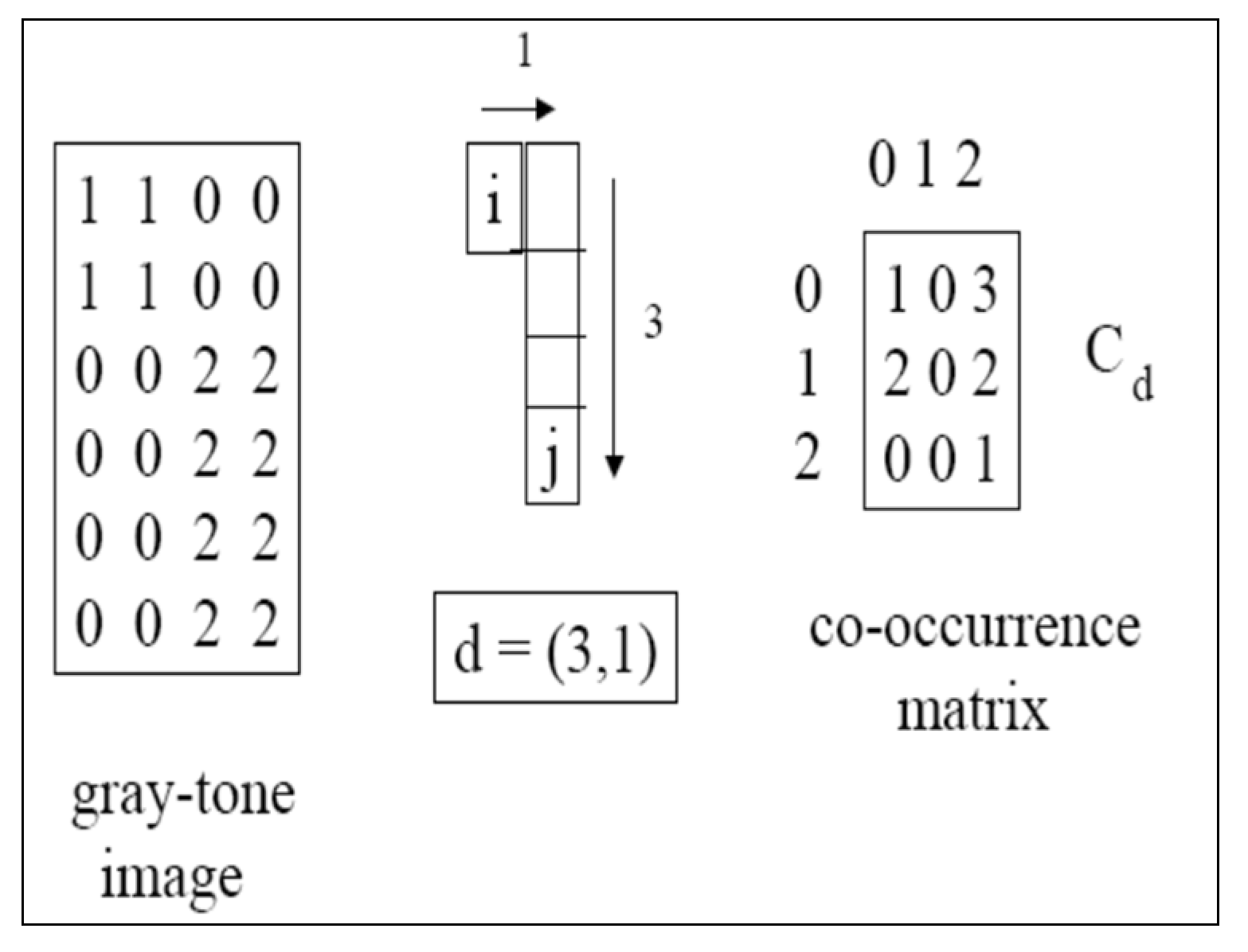
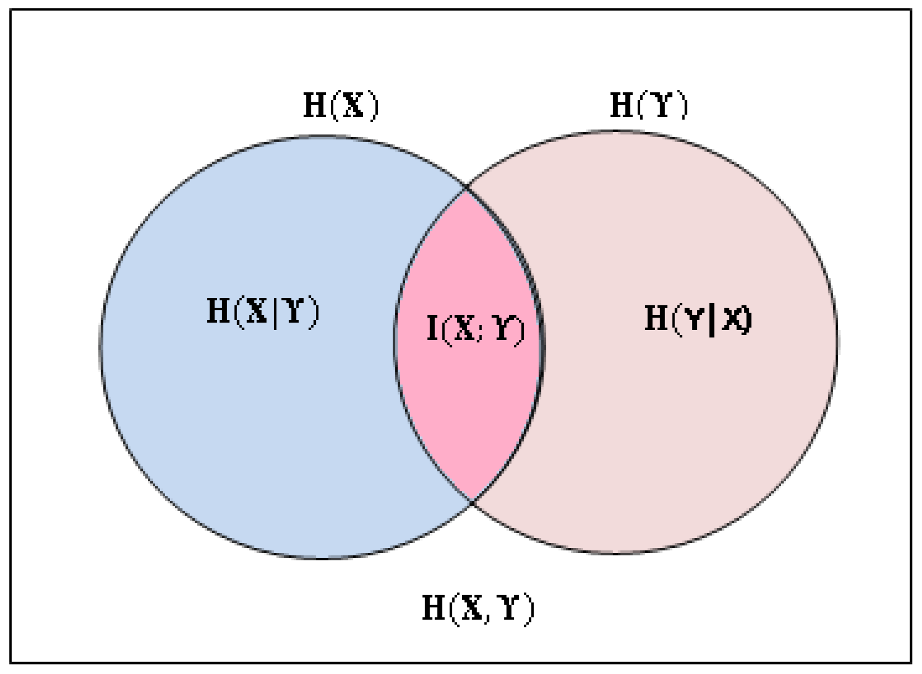

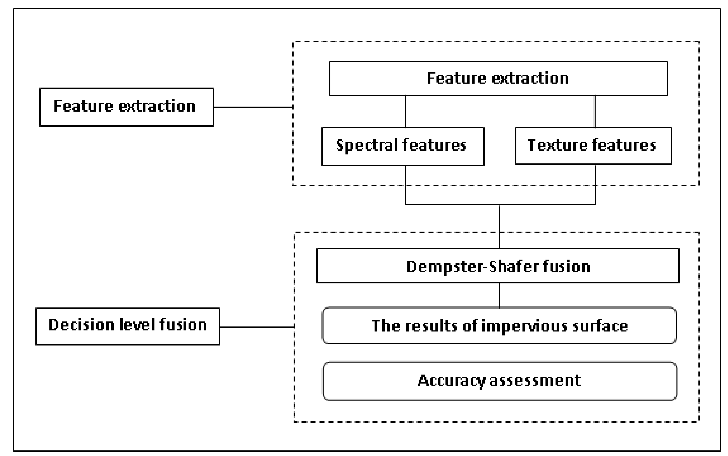

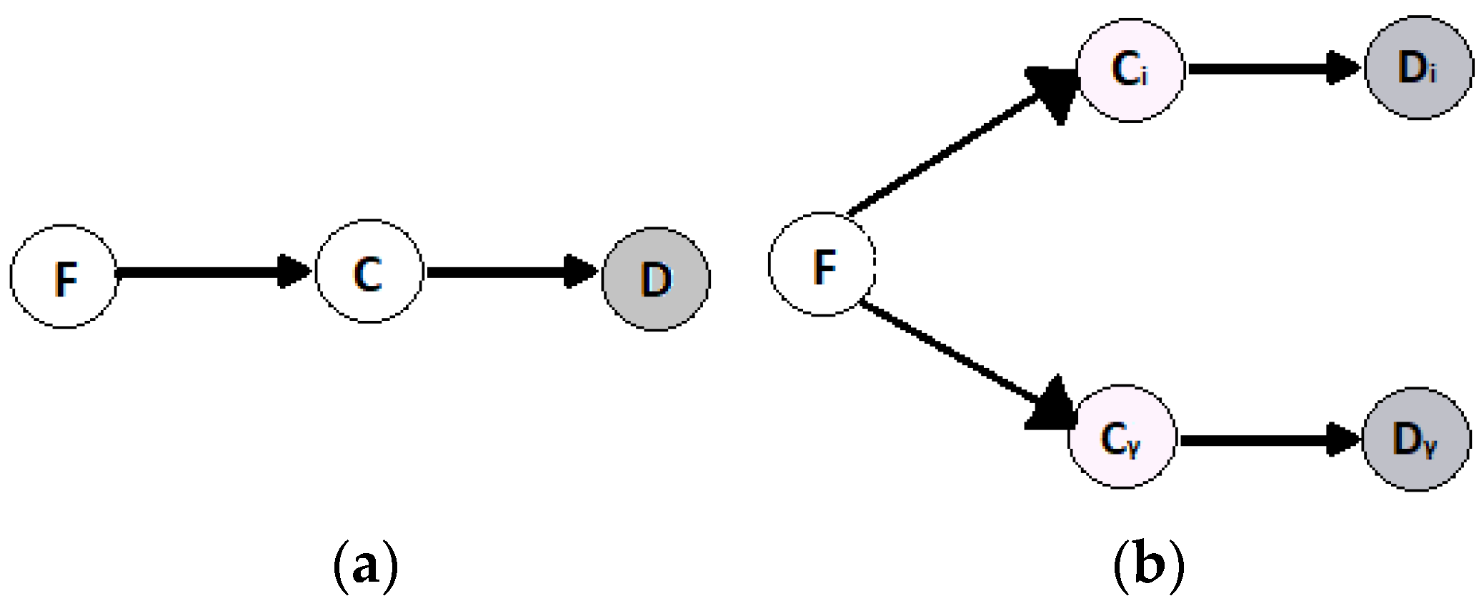
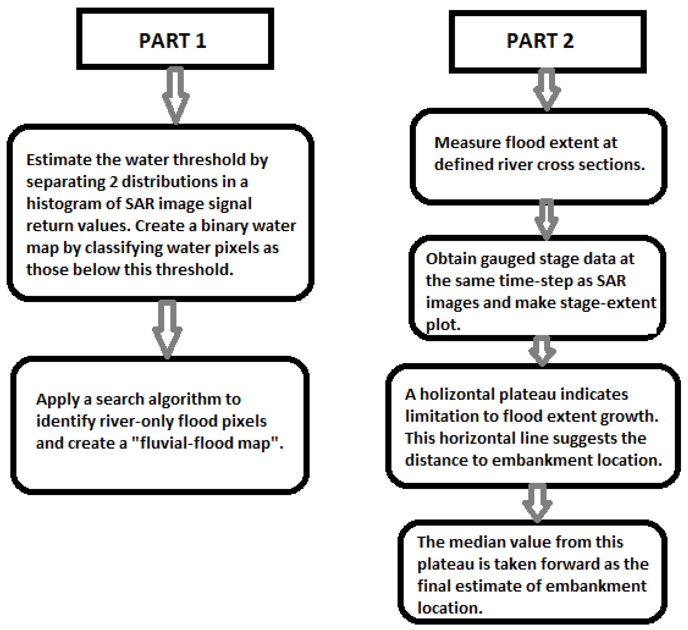
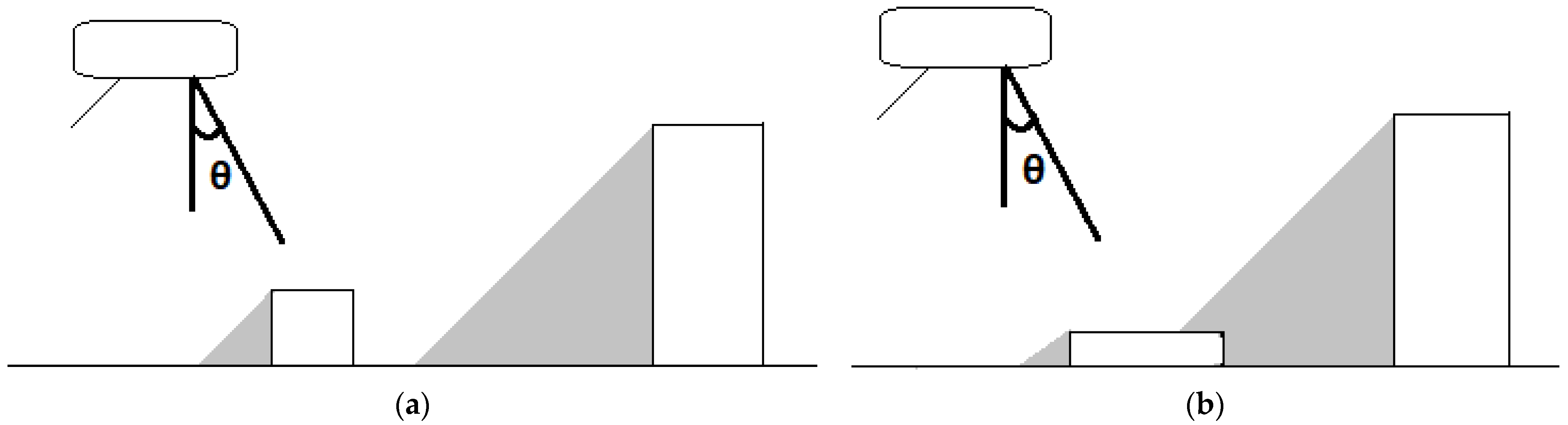

Disclaimer/Publisher’s Note: The statements, opinions and data contained in all publications are solely those of the individual author(s) and contributor(s) and not of MDPI and/or the editor(s). MDPI and/or the editor(s) disclaim responsibility for any injury to people or property resulting from any ideas, methods, instructions or products referred to in the content. |
© 2024 by the author. Licensee MDPI, Basel, Switzerland. This article is an open access article distributed under the terms and conditions of the Creative Commons Attribution (CC BY) license (https://creativecommons.org/licenses/by/4.0/).