Abstract
In recent years, a growing number of sensors that provide imagery with constantly increasing spatial resolution are being placed on the orbit. Contemporary Very-High-Resolution Satellites (VHRS) are capable of recording images with a spatial resolution of less than 0.30 m. However, until now, these scenes were acquired in a static way. The new technique of the dynamic acquisition of video satellite imagery has been available only for a few years. It has multiple applications related to remote sensing. However, in spite of the offered possibility to detect dynamic targets, its main limitation is the degradation of the spatial resolution of the image that results from imaging in video mode, along with a significant influence of lossy compression. This article presents a methodology that employs Generative Adversarial Networks (GAN). For this purpose, a modified ESRGAN architecture is used for the spatial resolution enhancement of video satellite images. In this solution, the GAN network generator was extended by the Uformer model, which is responsible for a significant improvement in the quality of the estimated SR images. This enhances the possibilities to recognize and detect objects significantly. The discussed solution was tested on the Jilin-1 dataset and it presents the best results for both the global and local assessment of the image (the mean values of the SSIM and PSNR parameters for the test data were, respectively, 0.98 and 38.32 dB). Additionally, the proposed solution, in spite of the fact that it employs artificial neural networks, does not require a high computational capacity, which means it can be implemented in workstations that are not equipped with graphic processors.
1. Introduction
In recent years, we have been witnessing a rapid development in Very-High-Resolution Satellite imaging (VHRS). It may be applied in numerous fields: landcover mapping [1,2], urban mapping [3], the detection and tracking of objects [4,5,6,7], maritime monitoring [8,9], automatic building classification, etc., [10,11].
Contemporary very-high-resolution satellites are capable of recording images with a spatial resolution of less than 0.30 m. However, until now, these scenes were acquired in a static way. The new technique of the dynamic acquisition of video satellite imagery has been available only for a few years. It has multiple applications related to remote sensing. However, in spite of the offered possibility to detect dynamic targets, its main limitation is the degradation of the spatial resolution of the image that results from imaging in video mode, along with a significant influence of lossy compression. Satellite observations in video mode offers new possibilities in comparison to traditional satellite systems for the observation of the Earth. This technology may be used to track targets or to capture a sequence of video images instead of a static scene [12,13]. As it has been mentioned before, video imaging is characterized by high temporal resolution; however, at the cost of lower spatial resolution in comparison to VHRS systems. Methods that allow for the improvement of spatial resolution may be divided into two groups: the first one includes multiple-image super-resolution methods [14], while the other one is based on single-image super-resolution [15]. As far as video imaging is concerned, the multiple-image methods cannot always be applied as the content of the image changes too quickly to be able to use a combination of several sequences of images to improve the resolution. Another common barrier is the presence of clouds, shadows, and moving objects, as well as changes in plant vegetation.
However, classical methods of spatial resolution enhancement for image sequences, as well as images acquired from space, often exhibit:
- A lack of improvement in interpretational capabilities.
- The occurrence of spectral distortions.
- Color distortions.
- For pansharpening-based methods, it is necessary to have an identical high-resolution panchromatic image.
- The occurrence of artifacts in the case of video data where objects move quickly and the temporal resolution of the data is low.
- Correctness of operation only for specific types of data.
As a result, one of the solutions to the above problem is the application of Single-image super-resolution (SISR) algorithms that are based on Deep convolutional neural networks (CNNs). In the last decade, many Super-Resolution (SR) techniques were introduced that were developed with the use of deep learning methods. Some of the popular techniques include Generative Adversarial Networks (GAN) [16] and very deep convolutional networks (VDSR) that show promising results on generating realistic HR imagery from low-resolution (LR) input data [17]. Moreover, they show promising potential in terms of their high resolution (HR) and computational speed.
The applications of super-resolution algorithms may be found in multiple research studies. The authors of [18] applied SRCNN and VDSR solutions for Pleiades and SPOT imagery. On the other hand, Lanaras et al. [19] increased the resolution of channels in the Sentinel 2 imagery from 20 m and 60 m to 10 m with the use of high-resolution bands in order to transfer spatial details from lower-resolution channels. The developed architecture was named DSen2 and was based on the EDSR solution [20]. A similar solution was applied in the studies conducted by [21] with the difference that Sentinel-2 images were used to train the neural network in order to improve the spatial resolution for Landsat imagery.
A much greater challenge lies in improving the quality of the image sequences acquired by nanosatellites. In this regard, researchers must consider the following challenges:
- A large number of images (frames), which increases the computational demands on processing units or prolongs the time required for data processing.
- Maintaining the estimation style of images for all images belonging to the sequence.
- The occurrence of noise and disturbances resulting from imperfect optical systems.
- Low temporal resolution due to limited computational power of the computers on board nanosatellites.
The authors of the present article propose a new solution that allows for the improvement of the spatial resolution of video data. This method belongs to the group of Single-Image Super-Resolution (SISR) solutions and it uses the GAN network extended by an encoder–decoder network that is responsible for improving the quality of SR images. The method presented here introduces the following improvements:
- An individual approach to each video frame enables the processing of video data of any temporal resolution;
- The frames are divided into smaller fragments (tiles), which allows the improvement of the spatial resolution of video data of unlimited dimensions;
- The use of a 10% overlap between tiles enables the achievement of the maximum quality of SR images while, at the same time, minimizing the amount of time required to improve the resolution of the video data (a higher overlap leads to a larger number of images to be processed);
- It is recommended to train the network using databases that consist of images of various spatial resolutions, as this allows for the model training to be made even more resistant to the vanishing gradients phenomenon (the probability of its occurrence for satellite data is much higher than in the case of images obtained from the surface of the Earth);
- Developing the GAN network model by layers of the Uformer model (the encoder–decoder network) allows for a significant improvement of the quality of the estimated SR images;
- The application of time windows to connect the tiles estimated by the GAN network generator enables the combination of them into one video data frame;
- The global quality assessment does not reflect the actual quality of the estimated SR images, but the application of the local assessment and image evaluation in the frequency domain enables a better assessment of SR images.
This paper consists of the following sections: Section 2 presents a review of the methods to improve the spatial resolution of video sequences with the use of deep neural networks. The description of the proposed methodology is provided in Section 3. Section 4 contains a description of the research and the results. Section 5 is the discussion, while the final conclusions are presented in Section 6.
2. Related Works
The need to improve the spatial resolution of a sequence of images poses additional requirements: the method’s operation has to be fast (due to a large number of frames), enable processing images of various dimensions, and the estimated frames must be recreated in the same style (as estimation errors will be visible in subsequent images in the sequence). Algorithms based on SISR may be divided into solutions that employ interpolation, reconstruction, and machine learning. The issue of super-resolution is a typical problem of connecting the relations between low-resolution (LR) and high-resolution (HR) images [22]. On the other hand, other sharpening methods, in particular concerning video sequences, were based on motion blurring and hybrid regularization [23]. Yet another method used discrete and stationary wavelet transforms to increase the spatial resolution and to bring out the details of a video sequence [24]. With the development of modern deep learning algorithms, more and more attention has been paid to developing new methods related to the improvement of the spatial resolution of the imagery. One of the first research works was the study by [25], which presented the results of enhancing the resolution of an image with the use of Deep Convolutional Networks. Other authors proposed using an hourglass-shaped convolutional neural network structure (FSRCNN) to accelerate SRCNN [26]. Yet another method that employs the Deep Back-Projection Network (DBPN) allowed for an even eight-fold increase in the resolution of images by connecting a series of iterative up- and down-sampling steps [27]. Furthermore, Yu Xiao et al. [28] addressed the issue of enhancing the spatial and temporal resolution of satellite recordings. They introduced a module of attribute interpolation that is equipped, among others, with multi-scale deformable convolution to predict unknown frames and a multi-scale spatial–temporal transformer is proposed to aggregate the contextual information in long-time series video frames effectively. Other authors [29] introduced the HiRN model that employs the hierarchical recurrent propagation and residual block-based backbone with a temporal wavelet attention (TWA) module. Another solution consists of the application of a generative adversarial network to perform multi-frame super-resolution (MFSR). An example is the MRSISR model [30], which introduces comments to the module generator and space-based net that is responsible for improved information extraction. Jin et al. [31] noted that most of the existing VSR methods focused mainly on the local information between frames, which lack the ability to model long-distance correspondence. In order to solve this problem, they proposed a two-branch alignment network with an efficient fusion module. This solution uses deformable convolution (DCN) and transformer-like attention. Another solution that uses information between frames is the framework model proposed by Liu et al. [32]. These authors proposed a framework based on locally spatiotemporal neighbors and nonlocal similarity modeling. This allowed them to use local motion information without explicit motion estimations. Yet another VSR solution that employs artificial neural networks is the model proposed by He et al. [33]. They proposed a method that consists of three modules: the degradation estimation module (which estimates the blurring and the level of noise in LR images), the intermediate image generation module (that generates frames of intermediate super-resolution), and the multi-frame feature fusion module (feature fusion subnetwork is leveraged to fuse the features from multiple video frames).
Another literature review is [34]. The authors of this publication highlighted the difficulties and challenges of enhancing the resolution of the sequences of images acquired by satellites. They pointed to poor data continuity, global motion due to platform movement, large changes in illumination, large redundancy between video frames, an extreme foreground–background imbalance, a complex background environment, a huge scene size, and, finally, large differences in object scales. Apart from a detailed overview of the methods to improve the resolution of image sequences, the study also contains a wide presentation of Satellite VSR methods. The authors also described the public Dataset: VISO dataset [35], SatSOT dataset [36], and Air-MOT dataset [37]. Another database that has been published in recent years is the Jilin-189 proposed by Wuhan University [38]. Li et al. noted that in the last few years, there has been a dynamic increase in the number of publications concerning VSR.
A review of these publications reveals that multiple methods use SISR solutions to improve the spatial resolution of image sequences. The number of frameworks that present proposals of solutions to the SISR problem is several times higher that the number of solutions that focus on VSR. In the last few years, numerous overviews of the SISR methods were published. An example may be the study by Wang et al. [39]. In 2022, we also noted the problem of enhancing the resolution of imagery acquired by Small Satellites. The publication [40] contains a review of the methods to enhance the spatial resolution of satellite imagery, with particular focus on enhancing the resolution of images acquired by nanosatellites. In our review, we highlighted the methods that employ pansharpening and SISR methods that use interpolation, Digital Image Processing, and artificial neural networks. During our research, we noted that, in spite of their advanced, sophisticated structure, some types of architecture based on convolutional networks cannot be successfully applied in SISR satellite imaging because they do not improve interpretation abilities in spite of the enhanced resolution.
After a series of tests, we found that SR images estimated by SISR algorithms that employ artificial intelligence often had characteristic textures or blurred edges. An example of an algorithm that focuses on removing the noise from an image is the solution proposed by [41]. The authors of [42] modified the variance model based on the edge adaptive-guiding function. It uses an adaptive function that is responsible for enhancing the edges. It employs a standard gradient into the non-linear diffusion term. Another solution [43] is the non-linear filter, whose task is to remove constant-impulse noise (e.g., salt and pepper) from multiple-channel images. The authors of this method performed a fusion of a standard median filter and morphological operation. Among noise removal methods, one may distinguish solutions that employ non-blind techniques [44]. These authors proposed new images prior based on a parameterized scaled Gaussian model and a gamma distribution, with hyperparameters based on the statistical properties of tens of thousands of images. Another solution is the Uformer [45], where the novel, locally enhanced window was introduced (LeWin), with a transformer block and a learnable multi-scale restoration modulator in the form of a multi-scale spatial bias to adjust features in multiple layers of the Uformer decoder. This method stands out for its ability to capture both local and global features of images, making it applicable in noise removal and image deblurring tasks. The resulting images are characterized by a high quality (PSNR/SSIM: 30.90 dB/0.953 for HIDE database [46], 36.19 dB/0.956 for RealBlur-R database [47], and 29.09 dB/0.886 for RealBlur-J database [47]), ref. [45], compared to other methods used for image denoising (for example: Nah [48], DeblurGAN [49,50], DeblurGAN-v2 [51], DBGAN [52], SPAIR [53,54], SRN [55], DMPHN [56], and MPRNet [57]).
3. Methodology
When we were conducting our research on MCWESRGAN (Multicolumn Wasserstein Enhanced Super-Resolution Generative Adversarial Networks) [58], we noted that SR images were characterized by a specific texture. Based on this finding, we decided to search for a method that would improve the quality of images by limiting the occurrence of deformations.
The problem of the quality of interpretation of image context is very important in the case of video data, which contain large, complex patterns that change their position in consecutive images of the sequence. The change in the position of objects in consecutive images in a sequence results from the movement of objects in the image and the movement of the satellite that acquires data. Furthermore, the quality of representation of building infrastructure (including critical infrastructure) and road infrastructure is essential in tasks that consist in detecting smaller objects, e.g., vehicles or airplanes.
During our research, we noted that both classical methods of processing digital imagery and methods of blur removal, i.e., the Lucy–Richardson Algorithm [59] and Wiener deconvolution [60], fail to solve the problem (which was presented in Section 4). Due to that, we decided to find a solution that would employ deep neural networks. Based on empirical experiments, we noted that combining the Uformer model with a MCWESRGAN network allows for the removal of mistakes generated by the SISR network. Thanks to the application of the locally enhanced window (LeWin) Transformer block mechanisms, the extended model interprets the global and local context of an image better. Consequently, the resulting SR images are characterized by higher quality and improved interpretation capacity. Moreover, the conducted literature review demonstrated that expanding SISR algorithms by adding models that improve the quality of estimated SR images was not used by other researchers. Due to that, the proposed solution is innovative and may be commonly applied to enhance the spatial resolution of digital imagery.
This paper presents a method to enhance the resolution of video sequences with the use of Generative adversarial network (GAN) of a small input size (96 × 96 pixels). The effectiveness of the proposed method of image processing was verified with the use of evaluation metrics presented in Section 3.2.
3.1. Proposed Methodology
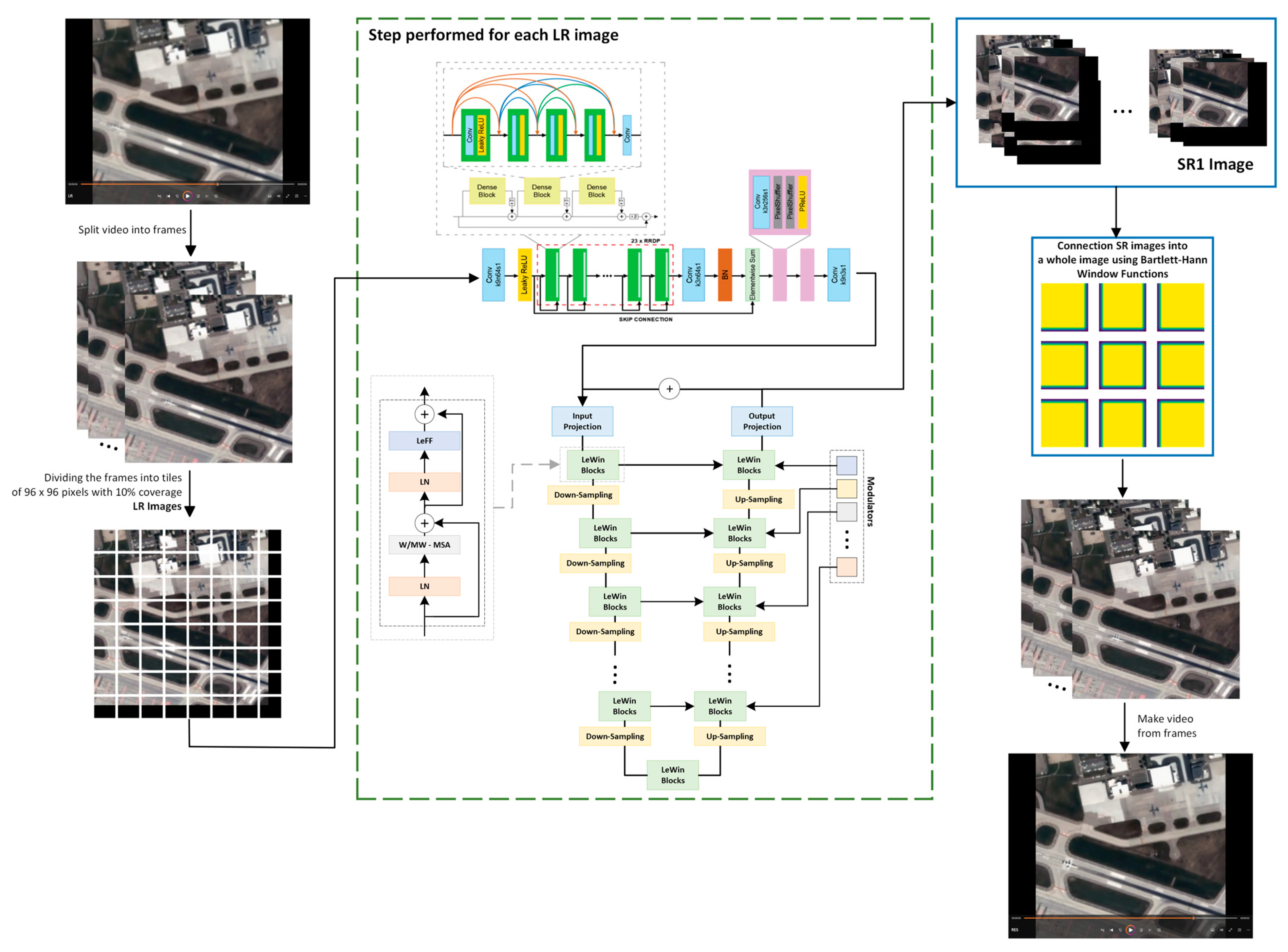
The aim of the conducted research was to develop a method to enhance the resolution of sequences of satellite images while at the same time recreating as much of the informational content of images as possible. For the purposes of our research, we propose an approach that takes into account the Generative Adversarial Networks’ architecture. These networks enable us to generate images of increased resolution by forcing the artificially generated images to be non-distinguishable from original high-resolution images in terms of statistical parameters [16]. The proposed methodology enables the improvement of the spatial resolution of video data that may consist of any number of frames whose size is not precisely defined. It consists of five main stages: (1) loading a single video frame, (2) dividing the frame into smaller tiles (the dimensions are determined by the input_size parameter of the GAN network) with an overlap of 10% (the value of overlap between images was calculated in another research project of the authors [61]), (3) improving spatial resolution with the use of the SISR algorithm (e.g., a GAN network generator), (4) enhancing the interpretational quality of SR1 image with the use of artificial neural networks (Uformer model), and (5) recombining the estimated images (SR2) into a single frame. The diagram of the presented methodology is shown in Figure 1.
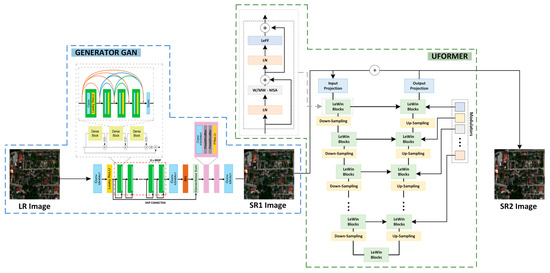
Figure 1.
Diagram of enhancement of spatial resolution of a single video frame.
In order to conduct the tests to determine the quality of the proposed method, the network used as the one responsible for enhancing spatial resolution was the MCWESRGAN network created by the authors, which was described in detail in the publication [58]. The quality of SR images was improved with the use of the Uformer algorithm that employs the locally enhanced window Transformer block. The resulting images were combined into a single frame with the use of the Bartlett–Hann Window Functions.
3.1.1. MCWESRGAN
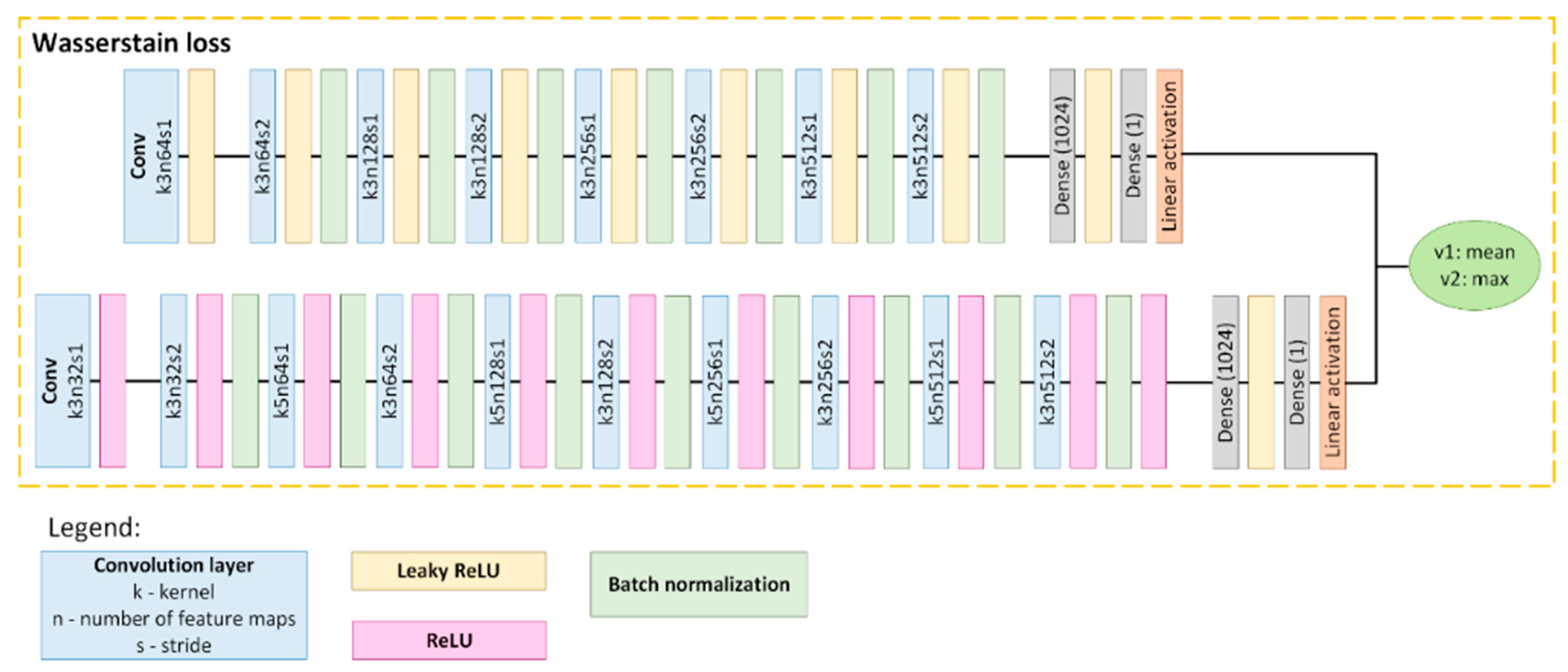
The resolution of each tile was enhanced with the use of the MCWESRGAN model designed by the authors. When preparing the MCWESRGAN network, we modified one of the most popular SISR networks, i.e., the ESRGAN [62]. In our work, we focused mainly on the discriminator and the generator learning technique. The discriminator of generative adversarial networks (GAN) is a convolutional neural network that is responsible for the evaluation of images during the training of the generator. In the MCWESRGAN network, we used a discriminator consisting of two branches: the first of these classifiers has the same structure of layers as the discriminator of the SRGAN network, the second one was expanded by adding another convolutional layer and, for every layer, ReLU activation was applied. Moreover, for even convolutional layers, the kernel size was increased to 5 (pixels) (Figure 2). The introduced modification allowed for a much better assessment of the generator work quality (two scores are received from each critic), which, in consequence, will enable the acceleration of the generator training process.
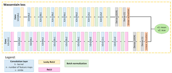
Figure 2.
Discriminator model [58].
The MCWESRGAN network generator was trained with the use of Wasserstein Loss. The main task of this method is to minimize the distance between the HR and SR images. The distance is determined with the use of the Wasserstein distance method (Equation (1)).
where , —probabilistic measures, D:, , W is Wasserstein distance, are functions in the set X, and is joint probability distribution.
The aim of training the MCWESRGAN network with the use of Wasserstein Loss is to strive to achieve alignment between the generator. For this purpose, Kantorovich–Rubinstein duality is used (Equation (2)) [63,64].
where is real data distribution, is the distribution of the parametrized density , and .
For GAN (composed of a generator and a discriminator), Wasserstein Loss takes Equation (3).
where is data distribution, is the model distribution implicitly defined by = G(z), z ∼ p(z), and is set of 1-Lipschitz functions.
The introduced modifications allowed us to significantly (even by 10 times) shorten the time required to train the generator while improving the quality of super-resolution (SR) images, which has been proven in our paper.
3.1.2. Uformer
Training a GAN network is a very demanding process, during which one may often encounter the phenomenon of exploding or vanishing gradients. We discussed this phenomenon in detail in one of our other works [61]. This phenomenon may be reduced by decreasing the learning parameter, which allows to limit the problem of vanishing gradients and, in consequence, to achieve the optimum alignment of the model. However, this solution has one disadvantage, which is the emergence of a specific, unnatural texture in SR images (visually, it resembles a combination of deblurring, denoising, and deraining). In order to avoid this phenomenon, the MCWESRGAN network generator was expanded by adding the Uformer model presented by Zhendong Wang et al. [45]. The authors of this model introduced the locally enhanced window (LeWin) transformer block and a learnable modulator. Moreover, the authors recommended using Charbonnier loss [65,66] to train this model.
The Uformer model is of the nature of a classical U-shaped encoder–decoder network (a diagram of the network is presented in Figure 1). Additionally, skip connections were used between the encoder and decoder, which enable adding the features detected by the algorithm to the input image (). The first stage of operation of the model is to extract low-level features with a convolutional layer from a kernel of the size 3 × 3 and activation LeakyReLU. Then, the tensor undergoes further encoder stages, where each of the stages contains a stack of the LeWin Transformer blocks and one convolutional down-sampling layer (stride: 2). Additionally, LeWin uses the self-attention mechanism for capturing long-range dependencies. Moreover, thanks to the overlapping of windows on feature maps, it derives the calculation cost that results from the use of self-attention. Apart from that, the authors of this solution provide an example, where for feature maps, and the l-th degree of the encoder, feature maps equal . The encoder of the model ends with a bottleneck created from the stack of LeWin Transformer blocks.
The task of the module is to obtain information about the local context of “contaminated” pixels in order to restore their “clean” version. For this purpose, LeWin transformer blocks are used. Moreover, the authors of this solution introduced a convolution operator into the Transformer to capture useful local context. In the feature maps, the LeWin Transformer block meets the normalization layer (LN) first. Then, it is transferred to the Window-based Multi-head Self-Attention (W-MSA) that uses self-attention inside the non-overlapping local windows. In the next step, the skip connection is used to add this result to input feature maps and the result is transferred to the next normalization layer. The normalized tensor is transmitted to the locally enhanced Feed-Forward Network (LeFF), and the resultant tensor is once again (with the use of skip connection) added to the feature maps that were transferred to the LeWin Transformer blocks. Furthermore, the application of the bottleneck stage with a stack of LeWin Transformer blocks allows the capture of additional dependencies of features, and if the size of the window equals the size of the Transformer block, global dependencies are captured.
The network decoder is equipped with modulators. The aim of this module is to calibrate the features, which enable recovering a larger number of details (by taking into account the characteristics of interfering patterns). The multi-scale restoration modulator is embedded in each block of the LeWin Transformer, taking a form of a tensor of the shape W × W × C, where W is the window size and C is the size of the channel of the current feature map. The modulator takes the form of a matrix that is added to all nonoverlapping windows before the self-attention module.
The branch of the decoder module is responsible for the reconstruction of features. It is built of the up-sampling layer and a stack of LeWin Transformer blocks. In this model, the convolution layers were replaced with transposed convolution (convolution: 2 × 2, stride: 2). In accordance with the principle of functioning of transposed convolution, it is responsible for increasing the feature maps twofold and reduces half of the feature channels. The authors of the solution used the LeWin Transformer blocks to learn to restore the image. In order to obtain the resulting image , the authors propose 3 × 3 convolution layer, which will allow for the feature maps to be flattened to 2D feature maps. The resultant image is a result of adding features to the input image .
3.1.3. Bartlett–Hann Window Function
The Bartlett–Hann Window Function was used to recombine the SR images into a single frame. This Window Function was not selected at random. The choice was motivated by the research results presented by the authors in the publication [61], which provides a comparative analysis of various Window Functions for various degrees of overlapping between neighboring tiles. During the research, it was noted that the best quality of the resultant image was obtained when the tiles of the SR image were combined with the use of Hann, Hann–Poisson, Bartlett–Hann, or Triangular window functions.
For the purposes of this research project, the Bartlett–Hann Window Function was used to recombine the tiles into a single image. In this method, for each pixel in the image fragment (which is in the area of overlap between images), the weight is calculated (Equation (4)), with which the given pixel will be added to the resultant SR image.
where n is position of the pixel in the image and N is tile size.
3.2. Evaluation Metrics
The quality assessment of the resulting SR images consisted of three stages. The first one consisted of conducting a global quality assessment of all SR images before combining them into images of the sequence. This was performed with the use of the most popular metrics that are used in the fields of remote sensing and computer vision (Table 1).

Table 1.
Presentation of the main evaluation metrics.
When performing the global assessment of the quality of SR images, one should note that the results are the average evaluation of the whole image. Due to that, it is difficult to determine how specific areas of the image are represented in the SR images. As a result, the second stage of the SR image evaluation involves local assessment. In this method, the SR image is divided into smaller fragments of a defined surface area, and then evaluation metrics values are calculated for these fragments. This method enables one to determine which areas of the SR image are better represented, and which are poorer.
The final method of assessing the quality of SR images is the determination of the physical enhancement of the spatial resolution of SR images by means of power spectral density analysis (PSD) of the image. PSD explains the distribution of the frequency of signal power. This method allows you to determine the improvement in the ability to detect objects in the image using the Ground Resolved Distance (GRD) parameter.
4. Experiments and Results
4.1. Datasets
While training generative adversarial networks, one should bear in mind that this type of network is very prone to the phenomenon of vanishing gradients. During the tests, it was found that databases that consisted of images of varied spatial resolution were more stable during the training of the generator. Due to that, the final database that was the basis for training the prepared network contained images obtained by unmanned aerial vehicles (UAV), optic sensors mounted on airplanes, observation satellites, and nanosatellites. As a result, the created database contained images of a spatial resolution ranging from 0.15 m to 20 m and consisted of 100,000 images. Such a diversified database was created as a result of combining the Dataset for Object deTection in Aerial Images (DOTA) [70], fragments of aerial images (that were a result of dividing the orthophotomap), imagery acquired by the WorldView-2 (WV2) satellite, the Jilin-1 database [38], and other data acquired by the SkySat-1 and Jilin-1 nanosatellites. The Jilin database contains video data acquired by the Jilin-1 satellite. It consists of 201 clips, where each clip contains 100 images of the size of 640 × 640 pixels. Apart from that, other video sequences captured by the Jilin-1 mission were added to the database [71]:
- Beirut in Liban—collected on 06 October 2017, the resolution: 1.12 m, the frame size: 1920 × 1080 pixels, 25 frames per second (FPS), and video duration: 32 s.
- Florence in Italy—collected on 10th September 2018, the resolution: 0.9 m, frame size: 3840 × 2160 pixels, 10 FPS, and video duration: 31 s.
- Other materials added to the database were the video sequences collected by SkySat-1 from Las Vegas (25 March 2014), Burj Khalifa (9 April 2014), and Burj al-Arab (1 February 2019) [72].
In order to train the models that are responsible for enhancing the resolution, it is necessary to prepare high-resolution (HR) and low-resolution (LR) data. To create the database used here, most of the HR images were prepared by dividing images into tiles of the dimensions of 384 × 384 pixels, and the corresponding LR images were prepared as a result of sampling the HR images to the dimensions of 96 × 96 pixels. The exceptions were the satellite scenes acquired by the WV2 satellite. In this case, the LR database was created by dividing the multispectral imagery. To prepare the HR database, we used an image whose resolution was improved using pansharpening (the Gram–Schmidt method).
4.2. Methodology of Processing Video Data
The process of enhancing the spatial resolution of a sequence of images may be divided into three main stages: (1) preparing data, (2) enhancing spatial resolution, and (3) combining the images into sequences. The detailed flowchart is presented in Figure 3.

Figure 3.
The flowchart of the algorithm.
The process of preparing data for spatial resolution enhancement starts with loading a video file, which, in the next step is divided into single frames. Then each of the frames is divided into smaller tiles (LR images). Due to the fact that the MCWESRGAN network was used to improve the resolution, the frames were divided into fragments of the dimensions of 96 × 96 pixels (the size was determined by the input size parameter of the GAN network used). If the size of the tile is smaller than the input size parameter, the missing areas are filled with pixels of the digital number (DN) equal to 0 (black stripes that are shown in Figure 3). Data prepared in this wat are then transferred to the MCWESRGAN network with the added Uformer network. This module first enhances the spatial resolution of the resulting LR image, and then improves its quality with the use of the Uformer model. When the spatial resolution of all tiles belonging to a single frame has been improved, the third stage of the proposed methodology commences. In this module, the tiles are combined into a single frame with the use of the Bartlett–Hann Window Function, and when all frames have been processed, they are recombined into a sequence of images.
4.3. Implementation
The SISR model was trained on a Nvidia TITAN RTX 24 GB graphics card, Intel Xeon Silver 4216 processor, and the Ubuntu 18.04 operating system. The network training parameters are presented in Table 2.
Table 2.
Network training parameters.
The training dataset was used to train the model that is responsible for enhancing the spatial resolution of LR images. This was the basis for estimating the weights between the layers of the model. The weights were updated based on the results of the assessment of the network model with the use of validation data. Adam optimization was used to find the target function. The application of this model enables the high-quality achievement of the model in a short time. Moreover, as a result of training the generator of the GAN network that is responsible for the SISR of data acquired from space altitude, it is more resistant to the vanishing gradient phenomenon (in comparison to other optimization methods, e.g., SGD, RMSprop, and Adagrad).
4.4. Results
The proposed MCWESRGAN model, expanded by adding the Uformer model layers, was tested on a set of video frames from the Jinlin-1 dataset (the test dataset). To assess the results, the metrics presented in Table 1 were employed. The obtained results were compared to the SR images estimated by the MCWESRGAN model, from which the specific texture was removed with the use of the Lucy–Richardson Algorithm and Wiener deconvolution. The Lucy–Richardson Algorithm is an iterative method that enables the removal of blurring and noise from an image. The functioning of the algorithm may be presented in the form of Equations (5) and (6).
where is the image estimated in iterations, is the pixel value, and is the spatial displacement between the value of the source pixel and the value of the observation pixel .
On the other hand, Wiener deconvolution enables the determination of the range of frequency of the non-disturbed signal. Thanks to this property, it is possible to remove blurring from the image. If the blurring is large, a disadvantage of the solution is the fact that the characteristic texture emerges in the image. In the frequency domain, the Weiner Filter was presented in Equation (7).
where G(t), H(t) are the Fourier transforms g(t) and h(t), S(t) is the average spectral density of the power of the original signal x(t), N(t) is the average spectra density of the noise power, and * is the feedback operation.
In order to remove blurring, it is necessary to possess information about the characteristics of the image deformations and the balance parameter. The aim of this parameter is to reduce the occurrence of noise artifacts in the resulting image, i.e., to maintain the balance between the reconstructed image and the image containing noise.
The evaluation of the estimated high-resolution images started with the assessment of the results, and the values of the described quality evaluation indicators for the whole test dataset were calculated.
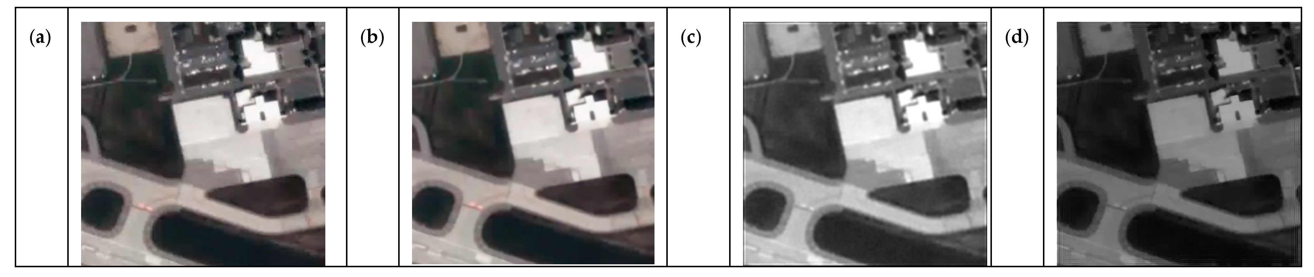
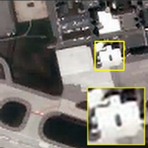
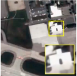
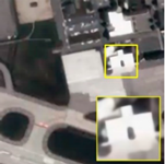
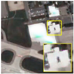
In Table 3, we presented a qualitative analysis of the test dataset, where we compared the SR images generated by the MCWESRGAN generator enhanced with (1) the Lucy–Richardson Algorithm, (2) Wiener deconvolution, and (3) the Uformer network. Additionally, in Figure 4, we provided examples of images. The results unequivocally demonstrate the superiority of the MCWESRGAN network extended with the Uformer network over the generator enhanced with the Lucy–Richardson Algorithm and Wiener deconvolution. In the case of SR data generated using the Lucy–Richardson Algorithm, in addition to the deterioration in quality, artifacts are visible (mainly at the edges of the image) along with significant color changes. Conversely, for SR images generated using Wiener deconvolution, the distortion of colors is much greater (confirmed by the qualitative analysis).
Table 3.
Quality analysis of the test database. The best results are marked in green and the poorest ones in red.

Figure 4.
Examples of images from test data with quality results are shown in Table 3: (a) HR image, (b) MCWESRGAN with Uformer, (c) MCWESRGAN with Lucy–Richardson Algorithm, and (d) MCWESRGAN with Wiener deconvolution.
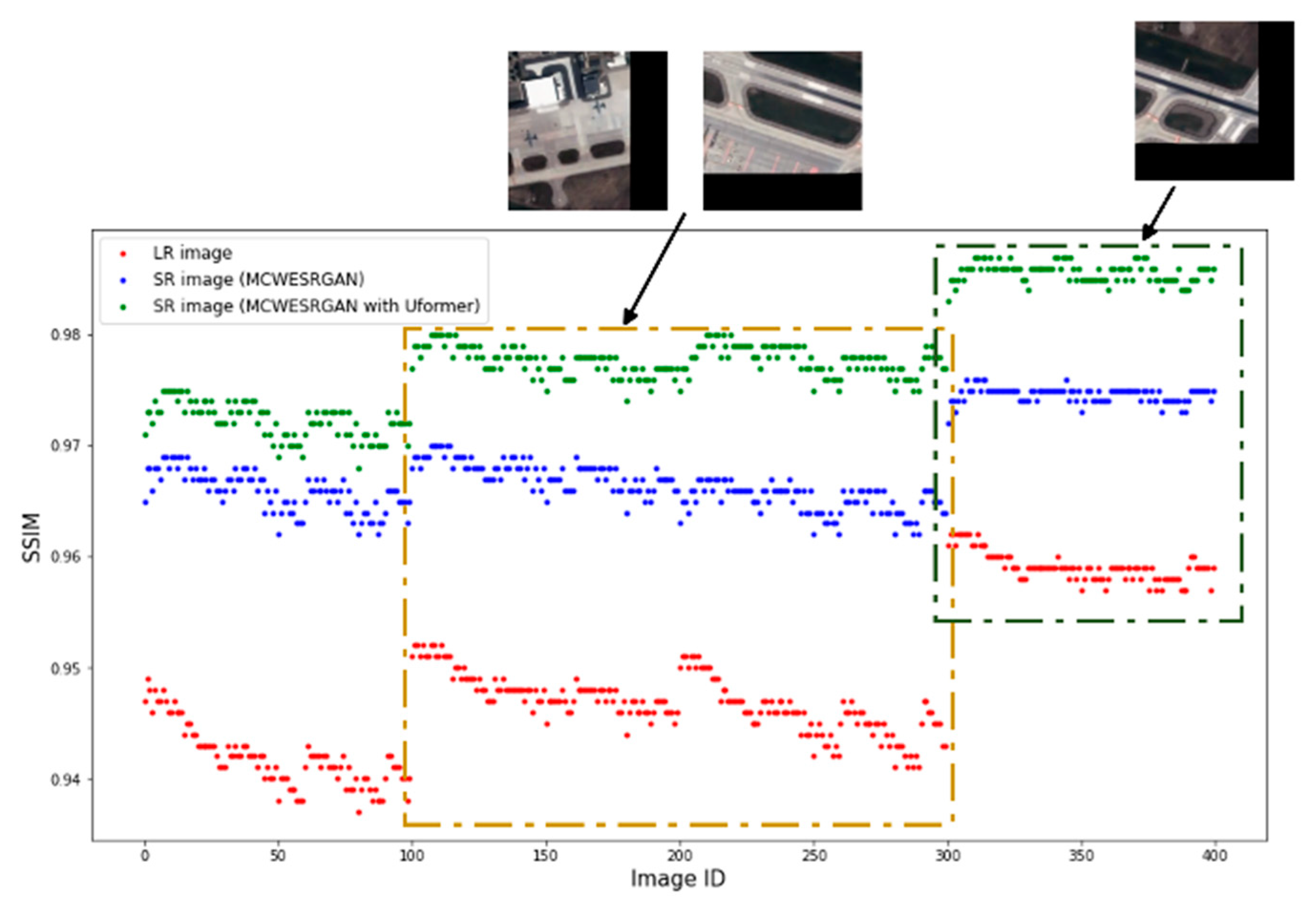
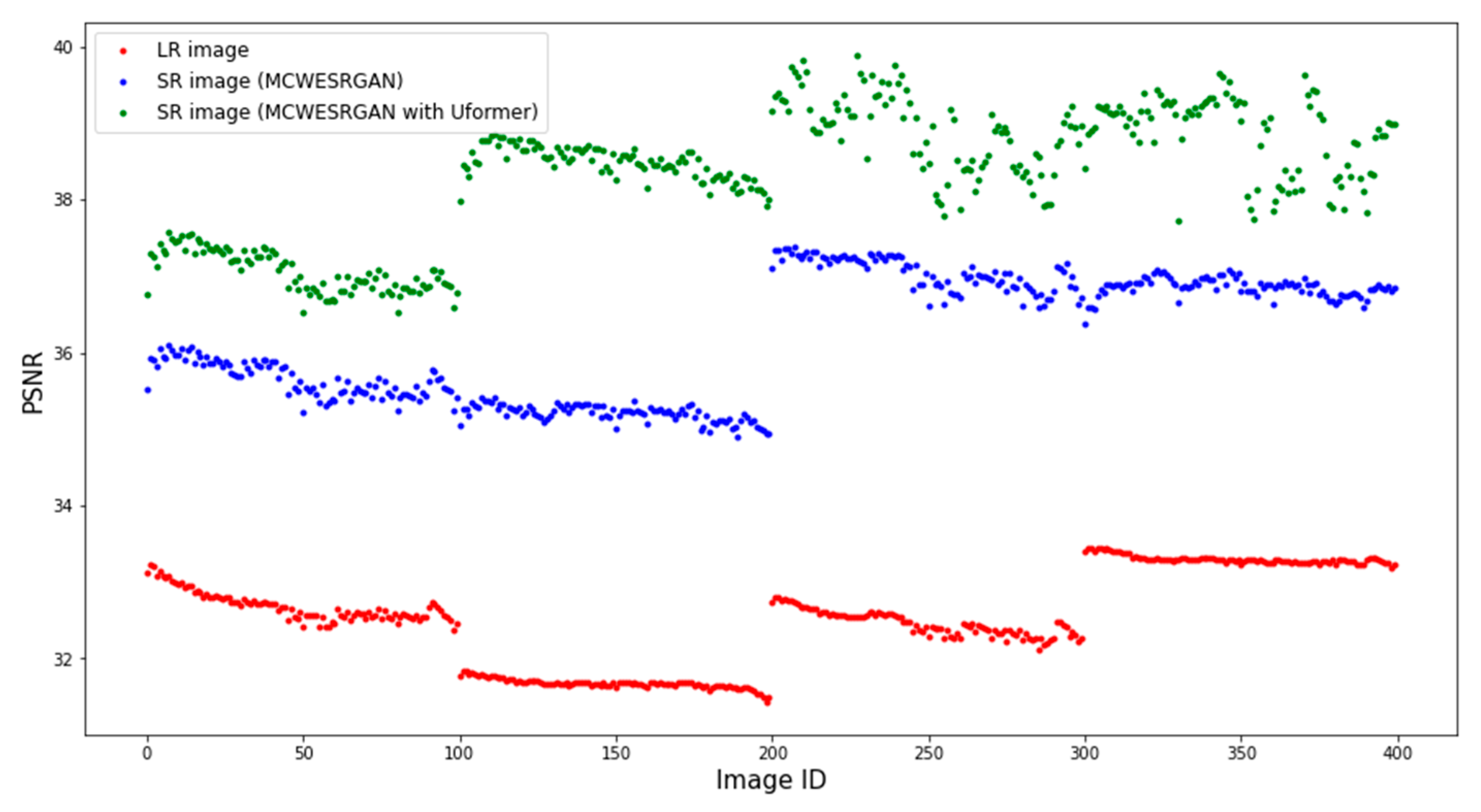
Additionally, Figure 5 and Figure 6 show the differences in the values of the SSIM and PSNR metrics for a random video, where, however, the frame has the dimensions of 160 × 160 pixels (the Jinlin-1 database). Due to the size of the frame, it was divided into four tiles (pixels of DN = 0 were added in the second column and the second line of tiles so that the dimensions would equal the input size). The ID of the image is marked on the X axis of the diagrams. Analyzing the obtained results, one may notice that groups of images of a similar quality exist. Images with ID300-400 are characterized by the highest quality, but they have the added groups of pixels of DN = 0, which increase the metrics of the quality assessment. At the same time, one may notice that the SR images estimated by the MCWESRGAN network with the Uformer model are characterized by higher quality in all fragments of the image.
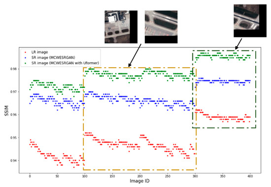
Figure 5.
Structural similarity between the estimated images (tiles) (SR) and the reference HR images.
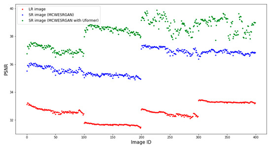
Figure 6.
Peak signal-to-noise ratio (PSNR [dB]) between the estimated images (tiles) (SR) and the reference HR images.
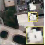
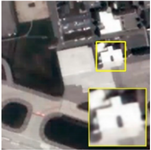
In order to improve the evaluation of the estimated image, local image evaluation was used for the resulting frames (after the tiles had been combined with the Window function). Due to the fact that the size of the assessed resulting frames equalled 640 × 640 pixels, it was assumed that the local assessment would be conducted on image fragments of the size of 20 × 20 pixels. The illustrations below (Figure 7 and Figure 8) show the results of the local assessment conducted with the use of the SSIM and PSNR metrics. In the case of the SSIM metric, the majority of the analyzed areas are marked in yellow, indicating a value of the metric exceeding 0.97. There are only isolated areas with a low estimation quality. However, a local assessment using a PSNR enables a more precise analysis of the image—the differences between the adjacent areas under examination are greater. Based on a local assessment using a PSNR, it can be inferred that moving objects (the airplane on the runway) or small objects of irregular shapes were estimated with high quality, although it was slightly lower than that of parking areas, the runway, and taxiways.
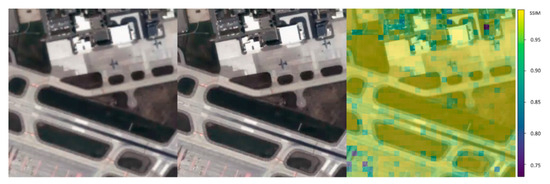
Figure 7.
Local assessment—SSIM metrics (for the evaluated field of the size of 20 × 20 pixels).
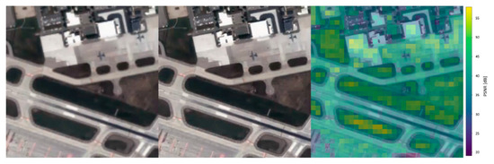
Figure 8.
Local assessment—PSNR metrics (for the evaluated field of the size of 20 × 20 pixels).
Another method to assess the quality of SR images is PSD analysis. The PSD describes the distribution of the frequency of the power signal. This allows for the determination of the smallest size that may be identified in the image.
Figure 9 presents the PSD analysis for the x and y directions. The PSD analysis reveals a high similarity between the signal power frequency distribution in the HR image (yellow curve) and the SR image (green curve), in particular, in the vertical direction of the image (the y direction). In the horizontal direction, resolution enhancement is noticeable for a spatial density of approx. 100 [1/100 m], and in the vertical direction of approx. 120 [1/100 m]. As a result, the value of the GRD parameter on the x direction is GRDx = 2.1 × GSD, and in the y direction, GRDy = 2.5 × GSD. The obtained values confirm that the value of the GRD parameter for high-contrast objects should take the value no lower than two times the GSD.
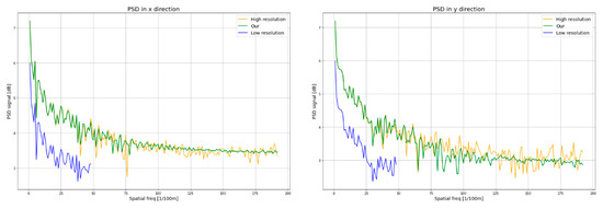
Figure 9.
PSD diagram on the x and y directions for a sample image.
5. Discussion
The proposed methodology of enhancing the resolution of a sequence of images consists of three main stages: the preparation of the images, enhancing the spatial resolution, and combining the estimated images into a sequence. The structure of this solution enables one to use other SISR algorithms that use artificial neural networks. During the research, the authors compared the quality of the enhancement of the spatial resolution of images with the use of various methods using convolutional networks. Additionally, each of the analyzed SISR models was extended by adding the Uformer model, which allowed for a better evaluation of the influence of the Uformer model in the quality of the resultant SR images. The results of the global quality assessment of the test dataset are presented in Table 4. Apart from that, examples of SR images estimated by the analyzed SISR models are provided in Appendix A and Appendix B.
Table 4.
Quality assessmentof convolutional network models dedicated to SISR. The best results are marked in green, the second in yellow, and the worst in red. “*” marks the SISR models with added Uformer network layers.
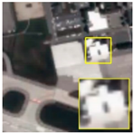
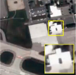
The analysis of the presentation of SR images generated by various SISR solutions that employ convolutional networks (CNN) revealed large differences, in particular in the representation of the edges of anthropogenic objects (i.e., objects created by humans). An example of such an object was marked with a yellow frame (Table 5), and the magnified image is in the bottom-right corner of the illustration. Additional examples are provided in Appendix A and Appendix B. Many of the analyzed models, e.g., EDSR, FSRCNN, SRCNN, SRGAN, and ESRGAN, make errors during the representation of HR images. In images that were estimated with those methods, the edges of objects (even those with high contrast between them and the background) are blurred and their corners are rounded. This visual assessment is confirmed by the qualitative analysis, which was performed with the use of the metrics presented in Section 3.2. The MCWESRGAN architecture designed by the authors and expanded by adding Uformer layers enables the highest quality of enhancing the spatial resolution (SSIM = 0.98, PSNR = 38.32 dB). For the purposes of the conducted research, the authors expanded the most popular models responsible for SISR by adding layers of the Uformer model. The aim of the research was to provide a better assessment of the influence of the Uformer model on the quality of the estimated SR images. In most cases, the obtained results confirmed the beneficial effects of developing the SISR models by adding Uformer network layers. However, for models ESPCN, RDN, and SRDenseNet, a slight deterioration in the quality of SR images was observed (e.g., for the RDN network, the decrease in the PSNR was 0.14 dB).
Table 5.
Examples of SR image fragments estimated by different convolutional network models.
In order to improve the assessment of the SR images that are presented in Table 4, the SR images were transformed with the Fourier domain. Images estimated with MCWESRGAN, for which attempts were made to improve the quality of the estimated image by applying the Lucy–Richardson Algorithm and Wiener deconvolution, were added to the presentation. The aim of including these images was to compare them (where their quality is worse than that of SR images generated by MCWESRGAN) with images estimated with the use of other SISR models.
The transformation of the image with the Fast Fourier Transform (FFT) allows the movement from the spatial domain to the frequency domain while maintaining all attributes of the image. Decomposing an image into sines and cosines of varying amplitudes and phases enables one to distinguish mistakes in the image (Figure 10). Considering the results of the qualitative analyses that are presented in Table 4 and Table 5, one may notice that the poorest quality of the estimated images is obtained if the quality of the SR images obtained with the use of the MCWESRGAN generator is “enhanced” using Wiener deconvolution or the Lucy–Richardson Algorithm. These conclusions are confirmed by the images presented in the frequency domain. These images contain low-frequency areas that are located at a large distance from the point of the coordinates (0,0) (the (0,0) point is situated in the center of the image and it corresponds to the intensity of the constant part of the original function). A similar phenomenon occurs in the SR images that were estimated by the SRGAN, FSRCNN, and EDSR models. An interesting case is the image in the frequency domain that was estimated by ESPCN. During the quality assessment, SR images estimated with the ESPCN model were characterized by high quality, but the analysis of sample SR images in the frequency domain revealed low frequencies that were located approximately 130 pixels from the centre of the image. This phenomenon may result from the fact that areas of the image are represented by pixels of a similar DN value and by the stepped representation of object edges (which is confirmed by the visual assessment of the estimated images).
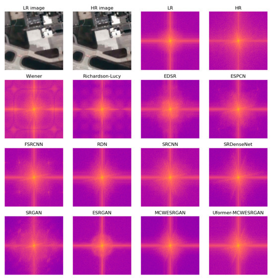
Figure 10.
Images in the frequency domain.
The proposed method consists of several stages that occur consecutively. Thanks to its multiple-stage structure, the proposed solution does not require a large computational capacity. This feature allows the model to be operated on workstations that are not equipped with graphics processors (GPU). The computational capacity of the workstation determines only the duration of processing image sequences. Table 6 presents a comparison of the working times of the module that enhances spatial resolution of video data that consist of 100 frames of the dimensions of 120 × 120 pixels. The presentation demonstrates that the proposed algorithm may be implemented even on hardware that is not equipped with a graphics processor. However, the use of a graphics card significantly shortens the time of processing the sequence of images.
Table 6.
Comparison of the time required to process a single video on various computational units.
The obtained results confirm that it is reasonable to expand the MCWESRGAN model by adding layers of the Uformer network. This modification significantly improves the quality of SR images, and, in consequence, the interpretation capacity. However, the disadvantage of this solution is the prolonged duration of the work of the module that is responsible for enhancing the spatial resolution of the image in the sequence. It takes 0.03 s to enhance the spatial resolution of a single tile with the MCWESRGAN model (without the Uformer layers) (with the use of GPU), which means that the process is over in a time six times shorter than with the use of the MCWESRGAN model expanded by adding Uformer layers.
6. Conclusions
The authors of the present article have proposed a new methodology to enhance the spatial resolution of video data. This solution may, in particular, be applied to sequences of images acquired by nanosatellites. The obtained results demonstrate a fourfold increase in the spatial resolution of low-resolution images, while at the same time, the interpretation capacity has increased by more than two times. Moreover, the development of the generator that is responsible for improving the spatial resolution enabled the improvement of the structural similarity between HR and SR images by approx. 0.02, and the peek signal-to-noise ratio increased by over 2 dB (the average value of the SSIM parameter for the test data increased from 0.96 to 0.98, and the average PSNR value increased from 36.21 to 38.32 dB). The proposed methodology may be applied to issues related to the enhancement of the resolution of images and video sequences obtained by nanosatellites, which require the application of single-image super-resolution (SISR) methods. Apart from that, enhancing the spatial resolution with the use of the methodology described here does not require a large computational capacity (this is required only at the stage of training the model), so it may be used on workstations that are not equipped with graphics processors.
The conducted research focused on proposing a new methodology to enhance the spatial resolution of images obtained from space altitudes. At the same time, it was noted that sequences of images captured by small satellites were characterized not only by a relatively low spatial resolution, but also by a low temporal resolution (approx. 10 frames per sec.) in comparison to aerial systems. This limitation was clearly noticeable during the observations of moving objects (such as an airplane during take-off). Due to that, further works on enhancing the quality of the sequences of images acquired by nanosatellites will focus on improving their temporal resolution.
Author Contributions
Conceptualization, K.K.; methodology, K.K. and D.W.; software, K.K.; validation, K.K.; formal analysis, K.K. and D.W.; investigation, K.K. and D.W.; resources, K.K.; data curation, K.K.; writing—original draft preparation, K.K.; writing—review and editing, D.W.; visualization, K.K.; supervision, D.W.; project administration, D.W.; funding acquisition, D.W. All authors have read and agreed to the published version of the manuscript.
Funding
This research was funded by the Military University of Technology, Faculty of Civil Engineering and Geodesy, grant number: UGB/706/2024/WAT.
Data Availability Statement
Data will be made available on request.
Conflicts of Interest
The authors declare no conflicts of interest.
Appendix A
Table A1.
Models extended with Uformer network layers are marked by adding “*” to the name.
Table A1.
Models extended with Uformer network layers are marked by adding “*” to the name.
| Image 1 | Image 2 | Image 3 | Image 4 | Image 5 | |
| LR | 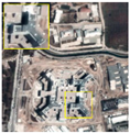 | 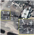 | 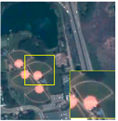 |  | 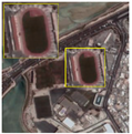 |
| EDSR | 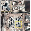 | 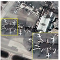 |  | 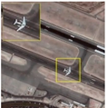 | 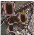 |
| EDSR * | 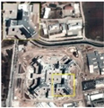 | 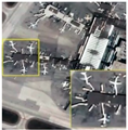 | 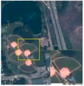 | 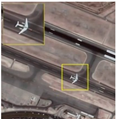 | 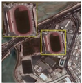 |
| ESPCN | 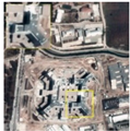 |  | 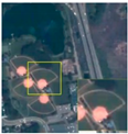 | 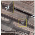 | 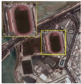 |
| ESPCN * | 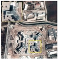 | 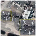 | 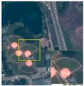 | 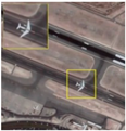 | 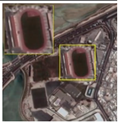 |
| FSRCNN | 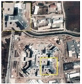 |  |  |  | 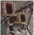 |
| FSRCNN * |  | 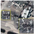 |  |  | 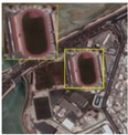 |
| RDN | 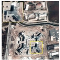 |  | 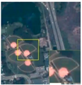 |  | 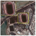 |
| RDN * | 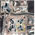 |  | 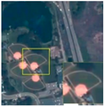 |  | 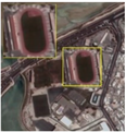 |
| SRCNN | 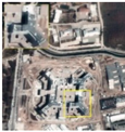 |  | 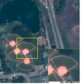 |  | 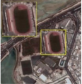 |
| SRCNN * | 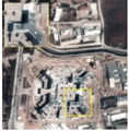 |  | 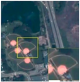 | 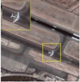 | 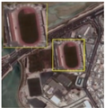 |
| SRDenseNet | 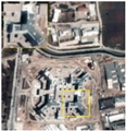 | 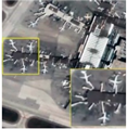 | 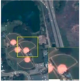 |  | 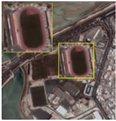 |
| SRDenseNet * | 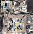 |  |  | 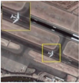 | 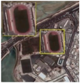 |
| SRGAN | 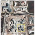 | 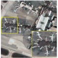 | 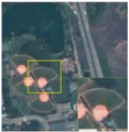 | 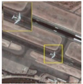 | 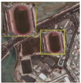 |
| SRGAN * | 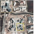 |  | 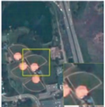 | 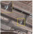 | 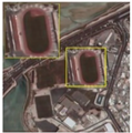 |
| ESRGAN | 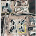 |  | 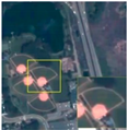 |  | 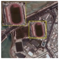 |
| ESRGAN * | 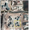 | 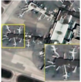 | 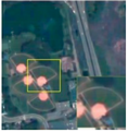 | 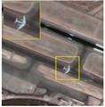 | 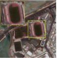 |
| MCWESRGAN | 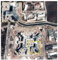 |  | 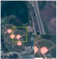 | 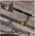 |  |
| MCWESRGAN * | 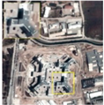 |  | 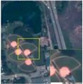 | 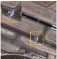 | 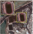 |
| Ground truth | 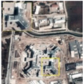 | 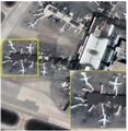 |  |  |  |
Appendix B
Table A2.
Quality assessment of convolutional network models dedicated to SISR for images with Appendix A. The best results are marked in green and the worst in red. “*” marks the SISR models with added Uformer network layers.
Table A2.
Quality assessment of convolutional network models dedicated to SISR for images with Appendix A. The best results are marked in green and the worst in red. “*” marks the SISR models with added Uformer network layers.
| Image 1 | ||||||||||||||||||
| Metric | EDSR | EDSR * | ESPCN | ESPCN * | FSRCNN | FSRCNN * | RDN | RDN * | SRCNN | SRCNN * | SRDenseNet | SRDenseNet * | SRGAN | SRGAN * | ESRGAN | ESRGAN * | MCWESRGAN | MCWESRGAN * |
| SSIM | 0.84 | 0.88 | 0.92 | 0.94 | 0.92 | 0.93 | 0.94 | 0.94 | 0.89 | 0.92 | 0.94 | 0.94 | 0.74 | 0.83 | 0.84 | 0.87 | 0.94 | 0.96 |
| PSNR | 26.36 | 27.2 | 31.26 | 27.16 | 30.88 | 32.37 | 32.99 | 32.79 | 29.0 | 30.65 | 32.88 | 32.64 | 22.56 | 24.57 | 26.96 | 28.15 | 33.02 | 34.08 |
| SAM | 0.09 | 0.08 | 0.05 | 0.08 | 0.05 | 0.04 | 0.04 | 0.04 | 0.06 | 0.05 | 0.04 | 0.04 | 0.13 | 0.11 | 0.08 | 0.07 | 0.04 | 0.03 |
| SCC | 0.34 | 0.43 | 0.42 | 0.25 | 0.32 | 0.41 | 0.44 | 0.43 | 0.32 | 0.43 | 0.40 | 0.42 | 0.11 | 0.28 | 0.26 | 0.38 | 0.45 | 0.46 |
| UQI | 0.99 | 0.99 | 1.0 | 0.97 | 1.00 | 1.00 | 1.00 | 1.00 | 1.00 | 1.00 | 1.00 | 1.00 | 0.98 | 0.99 | 0.99 | 1.00 | 1.00 | 1.00 |
| Image 2 | ||||||||||||||||||
| SSIM | 0.85 | 0.89 | 0.93 | 0.94 | 0.93 | 0.94 | 0.95 | 0.94 | 0.91 | 0.93 | 0.94 | 0.94 | 0.78 | 0.86 | 0.86 | 0.88 | 0.95 | 0.96 |
| PSNR | 25.26 | 25.77 | 29.78 | 30.01 | 29.93 | 31.08 | 31.34 | 31.41 | 27.85 | 29.15 | 30.91 | 31.12 | 22.8 | 24.57 | 26.02 | 27.36 | 31.68 | 32.46 |
| SAM | 0.10 | 0.09 | 0.06 | 0.06 | 0.06 | 0.05 | 0.05 | 0.05 | 0.07 | 0.06 | 0.05 | 0.05 | 0.13 | 0.10 | 0.09 | 0.07 | 0.05 | 0.04 |
| SCC | 0.25 | 0.31 | 0.30 | 0.31 | 0.22 | 0.29 | 0.30 | 0.30 | 0.23 | 0.29 | 0.27 | 0.29 | 0.09 | 0.21 | 0.19 | 0.25 | 0.31 | 0.32 |
| UQI | 0.99 | 0.99 | 1.00 | 1.00 | 1.00 | 1.00 | 1.00 | 1.00 | 1.00 | 1.00 | 1.00 | 1.00 | 0.98 | 0.99 | 0.99 | 0.99 | 1.00 | 1.00 |
| Image 3 | ||||||||||||||||||
| SSIM | 0.93 | 0.95 | 0.98 | 0.97 | 0.97 | 0.97 | 0.97 | 0.97 | 0.96 | 0.97 | 0.98 | 0.97 | 0.85 | 0.92 | 0.92 | 0.94 | 0.98 | 0.98 |
| PSNR | 32.26 | 33.9 | 38.35 | 37.57 | 35.93 | 37.2 | 37.01 | 37.01 | 34.34 | 36.37 | 38.35 | 37.36 | 23.86 | 25.4 | 30.88 | 31.79 | 37.67 | 37.41 |
| SAM | 0.06 | 0.05 | 0.03 | 0.03 | 0.04 | 0.04 | 0.04 | 0.04 | 0.05 | 0.04 | 0.03 | 0.03 | 0.15 | 0.12 | 0.07 | 0.07 | 0.03 | 0.03 |
| SCC | 0.17 | 0.22 | 0.20 | 0.20 | 0.13 | 0.19 | 0.18 | 0.18 | 0.14 | 0.21 | 0.17 | 0.19 | 0.05 | 0.16 | 0.11 | 0.16 | 0.19 | 0.20 |
| UQI | 1.00 | 1.00 | 1.00 | 1.00 | 1.00 | 1.00 | 1.00 | 1.00 | 1.00 | 1.00 | 1.00 | 1.00 | 0.97 | 0.97 | 0.99 | 0.99 | 1.00 | 1.00 |
| Image 4 | ||||||||||||||||||
| SSIM | 0.92 | 0.95 | 0.98 | 0.98 | 0.96 | 0.97 | 0.97 | 0.98 | 0.96 | 0.97 | 0.98 | 0.98 | 0.87 | 0.93 | 0.91 | 0.94 | 0.98 | 0.98 |
| PSNR | 31.68 | 33.13 | 38.58 | 39.62 | 35.79 | 38.58 | 38.02 | 39.46 | 34.31 | 37.77 | 39.41 | 39.44 | 26.54 | 28.98 | 32.0 | 34.52 | 39.29 | 40.17 |
| SAM | 0.06 | 0.05 | 0.02 | 0.02 | 0.03 | 0.02 | 0.03 | 0.02 | 0.04 | 0.03 | 0.02 | 0.02 | 0.1 | 0.07 | 0.05 | 0.04 | 0.02 | 0.02 |
| SCC | 0.22 | 0.31 | 0.28 | 0.28 | 0.18 | 0.26 | 0.28 | 0.29 | 0.22 | 0.29 | 0.26 | 0.28 | 0.09 | 0.23 | 0.14 | 0.24 | 0.30 | 0.30 |
| UQI | 1.00 | 1.00 | 1.00 | 1.00 | 1.00 | 1.00 | 1.00 | 1.00 | 1.00 | 1.00 | 1.00 | 1.00 | 0.99 | 0.99 | 1.00 | 1.00 | 1.00 | 1.00 |
| Image 5 | ||||||||||||||||||
| SSIM | 0.89 | 0.92 | 0.95 | 0.95 | 0.95 | 0.96 | 0.96 | 0.96 | 0.93 | 0.95 | 0.96 | 0.96 | 0.82 | 0.89 | 0.88 | 0.90 | 0.96 | 0.98 |
| PSNR | 28.99 | 29.89 | 34.23 | 34.59 | 33.62 | 35.14 | 35.65 | 35.46 | 31.87 | 33.25 | 35.67 | 35.25 | 24.77 | 26.96 | 29.73 | 30.89 | 35.87 | 36.94 |
| SAM | 0.09 | 0.08 | 0.05 | 0.05 | 0.05 | 0.04 | 0.04 | 0.04 | 0.06 | 0.05 | 0.04 | 0.04 | 0.14 | 0.11 | 0.08 | 0.07 | 0.04 | 0.03 |
| SCC | 0.26 | 0.34 | 0.31 | 0.33 | 0.25 | 0.32 | 0.34 | 0.33 | 0.26 | 0.33 | 0.31 | 0.32 | 0.09 | 0.24 | 0.18 | 0.28 | 0.34 | 0.36 |
| UQI | 0.99 | 1.00 | 1.00 | 1.00 | 1.00 | 1.00 | 1.00 | 1.00 | 1.00 | 1.00 | 1.00 | 1.00 | 0.99 | 0.99 | 1.00 | 1.00 | 1.00 | 1.00 |
References
- Rujoiu-Mare, M.-R.; Mihai, B.-A. Mapping Land Cover Using Remote Sensing Data and GIS Techniques: A Case Study of Prahova Subcarpathians. Procedia Environ. Sci. 2016, 32, 244–255. [Google Scholar] [CrossRef]
- Hejmanowska, B.; Kramarczyk, P.; Głowienka, E.; Mikrut, S. Reliable Crops Classification Using Limited Number of Sentinel-2 and Sentinel-1 Images. Remote Sens. 2021, 13, 3176. [Google Scholar] [CrossRef]
- Han, P.; Huang, J.; Li, R.; Wang, L.; Hu, Y.; Wang, J.; Huang, W. Monitoring Trends in Light Pollution in China Based on Nighttime Satellite Imagery. Remote Sens. 2014, 6, 5541–5558. [Google Scholar] [CrossRef]
- Hall, O.; Hay, G.J. A Multiscale Object-Specific Approach to Digital Change Detection. Int. J. Appl. Earth Obs. Geoinf. 2003, 4, 311–327. [Google Scholar] [CrossRef]
- Nasiri, V.; Hawryło, P.; Janiec, P.; Socha, J. Comparing Object-Based and Pixel-Based Machine Learning Models for Tree-Cutting Detection with PlanetScope Satellite Images: Exploring Model Generalization. Int. J. Appl. Earth Obs. Geoinf. 2023, 125, 103555. [Google Scholar] [CrossRef]
- Li, W.; Zhou, J.; Li, X.; Cao, Y.; Jin, G. Few-Shot Object Detection on Aerial Imagery via Deep Metric Learning and Knowledge Inheritance. Int. J. Appl. Earth Obs. Geoinf. 2023, 122, 103s397. [Google Scholar] [CrossRef]
- Stateczny, A.; Kazimierski, W.; Gronska-Sledz, D.; Motyl, W. The Empirical Application of Automotive 3D Radar Sensor for Target Detection for an Autonomous Surface Vehicle’s Navigation. Remote Sens. 2019, 11, 1156. [Google Scholar] [CrossRef]
- de Moura, N.V.A.; de Carvalho, O.L.F.; Gomes, R.A.T.; Guimarães, R.F.; de Carvalho Júnior, O.A. Deep-Water Oil-Spill Monitoring and Recurrence Analysis in the Brazilian Territory Using Sentinel-1 Time Series and Deep Learning. Int. J. Appl. Earth Obs. Geoinf. 2022, 107, 102695. [Google Scholar] [CrossRef]
- Greidanus, H. Satellite Imaging for Maritime Surveillance of the European Seas. In Remote Sensing of the European Seas; Barale, V., Gade, M., Eds.; Springer: Dordrecht, The Netherlands, 2008; pp. 343–358. ISBN 978-1-4020-6772-3. [Google Scholar]
- Gavankar, N.L.; Ghosh, S.K. Automatic Building Footprint Extraction from High-Resolution Satellite Image Using Mathematical Morphology. Eur. J. Remote Sens. 2018, 51, 182–193. [Google Scholar] [CrossRef]
- Reda, K.; Kedzierski, M. Detection, Classification and Boundary Regularization of Buildings in Satellite Imagery Using Faster Edge Region Convolutional Neural Networks. Remote Sens. 2020, 12, 2240. [Google Scholar] [CrossRef]
- d’Angelo, P.; Máttyus, G.; Reinartz, P. Skybox Image and Video Product Evaluation. Int. J. Image Data Fusion 2016, 7, 3–18. [Google Scholar] [CrossRef]
- Yang, T.; Wang, X.; Yao, B.; Li, J.; Zhang, Y.; He, Z.; Duan, W. Small Moving Vehicle Detection in a Satellite Video of an Urban Area. Sensors 2016, 16, 1528. [Google Scholar] [CrossRef] [PubMed]
- Kawulok, M.; Tarasiewicz, T.; Nalepa, J.; Tyrna, D.; Kostrzewa, D. Deep Learning for Multiple-Image Super-Resolution of Sentinel-2 Data. In Proceedings of the 2021 IEEE International Geoscience and Remote Sensing Symposium IGARSS, Brussels, Belgium, 11–16 July 2021; pp. 3885–3888. [Google Scholar]
- Dong, H.; Supratak, A.; Mai, L.; Liu, F.; Oehmichen, A.; Yu, S.; Guo, Y. TensorLayer: A Versatile Library for Efficient Deep Learning Development. In Proceedings of the 25th ACM International Conference on Multimedia, Mountain View, CA, USA, 23–27 October 2017; pp. 1201–1204. [Google Scholar]
- Goodfellow, I.J.; Pouget-Abadie, J.; Mirza, M.; Xu, B.; Warde-Farley, D.; Ozair, S.; Courville, A.; Bengio, Y. Generative Adversarial Networks. arXiv 2014, arXiv:1406.2661. [Google Scholar] [CrossRef]
- Kim, J.; Lee, J.K.; Lee, K.M. Accurate Image Super-Resolution Using Very Deep Convolutional Networks. In Proceedings of the 2016 IEEE Conference on Computer Vision and Pattern Recognition (CVPR), Las Vegas, NV, USA, 27–30 June 2016; pp. 1646–1654. [Google Scholar]
- Fu, J.; Liu, Y.; Li, F. Single Frame Super Resolution with Convolutional Neural Network for Remote Sensing Imagery. In Proceedings of the IGARSS 2018—2018 IEEE International Geoscience and Remote Sensing Symposium, Valencia, Spain, 22–27 July 2018; pp. 8014–8017. [Google Scholar]
- Lanaras, C.; Bioucas-Dias, J.; Galliani, S.; Baltsavias, E.; Schindler, K. Super-Resolution of Sentinel-2 Images: Learning a Globally Applicable Deep Neural Network. ISPRS J. Photogramm. Remote Sens. 2018, 146, 305–319. [Google Scholar] [CrossRef]
- Lim, B.; Son, S.; Kim, H.; Nah, S.; Lee, K.M. Enhanced Deep Residual Networks for Single Image Super-Resolution. In Proceedings of the 2017 IEEE Conference on Computer Vision and Pattern Recognition Workshops (CVPRW), Honolulu, HI, USA, 21–26 July 2017; pp. 1132–1140. [Google Scholar]
- Pouliot, D.; Latifovic, R.; Pasher, J.; Duffe, J. Landsat Super-Resolution Enhancement Using Convolution Neural Networks and Sentinel-2 for Training. Remote Sens. 2018, 10, 394. [Google Scholar] [CrossRef]
- Xiao, A.; Wang, Z.; Wang, L.; Ren, Y. Super-Resolution for “Jilin-1” Satellite Video Imagery via a Convolutional Network. Sensors 2018, 18, 1194. [Google Scholar] [CrossRef] [PubMed]
- Wang, Y.; Fevig, R.; Schultz, R.R. Super-Resolution Mosaicking of UAV Surveillance Video. In Proceedings of the 2008 15th IEEE International Conference on Image Processing, San Diego, CA, USA, 12–15 October 2008; pp. 345–348. [Google Scholar]
- Demirel, H.; Anbarjafari, G. IMAGE Resolution Enhancement by Using Discrete and Stationary Wavelet Decomposition. IEEE Trans. Image Process. 2011, 20, 1458–1460. [Google Scholar] [CrossRef] [PubMed]
- Dong, W.; Zhang, L.; Shi, G.; Wu, X. Nonlocal Back-Projection for Adaptive Image Enlargement. In Proceedings of the 2009 16th IEEE International Conference on Image Processing (ICIP), Cairo, Egypt, 7–10 November 2009; pp. 349–352. [Google Scholar]
- Dong, C.; Loy, C.C.; Tang, X. Accelerating the Super-Resolution Convolutional Neural Network. In Computer Vision—ECCV 2016; Leibe, B., Matas, J., Sebe, N., Welling, M., Eds.; Springer International Publishing: Cham, Switzerland, 2016; pp. 391–407. [Google Scholar]
- Haris, M.; Shakhnarovich, G.; Ukita, N. Deep Back-Projection Networks for Super-Resolution. In Proceedings of the 2018 IEEE/CVF Conference on Computer Vision and Pattern Recognition, Salt Lake City, UT, USA, 18–23 June 2018; pp. 1664–1673. [Google Scholar]
- Xiao, Y.; Yuan, Q.; He, J.; Zhang, Q.; Sun, J.; Su, X.; Wu, J.; Zhang, L. Space-Time Super-Resolution for Satellite Video: A Joint Framework Based on Multi-Scale Spatial-Temporal Transformer. Int. J. Appl. Earth Obs. Geoinf. 2022, 108, 102731. [Google Scholar] [CrossRef]
- Choi, Y.-J.; Kim, B.-G. HiRN: Hierarchical Recurrent Neural Network for Video Super-Resolution (VSR) Using Two-Stage Feature Evolution. Appl. Soft Comput. 2023, 143, 110422. [Google Scholar] [CrossRef]
- Wang, P.; Sertel, E. Multi-Frame Super-Resolution of Remote Sensing Images Using Attention-Based GAN Models. Knowl. Based Syst. 2023, 266, 110387. [Google Scholar] [CrossRef]
- Jin, X.; He, J.; Xiao, Y.; Yuan, Q. Learning a Local-Global Alignment Network for Satellite Video Super-Resolution. IEEE Geosci. Remote Sens. Lett. 2023, 20, 1–5. [Google Scholar] [CrossRef]
- Liu, H.; Gu, Y.; Wang, T.; Li, S. Satellite Video Super-Resolution Based on Adaptively Spatiotemporal Neighbors and Nonlocal Similarity Regularization. IEEE Trans. Geosci. Remote Sens. 2020, 58, 8372–8383. [Google Scholar] [CrossRef]
- He, Z.; Li, X.; Qu, R. Video Satellite Imagery Super-Resolution via Model-Based Deep Neural Networks. Remote Sens. 2022, 14, 749. [Google Scholar] [CrossRef]
- Li, S.; Sun, X.; Gu, Y.; Lv, Y.; Zhao, M.; Zhou, Z.; Guo, W.; Sun, Y.; Wang, H.; Yang, J. Recent Advances in Intelligent Processing of Satellite Video: Challenges, Methods, and Applications. IEEE J. Sel. Top. Appl. Earth Obs. Remote Sens. 2023, 16, 6776–6798. [Google Scholar] [CrossRef]
- Yin, Q.; Hu, Q.; Liu, H.; Zhang, F.; Wang, Y.; Lin, Z.; An, W.; Guo, Y. Detecting and Tracking Small and Dense Moving Objects in Satellite Videos: A Benchmark. IEEE Trans. Geosci. Remote Sens. 2022, 60, 1–18. [Google Scholar] [CrossRef]
- Zhao, M.; Li, S.; Xuan, S.; Kou, L.; Gong, S.; Zhou, Z. SatSOT: A Benchmark Dataset for Satellite Video Single Object Tracking. IEEE Trans. Geosci. Remote Sens. 2022, 60, 1–11. [Google Scholar] [CrossRef]
- He, Q.; Sun, X.; Yan, Z.; Li, B.; Fu, K. Multi-Object Tracking in Satellite Videos With Graph-Based Multitask Modeling. IEEE Trans. Geosci. Remote Sens. 2022, 60, 1–13. [Google Scholar] [CrossRef]
- Xiao, Y.; Su, X.; Yuan, Q.; Liu, D.; Shen, H.; Zhang, L. Satellite Video Super-Resolution via Multiscale Deformable Convolution Alignment and Temporal Grouping Projection. IEEE Trans. Geosci. Remote Sens. 2022, 60, 1–19. [Google Scholar] [CrossRef]
- Wang, X.; Sun, L.; Chehri, A.; Song, Y. A Review of GAN-Based Super-Resolution Reconstruction for Optical Remote Sensing Images. Remote Sens. 2023, 15, 5062. [Google Scholar] [CrossRef]
- Karwowska, K.; Wierzbicki, D. Using Super-Resolution Algorithms for Small Satellite Imagery: A Systematic Review. IEEE J. Sel. Top. Appl. Earth Obs. Remote Sens. 2022, 15, 3292–3312. [Google Scholar] [CrossRef]
- Wang, X.; Liu, Y.; Zhang, H.; Fang, L. A Total Variation Model Based on Edge Adaptive Guiding Function for Remote Sensing Image De-Noising. Int. J. Appl. Earth Obs. Geoinf. 2015, 34, 89–95. [Google Scholar] [CrossRef]
- Irum, I.; Sharif, M.; Raza, M.; Mohsin, S. A Nonlinear Hybrid Filter for Salt & Pepper Noise Removal from Color Images. J. Appl. Res. Technology. JART 2015, 13, 79–85. [Google Scholar] [CrossRef]
- Wang, B.; Ma, Y.; Zhang, J.; Zhang, H.; Zhu, H.; Leng, Z.; Zhang, X.; Cui, A. A Noise Removal Algorithm Based on Adaptive Elevation Difference Thresholding for ICESat-2 Photon-Counting Data. Int. J. Appl. Earth Obs. Geoinf. 2023, 117, 103207. [Google Scholar] [CrossRef]
- Yang, H.; Su, X.; Wu, J.; Chen, S. Non-Blind Image Blur Removal Method Based on a Bayesian Hierarchical Model with Hyperparameter Priors. Optik 2020, 204, 164178. [Google Scholar] [CrossRef]
- Wang, Z.; Cun, X.; Bao, J.; Zhou, W.; Liu, J.; Li, H. Uformer: A General U-Shaped Transformer for Image Restoration. In Proceedings of the 2022 IEEE/CVF Conference on Computer Vision and Pattern Recognition (CVPR), New Orleans, LA, USA, 18–24 June 2022; pp. 17662–17672. [Google Scholar]
- Shen, Z.; Wang, W.; Lu, X.; Shen, J.; Ling, H.; Xu, T.; Shao, L. Human-Aware Motion Deblurring. In Proceedings of the 2019 IEEE/CVF International Conference on Computer Vision (ICCV), Seoul, Republic of Korea, 27 October–2 November 2019; pp. 5571–5580. [Google Scholar]
- Rim, J.; Lee, H.; Won, J.; Cho, S. Real-World Blur Dataset for Learning and Benchmarking Deblurring Algorithms. In Computer Vision—ECCV 2020; Vedaldi, A., Bischof, H., Brox, T., Frahm, J.-M., Eds.; Springer International Publishing: Cham, Switzerland, 2020; pp. 184–201. [Google Scholar]
- Nah, S.; Kim, T.H.; Lee, K.M. Deep Multi-Scale Convolutional Neural Network for Dynamic Scene Deblurring. In Proceedings of the IEEE Conference on Computer Vision and Pattern Recognition, Honolulu, HI, USA, 21–26 July 2017; pp. 257–265. [Google Scholar]
- Kupyn, O.; Budzan, V.; Mykhailych, M.; Mishkin, D.; Matas, J. DeblurGAN: Blind Motion Deblurring Using Conditional Adversarial Networks. In Proceedings of the 2018 IEEE/CVF Conference on Computer Vision and Pattern Recognition, Salt Lake City, UT, USA, 18–23 June 2018; pp. 8183–8192. [Google Scholar]
- Xu, L.; Zheng, S.; Jia, J. Unnatural L0 Sparse Representation for Natural Image Deblurring. In Proceedings of the 2013 IEEE Conference on Computer Vision and Pattern Recognition, Portland, OR, USA, 23–28 June 2013; pp. 1107–1114. [Google Scholar]
- Kupyn, O.; Martyniuk, T.; Wu, J.; Wang, Z. DeblurGAN-v2: Deblurring (Orders-of-Magnitude) Faster and Better. In Proceedings of the 2019 IEEE/CVF International Conference on Computer Vision (ICCV), Seoul, Republic of Korea, 27–28 October 2019; pp. 8877–8886. [Google Scholar]
- Zhang, K.; Luo, W.; Zhong, Y.; Ma, L.; Stenger, B.; Liu, W.; Li, H. Deblurring by Realistic Blurring. In Proceedings of the 2020 IEEE/CVF Conference on Computer Vision and Pattern Recognition (CVPR), Seattle, WA, USA, 13–19 June 2020; pp. 2734–2743. [Google Scholar]
- Purohit, K.; Suin, M.; Rajagopalan, A.N.; Boddeti, V.N. Spatially-Adaptive Image Restoration Using Distortion-Guided Networks. In Proceedings of the IEEE/CVF International Conference on Computer Vision, Montreal, BC, Canada, 11–17 October 2021; pp. 2309–2319. [Google Scholar]
- Zhang, J.; Pan, J.; Ren, J.; Song, Y.; Bao, L.; Lau, R.W.H.; Yang, M.-H. Dynamic Scene Deblurring Using Spatially Variant Recurrent Neural Networks. In Proceedings of the 2018 IEEE/CVF Conference on Computer Vision and Pattern Recognition, Salt Lake City, UT, USA, 18–23 June 2018; pp. 2521–2529. [Google Scholar]
- Tao, X.; Gao, H.; Shen, X.; Wang, J.; Jia, J. Scale-Recurrent Network for Deep Image Deblurring. In Proceedings of the 2018 IEEE/CVF Conference on Computer Vision and Pattern Recognition, Salt Lake City, UT, USA, 18–23 June 2018; pp. 8174–8182. [Google Scholar]
- Zhang, H.; Dai, Y.; Li, H.; Koniusz, P. Deep Stacked Hierarchical Multi-Patch Network for Image Deblurring. In Proceedings of the IEEE/CVF Conference on Computer Vision and Pattern Recognition, Long Beach, CA, USA, 15–20 June 2019; pp. 5978–5986. [Google Scholar]
- Zamir, S.W.; Arora, A.; Khan, S.; Hayat, M.; Khan, F.S.; Yang, M.-H.; Shao, L. Multi-Stage Progressive Image Restoration. In Proceedings of the 2021 IEEE/CVF Conference on Computer Vision and Pattern Recognition (CVPR), Nashville, TN, USA, 20–25 June 2021; pp. 14816–14826. [Google Scholar]
- Karwowska, K.; Wierzbicki, D. MCWESRGAN: Improving Enhanced Super-Resolution Generative Adversarial Network for Satellite Images. IEEE J. Sel. Top. Appl. Earth Obs. Remote Sens. 2023, 16, 9459–9479. [Google Scholar] [CrossRef]
- Richardson, W.H. Bayesian-Based Iterative Method of Image Restoration. J. Opt. Soc. Am. 1972, 62, 55–59. [Google Scholar] [CrossRef]
- Orieux, F.; Giovannelli, J.-F.; Rodet, T. Bayesian Estimation of Regularization and PSF Parameters for Wiener-Hunt Deconvolution. J. Opt. Soc. Am. A 2010, 27, 1593–1607. [Google Scholar] [CrossRef] [PubMed]
- Karwowska, K.; Wierzbicki, D. Improving Spatial Resolution of Satellite Imagery Using Generative Adversarial Networks and Window Functions. Remote Sens. 2022, 14, 6285. [Google Scholar] [CrossRef]
- Wang, X.; Yu, K.; Wu, S.; Gu, J.; Liu, Y.; Dong, C.; Qiao, Y.; Loy, C.C. ESRGAN: Enhanced Super-Resolution Generative Adversarial Networks. In Computer Vision—ECCV 2018 Workshops; Leal-Taixé, L., Roth, S., Eds.; Springer International Publishing: Cham, Switzerland, 2019; pp. 63–79. [Google Scholar]
- Kantorovich, L.V.; Rubinshtein, S.G. On a Space of Totally Additive Functions. Vestn. St. Petersburg Univ. Math. 1958, 13, 52–59. [Google Scholar]
- Wang, D.; Liu, Q. Learning to Draw Samples: With Application to Amortized MLE for Generative Adversarial Learning. arXiv 2016, arXiv:1611.01722. [Google Scholar]
- Charbonnier, P.; Blanc-Feraud, L.; Aubert, G.; Barlaud, M. Two Deterministic Half-Quadratic Regularization Algorithms for Computed Imaging. In Proceedings of the 1st International Conference on Image Processing, Austin, TX, USA, 13–16 November 1994; Volume 2, pp. 168–172. [Google Scholar]
- Zamir, S.W.; Arora, A.; Khan, S.; Hayat, M.; Khan, F.S.; Yang, M.-H.; Shao, L. Learning Enriched Features for Real Image Restoration and Enhancement. arXiv 2020, arXiv:1611.01722. [Google Scholar]
- Keelan, B. Handbook of Image Quality: Characterization and Prediction; CRC Press: Boca Raton, FL, USA, 2002; ISBN 978-0-429-22280-1. [Google Scholar]
- Wang, Z.; Bovik, A.C. A Universal Image Quality Index. IEEE Signal Process. Lett. 2002, 9, 81–84. [Google Scholar] [CrossRef]
- Goetz, A.; Boardman, W.; Yunas, R. Discrimination among Semi-Arid Landscape Endmembers Using the Spectral Angle Mapper (SAM) Algorithm. JPL, Summaries of the Third Annual JPL Airborne Geoscience Workshop. Volume 1: AVIRIS Workshop. 1992. Available online: https://ntrs.nasa.gov/search.jsp?R=19940012238 (accessed on 24 November 2023).
- Xia, G.-S.; Bai, X.; Ding, J.; Zhu, Z.; Belongie, S.; Luo, J.; Datcu, M.; Pelillo, M.; Zhang, L. DOTA: A Large-Scale Dataset for Object Detection in Aerial Images. In Proceedings of the IEEE Conference on Computer Vision and Pattern Recognition, Salt Lake City, UT, USA, 18–23 June 2018; pp. 3974–3983. [Google Scholar]
- Chang Guang Satellite Technology Co., Ltd. Available online: http://www.jl1.cn/EWeb/ (accessed on 24 November 2023).
- Planet|Homepage. Available online: https://www.planet.com/ (accessed on 24 November 2023).


Disclaimer/Publisher’s Note: The statements, opinions and data contained in all publications are solely those of the individual author(s) and contributor(s) and not of MDPI and/or the editor(s). MDPI and/or the editor(s) disclaim responsibility for any injury to people or property resulting from any ideas, methods, instructions or products referred to in the content. |
© 2024 by the authors. Licensee MDPI, Basel, Switzerland. This article is an open access article distributed under the terms and conditions of the Creative Commons Attribution (CC BY) license (https://creativecommons.org/licenses/by/4.0/).