Abstract
This article presents a method within a Bayesian framework for quantifying uncertainty in satellite aerosol remote sensing when retrieving aerosol optical depth (AOD). By using a Bayesian model averaging technique, we take into account uncertainty in aerosol optical model selection and also obtain a shared inference about AOD based on the best-fitting optical models. In particular, uncertainty caused by forward-model approximations has been taken into account in the AOD retrieval process to obtain a more realistic uncertainty estimate. We evaluated a model discrepancy, i.e., forward-model uncertainty, empirically by exploiting the residuals of model fits and using a Gaussian process to characterise the discrepancy. We illustrate the method with examples using observations from the TROPOspheric Monitoring Instrument (TROPOMI) on the Sentinel-5 Precursor satellite. We evaluated the results against ground-based remote sensing aerosol data from the Aerosol Robotic Network (AERONET).
1. Introduction
Remote sensing of atmospheric aerosols by satellite instruments provides a global as well as locally focused view of the distribution of aerosols. Aerosol retrieval algorithms are continuously improved to meet the needs of different user groups in the fields of climate and air quality monitoring. It is essential to include uncertainty estimates in the retrieved aerosol information in order to utilise the results properly, e.g., in assimilation applications into numerical models or in air quality modelling. An overview of the uncertainty and its assessment in satellite remote sensing is provided in [1]. The satellite aerosol products include quality flags, which provide information to the data user about the potential failure of the retrieved pixel. In addition, formal error propagation methods, such as the optimal estimation method, also provide an estimate of the total retrieval uncertainty in their results. A statistical approach is relevant when analysing the uncertainty originating from assumptions and approximations made in the retrieval method or from modelling of the physical system. Sayer et al. [2] discuss diagnostic and prognostic (i.e., predictive) approaches for uncertainty quantification in the satellite aerosol retrievals. That article details different approaches to obtain pixel-level aerosol optical depth (AOD) uncertainty estimates in aerosol retrieval algorithms and also proposes a framework for evaluating the uncertainty estimates. The retrieval quality study by [3] presents model-enforced post-processing which uses machine learning techniques for correcting inaccuracies in the results of a satellite aerosol product. Overall, research focusing on uncertainty analysis and improvement of the uncertainty estimate benefits both the retrieval algorithm developers and data users.
In this article, we present a statistical method for retrieving AOD with associated uncertainty estimates and apply it to the TROPOspheric Monitoring Instrument (TROPOMI) on board the Copernicus Sentinel-5 Precursor (S5P) satellite. The TROPOMI instrument provides daily global observations used for monitoring atmospheric composition. TROPOMI radiance measurements are processed into data products, which include aerosol index, aerosol layer height, carbon monoxide, formaldehyde, methane, nitrogen dioxide, sulphur dioxide, ozone, surface UV and cloud properties. These data products are used for various applications, such as aviation safety, air quality services, and monitoring of CO and NO2 emissions [4].
Currently, there are two operational TROPOMI aerosol products which are the ultraviolet (UV) aerosol index product and the aerosol layer height product. Both of the products have been developed by the Royal Netherlands Meteorological Institute (KNMI). The TROPOMI UV aerosol index product consists of two retrievals, one for wavelength pair 340/380 nm and the other for 354/388 nm [5,6]. The UV aerosol index product is suitable for monitoring the development and dispersion of aerosol plumes, e.g., from wildfires, dust storms and volcanic ash eruptions, since it also works in the presence of clouds. The TROPOMI aerosol layer height product provides the height of the free-tropospheric aerosol layer in cloudless situations [7]. Additionally, NASA’s aerosol algorithm TROPOMAER retrieves the aerosol UV index, aerosol absorption optical depth, total aerosol optical depth, aerosol layer height and aerosol single-scattering albedo (SSA) using TROPOMI near-ultraviolet radiances [8]. The Generalized Retrieval of Aerosol and Surface Properties (GRASP) is an algorithm for the characterisation of aerosol and surface properties from satellite and surface measurements. The GRASP algorithm has been applied to TROPOMI observations to obtain, e.g., AOD, Ångström exponent and SSA (https://www.grasp-open.com/products/ (accessed on 20 May 2024)). Rao et al. [9] present a study using synthetic and real TROPOMI measurements from the O2 A band (758–771 nm) to retrieve both AOD level and aerosol layer height. Their algorithm is based on the selection of microphysical aerosol models, and the results showed that, when there is difficulty in selecting the proper aerosol model, the accuracy of the solution increases if one applies a Bayesian approach.
Our quantity of interest is the AOD at a reference wavelength of 500 nm. It is retrieved using top-of-atmosphere (TOA) radiances across a broad wavelength range in the UV–visible (UVIS) and near-infrared (NIR) spectra. AOD is a measure of aerosol vertical loading but does not unambiguously indicate the aerosol type or its origin. In satellite aerosol retrieval, a forward model is computed using an atmospheric radiative transfer (RT) model, which can be a very complex system. Additionally, when RT is performed simultaneously with the retrieval inversion, the computational cost can become high. For this reason, many operational satellite algorithms are based on pre-calculated forward-model simulations whose results are stored in look-up tables (LUTs). In the inversion, forward-model computations are carried out by interpolating LUTs. We also use the LUT-based retrieval approach in this study. The retrieval methodology is based on Bayesian inference for model selection and model averaging. We use a similar statistical approach to that employed in previous studies for the Ozone Monitoring Instrument (OMI) on board NASA’s Earth Observing System (EOS) Aura satellite [10]. In addition to this work, we have created multi-dimensional LUTs using the RT model from the libRadtran software package (e.g., [11,12]). The RT model simulates the TROPOMI signals in various atmospheric aerosol states. Each LUT contains an aerosol optical model consisting of aerosol microphysical (e.g., particle size, complex refractive index and particle shape) and optical properties (e.g., SSA and scattering matrices) for a particular type of aerosol at different AOD levels and sun–satellite geometries. Then, in the actual retrieval process, the optical models are matched to the TOA satellite observations, and AOD estimates and aerosol type are obtained at the same time. The advantage of the LUT-based retrieval is that it allows one to look at the ability of the method to select the proper aerosol optical models, as well as being able to obtain new information about the model selection process. Specifically, we have included some dust-type models with a non-spherical particle shape which represent new types of models in this context.
In this study, we focus on uncertainty related to aerosol optical model selection (see, e.g., [13,14]) and, consequently, the effect of the selected model on the retrieved AOD. We also note the uncertainty due to forward modelling in the retrieval process, as the forward model is only an approximation of the real forward function. This forward-model uncertainty is referred to as model discrepancy (or forward-model uncertainty) [15,16]. The model discrepancy is characterised using a Gaussian process model. An estimate for the model discrepancy term was obtained through an empirical approach based on smooth systematic differences between the TROPOMI-measured reflectance and the LUT-based forward-modelled reflectance. This task was performed in advance before starting the actual AOD retrieval process.
We describe in Section 2 the satellite data and databases used. We give the aerosol type definitions and describe the construction of the LUTs using radiative transfer calculations (see also Appendix A). We present a statistical methodology for uncertainty quantification when retrieving AOD and associated aerosol types. Finally, in Section 3, we demonstrate the method with case studies. In Section 4, we give a summary and draw conclusions from this study.
2. Materials and Methods
2.1. TROPOMI/S5P Observations
The Copernicus Sentinel-5P is a collaborative mission between the European Commissions, the European Space Agency (ESA) and the Netherlands Space Office. The S5P satellite carrying the TROPOMI instrument was launched on 13 October 2017. It is a polar-orbiting satellite on a sun-synchronous orbit with an equatorial crossing time at ∼13:30 solar time. TROPOMI measures in the wavelength range between 270 and 2358 nm including ultraviolet, visible, near-infrared and shortwave infrared wavelength bands. TROPOMI has a high spatial resolution as the size of the ground pixel at nadir can be as small as 5.5 × 3.5 km2, but the pixel size ultimately depends on the data product.
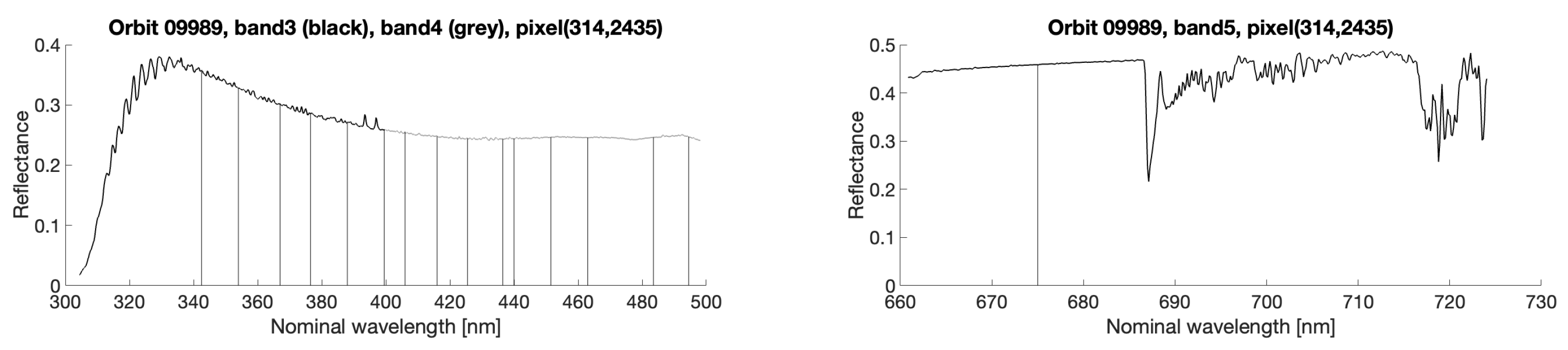
We computed the reflectance from the TROPOMI radiance and irradiance spectrum. We selected the level 1b irradiance file that has the sensing time closest to the level 1b radiance’s sensing time. In this study we use 16 wavelength bands from the TROPOMI UVIS (spectral bands 3 and 4) and NIR (spectral band 5) detectors. The ∼1 nm wide wavelength bands are centred at 342.5, 354.0, 367.0, 376.5, 388.0 and 399.5 nm (from band 3); 406.0, 416.0, 425.5, 436.5, 440.0, 451.5, 463.0, 483.5 and 494.5 nm (from band 4), and 675.0 nm (from band 5). Our unknown AOD is retrieved at the reference wavelength 500 nm. The wavelength bands selected are relatively evenly distributed across the total wavelength range. In Figure 1, the TROPOMI reflectance spectrum in one pixel is shown for detector bands 3 and 4 (left-hand panel) and for band 5 (right-hand panel), respectively. The wavelengths used in the retrieval process have been denoted by vertical lines. The main reason for including these wavelength bands is that, except for 440 nm and 675 nm, they have already been evaluated for the multi-wavelength OMI aerosol algorithm (see [17]). Additionally, we included bands 440 nm and 675 nm because AOD from the AErosol RObotic NETwork (AERONET) are provided at these wavelengths.

Figure 1.
The TROPOMI reflectance spectrum for example pixel. Vertical lines show the 16 wavelength bands used in the range of band 3 (black) and band 4 (grey) (left), and in the range of band 5 (right), respectively.
We obtained latitude and longitude coordinates assigned to the centre of the ground pixel from the level 1b band 3 radiance file. Since we only deal with small pixel sets in the case studies (Section 3), actual cloud screening was not carried out. The following quality checks were performed on the TROPOMI ground pixels before being used in the case studies. First, we checked the ’ground_pixel_quality’ value from the level 1b band 3 radiance data file and omitted the pixel if its value differed from zero [18]. Additionally, the solar zenith angle (SZA) must not exceed 75°. We also assessed the pixel quality by utilising the quality flag variable ’qa_value’ from the TROPOMI level 2 UV aerosol index product. We rejected the pixel if the ’qa_value’ was less than 0.5 [19].
2.2. AERONET
AERONET is a federation of ground-based aerosol networks (see [20], https://aeronet.gsfc.nasa.gov (accessed on 20 May 2024)). The results of the case studies (Section 3) have been evaluated against ground-based remote sensing aerosol data from the collocated AERONET sites (see Table 1). We downloaded Version 3 direct-sun, cloud-screened and quality-controlled AOD data from AERONET (e.g., [21]). Additionally, the AERONET Version 3 inversion product provides aerosol type information, for example the size distribution and refractive index (e.g., [22,23]), which is useful in evaluating the results.

Table 1.
The collocated AERONET sites and the results of the case studies. The column AOD (500) AERONET contains the average of the AOD at 500 nm values measured within a one-hour time window coinciding with the TROPOMI overpass time. The column AOD S5P contains the MAP AOD estimate from the averaged posterior density.
2.3. Aerosol Model Properties and Creation of the Look-Up Tables
The LUTs are multi-dimensional tables constructed by radiative transfer runs for different sun–satellite geometries and for various aerosol properties. Generally speaking, the use of LUTs in the satellite retrieval algorithms is justified since it reduces the computational costs. In the retrieval process, the LUTs are typically evaluated by interpolation. In this study, the LUTs containing optical models are classified by the main aerosol types: weakly absorbing (WA), biomass burning (BB) and desert dust (DD) aerosols (see Section 2.3.1). The aerosol characteristics (e.g., size distribution and absorption coefficients) are provided as input when running the forward radiative transfer (RT) model (see Section 2.3.2).
2.3.1. Aerosol Types
The main aerosol types, i.e., WA, BB and DD, are split into subtypes according to the size distribution and absorption properties of the aerosol particles. We have a total of 66 optical models to use when applying the method for solving the inverse problem. More precisely, we have altogether nine WA models, 27 BB models and 30 DD models in the collection of LUTs. We would like to point out that the range of aerosol optical and microphysical properties considered is specific to our study and is not intended to encompass a comprehensive collection of aerosol mixtures. For example, sea salt and volcanic ash aerosol models are not included. Additional information on the aerosol properties and the assignment of model identification numbers (IDs) can be found in Appendix A.
The classification is made based on an origin of the aerosols. The aerosols classified as weakly absorbing aerosols originate from urban, industrial and rural sources. The class of biomass burning includes smoke aerosols originating from, e.g., natural sources such as wildfires. The chemical composition of the BB type aerosols may consist of black carbon or organic carbon. Additionally, vehicle emissions and combustion processes in an urban or industrial environment can be a source of soot. There are different types of dust with dissimilar mineralogy from arid and semi-arid regions, e.g., the Sahara, Asia, Sahel, the Middle East, Australia and South America. The dust particles have, depending on their origin, different mineralogical compositions and therefore different scattering and absorption properties.
2.3.2. Radiative Transfer Simulation for FORWARD Model
The forward-model computations with radiative transfer have been carried out in advance as preliminary preparation for the actual retrieval process. The RT simulations are performed by the RT software package libRadtran (version 2.0.3) (e.g., [11,12]), which is a library of radiative transfer tools and programs. We have used the DISORT 2.0 and MYSTIC solvers for the radiative transfer. LibRadtran’s main input data are the wavelength range, atmospheric model and aerosol optical characteristics. Furthermore, among other things, an observational geometry of the instrument is provided as input data. We have applied the U.S. 1976 standard atmosphere for a vertical profile of the atmosphere. As input to the libRadtran are given the aerosol optical properties, including a phase matrix, SSA and an Ångström exponent. Therefore, the aerosol microphysical properties (i.e., size distribution, refractive index and particle shape) have been converted to the optical properties using the Modelled Optical Properties of enSeMbles of Aerosol Particles (MOPSMAP) tool. The MOPSMAP tool includes a Fortran program to perform computations on a personal computer and a web interface for interactive use. The basic principle is that the tool calculates the optical properties of the aerosol particles by interpolating in a MOPSMAP grid of particle sizes, shapes and refractive indices. More information about the MOPSMAP tool can be found in the user manual at https://mopsmap.net/mopsmap_userguide.pdf (accessed on 20 May 2024) and in the article [24]. The output from the libRadtran run are the atmospheric reflectance , the transmittance T and the spherical albedo s (see Table 2). These values are stored in the LUT together with the associated instrument geometry and the aerosol microphysical properties.
Table 2.
The LUT variables obtained from the RT simulations. These variables are used to calculate the modelled TOA reflectance in Equation (2).
2.4. Methodology Description
We denote by symbol = our unknown parameter AOD at a reference wavelength = 500 nm. We utilise Bayesian statistical inference (see, e.g., [25]) in the retrieval and consider an unknown AOD as a random variable. The solution is expressed as a posterior density of AOD. A width of the posterior density describes a level of uncertainty. However, in order to provide some point estimate we use a maximum a posteriori (MAP) estimate of AOD, i.e., a mode of the posterior density. The MAP estimate is a single AOD value that maximises the posterior probability. In some case the posterior may have many peaks, i.e., the posterior is multi-modal. In such a case, we usually choose the highest mode as the MAP estimate. The point estimate is often used when the retrieved AOD is assessed by comparing it with reference data, e.g., AOD measured by Sun photometers from stations that are part of the AERONET.
The basic principle is that the solution is sought through aerosol model selection. In the retrieval process, we choose the optical models that are most plausible in explaining the satellite-measured spectral reflectance. Here, the aerosol optical model is a discrete atmospheric characterisation with certain aerosol type and different aerosol loads. The LUTs containing aerosol optical models have been created beforehand with radiative transfer simulations using assumptions and approximations of reality (see Section 2.3.2). In this work, we acknowledge this uncertainty due to imperfect forward modelling. The model discrepancy (i.e., forward-model uncertainty) has been estimated by exploiting residuals of model fits, as described in Section 2.5.
The observation model, that maps the atmospheric state to the measured spectra, is given as
where is the measured TOA spectral reflectance, is the forward-model-based reflectance, is our quantity of interest and is the vector of wavelength bands. The model discrepancy is at the centre of this work (see Section 2.5) and appears as additional uncertainty in the observation model. The model discrepancy comprises uncertainty related to, e.g., input parameters for forward model run, optical model selection, LUT interpolation and surface reflectance assumption. The term is the measurement error due to instrument noise and it is assumed to be independent and zero-mean Gaussian . Since this is a research-type retrieval algorithm, for simplicity, we have set , and used a constant value for a signal-to-noise ratio (SNR) of the instrument. As a rough estimate, we used the value SNR = 700 when applying the methodology in the case studies presented in Section 3. We would like to point out that, while in this work we ended up with a value of SNR = 700, the SNR value can be adjusted to reflect the true TROPOMI signal in further work.
In this work, we process only over-land pixels. Therefore, we can use the following formula (e.g., [26]) to calculate the forward model, i.e., the modelled TOA reflectance:
where is a surface reflectance, is a path reflectance, T is a transmittance and s is a spherical albedo of the atmosphere as seen from below. The values for , T and s are taken from the LUT (see Table 2) by interpolating within node points. These nodal parameters are (AOD), (a cosine of viewing zenith angle), (a cosine of solar zenith angle), (a relative azimuth angle) and (a surface pressure). The values at the nodal points have been calculated using the radiative transfer model (see Section 2.3.2).
The surface reflectance is included in the forward model via Equation (2). We have taken the values from the surface reflectance database for ESA’s earth observation missions (ADAM) (https://earth.esa.int/eogateway/catalog/adam-surface-reflectance-database-v4-0 (accessed on 20 May 2024)). The ADAM product includes a global climatology map of monthly mean values of the surface reflectance at 0.1° spatial resolution for land. The ADAM database provides surface reflectance dependent on the instrument’s viewing direction.
2.5. Model Discrepancy Estimation
In practice, we look at systematic differences between the modelled and observed reflectance, and use them to estimate the model discrepancy. We have utilised a Gaussian process approach [15,27] to characterise the model discrepancy. Similar approach was used when applied to the OMI measurements and is described in detail in [10]. We apply a Gaussian process model GP with zero mean and the covariance function C. The covariance C is characterised by a wavelength-dependent systematic structure in the residuals of model fits . Basically, we are inspecting spectral correlation of the residuals. The spectral dependence is described by a (semi)variogram function, which is approximated here by an empirical semivariance. The empirical semivariance is calculated at each wavelength pair distance as
where is the number of wavelength pairs with the distance d. Section 2.1 lists the wavelength bands used here except for the NIR wavelength band 675.0 nm which we omitted. The band 675.0 nm has such a long distance to the other UV and VIS wavelength bands (see Figure 1) that a spectral correlation is not presumed. The empirical semivariance as a function of distance d between wavelengths is depicted in Figure 2a.
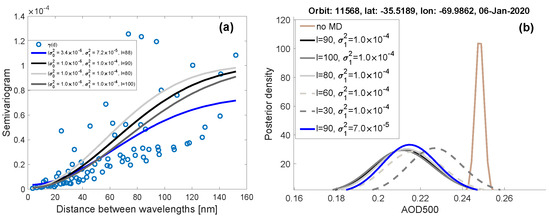
Figure 2.
(a) The theoretical Gaussian semivariogram model with different values for tuning parameters , and correlation length l (solid curves) is fitted to the empirical semivariogram (circles). (b) The resulting posteriors corresponding to the different parameter values for and l. Also, the resulting posterior when the model discrepancy was not included (identified as no MD in the Figure legend) is shown.
Next, we choose a theoretical parametric double exponential (i.e., Gaussian) variogram model from the literature (e.g., [28]):
where . A correlation length describes the wavelength distance where the residuals are still correlated. Additionally, the parameter (i.e., nugget) is responsible for a non-spectral diagonal variance and the parameter for a spectral variance. We obtain estimates for these tuning parameters l, and using the empirical semivariogram. Figure 2a shows the empirical semivariogram (circles) as well as the theoretical semivariogram model (solid curves) with different parameter values.
Based on the theoretical variogram model (e.g., [28]) we derive the covariance function C of the Gaussian process model as
This depends on the wavelength distance and determines the correlation properties of the model discrepancy. Eventually, the covariance function forms the corresponding model error covariance matrix that determines the allowed spectral departure of the forward-modelled reflectance from the observed reflectance. In this study, we used the parameter value as l = 90 nm, and for and we used the value of of the measured reflectance. This selection of parameter values closely corresponds to the black curve in Figure 2a which has l = 90, and . Figure 2b illustrates the sensitivity of the resulting posterior density of AOD to the different values for the covariance function parameters l and . We can observe that the posterior reflects the change in l and . For the sake of comparison, the posterior density when the model discrepancy was not taken into account is also plotted in Figure 2b. When the correlation length l decreases, the posterior approaches the posterior without model discrepancy, as may be expected.
In the experiment, the calculation of the residuals was conducted for the pixels collected on two separate days: 24 July 2019 and 22 March 2019. The modelled reflectance was interpolated from the model that best matched the measured reflectance in a least squares sense. For the residual analysis, a higher noise level (SNR = 300) was chosen. In this case, the requirement for fit between the measured and modelled reflectance is relaxed; otherwise, the number of successful retrievals would remain unnecessarily small. The pixel sets used in the residual calculation were collected from seven orbits that crossed all continents, thus ensuring worldwide distribution. The number of pixels processed was 2162 for 24 July and 617 for 22 March, respectively. The ratio of the number of successfully retrieved pixels to the number of pixels processed was ∼39% for 24 July and ∼12% for 22 March, respectively. The ensemble of residuals included can be considered a representative sample, since only 15 out of 66 optical models were never selected as the best model.
2.6. Bayesian Approach for Retrieving AOD
By Bayes’ theorem, the posterior distribution for after observing is
where we assume the model m is correct. We set the a priori distribution for within the model m to be a log-normal distribution (e.g., [29]), i.e., with a mean value and standard deviation . This is a conventional choice for a prior distribution for AOD as it makes the distribution wide with a large deviation. It is only weakly informative but ensures that can only obtain positive real values. We have used this same log-normal prior for each individual model that is matched to a measurement in case studies (Section 3). The likelihood function, which now includes a model error covariance matrix , is
The normalising constant in Equation (6) does not depend on . Since we have a one-dimensional problem, we can calculate the normalising constant numerically. Consequently, we can compute the full posterior in the retrieval process. Finally, we have as a solution an estimate for AOD with related uncertainty.
2.7. Aerosol Model Selection
In our approach, the aerosol optical model selection is executed by comparing probabilities of observing given the model m. Probability is called evidence for the model m. This probability has already been evaluated because it also acts as a normalising constant in Equation (6). We fit all the models, one by one, and select those models which have the highest evidence values. That is, the best models are identified according to their evidence values. We accept models based on the highest evidence values among the best-fitting models until the cumulative sum of the evidence values exceeds 0.8 or until the 10 best models have been selected.
Next, we will present how to compare the selected best-fitting models with each other and rank them in order of suitability. We use Bayes’ theorem again to obtain the posterior of a model m conditional to the measurement
where is a prior probability that the model m explains the measurement. We can also note that the evidence term occurs as a likelihood in Equation (8). We have a priori assumption that all the optical models are equally likely, i.e., . This means that we use no pre-selected models for a single retrieval pixel according to a land cover type or climatology for instance. In this case, Equation (8) for the model obtains a simple format
where the denominator is the sum over the evidence values of all the selected models. This is a formula for the relative evidence for model and it can be used for comparison of the models based on their evidence values. Thus, we can conclude that the higher the relative evidence the more plausible the aerosol model is to explain the measurement.
2.8. Bayesian Model Averaging
We combine the posterior densities of for the selected models using the Bayesian model averaging technique [30]:
where n is the number of the selected best models. The model’s relative evidence (Equation (9)) acts here as a weight. Thus, we obtain the shared inference about based on the several best models. In addition, the averaged posterior reflects uncertainty in the aerosol model selection. When the distinct models yield different (i.e., AOD estimates) the uncertainty in the averaged posterior may be larger than the uncertainty in any single model. In order to compare the result directly with reference values, e.g., AOD from satellite products or AOD from the ground-based AERONET, we need a point estimate. We have chosen the MAP estimate from the averaged posterior to be the point estimate for .
2.9. Goodness of Fit
However, the fact that we have selected the best models does not yet guarantee acceptance of the solution. Therefore, we check whether the selected model with the highest evidence fits the measurement sufficiently. To check the goodness of fit, we calculate a modified chi-squared value over the n wavelength bands as
where we have included the model error covariance matrix . We used acceptance criterion for the solution as ≤ 2. The reason for rejecting the solution is that none of the models fit well enough for the measurement. This may be due to cloud contamination or because an appropriate model is missing from the collection of LUTs.
3. Results
As a result, we obtained the AOD estimate from the averaged posterior density. Additionally, we retrieved information about the aerosol type based on the most probable aerosol optical models. The point estimate for AOD was set to be the MAP AOD estimate from the averaged posterior density.
The results of the case studies were evaluated against ground-based remote sensing aerosol data from the collocated AERONET sites. In Table 1 are listed the AERONET sites involved and the collocated TROPOMI pixels together with the AOD values. We used a simple geometric collocation criterion such that we took a TROPOMI pixel for which a solution was retrieved and whose centre coordinates were closest to the coordinates of the AERONET site. As a temporal collocation criterion we used a rule that we included those AERONET AOD (500 nm) values that were measured within a one-hour time window coinciding with the TROPOMI overpass time.
3.1. Case South America: Transported Smoke from Australian Bush Fires in January 2020
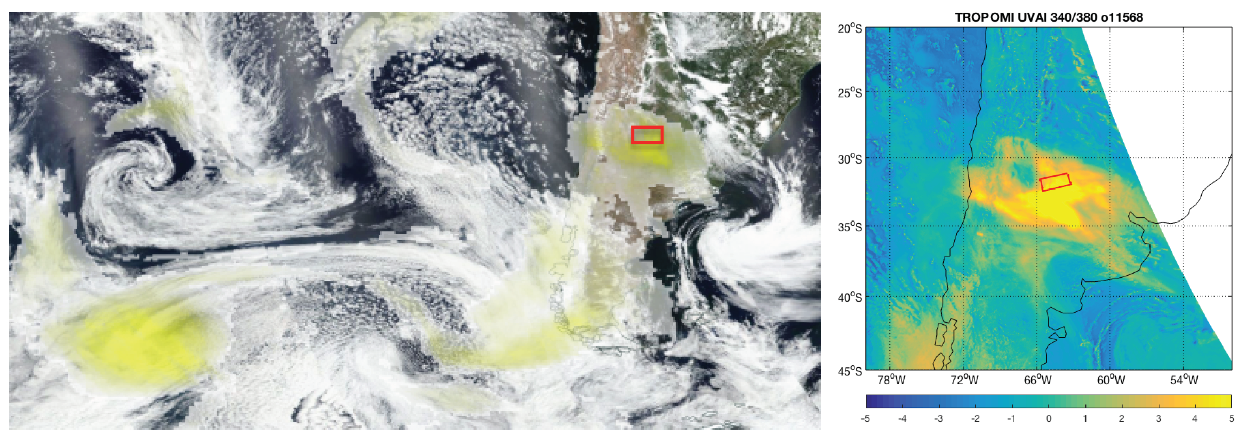
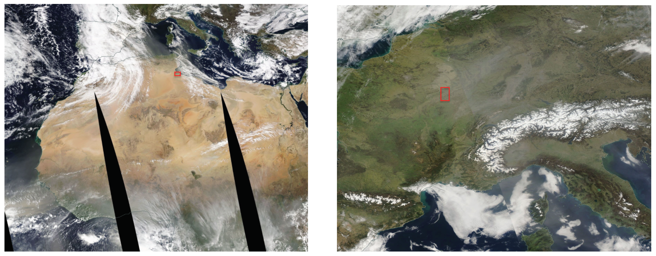
This case study examines the detection of smoke aerosols in South America on 6 January 2020 emitted from bush fires in Australia. Devastating wildfires occurred in various parts of Australia, continuing for about nine months during the 2019–2020 season. Figure 3 (left-hand panel) illustrates the transported aerosol plume over the Pacific Ocean on 6 January 2020. Yellow colour indicates elevated levels of the aerosol index due to smoke from fires in Australia. This image is provided by the EOSDIS Worldview tool as part of a story showcasing satellite images related to the Australian bushfires (https://worldview.earthdata.nasa.gov (accessed on 20 May 2024)). An elevated amount of absorbing aerosols can also be detected in Figure 3 (right-hand panel) from the operational TROPOMI UV aerosol index product (wavelength pair 340/380 nm). Positive values indicate the presence of UV-absorbing aerosols, while near-zero and negative values indicate the presence of clouds and non-absorbing aerosols [5]. The area studied is marked with a “red” rectangle in the images.
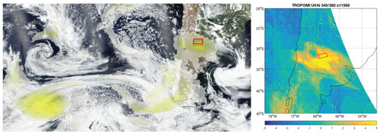
Figure 3.
On 6 January 2020 smoke aerosols transported from Australia to South America. The EOSDIS Worldview combined image of Visible Infrared Imaging Radiometer Suite (VIIRS) reflectance (true-colour) and aerosol index from the Ozone Mapping and Profiler Suite (OMPS) onboard the joint NASA/NOAA Suomi NPP satellite (left). The aerosol index from the TROPOMI UV aerosol index product (340/380 nm) (right). A red rectangle marks the area examined.
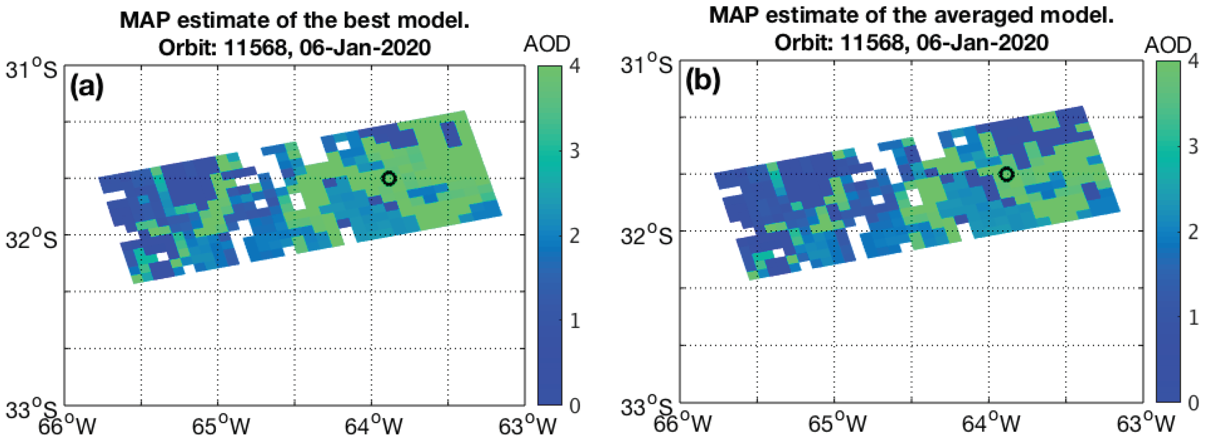
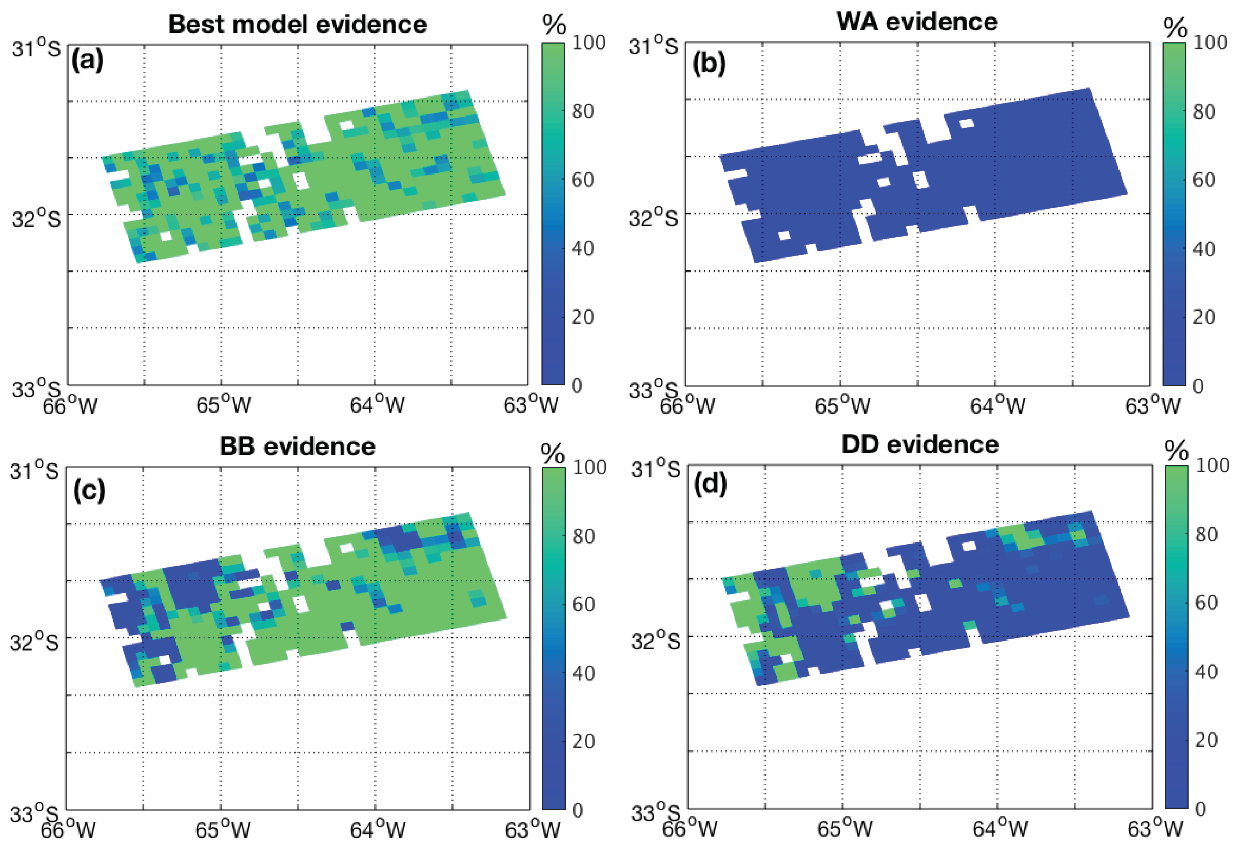
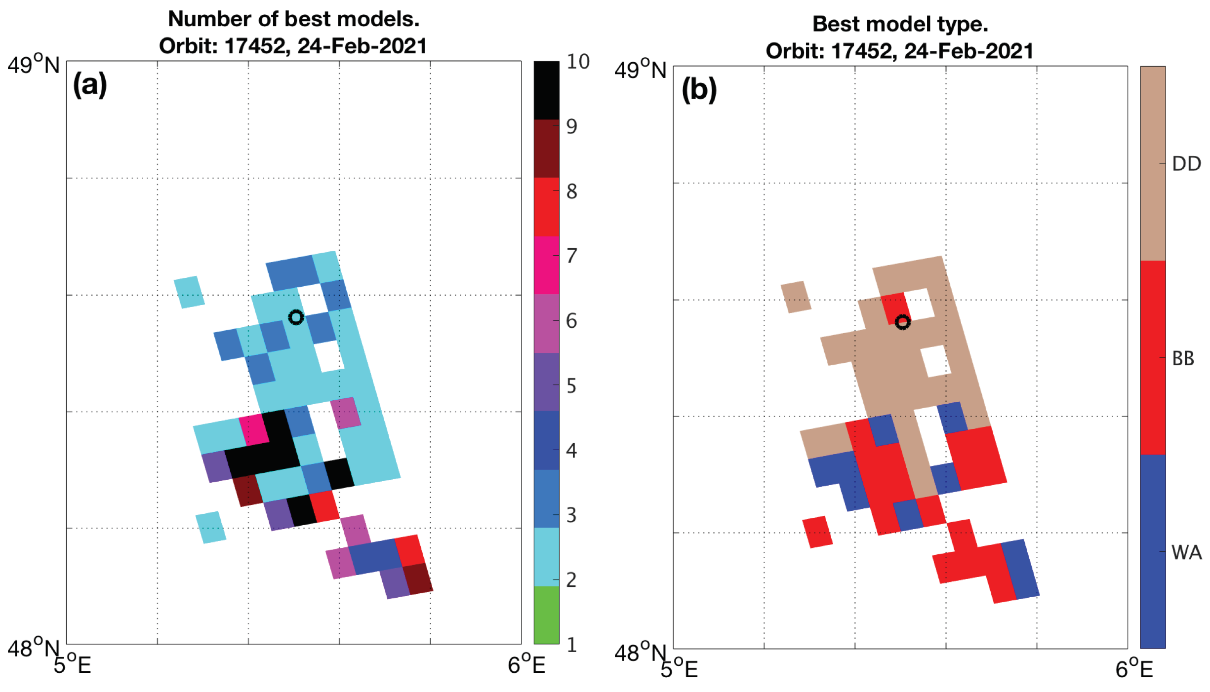
Figure 4 shows the retrieved MAP AOD estimates from the single best model (a) and from the averaged posterior density (b), respectively. The pixel is empty if the solution has not been obtained, i.e., none of the models fit well enough for the observation. A black circle displayed on the pixel grid shows the location of the AERONET station Pilar_Cordoba. As can be seen, we retrieve very high AOD levels (that is, values above 2) around this AERONET site. We can conclude from Figure 4 with caution that, if the MAP AOD estimate is based on one model, it produces higher AOD values than if a MAP AOD estimate is derived from the averaged posterior that combines best-fitting models. However, for the majority of the retrieval pixels, only one or two aerosol models were chosen as can be seen from Figure 5a. This can also be inferred from Figure 6a showing each pixel the relative evidence of the most likely model. That is, if one model is enough to explain the measurement, its relative evidence is 100%. The prevailing main aerosol type is biomass burning, as we can see in Figure 5b and Figure 6c. Nevertheless, DD aerosols and a mixture of BB and DD aerosols are also present for some pixels (see Figure 6c,d).
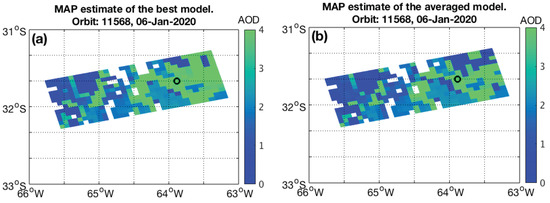
Figure 4.
On 6 January 2020, orbit: 11,568. (a) The MAP AOD estimate of the best model, that is, the model with the highest evidence. (b) The MAP AOD estimate from the averaged posterior, i.e., combination of the selected best models. The location of the AERONET site Pilar_Cordoba is marked with a black circle.
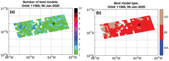
Figure 5.
On 6 January 2020, orbit: 11,568. (a) The spatial distribution of the number of the best models selected and (b) the main aerosol type of the best individual model with the highest evidence. The location of the AERONET site Pilar_Cordoba is marked with a black circle.
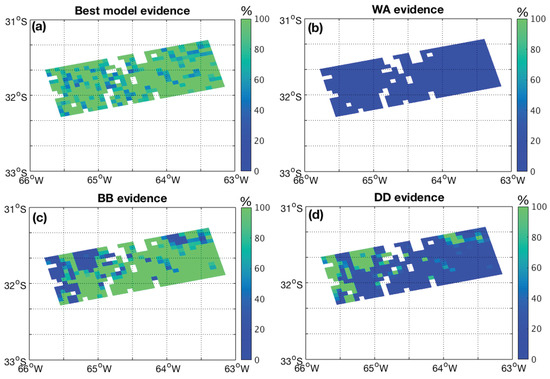
Figure 6.
On 6 January 2020, orbit: 11,568. The spatial distribution of the relative evidence (%). (a) The relative evidence (%) of the best individual model with the highest evidence. (b–d) The relative evidence (%) within each main aerosol type, i.e., including all the best models of that type.
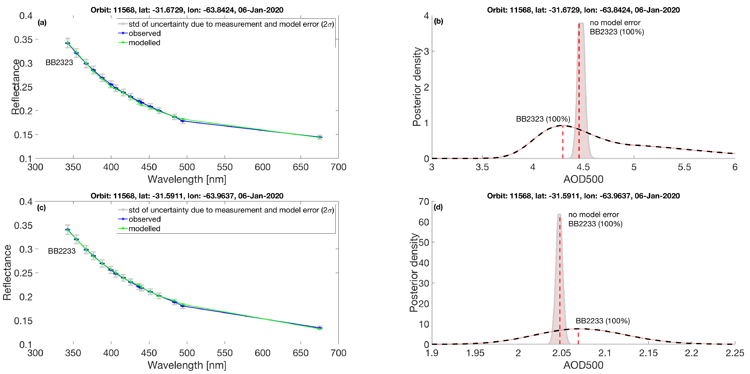
In Figure 7, the results are shown for the two pixels in the vicinity of the AERONET site Pilar_Cordoba. The measured reflectance (blue) and modelled reflectance (green) match well, as can be seen in Figure 7 (left-hand column). In the images displaying the posterior densities (right-hand column), the corresponding relative evidence (%) for each model is indicated next to its ID number (Equation (9)). For comparison, the resulting posterior densities are also displayed when the model discrepancy is not taken into account (filled curve). It is noticeable that, without accounting for the model discrepancy, we obtain a more optimistic uncertainty and a slightly different AOD estimate (a red vertical dashed line). The pixel (Figure 7a,b) closest to the Pilar_Cordoba site has a MAP AOD estimate of ∼4.3, which is much higher than the ground-based AOD (see Table 1). The other example pixel (Figure 7c,d), that is located a little bit further from the Pilar_Cordoba site, also has a high AOD (∼2). Please note that the measured reflectances do not differ much except at 675 nm (Figure 7a,c) but the obtained AOD estimates clearly differ from each other (Figure 7b,d). The reason for overestimating AOD compared to the AERONET results may be that the correct aerosol model is missing from our collection of LUTs. We refer to [31] that discusses strong spectral dependence in carbonaceous aerosol absorption in near-UV in the presence of organic carbon type biomass burning aerosols. It was found that overestimation of AOD at 500 nm occurs in the presence of organic carbon when absorption is assumed to be independent of wavelengths. This is the case in our biomass burning type of models with no wavelength dependence in absorption, i.e., the imaginary part of the refractive index is constant (Appendix A). The other reasons for overestimation of AOD could be surface reflectance effects or sub-pixel cloud contamination. As seen in Figure 3 (right panel) the UVAI values indicate the presence of UV-absorbing aerosols in the studied area. Therefore, we do not assume that cloud contamination is a reason for the overestimating AOD. Also, we can infer from AERONET data that there were absorbing aerosols in the air, since the spectral pattern of the imaginary part of the refractive index downloaded from the AERONET version 3 inversion product (https://aeronet.gsfc.nasa.gov (accessed on 20 May 2024) ) suggests the presence of absorbing organic carbon (i.e., brown carbon). However, it is noteworthy that the selected models, ’BB2323’ and ’BB2233’, place the aerosol layer at 2–4 km and 4–6 km in altitude, respectively (see Appendix A). This refers to a realistic operation of the aerosol model selection, as the transported smoke plume is presumably on the higher layer of the atmosphere (e.g., [32]).
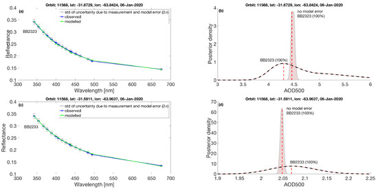
Figure 7.
On 6 January 2020, orbit: 11,568. The results are shown for the pixel indexed (394,1834) collocated to AERONET site Pilar_Cordoba (a,b) and for the pixel nearby it (393,1836) (c,d), respectively. The measured reflectance (blue dots) and the modelled reflectances (green dots) at the selected wavelength bands (left-hand column). The error bars (in grey) correspond to 2× standard measurement and forward-model error. The posterior density of AOD at 500 nm for each best-fitting model (right-hand column). The averaged posterior, based here on a single model, is shown on a black dashed curve. The resulting posterior, if the model discrepancy is not included (i.e., no model error), is displayed with a filled posterior curve (right). The MAP AOD estimate is indicated by a red vertical dashed line.
3.2. Desert Dust Cases
This case study examines the detection of Sahara dust aerosols in two different regions: near the source and further from the source. Snapshots of these two cases can be seen in true-colour Aqua/MODIS images from the EOSDIS Worldview tool (Figure 8). The areas studied are marked on the images with red rectangles. In the first case, 21 February 2021, a small area around the AERONET site Medenine_IRA in Tunisia is examined. The other case, 24 February 2021, examines whether the dust aerosols transported from the Sahara can be detected in Europe in the area around the AERONET site Bure_OPE in France.
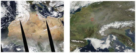
Figure 8.
True-colour Aqua/MODIS images taken from the EOSDIS Worldview tool, showing dust event in Northern Africa on 21 February 2021 (left) and dust passed into Europe on 24 February 2021 (right). The red rectangle marks the area examined.
Figure 9 shows the resulting MAP AOD estimates for 21 February 2021. The AERONET site Medenine_IRA is marked with a black circle in the image. We can notice elevated AOD values near Medenine_IRA and that the aerosol type is BB (see Figure 9, Figure 10b and Figure 11). In general, the prevailing type of aerosol is dust and, in some pixels, several DD models affect the retrieved AOD (see Figure 10 and Figure 11).
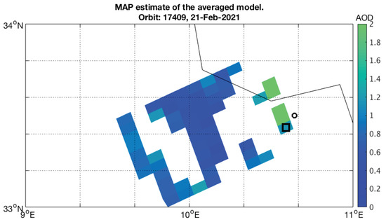
Figure 9.
On 21 February 2021, orbit: 17,409. The MAP AOD estimate from the averaged posterior. The location of the AERONET site Medenine_IRA is marked with a black circle. Since the solution is missing for that pixel we consider in more detail the nearby pixel indexed (60,2977) marked by a black rectangle (see Table 1 and Figure 12a,b).
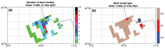
Figure 10.
On 21 February 2021, orbit: 17,409. For the dust case. (a) The spatial distribution of the number of the best models selected and (b) the main aerosol type of the best individual model with the highest evidence. The location of the AERONET site Medenine_IRA is marked with a black circle.
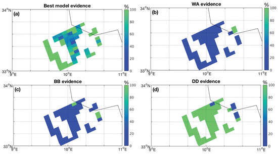
Figure 11.
On 21 February 2021, orbit: 17,409. The spatial distribution of the relative evidence (%). (a) The relative evidence (%) of the best individual model with the highest evidence. (b–d) The relative evidence (%) within each main aerosol type, i.e., including all the best models of that type.
Figure 12 displays the more detailed results for three pixels. The top pixel (first row) is the closest one to the AERONET site Medenine_IRA (marked in Figure 9). As a result, we obtain only one desert dust type of model. We can observe in Figure 12a that the modelled reflectance (green curve) does not agree so well with the observation (blue curve). The model discrepancy (see Equation (1)) allows a smooth departure from the modelled to the observed reflectance. If the model discrepancy was not included, there is no solution since the candidate models had too high a difference from the observed reflectance. The ground-based mean value AOD (500) ∼1.209 is comparable with the MAP AOD estimate ∼1.16 since it is within the uncertainty limits of the retrieved AOD (Figure 12b). Additionally, the mean value of the Ångström exponent (440–870 nm) is ∼0.091, as obtained from the AERONET site Medenine_IRA (https://aeronet.gsfc.nasa.gov (accessed on 20 May 2024)), indicating the presence of coarse particles. The Ångström exponent is a measure of the spectral dependence of AOD and usually it is inversely proportional to the effective particle size.
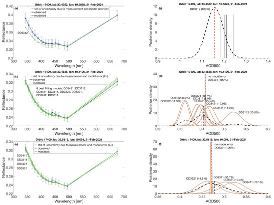
Figure 12.
On 21 February 2021, orbit: 17409. Same as Figure 7 but for the pixels near to AERONET site Medenine_IRA. Given more precisely, the TROPOMI pixels are (a,b) (60,2977), (c,d) (55,2981) and (e,f) (55,2982). The averaged posterior, based on the best-fitting models, is shown by a black dashed curve and the red vertical dashed line indicates the MAP AOD estimate from it. Gray vertical lines in (b) denote the AERONET AOD (500) values in a one-hour time window, including the TROPOMI overpass time, and the black vertical solid line is their average value.
For the other two pixels (Figure 12 middle and the bottom rows), there are a number of the DD type of model selected. Interestingly, the selected models represent both particle shapes, i.e., spherical (‘DD33xx’) and non-spherical (‘DD34xx’). The selected models also assume different heights of the aerosol layers as indicated by the third digit of the model ID number (see Appendix A). Then, we could conclude from the results that the mixture of dust aerosols is distributed at different heights. However, we must also consider the potential effects of surface reflectivity in this case. In Figure 12d, the averaged posterior (represented by the black dashed curve) exhibits more than one peak, indicating difficulty in the model selection process.
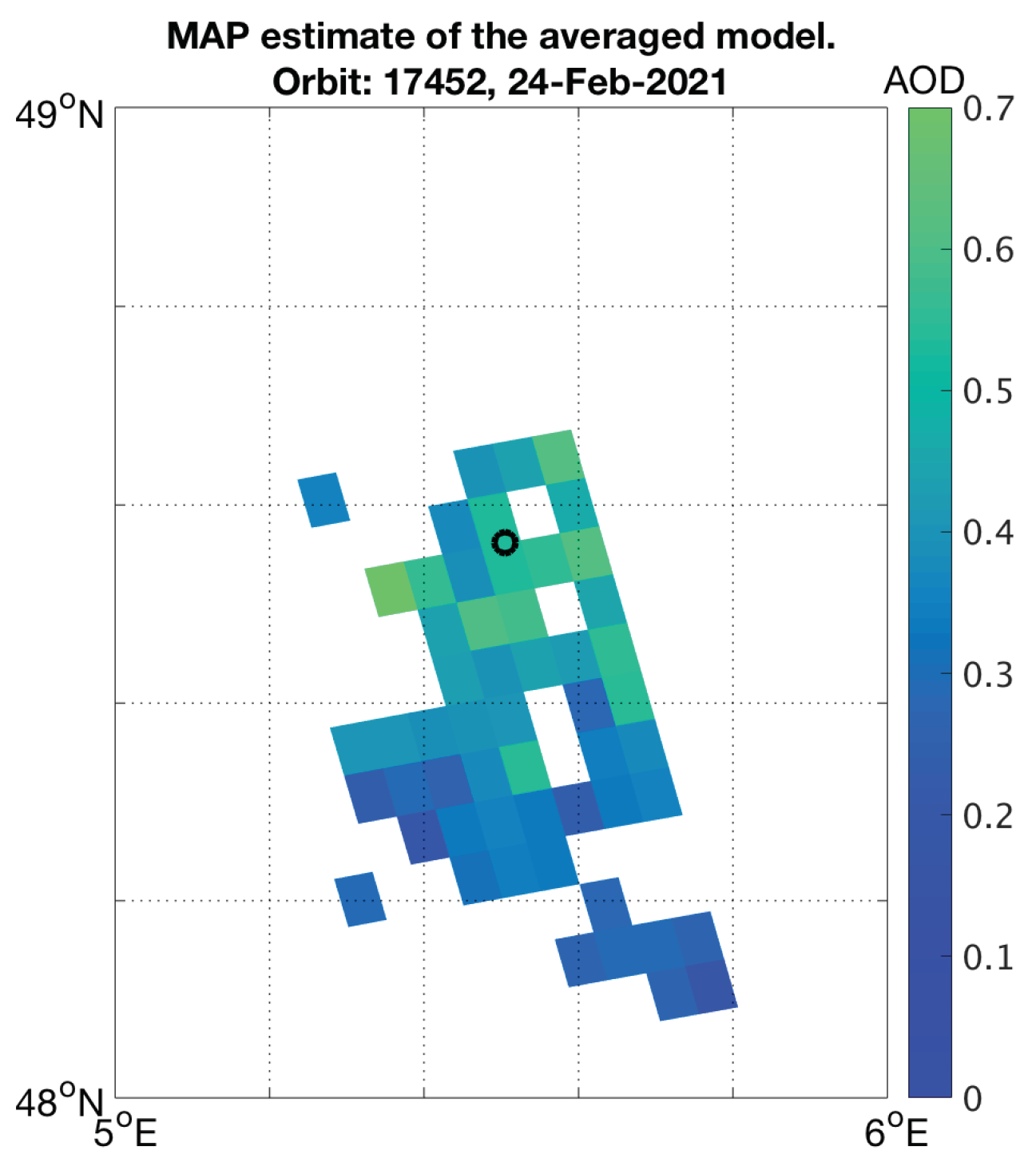
The second day (24 February 2021) deals with pixel area located in Europe. Figure 13 shows that there are elevated AOD levels in the vicinity of the AERONET site Bure_OPE. There are two TROPOMI pixels that are in collocation with the location of the Bure_OPE site. The resulting aerosol types for these two pixels are different; one is the biomass burning type and the other is the dust type (see Figure 14b). In Figure 14b and Figure 15d, it can be seen that there is an area where dust is the dominant aerosol type. On the other hand, there are pixels where we obtain as a result a mixture of several WA and BB types of model (see Figure 15). We can also detect that the AOD level is higher when the selected models are the dust type (see Figure 13, Figure 14 and Figure 15).
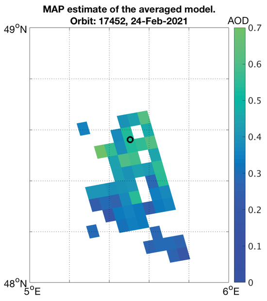
Figure 13.
On 4 February 2021, orbit: 17,452. Same as Figure 9. The location of the AERONET site Bure_OPE is marked with a black circle.

Figure 14.
On 24 February 2021, orbit: 17,452. Same as Figure 10 but for the case where dust has passed into Europe. (a) The spatial distribution of the number of the best models selected and (b) the main aerosol type of the best individual model with the highest evidence. The location of the AERONET site Bure_OPE is marked with a black circle.
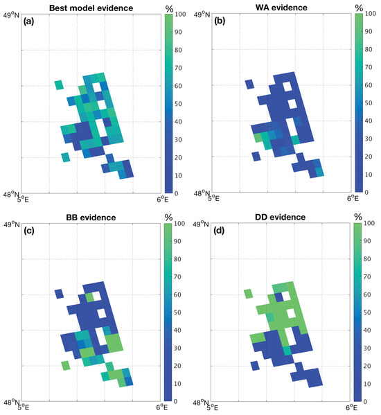
Figure 15.
On 24 February 2021, orbit: 17,452. Same as Figure 11 but for the case where dust has passed into Europe. The spatial distribution of the relative evidence (%). (a) The relative evidence (%) of the best individual model with the highest evidence. (b–d) The relative evidence (%) within each main aerosol type, i.e., including all the best models of that type.
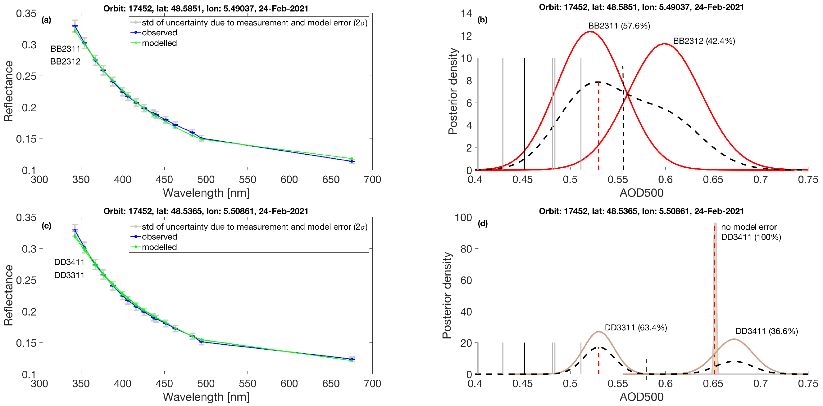
The detailed results for the two pixels collocated with the site Bure_OPE are shown in Figure 16. We can note that for both pixels the modelled reflectance matches the observed reflectance (left-hand column). Also, for both pixels, the resulting MAP AOD estimate is ∼0.53 and it is rather well comparable with the ground-based mean AOD value (∼0.45) from the Bure_OPE site (see Table 1). The upper row pixel (Figure 16a,b) has two BB models (‘BB2311’ and ‘BB2312’) as a result, and these models differ in size distribution (see Appendix A). When the model discrepancy has not been considered, a suitable model is not found. For the other pixel (Figure 16c,d), we obtain as a result two of the DD type of model, ‘DD3311’ (spherical) and ‘DD3411’ (non-spherical). These models differ only in terms of the shape of the particle. The difference in the retrieved AOD between these two shapes originates from the differences in the optical properties of the models (see Appendix A). As pointed out by the comparison of these two dust models ‘DD3311’ and ‘DD3411’ (see Figure A1), the differences are particularly large at smaller wavelengths (in the UV) and concern specifically the angular distribution of scattered intensity and the fraction of scattered light compared to extinction. In particular, the former will result in different estimates depending on the geometry of the satellite retrieval (i.e., the SZA and viewing zenith angle). The averaged posterior (black dashed curve) has two separate peaks (Figure 16d) that suggest that there are two distinct potential solutions. Since the model ‘DD3311’ has higher relative evidence (63.4%), the averaged posterior has a higher peak for that model, and consequently determines the retrieved AOD estimate indicated by the red dashed vertical line. On the other hand, if the model discrepancy was not accounted for (see the filled posterior in (d)), the best-fitting model is ‘DD3411’ (non-spherical).
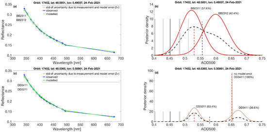
Figure 16.
On 24 February 2021, orbit: 17,452. The results are shown for the pixels (274,3205) (a,b) and (274,3204) (c,d) collocated to AERONET site Bure_OPE. The averaged posterior is shown on a black dashed curve. The red vertical dashed line stands for the MAP AOD estimate from the averaged posterior, whereas the black vertical dashed line indicates the weighted mean of the MAP AOD estimates from the individual posteriors. The gray vertical lines in (b,d) denote the AERONET AOD (500) values within a one-hour time window, including the TROPOMI overpass time, and the black vertical solid line is their average value.
By comparison, we also display a point value of AOD derived by , where the weight is the model relative evidence and is the MAP AOD estimates of the posterior. This weighted mean of the MAP AOD estimates is shown in Figure 16 (right-hand column) on a black vertical dashed line. For instance, in Figure 16b, we can note a small difference between the MAP AOD from the averaged posterior (∼0.53) and the weighted mean of the MAP AOD estimates (∼0.56), but the MAP AOD estimate from the averaged posterior is closer to the ground-based mean value AOD (∼0.45). According to the AERONET data at the Bure_OPE site, there were coarse particles (i.e., possibly dust particles) present since the reported daily mean value of the Ångström exponent (440–870 nm) for 24 February 2021 is 0.193, whereas the monthly average of the Ångström exponent for February 2021 is 1.017, normally indicating the presence of finer particles such as urban–industrial aerosols.
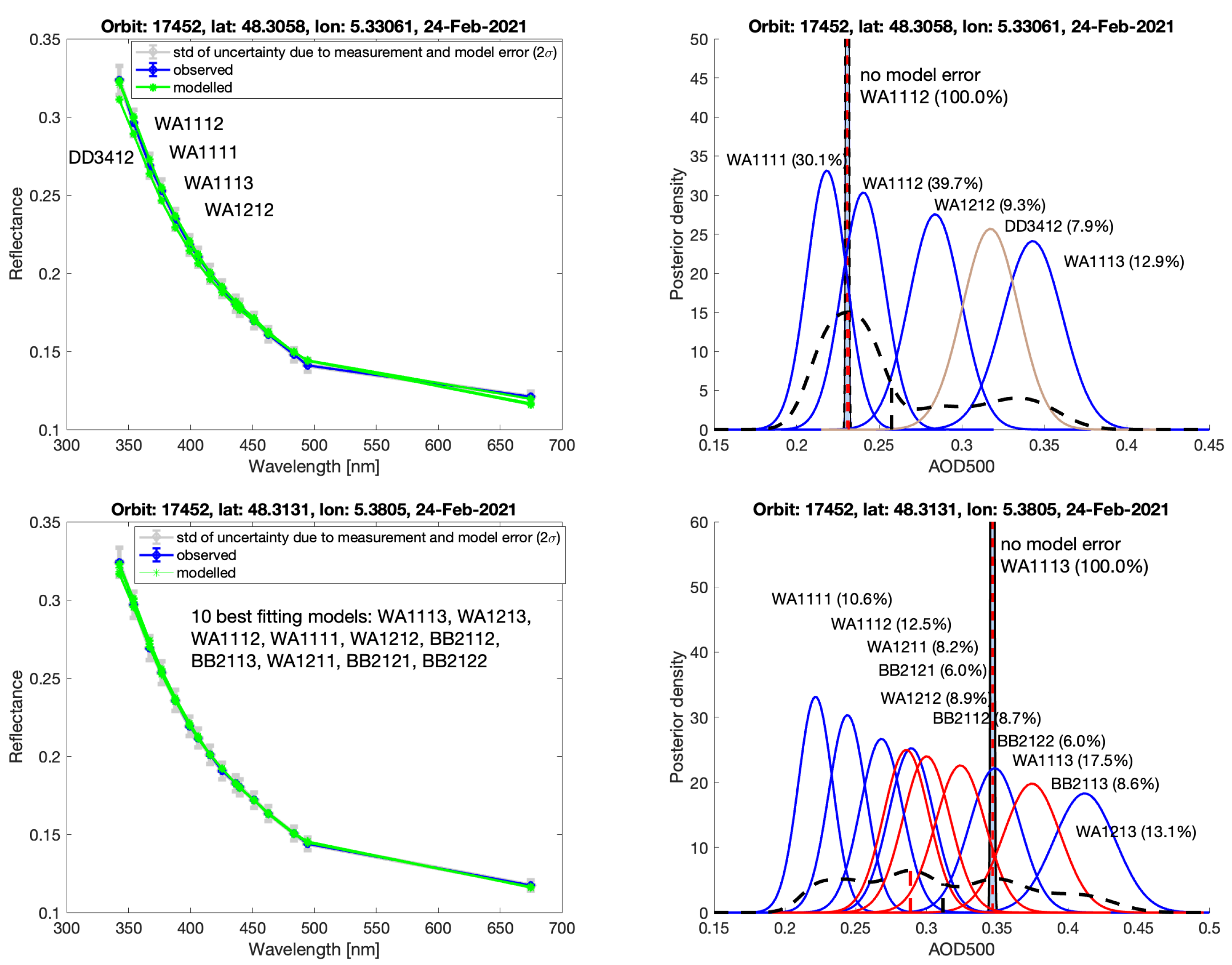
Figure 17 shows the results of two adjacent pixels (269,3200) (upper panels) and (270,3200) (bottom panels) located to the south-west of the AERONET site Bure_OPE (Figure 13). The results indicate that the predominant aerosol type is weakly absorbing and there are several models that can explain the observations. We can see that for both pixels the modelled reflectances match the observed reflectance (left panels). The averaged posterior distribution (Equation (10)), plotted as a dashed black line, has spread over the posteriors of AOD. Also, the uncertainty averaged over the selected models is very wide when the model discrepancy is involved (right panels). As a result the MAP AOD estimate in pixel (269,3200) is ∼0.23 and in pixel (270,3200) ∼0.29. When the model discrepancy was not accounted for, we obtained only one model and a more optimistic uncertainty. For the pixel (270,3200) we obtained a slightly different AOD estimate depending on whether the model error was included or not. A total of ten WA and BB type models are almost equally likely in the average posterior distribution of AOD, whereas for pixel (269,3200) (upper panels) the two models ‘WA1112’ and ‘WA1111’ dominate as indicated by the averaged posterior and relative evidence value (%) next to the model ID number. One of the most likely models is a dust model ‘DD3412’ that has a non-spherical particle shape (see Appendix A).
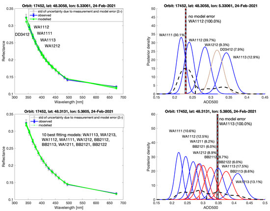
Figure 17.
On 24 February 2021, orbit: 17,452. Same as Figure 7 but for the two pixels (269,3200) (upper panels) and (270,3200) (bottom panels). The posterior density of AOD for each best-fitting model is shown on right-hand column in blue, red or brown depending on main aerosol type. The averaged posterior, based on the best-fitting models, is shown by a black dashed curve. The red vertical dashed line stands for the MAP AOD estimate from the averaged posterior, whereas the black vertical dashed line indicates the weighted mean of the MAP AOD estimates from the individual posteriors.
4. Discussion
The motivation for this study is to consider uncertainty arising from approximations in forward modelling and from the selection of the aerosol optical models. The focus is to provide a more realistic uncertainty estimate when retrieving AOD using satellite measurements and when the retrieval algorithm is based on pre-calculated aerosol optical models. Additionally, the proposed method allows for the study of the optical model selection process and its effect on the retrieved AOD and associated aerosol types. We have characterised the model discrepancy (i.e., the forward-model uncertainty) by applying a Gaussian process. The variance function of the Gaussian process quantifies the wavelength-dependent correlation structure of the discrepancy. The estimated model discrepancy is specific to this study because it depends on the retrieval setup (i.e., the aerosol optical models, the instrument noise level, the selected wavelength bands and the surface reflectance assumptions).
The advantage of the LUT-based algorithm is that it saves computation time, as the LUTs replace the most time-consuming part of the forward model run during the actual retrieval process. However, choosing only one model is not always meaningful, as several optical models can contribute to explaining the measurement. In our approach, the resulting AOD may be based on several optical models, but we also recognise the difficulty in model selection. We take into account uncertainty due to aerosol model selection using Bayesian model averaging tools. Overall, by utilising Bayesian techniques, we are able to analyse and determine uncertainty in a fairly straightforward manner.
The accuracy of the aerosol retrieval also depends on the correctness of the aerosol microphysical and optical properties (i.e., correspondence to reality), which are given to the radiative transfer run as input to create the LUTs. For instance, the particle shape can have a large effect on the scattering properties. Therefore, we have also included dust-type aerosol models whose particles are not spherical in order to study the selection of such models in the retrieval process. Naturally, the aerosol optical and microphysical properties involved do not cover all possible aerosol scenarios that can be provided as input data in the forward-model calculation. However, the method allows studying the ability to select the proper aerosol models from the LUTs and thus it can obtain valuable information about the process of model selection. For instance, if the averaged posterior density has more than one peak, i.e., the posterior is no longer Gaussian, it indicates difficulties in model selection.
We tested the performance of the retrieval algorithm through case studies using the actual satellite observations. The test cases include the detection of smoke aerosol particles transported across the Pacific Ocean, the detection of various types of desert dust in Africa and the detection of drifted dust in Europe. The results indicate that the proposed aerosol retrieval method can identify the expected types of aerosol, although the AOD levels obtained are not always comparable to those from AERONET AOD (500 nm). For example, in the case of the transported smoke (Section 3.1), the reason for the significant overestimation of AOD may be that we lack a biomass burning type of model with a wavelength-dependent imaginary part of the refractive index (e.g., [31]). Interestingly, dust models with a non-spherical particle shape were also selected as the best matching models for the solution (Section 3.2). This fits into the consensus on the use of spheroidal models in interpreting the remote sensing observations of dust aerosols (e.g., [33,34]). Still, in order to draw a conclusion about the retrieval accuracy, more exercises are needed with a comprehensive selection of different aerosol scenarios, including moderate aerosol cases. In addition, statistical comparison studies using, for example, monthly data from AERONET or other satellite aerosol products, could provide additional information on the functionality of the presented method. So far, we have only processed over-land pixels, but it is worth considering that over-ocean surfaces are included in further work.
The difficulty in satellite aerosol retrieval lies in accurately accounting for surface reflectivity and the coupling of the surface and atmosphere. The effect of an improper surface reflectance assumption on forward-model uncertainty has not been separately considered in this paper. However, surface reflectance is implicitly included in forward-model uncertainty, as the model discrepancy is empirically estimated based on the residuals of model fits.
The methodology presented for determining uncertainty estimates in combination with aerosol type and AOD retrieval could be useful, for example, in the following studies:
- Testing the retrieval method with aerosol optical models with different aerosol microphysical, optical and shape characteristics;
- Experimenting with how the method can detect and classify different aerosol situations and atmospheric ageing (such as aerosols near the source or transported aerosols);
- Studying the effect of different surface reflection assumptions on model selection and the resulting AOD.
Author Contributions
Conceptualisation, A.K. (Anu Kauppi), M.L. and J.T.; methodology, A.K. (Anu Kauppi), A.K. (Antti Kukkurainen), M.L. and J.T.; software, A.K. (Anu Kauppi) and A.K. (Antti Kukkurainen); formal analysis, A.K. (Anu Kauppi); investigation, A.K. (Anu Kauppi), A.K. (Antti Kukkurainen) and A.L.; data curation, A.K. (Anu Kauppi) and A.K. (Antti Kukkurainen); writing—original draft preparation, A.K. (Anu Kauppi); writing—review and editing, A.K. (Anu Kauppi), A.K. (Antti Kukkurainen), A.L., M.L., A.A., H.L. and J.T.; visualisation, A.K. (Anu Kauppi) and H.L.; project administration, J.T., M.L. and H.L.; funding acquisition, J.T., M.L. and H.L. All authors have read and agreed to the published version of the manuscript.
Funding
This research was funded by the Finnish Centre of Excellence in Inverse Modelling and Imaging granted by the Research Council of Finland grant number 353082. In addition, this work was supported by the Research Council of Finland projects ADAFUME grant number 321890 and CitySpot grant number 331829, and the Research Council of Finland’s Finnish Flagship Programme FAME grant number 359196.
Data Availability Statement
The TROPOMI/S5P level 1b and level 2 UV aerosol index products are available via the Copernicus Data Space Ecosystem (CDSE) (https://sentinels.copernicus.eu/web/sentinel/technical-guides/sentinel-5p/products-algorithms (accessed on 20 May 2024)). The created look-up tables and the results of the case studies are available on request from the corresponding author.
Acknowledgments
We would like to acknowledge by thanks the whole TROPOMI/S5P team. We thank the AERONET PIs and Co-Is and their staff for establishing and maintaining the Pilar_Cordoba, Medenine_IRA and Bure_OPE sites used in this investigation. The ADAM products were collected from the ADAM database (https://earth.esa.int/eogateway/catalog/adam-surface-reflectance-database-v4-0 (accessed on 20 May 2024)), and were produced by the ADAM team under the European Space Agency (ESA) study contract Nr C4000102979. We acknowledge the use of imagery from the NASA Worldview application (https://worldview.earthdata.nasa.gov (accessed on 20 May 2024)), part of the NASA Earth Observing System Data and Information System (EOSDIS). Special thanks to our colleagues at FMI; Päivi Haapanala for encouraging discussion about radiative attenuation by aerosols, Pekka Kolmonen for kind help with wavelength band issues and Petri Räisänen for friendly help providing the dust aerosol microphysical properties applied with ECHAM5 model.
Conflicts of Interest
The authors declare no conflicts of interest.
Appendix A. Description of Aerosol Properties and LUTs
The numbering of LUTs by identification (ID) number is executed on the same principle as is in the operational multi-wavelength OMI aerosol product (OMAERO; [35,36]), which is an LUT-based algorithm. The numbering of optical models helps to interpret the results (see Table A1) as the ID number distinguishes the subtypes of the main types of aerosol. The model ID number has four digits and is coded as: [main type][imaginary part of complex refractive index][vertical distribution][size distribution]. The main type number is ‘1’ for WA models, ‘2’ for BB models and ‘3’ for DD models. Additionally, the vertical distribution has three categories for the BB and DD models according to the aerosol vertical layer. The vertical atmosphere layers are the following: 0–2 km (‘1’), 2–4 km (‘2’) and 4–6 km (‘3’). The complex refractive index is divided into the real and imaginary parts. The real part affects the scattering properties of the particles in the radiative transfer model. It has here a constant value varying according to the aerosol type. The imaginary part of the refractive index indicates the strength of the absorption, and varies according to the aerosol type. In our study, only the dust models have a wavelength-dependent imaginary part. The size distribution is given as a bimodal log-normal function or as the mean particle radius with the standard deviation. For more details, see the references listed in Table A1.
Table A1.
The LUTs categorised by the main types WA, BB and DD. The third digit (’x’) in the model ID number has a range of 1–3 indicating different vertical distributions.
Table A1.
The LUTs categorised by the main types WA, BB and DD. The third digit (’x’) in the model ID number has a range of 1–3 indicating different vertical distributions.
| Type | Model ID | References |
|---|---|---|
| WA | 1111, 1112, 1113 | [17,35,36] |
| WA | 1211, 1212, 1213 | [17,35,36] |
| WA | 1311, 1312, 1313 | [17,35,36] |
| BB | 21 × 1, 21 × 2, 21 × 3 | [17,35,36] |
| BB | 22 × 1, 22 × 2, 22 × 3 | [17,35,36] |
| BB | 23 × 1, 23 × 2, 23 × 3 | [17,35,36] |
| DD | 31 × 1, 31 × 2 | [17,35,36] |
| DD | 32 × 2, 32 × 2 | [17,35,36] |
| DD | 33 × 1, 33 × 2 | [37] (particle shape: spherical) |
| DD | 34 × 1, 34 × 2 | [37] (particle shape: prolate spheroid) |
| DD | 35 × 1, 35 × 2 | [38,39] |
In principle, we have utilised the aerosol microphysical properties from the OMI OMAERO LUTs when assigning aerosol size distribution and refractive index for the aerosol models (see the references in Table A1). Additionally, we have included other dust type models whose physical properties (i.e., size distribution and refractive index) have been collected from the literature (Table A1). In particular, we have included six dust models ’34xx’ that have a spheroidal particle shape instead of a spherical one. These aerosol physical properties are from the Cairo 2 sample collected from the Northern Sahara (see Tables 1 and 5 in [37]) and we used prolate spheroids with an aspect ratio of 0.25. In reality, the dust particles are also not perfect spheroids but have a variety of different shapes (e.g., [37,40]).
For example, the two dust models, ’DD3311’ and ’DD3411’, differ solely in the shape of the dust model particle. These two dust models were obtained as a solution in the second case study (see Section 3.2 and Figure 16c,d). The implications of the particle shape to the key optical properties are depicted in Figure A1. The angular distribution of scattered intensity S11 shows (Figure A1a) that the shape has a larger impact on S11 for smaller wavelengths, i.e., when the particles are relatively larger as compared to the wavelength. The spheroidal particles are more forward-scattering, while the spherical particles can have up to five times stronger back-scattered intensity. This difference decreases significantly for larger wavelengths. The SSA shows (Figure A1b) that the non-spherical particles scatter light relatively more than the spherical particles for wavelengths smaller than 650 nm. For larger wavelengths, the spherical particles scatter more light than the non-spherical particles, which is also seen to have an impact on AOD (Figure A1d). The Ångström exponent shows (Figure A1c) a large difference between the two shapes despite the equal volumes of the individual particles. The Ångström exponent in the LUT is set to zero at the reference wavelength 500 nm. Due to the shape difference, the physical sizes of the particles differ, which is reflected in the resulting Ångström exponent values.
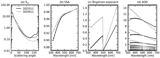
Figure A1.
Differences in the optical properties of spherical (black lines, ‘DD3311’) and non-spherical particles (grey lines, ‘DD3411’). (a) The angular distribution of the intensity of scattered light (S11) is shown with solid lines for UV and dashed lines for the largest wavelength considered. (b) SSA shows the relative strength of scattering to total extinction as a function of wavelength. (c) The wavelength dependence of the Ångström exponent for both particle shapes. (d) AOD from the radiative transfer computations using these two particle models.

References
- Povey, A.C.; Grainger, R.G. Known and unknown unknowns: Uncertainty estimation in satellite remote sensing. Atmos. Meas. Tech. 2015, 8, 4699–4718. [Google Scholar] [CrossRef]
- Sayer, A.M.; Govaerts, Y.; Kolmonen, P.; Lipponen, A.; Luffarelli, M.; Mielonen, T.; Patadia, F.; Popp, T.; Povey, A.C.; Stebel, K.; et al. A review and framework for the evaluation of pixel-level uncertainty estimates in satellite aerosol remote sensing. Atmos. Meas. Tech. 2020, 13, 373–404. [Google Scholar] [CrossRef]
- Lipponen, A.; Kolehmainen, V.; Kolmonen, P.; Kukkurainen, A.; Mielonen, T.; Sabater, N.; Sogacheva, L.; Virtanen, T.H.; Arola, A. Model-enforced post-process correction of satellite aerosol retrievals. Atmos. Meas. Tech. 2021, 14, 2981–2992. [Google Scholar] [CrossRef]
- Veefkind, J.P.; Aben, I.; McMullan, K.; Förster, H.; de Vries, J.; Otter, G.; Claas, J.; Eskes, H.J.; de Haan, J.F.; Kleipool, Q.; et al. TROPOMI on the ESA Sentinel-5 Precursor: A GMES mission for global observations of the atmospheric composition for climate, air quality and ozone layer applications. Remote Sens. Environ. 2012, 120, 70–83. [Google Scholar] [CrossRef]
- Stein Zweers, D.C. TROPOMI ATBD of the UV Aerosol Index; S5P-KNMI-L2-0008-RP; Royal Netherlands Meteorological Institute: De Bilt, The Netherlands, 2018; Issue 1.1; p. 30. [Google Scholar]
- Kooreman, M.L.; Stammes, P.; Trees, V.; Sneep, M.; Tilstra, L.G.; de Graaf, M.; Stein Zweers, D.C.; Wang, P.; Tuinder, O.N.E.; Veefkind, J.P. Effects of clouds on the UV Absorbing Aerosol Index from TROPOMI. Atmos. Meas. Tech. 2020, 13, 6407–6426. [Google Scholar] [CrossRef]
- Sun, J.; Veefkind, P.; Nanda, S.; van Velthoven, P.; Levelt, P. The role of aerosol layer height in quantifying aerosol absorption from ultraviolet satellite observations. Atmos. Meas. Tech. 2019, 12, 6319–6340. [Google Scholar] [CrossRef]
- Torres, O.; Jethva, H.; Ahn, C.; Jaross, G.; Loyola, D.G. TROPOMI aerosol products: Evaluation and observations of synoptic-scale carbonaceous aerosol plumes during 2018–2020. Atmos. Meas. Tech. 2020, 13, 6789–6806. [Google Scholar] [CrossRef]
- Rao, L.; Xu, J.; Efremenko, D.S.; Loyola, D.G.; Doicu, A. Optimization of Aerosol Model Selection for TROPOMI/S5P. Remote Sens. 2021, 13, 2489. [Google Scholar] [CrossRef]
- Määttä, A.; Laine, M.; Tamminen, J.; Veefkind, J.P. Quantification of uncertainty in aerosol optical thickness retrieval arising from aerosol microphysical model and other sources, applied to Ozone Monitoring Instrument (OMI) measurements. Atmos. Meas. Tech. 2014, 7, 1185–1199. [Google Scholar] [CrossRef]
- Mayer, B.; Kylling, A. Technical note: The libRadtran software package for radiative transfer calculations—Description and examples of use. Atmos. Chem. Phys. 2005, 5, 1855–1877. [Google Scholar] [CrossRef]
- Emde, C.; Buras-Schnell, R.; Kylling, A.; Mayer, B.; Gasteiger, J.; Hamann, U.; Kylling, J.; Richter, B.; Pause, C.; Dowling, T.; et al. The libRadtran software package for radiative transfer calculations (version 2.0.1). Geosci. Model Dev. 2016, 9, 1647–1672. [Google Scholar] [CrossRef]
- MacKay, D.J.C. Bayesian interpolation. Neural Comput. 1992, 4, 415–447. [Google Scholar] [CrossRef]
- Spiegelhalter, D.J.; Best, N.G.; Carlin, B.P.; van der Linde, A. Bayesian measures of model complexity and fit. J. R. Stat. Soc. Ser. B Stat. Methodol. 2002, 64, 583–639. [Google Scholar] [CrossRef]
- Kennedy, M.C.; O’Hagan, A. Bayesian Calibration of Computer Models. J. R. Stat. Soc. B 2001, 63, 425–464. [Google Scholar] [CrossRef]
- Brynjarsdóttir, J.; O’Hagan, A. Learning about physical parameters: The importance of model discrepancy. Inverse Probl. 2014, 30. [Google Scholar] [CrossRef]
- Veihelmann, B.; Levelt, P.F.; Stammes, P.; Veefkind, J.P. Simulation study of the aerosol information content in OMI spectral reflectance measurements. Atmos. Chem. Phys. 2007, 7, 3115–3127. [Google Scholar] [CrossRef]
- Leloux, J.; Rozemeijer, N.; van Swol, R.; Vonk, F. Input/Output Data Specification for the TROPOMI L01b Data Processor; S5P-KNMI-L01B-0012-SD, CI-6510-IODS; Royal Netherlands Meteorological Institute: De Bilt, The Netherlands, 2022; Issue 11.0.0; p. 116. [Google Scholar]
- Apituley, A.; Pedergnana, M.; Sneep, M.; Veefkind, J.P.; Loyola, D.; Stein Zweers, D. Sentinel-5 Precursor/TROPOMI Level 2 Product User Manual UV Aerosol Index; S5P-KNMI-L2-0026-MA, CI-7570-PUM; Royal Netherlands Meteorological Institute: De Bilt, The Netherlands, 2018; Issue 1.0.0; p. 116. [Google Scholar]
- Holben, B.N.; Eck, T.F.; Slutsker, I.; Tanré, D.; Buis, J.P.; Setzer, A.; Vermote, E.; Reagan, J.A.; Kaufman, Y.J.; Nakajima, T.; et al. AERONET—A federated instrument network and data archive for aerosol characterization. Remote Sens. Environ. 1998, 66, 1–16. [Google Scholar] [CrossRef]
- Giles, D.M.; Sinyuk, A.; Sorokin, M.G.; Schafer, J.S.; Smirnov, A.; Slutsker, I.; Eck, T.F.; Holben, B.N.; Lewis, J.R.; Campbell, J.R.; et al. Advancements in the Aerosol Robotic Network (AERONET) Version 3 database – automated near-real-time quality control algorithm with improved cloud screening for Sun photometer aerosol optical depth (AOD) measurements. Atmos. Meas. Tech. 2019, 12, 169–209. [Google Scholar] [CrossRef]
- Shin, S.K.; Tesche, M.; Noh, Y.; Müller, D. Aerosol-type classification based on AERONET version 3 inversion products. Atmos. Meas. Tech. 2019, 12, 3789–3803. [Google Scholar] [CrossRef]
- Dubovik, O.; King, M.D. A flexible inversion algorithm for retrieval of aerosol optical properties from sun and sky radiance measurements. J. Geophys. Res. 2000, 105, 20673–20696. [Google Scholar] [CrossRef]
- Gasteiger, J.; Wiegner, M. MOPSMAP v1.0: A versatile tool for the modeling of aerosol optical properties. Geosci. Model Dev. 2018, 11, 2739–2762. [Google Scholar] [CrossRef]
- Gelman, A.; Carlin, J.B.; Stern, H.S.; Dunson, D.B.; Vehtari, A.; Rubin, D.B. Bayesian Data Analysis, 3rd ed.; Chapman & Hall/CRC: Boca Raton, FL, USA, 2013. [Google Scholar]
- Chandrasekhar, S. Radiative Transfer; Dover Publ.: New York, NY, USA, 1960. [Google Scholar]
- Rasmussen, C.E.; Williams, C.K.I. Gaussian Processes for Machine Learning; The MIT Press: Cambridge, MA, USA, 2006. [Google Scholar]
- Banerjee, S.; Carlin, B.P.; Gelfand, A.E. Hierarchical Modeling and Analysis for Spatial Data; Chapman and Hall/CRC Press: Boca Raton, FL, USA, 2004. [Google Scholar]
- O’Neill, N.T.; Ignatov, A.; Holben, B.N.; Eck, T.F. The lognormal distribution as a reference for reporting aerosol optical depth statistics; Empirical tests using multi-year, multi-site AERONET sunphotometer data. Geophys. Res. Lett. 2000, 27, 3333–3336. [Google Scholar] [CrossRef]
- Hoeting, J.A.; Madigan, D.; Raftery, A.E.; Volinsky, C.T. Bayesian Model averaging: A Tutorial. Statist. Sci. 1999, 14, 382–417. [Google Scholar]
- Jethva, H.; Torres, O. Satellite-based evidence of wavelength-dependent aerosol absorption in biomass burning smoke inferred from Ozone Monitoring Instrument. Atmos. Chem. Phys. 2011, 11, 10541–10551. [Google Scholar] [CrossRef]
- González, R.; Toledano, C.; Román, R.; Mateos, D.; Asmi, E.; Rodríguez, E.; Lau, I.C.; Ferrara, J.; D’elia, R.; Antuña-Sánchez, J.C.; et al. Characterization of Stratospheric Smoke Particles over the Antarctica by Remote Sensing Instruments. Remote Sens. 2020, 12, 3769. [Google Scholar] [CrossRef]
- Dubovik, O.; Sinyuk, A.; Lapyonok, T.; Holben, B.N.; Mishchenko, M.; Yang, P.; Eck, T.F.; Volten, H.; Munõz, O.; Veihelmann, B.; et al. Application of spheroid models to account for aerosol particle nonsphericity in remote sensing of desert dust. J. Geophys. Res. 2006, 111, D11208. [Google Scholar] [CrossRef]
- Merikallio, S.; Lindqvist, H.; Nousiainen, T.; Kahnert, M. Modelling light scattering by mineral dust using spheroids: Assessment of applicability. Atmos. Chem. Phys. 2011, 11, 5347–5363. [Google Scholar] [CrossRef]
- Torres, O.; Tanskanen, A.; Veihelmann, B.; Ahn, A.; Braak, R.; Bhartia, P.K.; Veefkind, P.; Levelt, P. Aerosols and Surface UV Products from Ozone Monitoring Instrument Observations: An Overview. J. Geophys. Res. 2007, 112, D24S47. [Google Scholar] [CrossRef]
- Curier, R.L.; Veefkind, J.P.; Braak, R.; Veihelmann, B.; Torres, O.; de Leeuw, G. Retrieval of aerosol optical properties from OMI radiances using a multiwavelength algorithm: Application to western Europe. J. Geophys. Res. 2008, 113, D17S90. [Google Scholar] [CrossRef]
- Wagner, R.; Ajtai, T.; Kandler, K.; Lieke, K.; Linke, C.; Müller, T.; Schnaiter, M.; Vragel, M. Complex refractive indices of Saharan dust samples at visible and near UV wavelengths: A laboratory study. Atmos. Chem. Phys. 2012, 12, 2491–2512. [Google Scholar] [CrossRef]
- Zhang, K.; O’Donnell, D.; Kazil, J.; Stier, P.; Kinne, S.; Lohmann, U.; Ferrachat, S.; Croft, B.; Quaas, J.; Wan, H.; et al. The global aerosol-climate model ECHAM-HAM, version 2: Sensitivity to improvements in process representations. Atmos. Chem. Phys. 2012, 12, 8911–8949. [Google Scholar] [CrossRef]
- Räisänen, P.; Haapanala, P.; Chung, C.E.; Kahnert, M.; Makkonen, R.; Tonttila, J.; Nousiainen, T. Impact of dust particle non-sphericity on climate simulations. Q. J. R. Meteorol. Soc. 2013, 139, 2222–2232. [Google Scholar] [CrossRef]
- Lindqvist, H.; Jokinen, O.; Kandler, K.; Scheuvens, D.; Nousiainen, T. Single scattering by realistic, inhomogeneous mineral dust particles with stereogrammetric shapes. Atmos. Chem. Phys. 2014, 14, 143–157. [Google Scholar] [CrossRef]


Disclaimer/Publisher’s Note: The statements, opinions and data contained in all publications are solely those of the individual author(s) and contributor(s) and not of MDPI and/or the editor(s). MDPI and/or the editor(s) disclaim responsibility for any injury to people or property resulting from any ideas, methods, instructions or products referred to in the content. |
© 2024 by the authors. Licensee MDPI, Basel, Switzerland. This article is an open access article distributed under the terms and conditions of the Creative Commons Attribution (CC BY) license (https://creativecommons.org/licenses/by/4.0/).