Abstract
Oceanic trajectories frequently exhibit multiple periodic patterns across various time intervals, e.g., tidal variations, mesoscale eddies, and El Niño events correspond to diurnal, seasonal, and interannual fluctuations in environmental factors. To explore hidden spatiotemporal multiple periodic behaviors in noisy ocean data, we propose a novel trajectory clustering method, namely DTID-STFC. It first identifies dense time intervals (DTIs) in which trajectories occur frequently. Subsequently, within each DTI, it utilizes spectral embedding to project trajectories onto a latent subspace and proposes three-way fuzzy clustering to obtain results. We evaluate the proposed method on simulated datasets and compare it with traditional and state-of-the-art trajectory clustering approaches. Experimental results indicate that it outperforms other methods across all five metrics. Moreover, when applying the DTID-STFC method to the analysis of mesoscale cyclonic eddies in the South China Sea and vessel data, it demonstrates more discernible results than traditional methods, and it aligns well with physical oceanographic processes. This proposed method offers valuable insights into identifying periodic behaviors from complex and noisy spatiotemporal oceanic trajectory data.
1. Introduction
Trajectories in the ocean can primarily be categorized into two types: those shaped by meteorological forces, such as tropical cyclones, and those influenced by human intervention, such as vessel routes. This paper delves into an exploration of these two distinct types of oceanic trajectory data, aiming to uncover their underlying dynamics and significance. Exploring the periodic patterns within these trajectories is crucial for comprehending ocean processes, such as heat transfer and resource transportation. Trajectory clustering is one of the most powerful data mining tools that group similar spatial trajectories and identify implicit movement patterns [1,2,3]. However, the periodic patterns analysis based on oceanic trajectory clustering can be challenging due to their manifestation of significant diurnal, seasonal, and interannual variations, which are influenced by intricate environmental factors. For example, the paths of tropical cyclones adhere to regular patterns with monsoon seasonal cycles [4], and ocean bacterioplankton displays oscillating diurnal rhythms [5]. Moreover, these trajectories may exhibit multiple periodic behaviors over time. For example, the monsoon currents [6] between the Arabian Sea and the Bay of Bengal flow eastward and westward during the periods of May to September and November to February, respectively. To more insightfully capture the periodicity within oceanic trajectories, a methodology is needed to cluster trajectories based on trajectory temporal distribution rather than solely on spatial proximity.
Existing trajectory clustering methods are categorized into three groups. (1) Point-based clustering: Clustering is performed based on individual points in trajectories. These methods are often employed to analyze spatiotemporal distribution [7] and discover points of interest [8,9]. Li et al. [10] proposed a two-phase approach to detect urban hotspots using taxi data. Specifically, in the first phase, the spatiotemporal hierarchical density-based spatial clustering of applications with noise (HDBSCAN) was used to cluster trajectory points. In the second phase, they introduced the concept of region growing to further filter noise and utilized the route distance to measure the spatial similarity. Liu et al. [2] employed k-means to examine the movement patterns of tourists on Mount Huashan in China, utilizing open GPS-trajectory data points. (2) Sub-trajectory clustering: It involves the segmentation of trajectories into sub-trajectories and clustering them, which can be employed to investigate the local information of trajectories [11,12,13]. TRACLUS [11] is one of the most classic sub-trajectory clustering algorithms. It segments trajectories into segments based on the minimum description length principle and subsequently constructs groups of similar segments using the extended density clustering algorithm. For spatiotemporal segments, Ansari et al. [14] developed a sub-trajectory clustering algorithm by extending the density-based spatial clustering of applications with noise (DBSCAN) and introducing a temporal threshold to mine spatiotemporal co-location events. Considering that trajectory data can be rich in dimensions beyond just the spatial and temporal dimensions, Bermingham and Lee [15] proposed a general sub-trajectory clustering methodology designed to identify clusters for the better utilization of diverse spatial data. The proposed methodology first segments the trajectories and then employs an R-tree-based search to identify segments with similar distances. Subsequently, DBSCAN is applied to group these segments into clusters. (3) Whole trajectory clustering: This involves grouping similar complete trajectories to discover general movement patterns and recurring behaviors. MTCA [16] obtains different whole trajectory clusters to discover regular behaviors by calculating the multidimensional Hausdorff distance and utilizing the DBSCAN algorithm. For vehicle trajectories in transportation networks, Hong et al. [17] proposed a spatiotemporal trajectory clustering method, which includes adopting the time-dependent shortest-path distance measurement and taking advantage of the topological relations of a predefined network to discover the shared sub-paths and identify trip patterns.
Most trajectory clustering methods typically concentrate on grouping spatiotemporally similar trajectories without delving into their underlying variations over time. This restricts their ability to conduct a more nuanced analysis of how oceanic periodic patterns evolve across different seasons or time intervals. For example, marine organisms may have different migration behaviors under different seasonal climate conditions. Furthermore, noise is universal in oceanic trajectories data, which challenges the stability and accuracy of results. Some studies employed density-based methods robust to noise, such as DBSCAN [18,19,20,21], HDBSCAN [22], and density peak clustering (DPC) [13]. However, their effectiveness is limited when dealing with complex datasets characterized by non-uniform density.
Spectral clustering [23] has shown good performance in handling various data structures, which regards trajectories as nodes in a graph with edges represented by similarity. The data are projected into a lower-dimensional subspace through spectral embedding, capturing essential information while mitigating the dimensionality curse for oceanic trajectories. Nonetheless, spectral clustering struggles to identify noise trajectories, and it is prone to incorrectly assign them to clusters and compromise accuracy. In contrast, fuzzy c-means (FCM) [24] is robust to noise and computes the probabilities of trajectories belonging to all clusters. Yet, for trajectories with clearly specific classes, the results lack intuitiveness and require manual empirical judgement. In recent years, deep learning methods including long short-term memory (LSTM) [25] and bi-directional LSTM networks [26] have gained significant attention in trajectory clustering. These methods encode trajectories and transform them into feature vectors. But deep learning models often function as black boxes, making the inference process unexplainable and obscured from view.
To overcome the challenges posed by noisy trajectories and intricate data structures, we develop a new trajectory clustering method to mine multiple periodic patterns for complex oceanic trajectories. Unlike the conventional methods, we first develop a trajectory-dense time interval detection (DTID) algorithm to efficiently identify dense time intervals where trajectories frequently happen by leveraging their temporal distribution. We then propose spectral three-way fuzzy clustering (STFC) to cluster trajectories within the same dense time intervals identified by DTID. STFC leverages the strengths of spectral embedding [23] for handling various data structures and incorporates three-way fuzzy clustering to handle noise effectively. Finally, we identify spatiotemporal periodic behaviors from noisy and complex oceanic data by obtaining clusters of trajectories with similar motion patterns within the same time interval.
The remainder of this paper is organized as follows: Section 2 presents key definitions and symbols. Section 3 presents the proposed method and implementation details. The experimental results and discussion are displayed in Section 4 and Section 5, respectively. Finally, Section 6 concludes the paper and discusses promising directions for future research.
2. Definitions and Symbols
In this section, we provide definitions and symbols of key terms.
Definition 1.
Trajectory (): A sequence that describes the path of an object over time and space. It consists of data points sampled at uniform time intervals that are arranged chronologically. represents the th trajectory.
Definition 2.
Dense Time Interval (): A time interval in which object activity or behavior occurs more frequently, composed of a starting time and an ending time. represents the th dense time interval.
Definition 3.
Trajectory Cluster (): A grouping of trajectories within the dataset that display similar behavioral patterns or characteristic variations. represents the th cluster.
The symbols with their definition are presented in Table 1.

Table 1.
Symbol definition.
3. The Proposed Method
The proposed oceanic trajectories clustering method, namely DTID-STFC, is able to perform spatiotemporal clustering considering periodical variations of trajectories. Our method consists of two main parts, as shown in Figure 1: (1) TR-dense time interval detection (DTID) identifies frequently occurring time intervals within the trajectories and captures the intrinsic temporal dependencies by leveraging the temporal distributions of trajectory. (2) Spectral three-way fuzzy clustering (STFC) groups trajectories exhibiting similar behaviors within each dense time interval.
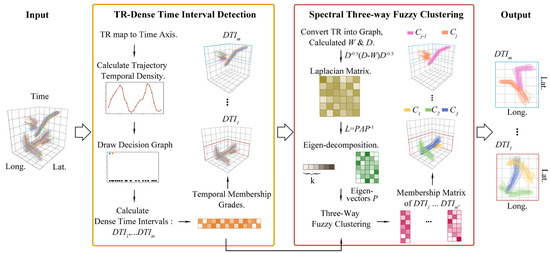
Figure 1.
The proposed method framework consists of two main parts: dense time interval detection and spectral three-way fuzzy clustering.
3.1. TR-Dense Time Interval Detection
Due to the influence of specific temporal and environmental factors in ocean regions, oceanic trajectories often display unique periodic patterns, which vary according to different time frames (e.g., seasons). Within roughly comparable time frames, these trajectories frequently manifest similar behavioral tendencies. The identification of distinct dense time intervals within trajectories offers a valuable opportunity to gain deeper insight into why some events tend to frequently occur during specific periods.
Based on the fast search and discovery of density peaks clustering [27] algorithm, we develop an efficient dense time interval detection (DTID) algorithm by analyzing the time distributions of trajectories. The flowchart of DTID is shown in Figure 2.
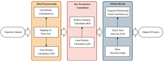
Figure 2.
The flowchart of DTID.
Initially, we map trajectories onto the time axis and calculate the unit density at each time point , representing the number of trajectories present at that time point. Taking the Automatic Identification System (AIS) vessel data [28] from 2012 to 2016 as an example, we project the trajectories onto a 24 h temporal axis with hourly units. Two peaks can be observed in Figure 3a, indicating that vessels mainly focus on activities during these two intervals. To identify dense time intervals within trajectories, it is necessary to pinpoint division points on the time axis. We assume that (1) the local density of division points is lower than their neighbors, and (2) the distances between division points are relatively large.
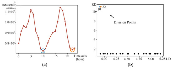
Figure 3.
Example of applying DTID to AIS vessel data. (a) Trajectory temporal density; (b) decision graph. The points circled with different color circles in (a) correspond to the division points of different colors in (b).
To satisfy the two mentioned assumptions, the local density (LD) and relative distance (RD) are computed for each time point on the time axis. LD is calculated as the sum of unit density within the time window (TW), as shown in Equation (1), where represents the length of the time axis. RD is calculated based on the distance between time point and the time point with smaller local density as Equation (2).
Based on the LD and RD, a decision graph is generated to determine the number and values of division points. The decision graph of AIS vessel trajectories is shown in Figure 3b, where the TW size is set to 4.8 (24 × 0.2). From Figure 3a, we can observe two division points: 10 and 22, which divide the 24 h period into two distinct dense time intervals: 10:00–21:00 and 22:00–09:00. If the dataset is concentrated within a single time interval, or if there are no intervals of high occurrence, the decision graph will not contain division points.
For trajectories spanning multiple time intervals, we propose the concept of temporal membership grade for trajectories and quantitatively compute it using Equation (3), which calculates the trajectory’s length of time within a dense time interval divided by its total time period. In Equation (3), and denote the start time of and , respectively; and denote the end time of and , respectively.
3.2. Spectral Three-Way Fuzzy Clustering
To effectively group similar behaviors from the noisy and complex oceanic trajectory data, we propose a spectral three-way fuzzy clustering algorithm. This algorithm involves spectral embedding to handle the intricate dataset and three-way fuzzy clustering to reduce interference from noisy trajectories on the final results.
In spectral embedding [23], the affinity matrix is firstly computed according to Equation (4). Here, denotes the trajectory distance between and , which is measured using dynamic time warping (DTW) algorithm [29,30]. Degree matrix is a diagonal matrix with the th entry . The normalized Laplacian matrix is then derived from and as shown in Equation (5). Next, eigen-decomposition of the normalized Laplacian matrix is carried out to extract the eigenvectors corresponding to the smallest eigenvalues . This process projects the trajectories into a lower-dimensional spectral space, with eigenvectors representing the new coordinates .
The three-way fuzzy clustering takes eigenvectors as the input and outputs three-way membership grades, which reflect the probability of each belonging to different clusters. In contrast to traditional fuzzy clustering algorithms, which often assume that samples belong to all clusters, three-way fuzzy clustering grounded in Three-Ways Decision Theory [31] introduces the concept of “not belonging”, thereby allowing samples to exist in an intermediate or definite state of membership.
To obtain the three-way membership grades of each , inspired by FCM [24], we first calculate the membership grade of the in as shown in Equation (6).
where denotes the distance between the and .
Then, we calculate the three-way membership grade of the based on the computed . When a trajectory’s membership grade in a specific cluster or clusters significantly exceeds the membership grades in other clusters, the trajectory is considered to belong to the specific cluster or clusters. In such cases, the trajectory’s membership grades in other clusters are set to 0, thereby achieving the “not belonging” judgment. The calculation of the three-way membership grade is shown in Equation (7), where ε represents the three-way threshold, and denotes the set of membership grades with the minimum number, for which the sum is required to be greater than .
Finally, considering the varying temporal membership grades of different trajectories within each time interval, cluster centers are determined using the calculated three-way membership grade and the trajectories’ temporal membership grade with respect to , as shown in Equation (8).
The DTID-STFC algorithm is detailed in Algorithm 1.
| Algorithm 1: Dense time interval detection and spectral three-way fuzzy clustering (DTID-STFC) (Pseudocode for the DTID-STFC: /*** and ***/ represents explanatory content) | |
| Input: Trajectory dataset <, the time window size rate , the three-way threshold . | |
| /*** Dense time interval detection ***/ | |
| Initialization: (1) Construct the time axis based on trajectory data, including the length and units of the time axis. (2) Calculate the unit density of trajectories on the time axis. (3) Calculate the time window. | |
| 1: | For each time point on the time axis: |
| 2: | Calculate using Equation (1). |
| 3 | For each time point on the time axis: |
| 4: | Calculate using Equation (2). |
| 5: | Draw decision graph to determine the dense time intervals . |
| 6: | For each trajectory : |
| 7: | Calculate temporal membership grade using Equation (3). |
| /*** Spectral three-way fuzzy clustering ***/ | |
| 8: | For each dense : |
| 9: | /*** Determine the optimal value based on the quality of clustering results. ***/ |
| 10: | Construct the affinity matrix of trajectories occurring in using Equation (4). |
| 11: | Construct the degree matrix calculated by . |
| 12: | Initialize the three-way membership grade matrix using random floating-point numbers between 0 and 1. |
| 13: | ; // Equation (5). |
| 14: | Eigenvalues, eigenvectors = eigen decomposition (). |
| 15: | Sort(eigenvalues). |
| 16: | Select the eigenvectors corresponding to the smallest eigenvalue as the new coordinates in the spectral space, where the th row vector is defined as . |
| 17: | While not converged do |
| 18: | /*** Convergence experiment: ***/ |
| 19: | Calculate the centroids based on and using Equation (8). |
| 20: | Calculate cluster membership grade matrix using Equation (6). |
| 21: | Update three-way membership grade matrix based on using Equation (7). |
| 22: | /*** Convergence experiment: and ***/ |
| 23: | End while. |
| 24: | Output: the three-way membership grade matrix corresponding to . |
3.3. Computational Complexity Analysis
From the calculation process presented in Section 3.1 and Section 3.2, our method consists of two main parts. In the DTID, the main focus is on the calculation of LD, RD, and on the time axis. Thus, the computational complexity of DTID is where denotes the length of time axis. In the STFC, it is necessary to compute the dissimilarity between trajectories, perform eigen-decomposition with a time complexity of , and apply three-way fuzzy clustering. In this paper, we adopt the DTW algorithm to calculate trajectory dissimilarity, and the time complexity of DTW is , where represents the maximum length of trajectories. Taking the above analyses into account, the time complexity of STFC is , where denotes the convergent iteration of spectral three-way fuzzy clustering.
4. Experimental Results
To objectively evaluate the performance of the proposed DTID-STFC method, we generate a simulated trajectory dataset with ground truth. Subsequently, we apply DTID-STFC to a real-world oceanic dataset, mesoscale cyclonic eddies, and AIS vessel trajectories, to showcase its capability in discovering multiple periodic patterns.
4.1. Datasets
Dataset 1: We use the trajectory generation program [32] to generate a two-dimensional spatial trajectory dataset with five different classes, each having varying lengths and locations. We randomly select a portion of the trajectories in the first class and reverse their directions. For the second class, we select a portion of the trajectories and multiply their speeds by two. We add time, speed, and turning angle attributes to the dataset, resulting in a five-dimensional dataset with features including time (ranging from 0 to 100), x-coordinate, y-coordinate, velocity, and angle. Additionally, 10 noisy trajectories of varying lengths are added to the dataset. Finally, we manually assign labels of trajectories based on their features, which are used for comparison with the clustering results. The different feature details in the five classes can be seen in Table 2.
Table 2.
Detailed information of Dataset 1.
Dataset 2: We utilize the altimetric Mesoscale Eddy Trajectories [33], detected from multiple satellite mission altimetry datasets and released by the Archiving, Validation and Interpretation of Satellite Oceanographic data (AVISO) with the support of the Copernicus Marine Environment Monitoring Service (CMEMS). The spatial resolution of the data is 0.25° × 0.25°, with a temporal resolution of one day, saved in the NetCDF file format. We select mesoscale cyclonic eddy trajectories in the South China Sea region (109°E–121°E, 3°N–23°N) from 1 January 1993 to 9 February 2022, with lifetimes exceeding 10 consecutive days. The preprocessed data contain 3976 trajectories with 141,938 sampling points.
Dataset 3: The AIS fishing vessel dataset [28], released by Global Fishing Watch and available publicly at https://globalfishingwatch.org/data-download/datasets/public-training-data-v1 (accessed on 28 January 2024), is stored in CSV file format with a file size of 801 MB. We extracted fishing vessel data covering the period from 2012 to 2016, specifically targeting vessels with lifetimes exceeding 10 consecutive days. The dataset contains attributes such as MMSI (vessel identifier), time, speed, latitude, and longitude coordinates. Following preprocessing, the dataset consists of 3212 trajectories with a total of 55,393 sampling points.
4.2. Evaluation Metrics
In the experiments, we employ two external evaluation metrics, normalized mutual information (NMI) [34] and adjusted rand index (ARI) [35], as well as three internal evaluation metrics, Calinski–Harabasz index (CHI) [36], Silhouette Coefficient [37], and Davies–Bouldin index (DBI) [38], to assess the quality of the clustering results. Larger values of NMI, ARI, CHI, and the Silhouette Coefficient indicate better results, while smaller values of DBI represent higher clustering quality.
4.3. Experiment in Simulated Trajectory
First, DTID is applied to detect the dense time intervals in Dataset 1 with the time window (TW) size set to 20 (100 × 20). From Figure 4a, it can be observed that Dataset 1 exhibits three peaks in the distribution of trajectory timestamps. The decision graph in Figure 4b shows division points at 0, 25, and 50, allowing us to divide the time into three intervals, (0–24), (25–49), and (50–99), which is consistent with the predetermined time scope in Dataset 1. This verifies the effectiveness of DTID in detecting dense time interval distributions of trajectories.
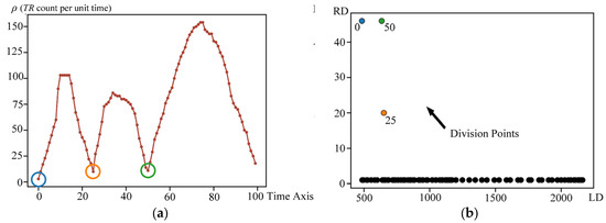
Figure 4.
Density time interval detection based on Dataset 1. (a) Trajectory temporal density; (b) decision graph. The points circled with different color circles in (a) correspond to the division points of different colors in (b).
In Dataset 1, we set the three-way threshold to 0.8 based on experimental results and conduct a series of ablation experiments on the proposed method. Initially, we compare the DTID-STFC method with clustering alone without DTID. Subsequently, we conduct experiments by utilizing DTID in conjunction with various classical clustering algorithms, including fuzzy c-means (DTID-SFC), spectral clustering (DTID-SC), ordering points to identify the clustering structure (DTID-OPTICS) [39], approximate neighbor propagation clustering (DTID-AP) [40], and hierarchical clustering (DTID-HC) [41]. Spectral clustering involves both spectral embedding and the k-means algorithm. For consistent result comparison, we assign trajectories to specific clusters based on the three-way membership grades obtained from STFC. Trajectories are assigned to the cluster that has the highest membership grade, while trajectories with ambiguous assignments across multiple clusters are labeled as noisy. The experiment outcomes are presented in Table 3.
Table 3.
Algorithm comparison in ablation experiments: bold values indicate optimal results.
Table 3 demonstrates that incorporating dense time interval detection before clustering (DTID-STFC) enhances the clustering accuracy compared to the method (STFC) without time interval calculation. On the other hand, hard clustering methods (SC, AP, and HC) may misclassify noisy trajectories into clusters, leading to lower accuracy in their results compared to STFC. STFC offers a more flexible membership grade representation compared to fuzzy clustering, enabling greater adaptability in handling noisy trajectories and trajectories with unclear boundaries. Compared to the density-based method OPTICS, STFC exhibits superior capability in handling simulated datasets.
We compare the DTID-STFC method with four trajectory clustering models: ST-DBSCAN [21], MTCA [16], MIF-STKNNDC [42], ISCM [30], and HDBSCAN-extended [22]. The results in Table 4 show that the DTID-STFC outperforms other state-of-the-art algorithms in Dataset 1 and has the shortest running time among the six models.
Table 4.
Performance evaluation of trajectory clustering models: bold values indicate optimal results.
ST-DBSCAN, MTCA, MIF-STKNNDC, and HDBSCAN-extended are extensions of density-based algorithms like DBSCAN and DPC. Density-based algorithms have inherent limitations when it comes to handling datasets with substantial variations in density. The DTID-STFC method utilizes spectral embedding to transform trajectories into a lower-dimensional space, enabling it to effectively handle datasets with various structures. By utilizing probabilistic assignments instead of deterministic ones, STFC enhances resilience against noise, resulting in superior performance compared to ISCM, which employs traditional spectral clustering.
The calculation of trajectory distances is often the most time-consuming step in trajectory clustering. Unlike other models that require calculating distances between all trajectories, the DTID-STFC method only needs to calculate distances between trajectories within the same time interval. As a result, compared to other methods, it demands less computation time, enabling higher efficiency in terms of computational workload. Our proposed method, which is based on spectral clustering, exhibits higher computational complexity compared to other models. This can be attributed to several steps inherent in the spectral clustering framework. Unlike density-based methods such as the complexity ST-DBSCAN, MTCA, and HDBSCAN, STFC involves computing the similarity matrix and subsequent eigen-decomposition, resulting in increased computational overhead. Despite the greater computational demands, it offers advantages in terms of clustering quality.
4.4. Experiment in Mesoscale Cyclonic Eddies Trajectory
Mesoscale eddies, especially mesoscale cyclonic eddies, have been shown to exhibit significant monsoonal seasonality [43,44] and high dynamicity [45] in the South China Sea, playing an important role in transporting heat, salt, and other oceanic properties. Therefore, it is appropriate to validate the proposed method by utilizing mesoscale cyclonic eddies’ trajectories in the South China Sea region.
We first construct the temporal distribution of trajectories (see Figure 5a) and corresponding decision graph (see Figure 5b) based on mesoscale cyclonic eddies. Based on Figure 5b, the dataset can be categorized into four dense time intervals: (11, 12, 1), (2–4), (5–7), and (8–10). The temporal density of trajectories within each time interval conforms to a Gaussian distribution.
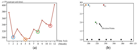
Figure 5.
Density time interval detection based on Dataset 2. (a) Trajectory temporal density; (b) decision graph. The points circled with different color circles in (a) correspond to the division points of different colors in (b).
As shown in Figure 5a, the density of eddy trajectories during (Nov–Jan.) is notably higher compared to other time intervals. This phenomenon can be attributed to the increased convective activity and temperature gradients [46], which promote the genesis of mesoscale cyclonic eddies during this period. On the other hand, the trajectory temporal density during (Feb.–April) and (May–Jul.) is lower due to the weaker summer monsoon winds [47] and the influence of typhoons. In contrast, (Aug.–Oct.) exhibits higher trajectory density. These findings reveal that the identified time intervals align with external environmental driving factors, further indicating the scientific interpretability of DTID.
Next, we apply STFC separately within each DTI and assess the normalized Silhouette Coefficient, DBI, and CHI values for various values. By examining the patterns of minimization and maximization in these three unsupervised metrics, we determine that the optimal value is consistently 4 for all , as shown in Figure 6.
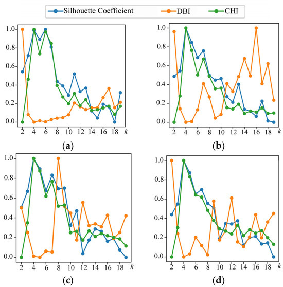
Figure 6.
The normalized Silhouette Coefficient, DBI, and CHI for different values of , , , and , corresponding to (a), (b), (c), and (d), respectively.
To further validate the advantages of the proposed method, we apply five diverse clustering algorithms (AP, HC, OPTICS, SC, and STFC) to cluster the trajectories for four dense time intervals. These trajectories are visualized by reducing their dimensions to two-dimensional data points using T-SNE [48], as shown in Figure 7. It is evident that STFC successfully groups the data points into intuitive and reasonable clusters, while the results from SC, AP, and HC exhibit unclear boundaries between clusters. As shown in Figure 7, it can be observed that the dataset lacks distinct high-density clusters, making it challenging to set appropriate density parameters for the OPTICS algorithm and difficult to identify suitable clusters.
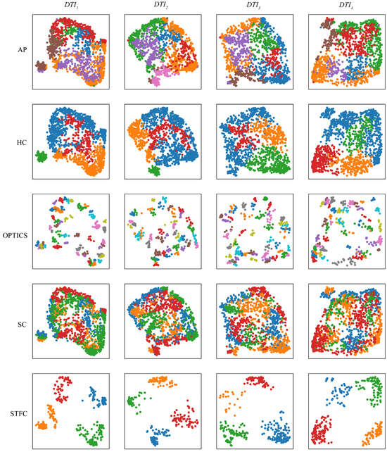
Figure 7.
T-SNE visualization clustering results. Each row shows the same algorithm, while each column shows the same time interval. Different colors represent different result clusters.
The spatial distribution of trajectory clusters in the STFC algorithm results is shown in Figure 8. It reveals significant spatial distributions among the trajectory clusters within each time period. Table 5 presents the average Pearson correlation coefficients [49] between attributes within each . Analyzing the table, we observe distinct movement patterns among the mesoscale cyclonic eddies in the South China Sea.
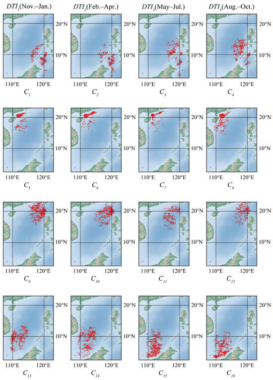
Figure 8.
Visualization of clustering results based on Dataset 2 in four dense time intervals. Each row shows the geographically proximate locations for clusters, and each column shows the same time interval.
Table 5.
The average Pearson correlation coefficients of clustering results.
In (Aug.–Oct.), the eddies in the southeastern region () tend to move northwest, which differs from the westward movement observed in other time intervals (–). The trajectories in the northwestern region (–) predominantly exhibit southwestward motion, with in (Nov.–Jan.) showing this trend prominently. The trajectories in the northeastern region () exhibit a more pronounced westward activity compared to other regions. In (May–Jul.), the northwest-moving behavior of these trajectories () is particularly evident during this time interval. The cyclonic eddies in the southwestern region (, ) move southwest from May to October, while during the remaining time, they (, ) predominantly drift in a west-northwest direction.
4.5. Experiment in AIS Vessel Trajectory
To better demonstrate the applicability of the proposed method to diverse oceanic trajectories, we conduct a thorough study and analysis using AIS vessel data. Based on the analysis presented in Section 3.1, we divide vessel routes into two dense time intervals: and , corresponding to the time frames of 10:00–21:00 and 22:00–09:00, respectively. Subsequently, we determine the optimal values of for and as 5, based on three metrics (CHI, Silhouette Coefficient, and DBI), as shown in Figure 9.
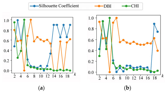
Figure 9.
The normalized Silhouette Coefficient, DBI, and CHI for different values of and , corresponding to (a) and (b), respectively.
We visualize the clustering results by reducing the trajectories within each to two-dimensional data points using various algorithms, as shown in Figure 10. The visualization results of STFC distinctly delineate different clusters compared to other methods, which exhibit mixed-color clusters. The figure illustrates that OPTICS struggles with non-uniform density data because it is challenging to set a uniform density parameter. On the other hand, AP, HC, and SC cluster all points (including potentially some noisy trajectories).
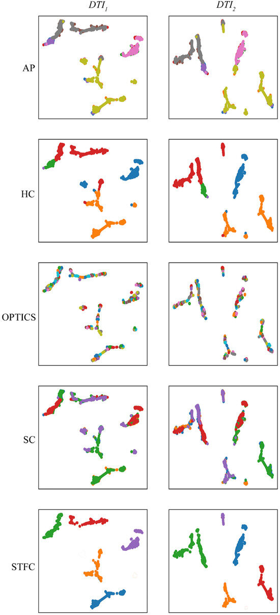
Figure 10.
T-SNE visualization clustering results. Each row shows the same algorithm, while each column shows the same time interval. Different colors represent different result clusters.
By computing the average Pearson correlation coefficients within trajectory clusters, we gain deeper insights into discerning the disparities among outcomes and identifying distinct movement patterns. From Table 6, it is evident that fishing vessels (, , , , and ) predominantly head eastward during (10:00–21:00), while (, , , , and ) they primarily navigate westward during (22:00–09:00). During , the fishing vessel (), located within the geographical range of 103.558°E–176.664°E, 6.850°S–36.217°N, exhibits a significant negative correlation between longitude and latitude changes, suggesting a tendency towards southeastward linear movement. During , vessels () within the geographic range of 10°W–114.327°W, 10.657°S–11.505°S predominantly travel in a southwestward linear trajectory.
Table 6.
The average Pearson correlation coefficients of clustering results.
4.6. Parameter Analysis
The proposed method involves two adjustable parameters, the time window size rate and the three-way threshold . The size of the time window adapts according to the time axis, with the range of set to [0.1, 0.2, 0.3, 0.4, 0.5]. The three-way membership grade primarily serves to enhance the judgment of membership grade, with parameter values ranging from [0.5, 0.6, 0.7, 0.8, 0.9, 1.0]. From Figure 11, it is clear that configuring parameters and within the ranges of 0.1–0.2 and 0.7–0.8, respectively, yields favorable outcomes on Dataset 1 and Dataset 2. Consequently, we opt to set the time window size rate and to 0.2 and 0.8, respectively, across all experiments.
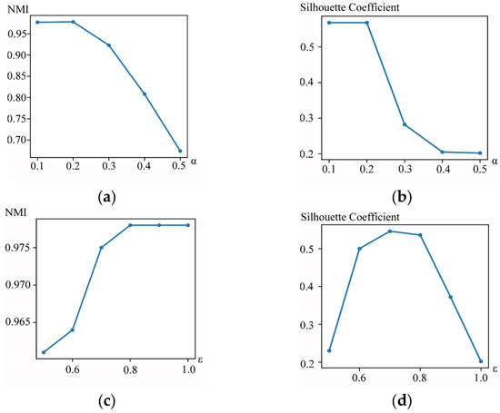
Figure 11.
Clustering performance of DTID-STFC with different parameter settings of the time window size rate and ε. (a) The NMI value with the change in the time window size rate on Dataset 1. (b) The silhouette coefficient value with the change in the time window size rate on Dataset 2. (c) The NMI value with the change in ε on Dataset 1. (d) The Silhouette Coefficient value with the change in the time window size rate on Dataset 2.
4.7. Convergence Experiments
We also conducted convergence experiments on the two datasets (Dataset 1 and Dataset 2) for the three-way fuzzy clustering algorithm and visualized the loss value with respect to the number of iterations. From Algorithm 1, it is evident that iterations in STFC continue until the three-way membership grade matrix converges. Hence, the loss value represents the difference between the matrix before and after iteration:
where represents the -norm of the matrix difference. The curves corresponding to the two datasets are shown in Figure 12 and Figure 13, respectively. These figures also demonstrate that loss decreases and converges to a stable value within 20 iterations. This validates the convergence of algorithm.
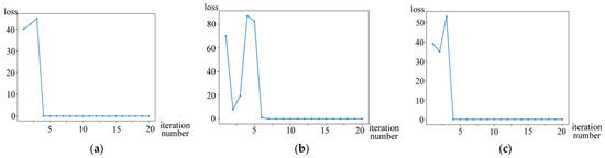
Figure 12.
The curve with respect to loss at each iteration of the proposed method on Dataset 1. (a), (b), and (c) correspond to , , and , respectively.
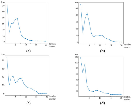
Figure 13.
The curve with respect to loss at each iteration of the proposed method on Dataset 2. (a), (b), (c), and (d) correspond to , , , and , respectively.
5. Discussion
Our method achieves higher accuracy than traditional approaches, allowing for more effective capture of periodic patterns in ocean trajectories and providing more precise clustering results. While our method yields satisfactory results, its higher computational demands require careful consideration in practical applications. Future research may focus on developing more efficient algorithms to mitigate computational burden while maintaining clustering performance. In parameter analysis experiments, we observed that the model is sensitive to parameter variations, highlighting the importance of setting appropriate parameters across datasets and scenarios. Additionally, our method demonstrates good convergence within datasets, effectively converging to global optimal solutions during the iterative process, enabling the rapid capture of latent patterns within ocean data.
From the clustering results, it is evident that our approach achieves significant results on two real datasets. In Dataset 2, we observe varying movement patterns of mesoscale eddies at different time intervals, indicating that our method successfully detects multiple periodic patterns or regularities in oceanic trajectories. In Dataset 3, distinct sailing patterns of vessel data at two different time intervals are identified, further validating the effectiveness and applicability of our method. These findings offer crucial insights for oceanographic research, aiding in a deeper understanding of patterns and trends in oceanic motion.
These results further validate our hypotheses: (1) oceanic trajectories exhibit evident periodic behaviors due to seasonal fluctuations in climatic variables; (2) these periodic patterns manifest differently within distinct time intervals; and (3) considering the temporal distributions of trajectories can provide deeper insights into the periodicities. This research lays the groundwork for more a comprehensive discovery of periodic behaviors embedded within complex spatiotemporal oceanic trajectory data. Coupling trajectory clustering with environmental data and machine learning holds potential to substantially advance our understanding of ocean processes.
6. Conclusions
We propose the DTID-STFC method to mine multiple periodic patterns from complex oceanic trajectories, which enhances our understanding of the temporal dynamics and general fluctuations of oceanic processes. We assess the performance of the DTID-STFC method on the simulated datasets using five common metrics and compare it with traditional algorithms and state-of-the-art trajectory clustering models. The results demonstrate that DTID-STFC accurately identifies dense time intervals and clusters within the simulated trajectories. Subsequently, we apply the DTID-STFC method to investigate the spatiotemporal trajectories of mesoscale cyclonic eddies in the South China Sea and visualize the results. This method successfully identifies four dense time intervals of eddy trajectories and clusters the trajectories within each time interval into more distinct clusters compared to four traditional algorithms, which align well with physical oceanographic processes. The analysis of mesoscale cyclonic eddies aids in discovering multiple periodic behaviors of mesoscale eddies over time, providing valuable insights into the study of these phenomena in the South China Sea. Finally, the DTIT-STFC method detects two dense time intervals from AIS data and clusters them separately. The results reveal distinctly different motion trends among vessels within two time intervals, with each exhibiting unique navigation patterns. This underscores the significance of temporal segmentation in understanding maritime vessel behaviors and highlights the necessity of time-aware analysis in maritime studies for comprehensive insights into vessel dynamics and operational patterns.
Additionally, similar periodic patterns may exist in other types of oceanic trajectory data. Applying the framework to trajectories of other marine species or regions would demonstrate the generalizability and scalability of the approach. Further investigation into multi-scale (e.g., hourly, daily, and monthly) periodicities could also reveal more intricate temporal dependencies.
Author Contributions
Conceptualization, validation, and writing—original draft preparation, Y.D. and K.C.; methodology, formal analysis, and visualization, K.C.; writing—review and editing, G.Y., W.Y. and Z.X.; supervision, W.S.; funding acquisition, Y.D. All authors have read and agreed to the published version of the manuscript.
Funding
This research was funded by the National Key Research and Development Program of China (No. 2021YFC3101602).
Data Availability Statement
The data supporting this research are openly available at www.aviso.altimetry.fr (accessed on 28 January 2024). For the experimental code of this paper, you can contact the author’s e-mail. E-mail: ckeqi97@gmail.com.
Acknowledgments
We would like to thank the anonymous reviewers for their insightful comments and substantial help in improving this paper. All authors have read and agreed to the published version of the manuscript.
Conflicts of Interest
The authors declare no conflict of interest.
References
- Cuenca-Jara, J.; Terroso-Saenz, F.; Valdés-Vela, M.; Skarmeta, A.F. Classification of spatio-temporal trajectories from volunteer geographic information through fuzzy rules. Appl. Soft Comput. 2020, 86, 105916. [Google Scholar] [CrossRef]
- Liu, W.; Wang, B.; Yang, Y.; Mou, N.; Zheng, Y.; Zhang, L.; Yang, T. Cluster analysis of microscopic spatio-temporal patterns of tourists’ movement behaviors in mountainous scenic areas using open GPS-trajectory data. Tour. Manag. 2022, 93, 104614. [Google Scholar] [CrossRef]
- Niu, X.; Zhu, J.; Wu, C.Q.; Wang, S. On a clustering-based mining approach for spatially and temporally integrated traffic sub-area division. Eng. Appl. Artif. Intell. 2020, 96, 103932. [Google Scholar] [CrossRef]
- Li, Z.; Yu, W.; Li, T.; Murty, V.S.N.; Tangang, F. Bimodal character of cyclone climatology in the Bay of Bengal modulated by monsoon seasonal cycle. J. Clim. 2013, 26, 1033–1046. [Google Scholar] [CrossRef]
- Ottesen, E.A.; Young, C.R.; Gifford, S.M.; Eppley, J.M.; Marin, R., III; Schuster, S.C.; DeLong, E.F. Multispecies diel transcriptional oscillations in open ocean heterotrophic bacterial assemblages. Science 2014, 345, 207–212. [Google Scholar] [CrossRef] [PubMed]
- Shankar, D.; Vinayachandran, P.N.; Unnikrishnan, A.S. The monsoon currents in the north Indian Ocean. Prog. Oceanogr. 2002, 52, 63–120. [Google Scholar] [CrossRef]
- Liu, Q.; Hou, Z.; Yang, J. Detecting Spatial Communities in Vehicle Movements by Combining Multi-Level Merging and Consensus Clustering. Remote Sens. 2022, 14, 4144. [Google Scholar] [CrossRef]
- Wan, Y.; Fei, Y.; Wu, T.; Jin, R.; Xiao, T. A Novel Impervious Surface Extraction Method Integrating POI, Vehicle Trajectories, and Satellite Imagery. IEEE J. Sel. Top. Appl. Earth Obs. Remote Sens. 2021, 14, 8804–8814. [Google Scholar] [CrossRef]
- Yang, Y.; Cai, J.; Yang, H.; Zhang, J.; Zhao, X. TAD: A trajectory clustering algorithm based on spatial-temporal density analysis. Expert Syst. Appl. 2020, 139, 112846. [Google Scholar] [CrossRef]
- Li, F.; Shi, W.; Zhang, H. A Two-Phase Clustering Approach for Urban Hotspot Detection with Spatiotemporal and Network Constraints. IEEE J. Sel. Top. Appl. Earth Obs. Remote Sens. 2021, 14, 3695–3705. [Google Scholar] [CrossRef]
- Lee, J.G.; Han, J.; Whang, K.Y. Trajectory clustering: A partition-and-group framework. In Proceedings of the 2007 ACM SIGMOD International Conference on Management of Data, Beijing, China, 11–14 June 2007. [Google Scholar] [CrossRef]
- Tang, C.; Chen, M.; Zhao, J.; Liu, T.; Liu, K.; Yan, H.; Xiao, Y. A novel ship trajectory clustering method for Finding Overall and Local Features of Ship Trajectories. Ocean Eng. 2021, 241, 110108. [Google Scholar] [CrossRef]
- Qiao, D.; Yang, X.; Liang, Y.; Hao, X. Rapid trajectory clustering based on neighbor spatial analysis. Pattern Recognit. Lett. 2022, 156, 167–173. [Google Scholar] [CrossRef]
- Ansari, M.Y.; Ahmad, A.; Bhushan, G. Spatiotemporal trajectory clustering: A clustering algorithm for spatiotemporal data. Expert Syst. Appl. 2021, 178, 115048. [Google Scholar] [CrossRef]
- Bermingham, L.; Lee, I. A general methodology for n-dimensional trajectory clustering. Expert Syst. Appl. 2015, 42, 7573–7581. [Google Scholar] [CrossRef]
- Pan, X.; He, Y.; Wang, H.; Xiong, W.; Peng, X. Mining regular behaviors based on multidimensional trajectories. Expert Syst. Appl. 2016, 66, 106–113. [Google Scholar] [CrossRef]
- Hong, Z.; Chen, Y.; Mahmassani, H.S. Recognizing network trip patterns using a spatio-temporal vehicle trajectory clustering algorithm. IEEE Trans. Intell. Transp. Syst. 2017, 19, 2548–2557. [Google Scholar] [CrossRef]
- Shi, Y.; Wang, D.; Wang, X.; Chen, B.; Ding, C.; Gao, S. Sensing Travel Source–Sink Spatiotemporal Ranges Using Dockless Bicycle Trajectory via Density-Based Adaptive Clustering. Remote Sens. 2023, 15, 3874. [Google Scholar] [CrossRef]
- Zhang, D.; Zhang, Y.; Zhang, C. Data mining approach for automatic ship-route design for coastal seas using AIS trajectory clustering analysis. Ocean Eng. 2021, 236, 109535. [Google Scholar] [CrossRef]
- Yang, J.; Liu, Y.; Ma, L.; Ji, C. Maritime traffic flow clustering analysis by density based trajectory clustering with noise. Ocean Eng. 2022, 249, 111001. [Google Scholar] [CrossRef]
- Birant, D.; Kut, A. ST-DBSCAN: An algorithm for clustering spatial–temporal data. Data Knowl. Eng. 2007, 60, 208–221. [Google Scholar] [CrossRef]
- Wang, L.; Chen, P.; Chen, L.; Mou, J. Ship AIS trajectory clustering: An HDBSCAN-based approach. J. Mar. Sci. Eng. 2021, 9, 566. [Google Scholar] [CrossRef]
- Von Luxburg, U. A tutorial on spectral clustering. Stat. Comput. 2007, 17, 395–416. [Google Scholar] [CrossRef]
- Bezdek, J.C.; Ehrlich, R.; Full, W. FCM: The fuzzy c-means clustering algorithm. Comput. Geosci. 1984, 10, 191–203. [Google Scholar] [CrossRef]
- Deng, C.; Choi, H.C.; Park, H.; Hwang, I. Trajectory pattern identification and classification for real-time air traffic applications in Area Navigation terminal airspace. Transp. Res. Part C Emerg. Technol. 2022, 142, 103765. [Google Scholar] [CrossRef]
- Liu, G.; Fan, Y.; Zhang, J.; Wen, P.; Lyu, Z.; Yuan, X. Deep flight track clustering based on spatial-temporal distance and denoising auto-encoding. Expert Syst. Appl. 2022, 198, 116733. [Google Scholar] [CrossRef]
- Rodriguez, A.; Laio, A. Clustering by fast search and find of density peaks. Science 2014, 344, 1492–1496. [Google Scholar] [CrossRef] [PubMed]
- Anonymized AIS Training Data, Distributed by Global Fishing Watch, May 2020. Available online: https://globalfishingwatch.org/data-download/datasets/public-training-data-v1 (accessed on 28 January 2024).
- Taylor, J.; Zhou, X.; Rouphail, N.M.; Porter, R.J. Method for investigating intradriver heterogeneity using vehicle trajectory data: A dynamic time warping approach. Transp. Res. Part B Methodol. 2015, 73, 59–80. [Google Scholar] [CrossRef]
- Li, H.; Lam, J.S.L.; Yang, Z.; Liu, J.; Liu, R.W.; Liang, M.; Li, Y. Unsupervised hierarchical methodology of maritime traffic pattern extraction for knowledge discovery. Transp. Res. Part C Emerg. Technol. 2022, 143, 103856. [Google Scholar] [CrossRef]
- Yao, Y. Three-way decisions with probabilistic rough sets. Inf. Sci. 2010, 180, 341–353. [Google Scholar] [CrossRef]
- Piciarelli, C.; Micheloni, C.; Foresti, G.L. Trajectory-based anomalous event detection. IEEE Trans. Circuits Syst. Video Technol. 2008, 18, 1544–1554. [Google Scholar] [CrossRef]
- Mesoscale Eddy Trajectory Atlas META3.2 Delayed-Time All Satellites: Version META3.2 DT Allsat; AVISO: Redwood City, CA, USA, 2022. [CrossRef]
- Strehl, A.; Ghosh, J. Cluster ensembles—A knowledge reuse framework for combining multiple partitions. J. Mach. Learn. Res. 2002, 3, 583–617. [Google Scholar]
- Chacón, J.E.; Rastrojo, A.I. Minimum adjusted Rand index for two clusterings of a given size. Adv. Data Anal. Classif. 2023, 17, 125–133. [Google Scholar] [CrossRef]
- Caliński, T.; Harabasz, J. A dendrite method for cluster analysis. Commun. Stat. Theory Methods 1974, 3, 1–27. [Google Scholar] [CrossRef]
- Rousseeuw, P.J. Silhouettes: A graphical aid to the interpretation and validation of cluster analysis. J. Comput. Appl. Math. 1987, 20, 53–65. [Google Scholar] [CrossRef]
- Davies, D.L.; Bouldin, D.W. A cluster separation measure. IEEE Trans. Pattern Anal. Mach. Intell. 1979, PAMI-1, 224–227. [Google Scholar] [CrossRef]
- Ankerst, M.; Breunig, M.M.; Kriegel, H.P.; Sander, J. OPTICS: Ordering points to identify the clustering structure. ACM Sigmod Rec. 1999, 28, 49–60. [Google Scholar] [CrossRef]
- Frey, B.J.; Dueck, D. Clustering by passing messages between data points. Science 2007, 315, 972–976. [Google Scholar] [CrossRef]
- Murtagh, F.; Legendre, P. Ward’s hierarchical agglomerative clustering method: Which algorithms implement Ward’s criterion? J. Classif. 2014, 31, 274–295. [Google Scholar] [CrossRef]
- Jiang, Q.; Yu, L.I.U.; Ziran DI, N.G.; Shun SU, N. Behavior pattern mining based on spatiotemporal trajectory multidimensional information fusion. Chin. J. Aeronaut. 2023, 36, 387–399. [Google Scholar] [CrossRef]
- Gulakaram, V.S.; Vissa, N.K.; Bhaskaran, P.K. Role of mesoscale eddies on atmospheric convection during summer monsoon season over the Bay of Bengal: A case study. J. Ocean Eng. Sci. 2018, 3, 343–354. [Google Scholar] [CrossRef]
- Li, H.; Wiesner, M.G.; Chen, J.; Ling, Z.; Zhang, J.; Ran, L. Long-term variation of mesopelagic biogenic flux in the central South China Sea: Impact of monsoonal seasonality and mesoscale eddy. Deep Sea Res. Part I Oceanogr. Res. Pap. 2017, 126, 62–72. [Google Scholar] [CrossRef]
- Du, Y.; Liu, Q.; Wang, L.; Xu, X.; Wei, Q.; Song, W. Multi-scale rotating anchor mechanism based automatic detection of ocean mesoscale eddy. J. Image Graph. 2022, 27, 3092–3101. [Google Scholar]
- Islam, M.M.; Sado, K. Time series analysis of SST for Java Sea and South China Sea using NOAA AVHRR data. In Proceedings of the 34th Conference of Remote Sensing Society of Japan, Tokyo, Japan, 1 November 2003. [Google Scholar]
- Tang, H.; Micheels, A.; Eronen, J.; Fortelius, M. Regional climate model experiments to investigate the Asian monsoon in the Late Miocene. Clim. Past 2011, 7, 847–868. [Google Scholar] [CrossRef]
- Van Der Maaten, L. Accelerating t-SNE using tree-based algorithms. J. Mach. Learn. Res. 2014, 15, 3221–3245. [Google Scholar]
- Pearson, K.V.I.I. Note on regression and inheritance in the case of two parents. Proc. R. Soc. Lond. 1895, 58, 240–242. [Google Scholar] [CrossRef]
Disclaimer/Publisher’s Note: The statements, opinions and data contained in all publications are solely those of the individual author(s) and contributor(s) and not of MDPI and/or the editor(s). MDPI and/or the editor(s) disclaim responsibility for any injury to people or property resulting from any ideas, methods, instructions or products referred to in the content. |
© 2024 by the authors. Licensee MDPI, Basel, Switzerland. This article is an open access article distributed under the terms and conditions of the Creative Commons Attribution (CC BY) license (https://creativecommons.org/licenses/by/4.0/).