A WebGIS-Based System for Supporting Saline–Alkali Soil Ecological Monitoring: A Case Study in Yellow River Delta, China

Abstract

Monitoring and evaluation of soil ecological environments are very important to ensure saline–alkali soil health and the safety of agricultural products. It is of foremost importance to, within a regional ecological risk-reduction strategy, develop a useful online system for soil ecological assessment and prediction to prevent people from suffering the threat of sudden disasters. However, the traditional manual or empirical parameter adjustment causes the mismatch of the hyperparameters of the model, which cannot meet the urgent need for high-performance prediction of soil properties using multi-dimensional data in the WebGIS system. To this end, this study aims to develop a saline–alkali soil ecological monitoring system for real-time monitoring of soil ecology in the Yellow River Delta, China. The system applied advanced web-based GIS, including front-end and back-end technology stack, cross-platform deployment of machine learning models, and a database embedded in multi-source environmental variables. The system adopts a five-layer architecture and integrates functions such as data statistical analysis, soil health assessment, soil salt prediction, and data management. The system visually displays the statistical results of air quality, vegetation index, and soil properties in the study area. It provides users with ecological risk assessment functions to analyze heavy metal pollution in the soil. Specially, the system introduces a tree-structured Parzan estimator (TPE)-optimized machine learning model to achieve accurate prediction of soil salinity. The TPE–RF model had the highest prediction accuracy (R² = 94.48%) in the testing set in comparison with the TPE–GBDT model, which exhibited a strong nonlinear relationship between environmental variables and soil salinity. The system developed in this study can provide accurate saline–alkali soil information and health assessment results for government agencies and farmers, which is of great significance for agricultural production and saline–alkali soil ecological protection.

1. Introduction

Saline–alkali land is an important reserve cultivated land resource, and it is an important buffer zone for global environmental change [1]. Saline–alkali soil health is not only a critical foundation for sustaining global ecosystems and agricultural development [2,3], but also plays an important role in ensuring food security, maintaining biodiversity, and promoting sustainable development [4,5,6]. In recent years, with the acceleration of urbanization, the decline in soil quality (such as soil salinization and heavy metal accumulation) has become an important threat to saline–alkali soil health [7,8]. For example, heavy metals in soil can cause problems such as farmland soil degradation and pollution by changing soil physical and chemical properties [9], posing a threat to the quality of agricultural products and human health [10]. The prevention and early warning of saline–alkali soil health based on Geographic Information System (GIS) has been widely used. It has the advantages of map data processing, spatial analysis, and visualization, and can effectively detect the spatial distribution of regional soil properties [11,12]. However, the traditional GIS technology cannot achieve real-time monitoring and evaluation of saline–alkali soil ecological health and has a lag for the prevention and control of saline–alkali soil health risks. The information technology represented by WebGIS is emerging, gradually applying to many fields such as agriculture, soil science, meteorology, and ecological protection [13,14,15,16]. Compared with traditional GIS, WebGIS enables real-time interaction for spatial data analysis, multiple functional services, and monitoring models [17,18]. Therefore, it is of great significance to develop a WebGIS system for saline–alkali soil ecological monitoring with integrated prediction and evaluation, which can improve the quality and efficiency of agricultural production and ensure the quality and safety of food.

At present, the development technology innovation of the WebGIS system can be divided into two types: database and evaluation model. The use of database technology in the WebGIS system can achieve efficient storage, management, and analysis of geographic information data. For example, the Geo APEXOL interface was applied to the WebGIS system for the evaluation of nonpoint source pollution on-site [19]. The interface used a complete database of soil, meteorology, land use, DEM, and agricultural management, which realized the automation of the model establishment process [19]. Cao et al. used B/S three-layer architecture, Oracle, and AJAX technology to build a database of trace elements in coal, and integrated WebGIS technology to realize the visualization of data and analysis of trace elements [20]. The monitoring of soil properties needs data such as topography, climate, vegetation, and remote sensing images, and a reliable database can efficiently manage these multi-source heterogeneous data.

The accurate evaluation model is the basis for the WebGIS system to accurately predict and evaluate the monitoring target, and the most commonly used model is the linear model. Yong et al. integrated the exponential smoothing prediction model into the WebGIS-based system to better fit the variation in heavy metal pollution in the soil [15]. The physics-based STONE model was used in the WebGIS system, which associated the potential rockfall source information with the earthquake-induced peak ground acceleration (PGA) scenario to simulate the earthquake-induced rockfall trajectory [21]. In addition, other linear models such as probability sampling [22] and curve fitting [23] were also applied to the WebGIS disaster monitoring system and combined with physical models to achieve real-time monitoring of landslides and typhoons [24,25]. Because the linear model has the advantages of a simple, easy-to-use, and stable fitting relationship, the WebGIS system embedded in the linear model can quickly monitor the target in real time. However, there is a significant nonlinear relationship between environmental variables and monitoring targets, resulting in low prediction accuracy of linear models, which cannot meet the high-precision evaluation of soil properties by the WebGIS system.

Obviously, compared with the linear model, a machine learning model has higher accuracy in evaluating soil properties [26]. According to our knowledge, the research on embedding machine learning models into WebGIS systems to monitor soil properties has not been reported, but many traditional studies have used machine learning models to predict soil properties. For example, Xiao et al. used random forest (RF), support vector machine (SVM), and extreme gradient boosting (XGB) models to predict soil salinity parameters [27]. They found that the overall performance of the XGB model was better than those of the SVM and RF models [27]. RF and Cubist models were used to predict the content of heavy metals in soil, and the RF model has higher accuracy in predicting Ni and Cu in comparison with the Cubist model [28]. Liu et al. compared the performance of random forest (RF), partial least squares regression (PLSR), support vector machine regression (SVMR), and Gaussian process regression (GPR) models in predicting soil water content (SWC), and proved that the GPR model has the best performance [29].

A high-performance machine learning model is the core of accurate real-time prediction of soil properties, which is in line with the future research trend of the WebGIS system. Although the choice of model is very important for the WebGIS system to predict soil properties online, many studies have found that the low performance and prediction accuracy of the model are essentially caused by the mismatch of hyperparameters of the model [30,31,32,33]. However, there is a key shortcoming in traditional machine learning to predict soil properties, which requires manual or empirical adjustment of hyperparameters. That is, hyperparameters can significantly affect the final performance of machine learning models [34,35,36]. For example, the hyperparameters of the GBDT model are divided into structural parameters and regularization parameters. The structural parameters are used to control the complexity and prediction accuracy of the model, including max_depth (specify the maximum depth of each tree), max_features (limit the number of features considered when branching the tree), and n_estimations (specifies the number of iterations, the number of trees). The regularization parameter is used to adjust the over-fitting phenomenon of the model, including min_impurity_decrease (limit the amount of information gain when splitting nodes), and reg_alpha (specify the proportion of subsampling in the modeling process) [37]. When the hyperparameter space of the prediction model is large, these hyperparameters interfere with each other. Manual parameter tuning leads to long, time-consuming, and low efficiency in finding hyperparameters, and it is difficult to find the optimal hyperparameters. Quickly finding the optimal combination of hyperparameters is the key to improving the prediction performance and accuracy of the model in the WebGIS system.

With the development of information technology, more and more optimization algorithms for machine learning hyperparameters are applied. For example, Yu et al. used the TPE algorithm to optimize the hyperparameters of the CatBoost model, constructed the TPE–CatBoost soil moisture spatial estimation model, and proved that the TPE–CatBoost model has high estimation accuracy [38]. Compared with traditional hyper-parameter tuning methods such as manual parameter tuning, grid search (GS), and random grid search (RGS), the TPE algorithm has the ability of parameter adaptive adjustment and global exploration and can search parameters in the entire parameter space [39]. Before reaching the global optimal value in the search space, it avoids falling into the local optimum [38], which significantly improves the accuracy of machine learning prediction. In order to meet the needs of the WebGIS system to deal with massive multi-source heterogeneous data, high-performance algorithms embedded in hyper-parameter optimization will be the inevitable requirement for achieving high-precision prediction and processing multi-dimensional data. However, to our knowledge, the application of a TPE-optimized machine learning model to the WebGIS monitoring system has not been reported. Specifically, whether WebGIS development technologies such as predictive model markup language (PMML) and Java-PMML (JPMML) can achieve cross-platform deployment of TPE-optimized machine learning models and encapsulate the deployed models without retraining and reloading to enhance the modular application flexibility and scalability of the core models. Furthermore, whether the TPE-optimized machine learning model can give full play to its best performance and optimal prediction accuracy in the WebGIS system is also not clear.

Therefore, the aim of this study is to develop a saline–alkali soil ecological monitoring system based on WebGIS technology in the Yellow River Delta of China, including a presentation layer, application layer, data analysis layer, application support layer, and database layer. The system provides the functions of soil statistical analysis, soil health evaluation, soil salinity prediction, and data management. The machine learning model optimized by TPE is embedded in the system, and the prediction accuracy of soil salinity is improved by combining vegetation index and air quality variables. The purpose of this study is to provide technical and application support for promoting sustainable agricultural development and saline–alkali soil ecological protection in the area.

2. Materials and Methods

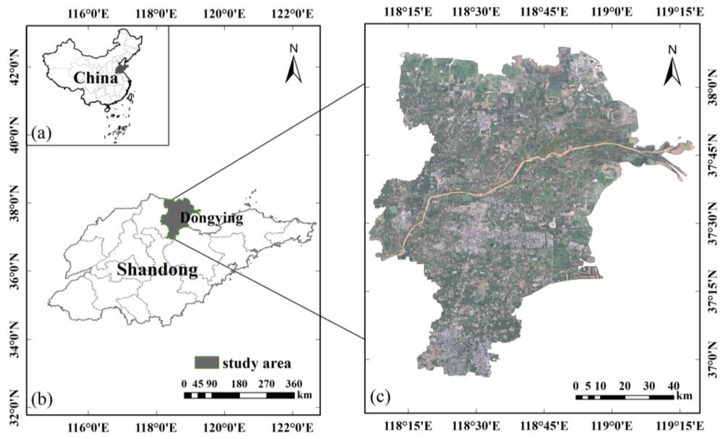
2.1. Study Area

The study area is located in the Yellow River Delta (YRD) of Shandong Province, China (Figure 1). It is an alluvial plain formed by sediment deposited in the Bohai depression at the mouth of the Yellow River. The study area is in the mid-latitude warm temperate zone and has a warm temperate continental monsoon climate with an average annual temperature of 14.2 °C and annual precipitation of 794 mm. The topography of the study area is flat, the parent material of the soil is loess alluvium, and the soil is rich in organic matter and nutrients, which provide good conditions for agricultural production. The region has developed agricultural production, with the main crop types being rice, wheat, and maize, and is rich in biodiversity. The area has a long history of oil extraction, fragile soil ecosystems, and severe salinization problems. Therefore, the monitoring of the soil ecological environment is crucial for the sustainable development of saline–alkali in this area.

2.2. Requirement Analysis

The Yellow River Delta is the location of the Chinese Shengli Oilfield, with a history of more than 60 years of oil exploitation. Human activities such as oil mining and smelting have caused great damage to the soil ecology in the region. The area is also a typical coastal saline–alkali land, and the ecological environment of farmland soil is very complex. This puts forward an urgent need for the monitoring and evaluation of the saline–alkali soil ecological environment. The monitoring of the ecological environment of saline–alkali soil in the YRD meets the national ecological protection strategic requirements. The Ministry of Ecology and Environment of China issued the “14th Five-Year Plan for Ecological and Environmental Monitoring” (28 December 2021), which pointed out that it is necessary to implement the environmental quality monitoring network construction project, improve the environmental quality monitoring and early warning capacity, strengthen the water ecological environment monitoring capacity in the Yellow River Basin, and give priority to supporting the ecological monitoring of national nature reserves such as the YRD. In addition, farmers and agricultural management departments need to understand farmland soil information and monitor soil ecological environment in real time for agricultural production and land use in the Yellow River Delta. Although some scholars have carried out research on farmland soil ecological monitoring in the Yellow River Delta region, such as providing solutions for soil improvement and water and salt regulation, there is still a lack of a complete ecological monitoring system as technical support or auxiliary measures. Therefore, this study developed a WebGIS-based saline–alkali soil ecology monitoring system to meet the urgent needs of various users for real-time monitoring of soil salinization and pollution risk prevention and control in the YRD.

2.3. Data Collection and Processing

2.3.1. Remote Sensing Data

In order to fully cover the scope of the study area, we selected two remote sensing images from the Sentinel-2 satellite (L2A level) in the same transit time (23 September 2022), which were obtained from the data sharing website of the European Space Agency (https://dataspace.copernicus.eu/, accessed on 12 November 2022). We used ENVI 5.3 software to preprocess the 11 bands (B1–B11) of Sentinel-2 image data, including band combination, mosaic cropping, and image mosaic, with a resolution set to 10 m × 10 m. Figure 2 shows eight soil texture feature statistics obtained by gray-level co-occurrence matrix (GLCM) processing, including Mean, Variance (VAR), Homogeneity (HOM), Contrast (CTRA), Difference (DIS), Entropy (ENT), Second-Order Moment (SECM), and Correlation (CORR). Four vegetation indices were obtained using the band calculation tool in the ENVI 5.3 software (Figure 2), including the Modified Normalized Difference Vegetation Index (MNDVI), Normalized Difference Vegetation Index (NDVI), Optimized Soil Regulated Vegetation Index (OSAVI), and Plant Senescence Reflectance Index (PSRI). The calculation formula for the vegetation index is shown in

Table 1. The formulae for vegetation indices based on Sentinel-2 remote sensing images.

Index	Formula		Reference
MNDVI	$(B7-B4)/(B7+B4)$	(1)	[40]
NDVI	$(B8-B4)/(B8+B4)$	(2)	[41]
OSAVI	$(1+0.16)\text{×}(B6-B5)/(B6+B5+0.16)$	(3)	[42]
PSRI	$(B4-B3)/B6$	(4)	[43]

.

2.3.2. Air Quality Data

Six air quality factors were selected as environmental variables, namely, CO, NO₂, O₃, SO₂, PM_2.5, and PM₁₀. The data came from the Dongying Municipal Environmental Protection Bureau (http://sthj.dongying.gov.cn/, accessed on 10 November 2022), including 40 air quality monitoring stations. We employed ordinary kriging (OK) to spatially interpolate the air quality factors of the 40 monitoring stations (Figure 3) in the ArcGIS 10.8 software and obtained raster data on air quality at a resolution of 10 m × 10 m.

2.3.3. Data on Soil Properties

In the last ten days of September 2022, a total of 60 soil samples were collected 0–20 cm from the surface at each sampling point in the study area. These samples were used to determine soil salinity, pH, and heavy metal content.

(1)

Soil salinity was determined using the quality method.

After the collected soil samples were pre-treated by removing impurities, air-dried indoors, and ground, they were mixed with water at a 1:5 soil-to-water ratio and shaken. The soil–water mixture was then filtered and the leachate was extracted with a large-bellied pipette, placed in a beaker, and heated in a water bath. A small amount of 15% H₂O₂ was added to remove organic matter and then evaporated. The beaker was dried in an oven at 105 °C for 4 h, cooled, and weighed with an analytical balance to measure the residue mass. The beaker was further dried in the oven for 2 h and then weighed until it reached a constant weight. The total amount of soluble salts (Equation (5)) was calculated as follows:

Total soluble salts = (m1 − m2)/m × 100

(5)

where the total soluble salt represents the mass fraction of soluble salt in the soil, m1 is the sum of the beaker and salt mass, m2 is the mass of the empty beaker, and m is the mass of the sample with the same volume of extracted liquid from the absorbed water.

(2)

The soil pH value was determined using the potentiometric method.

We weighed 10 g of air-dried soil sample, passed it through a 2 mm sieve into a beaker, and added 25 mL of carbon dioxide-free water or calcium chloride solution. We then stirred the solution with a glass rod, let it stand for 30 min, measured it with a pH meter, and recorded the pH value of the solution once the reading was stable. Figure 4 shows the interpolation results of soil pH and soil salinity obtained via ArcGIS processing.

(3)

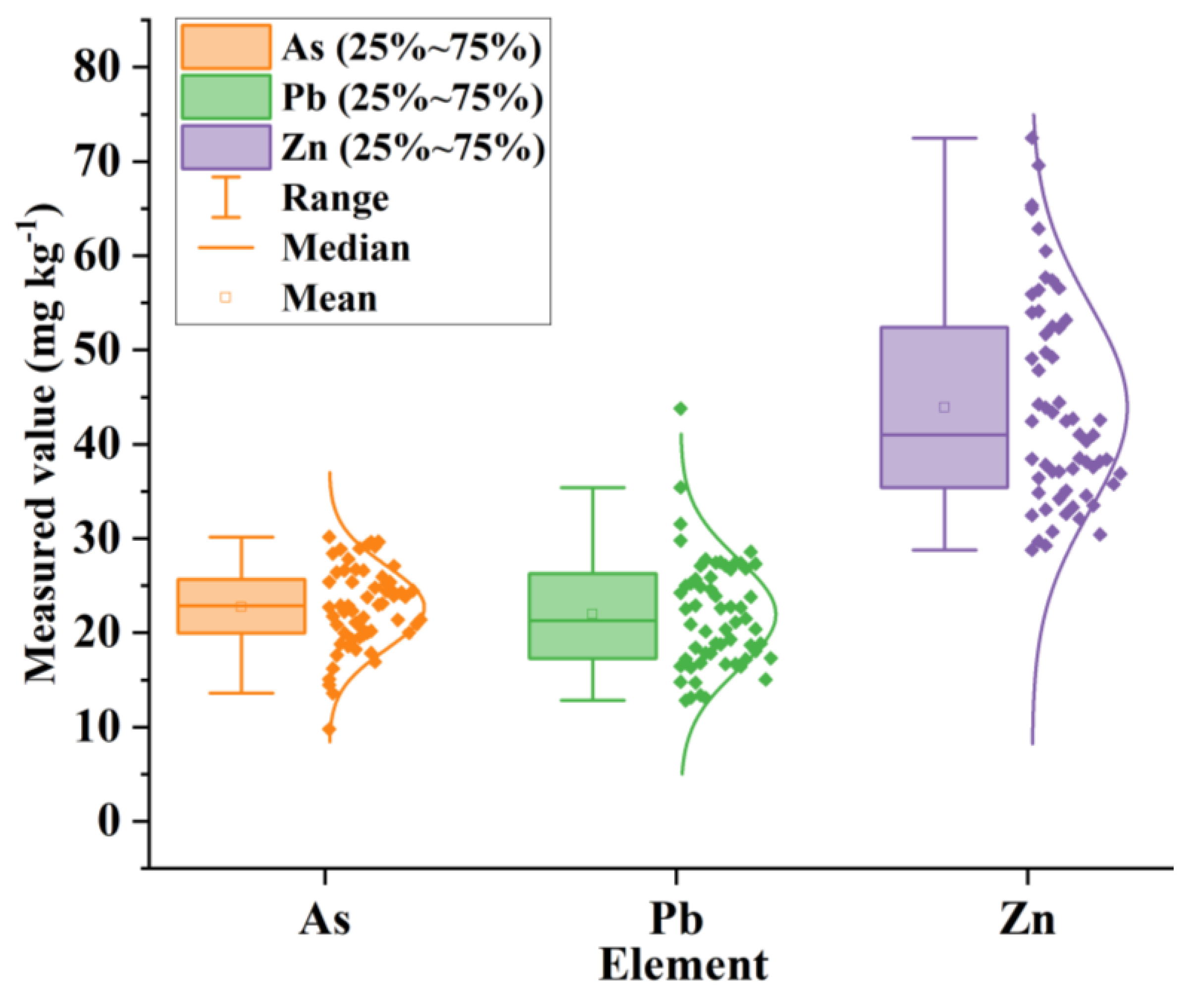
Determination of the heavy metal content in soil.

Soil was sampled from 4–6 points in each field, mixed, and packed into sample bags, and the coordinates of the sampling points were determined by high-precision GPS. The soil samples were brought back to the laboratory for natural air drying, removal of debris, crushing, grinding, and other pretreatments, and then passed through a 200-mesh nylon sieve. We weighed 0.2 g of soil sample, added 6 mL of HNO₃, 2 mL of HCl, and 2 mL of HF in a 3:1:1 ratio in a fume hood, and repeated all operations in parallel 3 times. The samples were placed in a microwave (CEM MARS5, NC, USA) for digestion, adding one GSS-1 standard soil sample and one blank to each batch. The measured contents of three heavy metals—As, Pb, and Zn—were measured using an inductively coupled plasma mass spectrometer (Agilent ICP-MS 7800, SC, CA, USA). Figure 5 shows the numerical distribution of heavy metal concentrations in the soil in the study area. As and Pb show normal distributions, while the median and mean values of Zn are quite different, resulting in non-normal characteristics.

2.4. Risk Assessment of Heavy Metals in Soil

The risk assessment of heavy metals in saline–alkali soil is crucial for the protection of farmland ecology. This study utilized three methods to evaluate heavy metals in soils: Single pollution index, Nemero comprehensive pollution index, and Hakanson potential ecological hazard index.

2.4.1. Single Pollution Index

The single pollution index model is used to evaluate the risk of a single heavy metal element in farmland soil [44], and the main heavy metal pollutants and their degrees of pollution can be determined. The calculation formula (Equation (6)) is as follows:

$$P_i=\frac{C_i}{S_i}$$

(6)

where $C_i$ (mg kg⁻¹) is the measured content of the i-th heavy metal in soil, $S_i$ (mg kg⁻¹) is the risk assessment standard threshold of the i-th heavy metal, and $P_i$ is the single factor index value of the i-th heavy metal element in the soil. The soil-based heavy metal standard used in this study is based on the Soil Environmental Quality and Risk Control Standard for Soil Contamination of Agricultural Land (GB 15618-2018) (https://www.mee.gov.cn/ (accessed on 7 April 2024)), which was published by the Ministry of Ecology and Environment of the People’s Republic of China.

2.4.2. Nemero Comprehensive Pollution Index

The Nemero comprehensive pollution index can comprehensively reflect the cumulative risk of multiple heavy metals at a single sampling point [45]. The calculation formula (Equation (7)) is as follows:

$$P_{total}=\sqrt{\frac{{(P_i)}^2+{(P_{i\max })}^2}{2}}$$

(7)

where $P_{total}$ is the Nemero comprehensive pollution index value of various heavy metals at soil sampling points and $P_{i\max }$ is the maximum value of the single factor index of each heavy metal element in the soil sampling point. The Nemero comprehensive pollution index is divided into five grades, and the evaluation results are shown in

Table 2. Evaluation level of the Nemero comprehensive pollution index.

Grade	Range	Grade Division	Explanation
1	PTotal ≤ 0.7	Safety	Clean level, crop healthy.
2	0.7 < PTotal ≤ 1	Warning level	Critical cleaning, limited use.
3	1 < PTotal ≤ 2	Light pollution	Slight pollution, crops are at risk.
4	2 < PTotal ≤ 3	Moderate pollution	Moderate pollution, crop risk is high.
5	PTotal > 3	Heavy pollution	Heavy pollution, crop risk is extremely high.

.

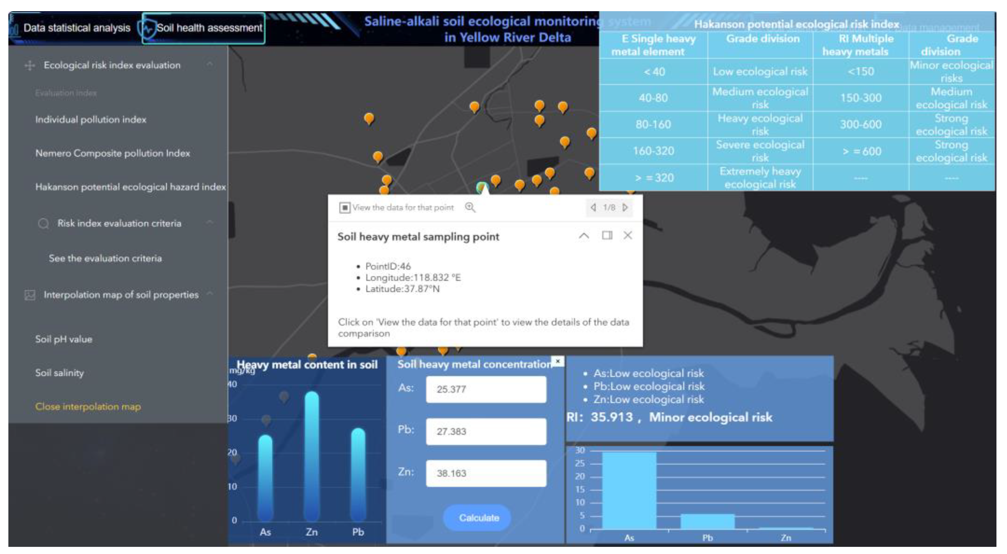
2.4.3. Hakanson Potential Ecological Risk Index

The potential ecological risk index is a risk assessment method for heavy metals in farmland soil [46] that considers the toxicological properties of each heavy metal, the degree of pollution of the soil, and the comprehensive ecological risk. The calculation process (Equations (8)–(10)) is as follows:

$$C_f^i=\frac{C^i}{C_n^i}$$

(8)

where $C^i$ is the measured value of the concentration of the i-th heavy metal element (mg kg⁻¹), $C_n^i$ is the evaluation reference value of the i-th heavy metal element in saline–alkali soil, and $C_f^i$ is the pollution coefficient of a single element.

$$E_r^i=T_r^i\times C_f^i$$

(9)

where $T_r^i$ is the toxicity response coefficient of the i-th heavy metal and $E_r^i$ is the potential ecological risk index of a single i-th heavy metal element. The toxicity coefficient of the potential ecological risk index of heavy metals is given in

Table 3. Toxicity coefficient of the Hakanson potential ecological hazard index.

Heavy Metal	As	Pb	Zn	Total
Toxicity coefficient	10	5	1	-

.

$$RI={\displaystyle \sum _{i=1}^m{E}_r^i}$$

(10)

RI represents the potential ecological risk index of various heavy metals in saline–alkali soil, and the evaluation results of the potential ecological risk index of heavy metals are divided into five levels (

Table 4. Evaluation level of the Hakanson potential ecological hazard index.

${\mathit{E}}_{\mathit{r}}^{\mathit{i}}$	Grade Division	RI	Grade Division
<40	Low ecological risk	<150	Slight ecological risks
40–80	Medium ecological risk	150–300	Medium ecological risk
80–160	Heavy ecological risk	300–600	Strong ecological risks
160–320	Severe ecological risk	≥600	Extremely strong ecological risk
≥320	Extremely heavy ecological risk	-	-

).

2.5. System Architecture

The system adopts a five-layer architecture, including the presentation layer, application layer, data analysis layer, application support layer, and database layer (Figure 6). Each module interacts with each other through the interface and realizes the functions of data statistical analysis, soil health assessment, soil salinity prediction, and data management. The system architecture is based on a front-end technology stack (Vue.js, Element UI, Node.js, Axios, and Echarts.js), back-end technology stack (Spring Boot and Mybatis-Plus), cross-platform deployment of machine learning models (Predictive Model Markup Language (PMML), Java PMML), and the MySQL database. The choice of these development tools and technologies can improve development efficiency and system performance, making the system have a good user interface, reliable back-end logic, efficient data interaction, and scalable machine learning capabilities.

2.5.1. Performance Layer

The presentation layer is the front end of the system, which consists of the user interface. In this study, Vue.js, Element UI, and Echarts.js technologies were used for front-end development, and Node.js was used as the server-running environment. Vue.js is a popular JavaScript framework that can add libraries according to user needs for building visual interactive interfaces [47]. Element UI is a desktop UI component library based on Vue.js, providing a wealth of components and templates to meet the needs of developers for interface design. Echarts.js is an open-source JavaScript-based visualization library for creating interactive data visualization charts [48]. We used Axios for front-end data interaction and Webpack for packaging. Axios is a promise-based HTTP client that automatically transforms the data format of requests and responses, simplifying the coding of data processing. In the presentation layer of this system, the Vue.js framework is used to build the front-end user interface to realize data visualization and components and templates provided by Element UI are embedded to improve the aesthetics and ease of use of the interface. Finally, Echarts.js is used to build and render visual charts of air quality and vegetation index data.

2.5.2. Application Layer

The application layer is the back end of the system, including the back-end framework, the data access layer, and the application support layer. First, the back end of the system uses Spring Boot as a framework to provide basic Web development capabilities and easy configuration. Spring Boot is an open-source framework for building Java applications that simplifies application development, deployment, and configuration [49]. Spring Boot provides a convention-over-configuration approach that allows developers to quickly set up and run standalone applications through automatic configuration and default values. By using the Spring Boot framework, the system can build projects quickly, realize the data supply function efficiently, and improve the reliability and development efficiency of the system. Second, the data access layer uses Mybatis Plus as an Object-Relational Mapping (ORM) tool to simplify the access and operation of MySQL database, which is used to realize the addition, deletion, modification, and checking of soil attribute data and the paging function of the interface. MyBatis-Plus is an enhanced tool library based on the MyBatis framework that provides a range of convenient functions and features. MyBatis Plus can give full play to the flexibility and powerful SQL writing ability of MyBatis, which can simplify and enhance the interaction with the database [50]. Third, the application support layer uses ArcGIS Server to host the map service and ArcGIS API for JavaScript as the map development kit.

2.5.3. Data Analysis Layer

(1)

Hyperparameter optimization machine learning model

In order to predict soil salinity, we built a hyperparameter optimization machine learning model that is divided into two main stages. In the first stage, hyperparameter optimization of the RF model and the GBDT model is carried out using the TPE algorithm in a Python environment so that the model can have better accuracy in training and prediction. The second stage is to use the hyperparameters optimized by TPE to establish a soil salinity prediction model based on random forest (RF) and gradient lifting decision tree (GBDT). The details are as follows:

①

TPE hyperparameter optimization

Tree-structured Parzen Estimator (TPE) is a single-objective Bayesian optimization algorithm based on Tree-structured Parzen for solving global optimization problems. Compared with other parameter optimization algorithms such as Grid Search (GS) and Random Grid Search (RGS), TPE can adaptively adjust the size of the parameter search space, and the search efficiency is higher. The ability to find the best hyperparameter configuration for a machine learning model in as few iterations as possible saves time [51]. The TPE algorithm uses the Gaussian mixture model to learn the hyperparameter model. During the optimization of the TPE algorithm, the hyperparameter set is divided into two different probability density functions by sampling: the distribution $l(x)$, formed by the hyperparameter set with less risk, and the distribution g(x), formed by the hyperparameter set with greater risk. The TPE formula is as follows:

TPE defines two probability density functions (Equations (11) and (12)):

$$p(x|y)=\{\begin{array}{l}l(x) if y<y*\\ g(x) if y\ge y*\end{array}$$

(11)

$$r=p(y<y*)$$

(12)

where $y^{*}$ is the threshold that represents the value at quantile r in the y-set. The range of $y^{*}$ is (0, 1), and the default value of r is 0.15.

TPE selects expected improvement (EI) as the acquisition function. The calculation formula is:

$$E{I}_{y*}(x)=\frac{ry*l(x)-l(x){\displaystyle {\int }_{-\infty }^{y*}p(y)dy}}{rl(x)-(1-r)g(x)}\propto {\left(r+\frac{g(x)}{l(x)}(1-r)\right)}^{-1}$$

(13)

Equation (13) shows that EI is proportional to $l(x)$ and inversely proportional to $g(x)$. We used $g(x)/l(x)$ to select the most appropriate x value so that the EI value is higher in the iterative process. In each iteration, the algorithm returns the x* with the largest EI value and participates in the next iteration. Finally, the optimal hyperparameter combination of the RF and GBDT models can be found.

②

RF

Random Forest (RF) is a decision tree model based on the Bagging Ensemble principle. The RF model uses the Bootstrap Aggregating (Bagging) method to randomly sample the sample data to form multiple subsets and establish several decision trees. In the regression problem, the average value of the prediction results of all decision trees is taken as the final result [52,53]. RF has the characteristics of high efficiency, ease of use, and a strong ability to process high-dimensional data. It has been widely used in soil attribute prediction [27].

③

GBDT

Gradient Boosting Decision Tree (GBDT) is an ensemble learning model based on Boosting [54]. By gradually improving the model to improve the prediction performance, it can deal with high-dimensional data and nonlinear relationships and has a good effect on data analysis and prediction. It uses a Classification and Regression Tree (CART) as a weak learner and constructs multiple weak learners by iteratively establishing multiple decision trees. GBDT uses the gradient descent algorithm to train the newly added weak classifier by calculating the negative gradient information of the current model loss function [55]. Subsequently, the trained weak classifier is added to the model, and the loss function is continuously fitted to continuously optimize the optimal model. The core formula of the GBDT algorithm is as follows:

The GBDT first initializes the decision tree model (Equation (14)):

$$f_0(x)=ar{c}_c\min {\displaystyle {\sum }_{i=1}^{m}L(y_i,c)}$$

(14)

where $f_0(x)$ is the initialized weak learner, $c$ is an optimal bias constant, the sum of the difference between the constant and the true value of the data set is the smallest, and $L(y_i,c)$ is the loss function, which represents the error between the predicted value of CART and the actual target value.

Each weak learner adjusts the training sample according to the performance of the previous weak learner and then calculates the residual error generated by the previous weak learner (Equation (15)).

$$r_{ki}=y_i-f_{k-1}(x_i),i=1,2\dots m$$

(15)

where $f_{k-1}$ is the k-th weak learner.

Then, fit the residual $r_{ki}$, create a new weak learner $T_k(x)$, and update the learner (Equation (16)).

$$f_k(x)=f_{k-1}(x)+T_k(x)$$

(16)

The above steps are repeated until the number of weak learners reaches the previously set hyperparameter. Finally, the prediction results of all weak learners are weighted and summed to form a strong learner and output the prediction results of soil properties (Equation (17)).

$$f_{GBDT}(x)=f_0(x)+{\displaystyle {\sum }_{k=1}^k{T}_k(x)}$$

(17)

The data set required for the prediction model is based on the spatial interpolation and resampling results of air quality, vegetation index, and soil properties (unified resolution of 10 m × 10 m), and the point data set is obtained by grid turning point in ArcGIS. The two machine learning models obtained after hyperparameter optimization were used for prediction and accuracy evaluation. The obtained prediction data were point-to-grid in ArcGIS, so as to obtain the spatial prediction results of soil properties in the YRD by different models. In addition, the measured coefficient (R²) and root mean squared error (RMSE) were used to evaluate the accuracy of the model [56]. We constructed two indicators, R² and RMSE, to evaluate the measured and predicted values of soil salinity. The accuracy and robustness of the model are evaluated according to the fitting effect of the obtained scatterplot. The Shapley Additive exPlanations (SHAP) analysis method is used to explain the contribution of covariates to the prediction target [57]. We used the SHAP method to evaluate the importance of ranking and correlation between variables and soil salt prediction.

(2)

Cross-platform deployment of machine learning models (PMML, JPMML)

Predictive Model Markup Language (PMML) and Java PMML (JPMML) are used to implement cross-platform deployment of machine learning models. PMML is a standard XML format for describing and exchanging prediction models [58]. It defines a set of general model representation methods that can transform various machine learning and statistical models (such as decision trees, random forests, and linear regression) into a unified PMML format [59]. The model can be migrated from one platform or environment to another platform or environment without retraining and re-implementing the model. This makes the deployment and application of the model more flexible and scalable. JPMML is a PMML interpreter for the Java platform. It supports a variety of machine learning models and can handle complex model transformation and evaluation tasks. By using JPMML, developers can easily deploy and apply various prediction models in Java applications using the PMML standard to achieve cross-platform and cross-system model sharing and application.

(3)

Database design

Figure 7 shows the database design of the system. This study used MySQL as a database management system for the storage and management of attribute data and air quality factor data. Soil attribute data included sampling point coordinates, pH, heavy metals and soil salt content, and air quality factor data for contaminated gas from January to December in the study area. Multiple tables of environmental data are established in MySQL database, including AQI, O₃, PM_2.5, Mental, and Point. Database design reveals that the ID, Longitude, and Latitude exist in every field. The air quality (i.e., AQI, O₃, and PM_2.5) table contains the monthly average from January to December. The Mental table is a field composed of the contents of As, Pb, and Zn, and is used to assess soil ecological risk. The Point table contains fields composed of the pH and salt contents, which are used to calculate the results of spatial interpolation in the WebGIS system. The numerical type of all public fields (i.e., ID, Longitude, and Latitude) is set to int, and the numerical type of the air quality and soil property fields is set to double.

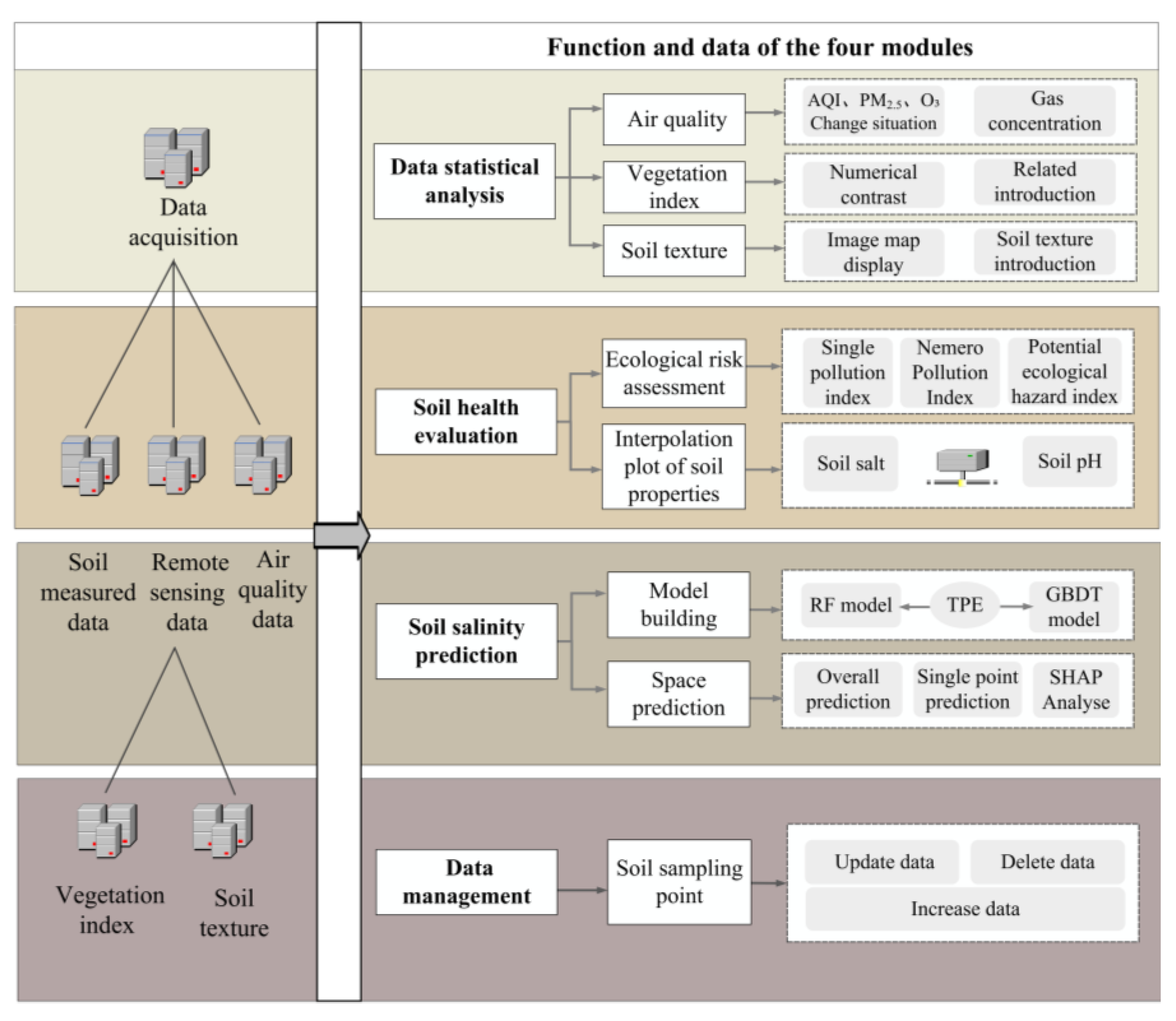
3. Design of WebGIS System Functions

The WebGIS system functions are hierarchically released to the server of the cloud platform according to the data response to support multi-level management and services of soil ecology and attribute prediction in the study area. The logical view of the functional architecture is designed as a tree structure, and the leftmost of Figure 8 is graded according to each type of data, including soil-measured data, remote sensing data, air quality data, vegetation index data, and soil texture data. On the right side of Figure 8, the functions are fully deployed, including data statistical analysis, soil health evaluation, soil salinity prediction, and data management. Moreover, the lowest level of leaves contains detailed functions and can be modularly expanded in the future based on new requirements.

3.1. Data Statistical Analysis

As the basis of the WebGIS system, this function displays and analyzes all spatial and non-spatial statistical data associated with the soil ecology of the study area, including air quality, vegetation index, and soil texture modules.

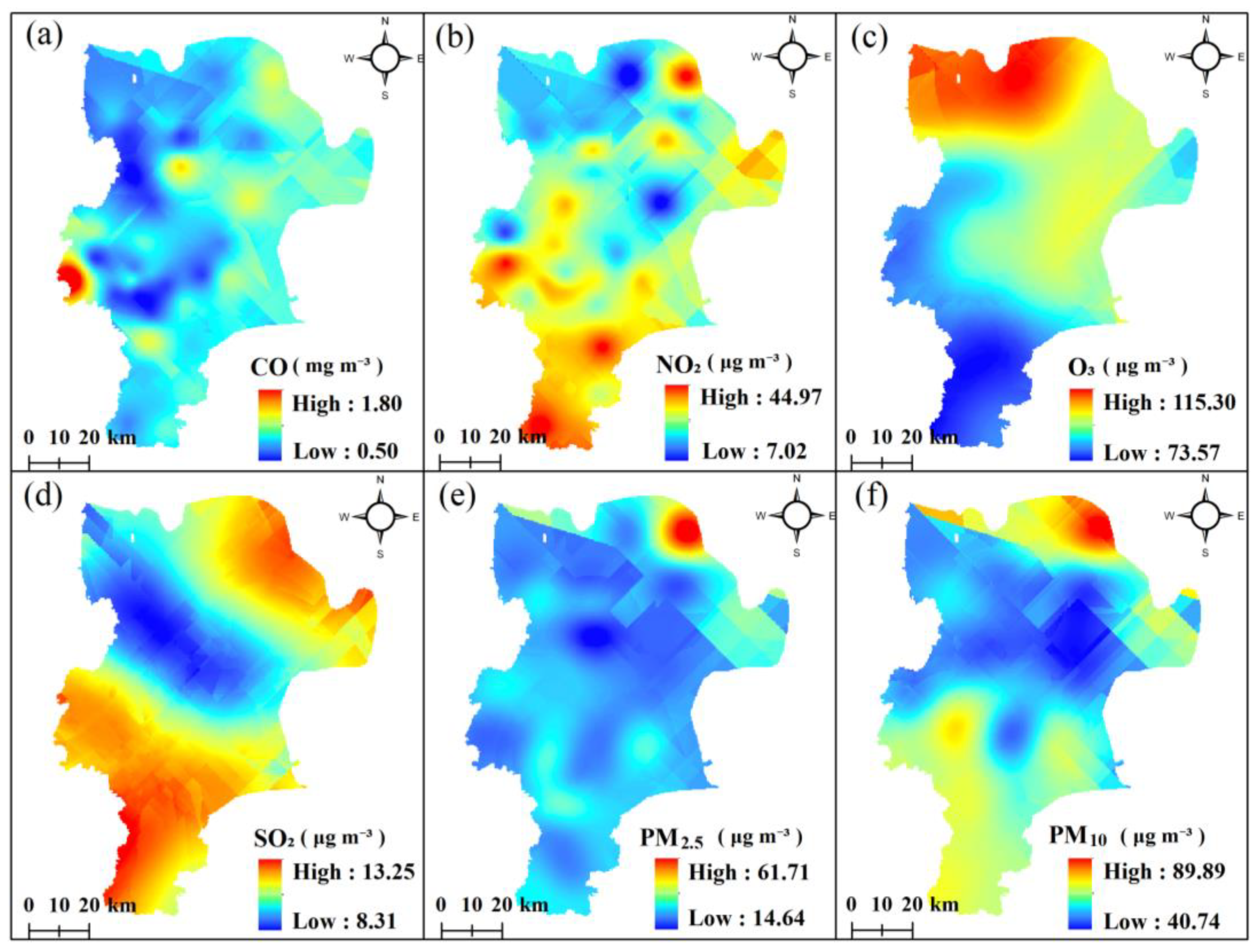
3.1.1. Air Quality Monitoring

In order to determine the air quality in the study area from multiple angles, a variety of display modes were used. These are statistical tables, statistical charts, and online maps. The statistical table (top left of Figure 9) shows the concentration standards of PM_2.5, O₃, PM₁₀, SO₂, NO_2, and CO, and the horizontal histogram (bottom left of Figure 9) shows the proportion of pollution gases in the primary and secondary standards. The longitudinal histogram reflects the monthly mean comparison results of the AQI index, which is high in winter and low in summer. At the far right of Figure 9, the user can select the monitoring station on the map to see the air quality pollution level of the current site. The pie chart shows the proportion of monthly concentrations of air quality such as O₃ and PM_2.5 in the total annual concentration.

In the main interface (in the middle of Figure 9), the user visually observes the spatial distribution of the polluting gases in the study area by selecting the interpolation map. This interpolation map is realized by using ArcGIS Server in the cloud server to publish the map. For example, by clicking the layer drop-down box to select SO₂ gas, the legend in the interface shows that the concentration of SO₂ is from 8.31 ug m⁻³ to 13.25 ug m⁻³. The SO₂ concentration in the northeast and south of the study area is higher, while the SO₂ concentration in the middle is lower. This function can help users identify the areas with serious air quality pollution, and take targeted measures to control the corresponding areas, which is conducive to timely control of air pollution.

3.1.2. Vegetation Index Analysis

Since the vegetation index is a relatively abstract concept for ordinary users, this function module provides the text of the introduction of the concept of vegetation index and the bubble diagram of its related applications (left side of Figure 10). Based on the above introduction, the user can easily understand the comparison results of descriptive statistics values from the vegetation index in the line chart. Through the map coverage analysis, the spatial distribution characteristics of the vegetation index in the study area and the proportion of the hierarchical area in the pie chart are clarified.

For example, by viewing the spatial interpolation results of the MNDVI index (Figure 10), users can intuitively analyze the sparse (green area) and dense (red area) distribution trends of the MNDVI index in the study area according to the color. The areas with higher MNDVI index values are concentrated near the seaside, and the vegetation coverage on both sides of the river in the inland area is higher, which may be associated with the dense number of nearby farmland, sufficient soil nutrients, and water content. In contrast, the MNDVI index is lower in the north and east. In this module, users can qualitatively infer the soil ecological situation of saline–alkali land in the study area by understanding the coverage characteristics of the vegetation.

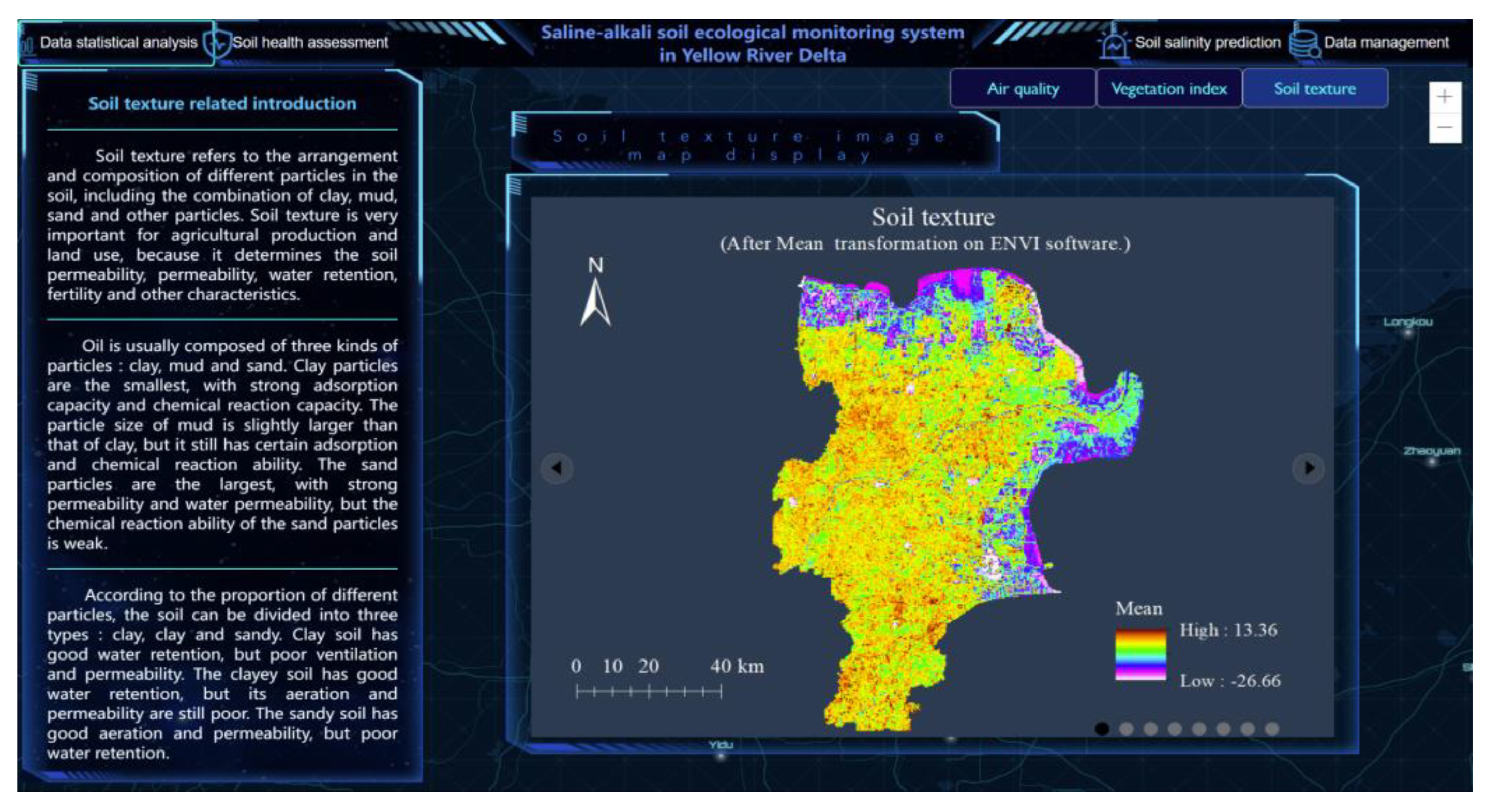
3.1.3. Soil Texture Analysis

In order to allow users to understand the soil texture characteristics in the study area, the concepts of soil texture, particle composition, and texture type are provided on the left side of Figure 11. In the main interface, the remote sensing images of eight soil textures in the study area are displayed, including Mean, VAR, HOM, CTRA, DIS, ENT, SECM, and CORR, and users can browse them by switching the arrow buttons around. For example, users can clearly observe the characteristics of soil texture with color change after Mean transformation in the region. The soil textures (purple and blue patches) near the ocean are homogeneous because the land use types (mainly wetlands and tidal flats) in these areas are monotonous. The yellow, green, and brown patches far from the ocean have high texture features. In these areas, farmland, forest land, grassland, construction land, and other land use types are mixed, resulting in complex soil texture features. This functional module can provide data support for assisting with farmland soil ecological assessment and spatial prediction of soil properties.

3.2. Soil Health Assessment

3.2.1. Ecological Risk Assessment

The ecological risk assessment function includes the single pollution index, Nemero comprehensive pollution index, and Hakanson potential ecological hazard index. Users can browse the rating criteria for each pollution index by clicking on the tab ‘See the evaluation criteria’. Taking Hakanson ecological risk assessment as an example (Figure 12), first, a single sampling point was selected to obtain id, latitude, and longitude information, and then the concentrations of As, Pb, and Zn in the soil were determined as 25.377 mg kg⁻¹, 27.383 mg kg⁻¹, and 38.163 mg kg⁻¹ by clicking on the tab ‘View the data for that point’. Finally, the Hakanson potential ecological risk index of this point was calculated. At the bottom of Figure 12, the comprehensive index, RI, is 35.913, indicating that this point is at a minor ecological risk level. The bar chart shows that although the concentrations of the three heavy metals were at a low ecological risk level, the Hakanson potential ecological risk index value of As in the soil was significantly higher than those of Pb and Zn, indicating that As had higher accumulation and ecological risk. Similarly, users can also choose the single pollution index and the Nemero comprehensive pollution index to evaluate soil ecology to determine whether the soil in the area is polluted with heavy metals.

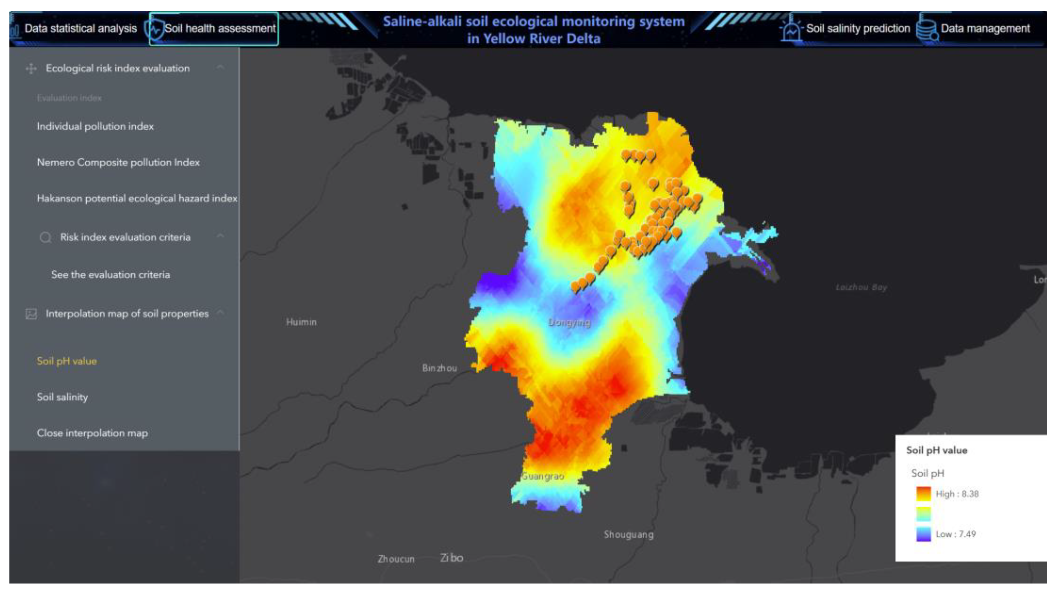
3.2.2. Evaluation of Spatial Variability of Soil Properties

Users can select the spatial distribution results of different soil properties in the left column, which can intuitively show the spatial variability of soil pH and soil salinity in the region. For example, the areas with high soil pH values were concentrated in the north and south of the study area (Figure 13), indicating that soil alkalinity in these areas was strong and the distribution had significant spatial heterogeneity. Users can prevent and control salinization according to the spatial variability of soil pH and salinity, and improve crop yield and quality by improving soil quality.

3.3. Spatial Prediction of Soil Salinity

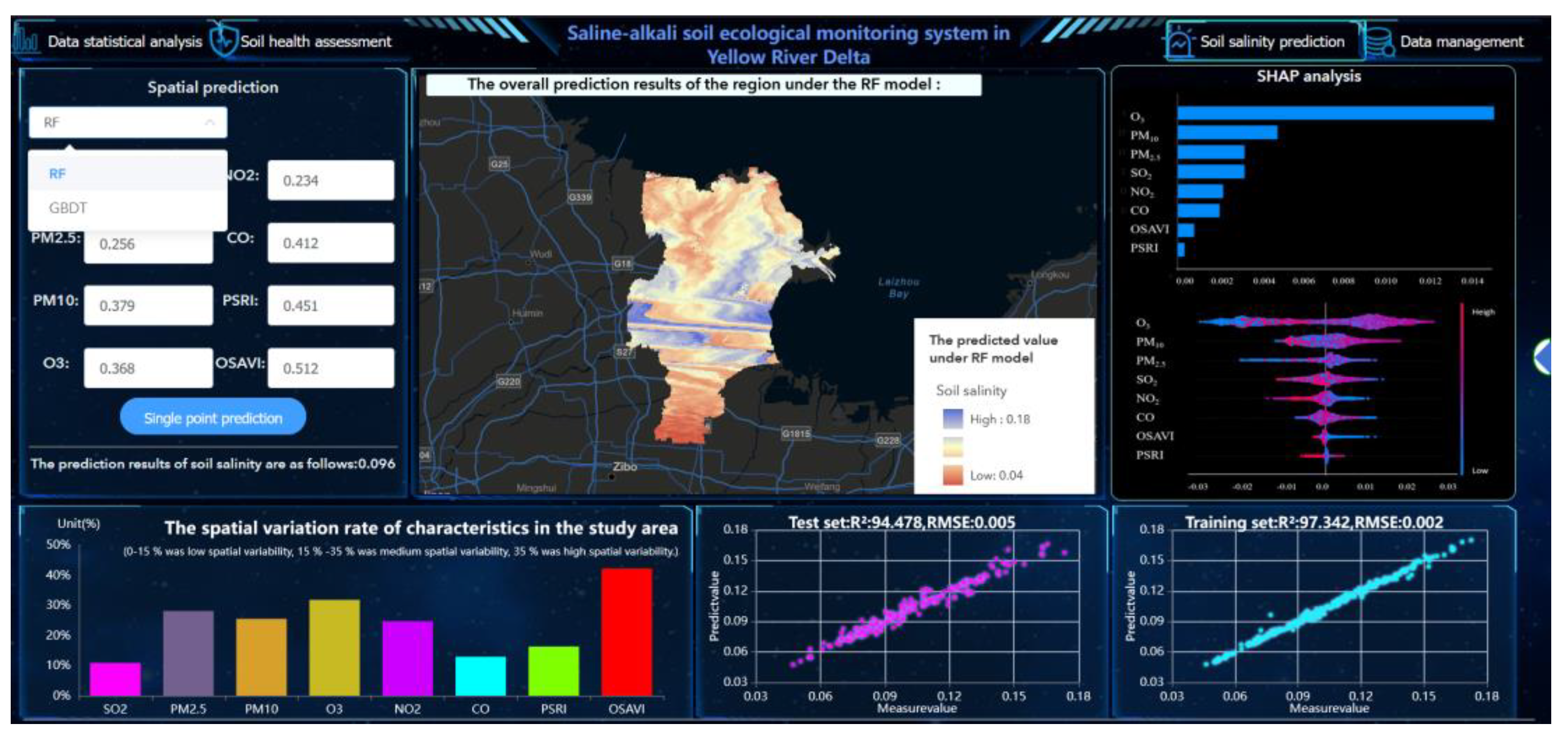
3.3.1. TPE–ML Prediction

Figure 14 shows the soil salinity prediction function module, which uses TPE–RF and TPE–GBDT models to predict soil salinity. The interface shows the prediction accuracy, spatial prediction map, scatter plot of the test set and training set, and SHAP analysis results. The module has a text box for user-defined prediction. By inputting the values of multiple feature indicators, the TPE-optimized machine learning model is called at the back end to perform single-point prediction of soil salinity. For example, the upper left of Figure 14 shows that the predicted single-point salinity based on the TPE–RF model is 0.096 g kg⁻¹. Compared with the TPE–GBDT model, the fitting accuracy of the TPE–RF model in the test set (R² = 94.48%) was higher, indicating that the TPE–RF model has a strong ability to explain the nonlinear relationship between environmental variables and soil salinity. The scatter plots of the training set and the test set of the TPE–RF model show better compactness along the diagonal.

3.3.2. SHAP-Based Variable Importance Analysis

The SHAP analysis results (upper right of Figure 14) show the total importance of different environmental variables in the prediction process (i.e., histogram). The higher the SHAP value, the greater the contribution of this factor to the fitting accuracy of soil salinity. The positive and negative driving effects and the cumulative importance of environmental variables at each point are also shown in the scatter plot of Figure 14. When the red points are gathered in the positive area on the right side of the coordinate axis and the blue points are gathered in the negative area on the left side of the coordinate axis, it means that the factor has a positive driving effect on soil salinity, and vice versa. For example, air quality factors (O₃ and PM₁₀) have a significant positive driving effect on the fitting accuracy of soil salinity, while SO₂ and NO₂ have a negative driving effect on the fitting accuracy of soil salinity. In addition, the coefficient of variation was used to describe the variation degree of soil salinity and various characteristics in the lower left of the system. If the variation rate of a feature is high, it means that the data is discrete and has high variability.

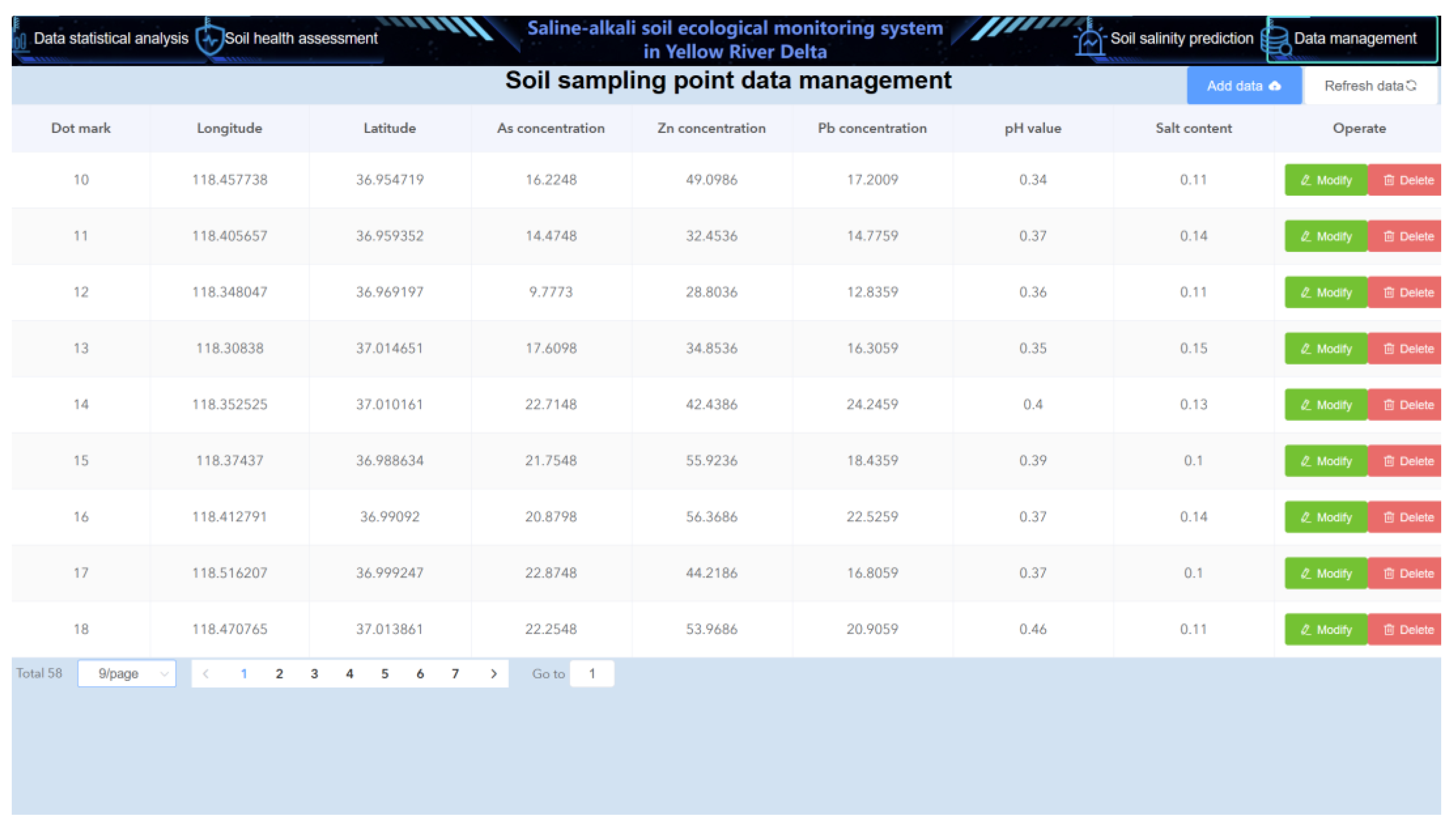
3.4. Data Management

The data management module shows detailed information on soil sampling points (Figure 15), which allows users to quickly browse, query, and operate the data. The main interface of the data module includes options to add data, modify data, delete data, and refresh data, as well as other functions. The user can click on the add data and enter the index information for the soil sampling point to add the sampling point data. The user can also click the modify button to modify the data for the sampling point according to the dynamic change in sampling point information to help the user update the data information in time. This module can realize comprehensive management of soil sampling point data.

4. Discussion

4.1. The Application Prospect of Hyperparameter Optimization Machine Learning in the WebGIS System

Prediction of soil properties is essential for monitoring soil ecological health, and the selection of accurate models and algorithms is the key to soil attribute prediction. The application of accurate algorithms or models in the WebGIS system can improve the accuracy of prediction and achieve more desirable results, which is consistent with the development trends for the existing WebGIS system. For example, Sciortino et al. applied the SL algorithm to WebGIS and used the SL prediction model to monitor the change in product shelf life, which enabled real-time prediction of shelf life [60]. Yong et al. applied an exponential smoothing prediction model in the WebGIS system to predict heavy metal pollution in the soil [15]. The results showed that the exponential smoothing prediction model could predict heavy metal soil pollution well. With the development of automatic machine learning algorithms, hyperparameter optimization is a key step to improving the prediction accuracy and generalization ability of machine learning models [61]. This system applied the TPE algorithm to optimize the key hyperparameters of RF and GBDT models, which significantly improved the prediction accuracy of the models.

The traditional hyperparameter optimization method of manual parameter adjustment or grid search has uncertainty and can easily fall into the local optimal solution, which has a high search time cost and poor performance. The TPE algorithm has been proven to be a high-performance parameter-tuning method in many studies [62,63]. It will select the next soil sampling point based on the performance of the previous soil sampling point. In the process of conducting thousands of iterations, TPE will continue to approach the lowest value of the loss function and then find the optimal hyperparameters of the model with a low time cost. The advantage of applying the TPE algorithm in this study is that it saves the time cost of hyperparameter optimization and significantly improves the prediction efficiency and fitting accuracy of the model. Combining WebGIS technology with TPE–RF and TPE–GBDT models achieves strong generalization ability and high-precision soil salinity prediction. However, in order to meet the needs of the WebGIS system to process massive multi-source heterogeneous data, embedding deep learning algorithms will be an inevitable trend to achieve high-precision prediction and processing of multi-dimensional data. Deep learning has a large number of hyperparameters and complex combinations, as well as stronger learning ability and generalization ability [64]. It also has immeasurable potential in dealing with multidimensional data of cross-scale fusion [65]. However, there are some difficulties at present. For example, unlike the decision tree model, the hyperparameter optimization interface of the neural network model needs to be clear. In particular, some deep neural networks such as CNN have complex hyperparameters and their hyperparameter optimization is very difficult. Future research should consider using the TPE algorithm to optimize the hyperparameters of the deep learning model to fully improve the computational efficiency of the system.

4.2. The Synergy of Multi-Source Environmental Variables in the WebGIS System

Considering that the use of multiple covariates can improve the prediction accuracy of the model, there is a large correlation between environmental variables that affect each other. In order to comprehensively monitor the ecological environment of the YRD, the system integrates multiple data sources associated with the soil ecological environment of the YRD in the data analysis layer, including air quality factor data, soil texture, vegetation index, soil attribute data, and other data. Using WebGIS technology, multi-source data sharing is realized in a visual form, helping users to comprehensively analyze and comprehensively monitor soil ecological health in the YRD. This is similar to the method of comprehensive analysis using multi-source data in the existing literature. Recently, Mallinis et al. used WebGIS technology to build a visual platform that integrates thematic data of all available ecosystem types, ecosystem ranges, ecosystem conditions, ecosystem services, and other information to help decision-makers conduct an overall assessment and comprehensive analysis of ecosystems [66]. Similarly, Yao et al. demonstrated a variety of data, including locust spatial data, field survey data, control data, and meteorological data, in the locust decision support system that are helpful for users to fully understand the occurrence of locust disasters and make decisions [18].

However, some limitations should also be taken into account. The integrity and availability of real-time data may be insufficient, which affects the accurate monitoring of the soil ecological environment. For example, the soil attribute data used in this system is obtained via manual field sampling. Due to the limitations of environment, resources, and technology, the sampling scale and sampling number are small, the spatial representation is poor, and the data integrity is insufficient, hence it is difficult to obtain data in real-time. Soil quality changes dynamically. Accurate monitoring of soil ecological environment over a wide range requires more complete data to provide support. For example, detailed field data such as drainage measures and soil microbes in saline–alkali land are important for evaluating soil ecological processes in saline–alkali land at the field scale and for developing specific field management and soil improvement programs [67]. It also requires real-time data updates. In this case, how to obtain more complete and real-time data is a key issue that needs to be solved. With the development of information technology, sensor technology continues to progress, and comprehensive and accurate soil data can be obtained. Google Earth Engine (GEE) is a publicly accessible platform that provides a large number of earth observation datasets for analysis worldwide, including satellite image data and real-time observation data from multiple sensors [68]. Future research can obtain soil parameters and other environmental variable factors through the GEE platform, and establish a complete YRD soil ecological database to better monitor the soil ecological environment accurately and in real time.

The system provides a visual platform for the monitoring of soil ecological environment. In the current policy, the use of soil ecological monitoring systems is essential for environmental monitoring and saline–alkali protection. At present, our system is applied to the local scale of the YRD region, which has good performance and high prediction accuracy and plays an important role in the monitoring of the soil ecological environment. Our country is rich in soil resources. In the future, we can consider applying the system to a wider range of areas. However, there may be differences in soil quality and soil properties in different regions, and the function of the system may be different in different regions. It is necessary for future research to introduce more environmental variable factors and build a rich and complete database. Some module functions should be added to the WebGIS system in future research. More vegetation indices should be explored to respond to soil ecological monitoring functions. In particular, a long-term series of vegetation indices should be added to the WebGIS system to realize the spatial and temporal dynamic monitoring of saline–alkali soil, including soil ecological degradation and erosion warning, soil ecological water holding capacity, and carbon sequestration capacity evaluation functions. In addition, the system is oriented to a wide range of groups. Considering that non-professional farmers may lack experience and knowledge, we provide the introduction and share relevant knowledge on various types of data in the system. Users can gain professional knowledge in the process of using the system. However, in order to improve the ease of use and stability of the system, the future WebGIS system should also be tested and improved for different groups of users.

5. Conclusions

This study developed a WebGIS-based system for saline–alkali soil ecological real-time monitoring. The system integrates a variety of WebGIS technologies. The front end of the system uses technologies such as Vue.js, Element UI, Axios, and Echarts.js to provide users with an intuitive and easy-to-use interactive interface. The back end uses the spring boot framework to improve the stability of the system input data. PMML and JPMML are used for cross-platform deployment of machine learning models so that the prediction model can be shared. Different from previous studies, this study takes into account the multi-source environmental variables and reflects the diversity of the soil ecosystem in the saline–alkali land in YRD. Users can comprehensively analyze and monitor the soil ecological environment through the system. The data statistical analysis module showed the monitoring results of air quality, vegetation index, and soil texture in a visual form. The soil health assessment module provided users with the risk assessment of heavy metals in the soil and the spatial variability of soil properties. The soil salinity prediction module introduces the advanced TPE algorithm to optimize the RF and GBDT models, which significantly improves the prediction accuracy. The data management module applies Mybatis-Plus technology, and users can update data in real time. This study realized a potential platform for users to monitor the soil ecological environment, which provides scientific decision support for salt reduction and carbon sequestration in saline–alkali land.

The link to the saline–alkali soil ecological monitoring system in the YRD http://101.200.195.72:88/2023ESRI/ (accessed on 8 April 2024). (The account number is administrator and the password is 123456).

References

1. Nizzetto, L.; Futter, M.; Langaas, S. Are Agricultural Soils Dumps for Microplastics of Urban Origin? Environ. Sci. Technol. 2016, 50, 10777–10779. [Google Scholar] [CrossRef] [PubMed]
2. Tilman, D.; Balzer, C.; Hill, J.; Befort, B.L. Global food demand and the sustainable intensification of agriculture. Proc. Natl. Acad. Sci. USA 2011, 108, 20260–20264. [Google Scholar] [CrossRef]
3. Lehmann, J.; Bossio, D.A.; Kogel-Knabner, I.; Rillig, M.C. The concept and future prospects of soil health. Nat. Rev. Earth Environ. 2020, 1, 544–553. [Google Scholar] [CrossRef] [PubMed]
4. Kong, X. China must protect high-quality arable land. Nature 2014, 506, 7. [Google Scholar] [CrossRef] [PubMed]
5. Sun, X.D.; Yuan, X.Z.; Jia, Y.; Feng, L.J.; Zhu, F.P.; Dong, S.S.; Liu, J.; Kong, X.; Tian, H.; Duan, J.L.; et al. Differentially charged nanoplastics demonstrate distinct accumulation in Arabidopsis thaliana. Nat. Nanotechnol. 2020, 15, 755–760. [Google Scholar] [CrossRef]
6. Hou, P.; Jiang, Y.; Yan, L.; Petropoulos, E.; Wang, J.; Xue, L.; Yang, L.; Chen, D. Effect of fertilization on nitrogen losses through surface runoffs in Chinese farmlands: A meta-analysis. Sci. Total Environ. 2021, 793, 148554. [Google Scholar] [CrossRef]
7. Chen, Z.; Huang, G.; Li, Y.; Zhang, X.; Xiong, Y.; Huang, Q.; Jin, S. Effects of the lignite bioorganic fertilizer on greenhouse gas emissions and pathways of nitrogen and carbon cycling in saline-sodic farmlands at Northwest China. J. Clean. Prod. 2022, 334, 130080. [Google Scholar] [CrossRef]
8. Wang, S.; Cai, L.M.; Wen, H.H.; Luo, J.; Wang, Q.S.; Liu, X. Spatial distribution and source apportionment of heavy metals in soil from a typical county-level city of Guangdong Province, China. Sci. Total Environ. 2019, 655, 92–101. [Google Scholar] [CrossRef]
9. Tchounwou, P.B.; Yedjou, C.G.; Patlolla, A.K.; Sutton, D.J. Heavy metal toxicity and the environment. Exp. Suppl. 2012, 101, 133–164. [Google Scholar]
10. Yang, Z.; Shi, W.; Yang, W.; Liang, L.; Yao, W.; Chai, L.; Gao, S.; Liao, Q. Combination of bioleaching by gross bacterial biosurfactants and flocculation: A potential remediation for the heavy metal contaminated soils. Chemosphere 2018, 206, 83–91. [Google Scholar] [CrossRef]
11. de Paul Obade, V.; Lal, R. Assessing land cover and soil quality by remote sensing and geographical information systems (GIS). Catena 2013, 104, 77–92. [Google Scholar] [CrossRef]
12. Xia, X.; Yang, Z.; Yu, T.; Hou, Q.; Mutelo, A.M. Detecting changes of soil environmental parameters by statistics and GIS: A case from the lower Changjiang plain, China. J. Geochem. Explor. 2017, 181, 116–128. [Google Scholar] [CrossRef]
13. Kourgialas, N.N.; Hliaoutakis, A.; Argyriou, A.V.; Morianou, G.; Voulgarakis, A.E.; Kokinou, E.; Daliakopoulos, I.N.; Kalderis, D.; Tzerakis, K.; Psarras, G.; et al. A web-based GIS platform supporting innovative irrigation management techniques at farm-scale for the Mediterranean island of Crete. Sci. Total Environ. 2022, 842, 156918. [Google Scholar] [CrossRef] [PubMed]
14. Mourato, S.; Fernandez, P.; Marques, F.; Rocha, A.; Pereira, L. An interactive Web-GIS fluvial flood forecast and alert system in operation in Portugal. Int. J. Disast. Risk Re. 2021, 58, 102201. [Google Scholar] [CrossRef]
15. Yong, M.; Zhang, M.; Wang, S.; Liu, G. A Flex and ArcGIS Server based system for farmland environmental quality assessment and prediction in an agricultural producing area. Comput. Electron. Agric. 2015, 112, 193–199. [Google Scholar] [CrossRef]
16. McCord, P.; Tonini, F.; Liu, J. The Telecoupling GeoApp: A Web-GIS application to systematically analyze telecouplings and sustainable development. Appl. Geogr. 2018, 96, 16–28. [Google Scholar] [CrossRef]
17. Kawasaki, A.; Berman, M.L.; Guan, W. The growing role of web-based geospatial technology in disaster response and support. Disasters 2013, 37, 201–221. [Google Scholar] [CrossRef]
18. Yao, X.; Zhu, D.; Yun, W.; Peng, F.; Li, L. A WebGIS-based decision support system for locust prevention and control in China. Comput. Electron. Agric. 2017, 140, 148–158. [Google Scholar] [CrossRef]
19. Feng, Q.; Flanagan, D.C.; Engel, B.A.; Yang, L.; Chen, L. GeoAPEXOL, a web GIS interface for the Agricultural Policy Environmental eXtender (APEX) model enabling both field and small watershed simulation. Environ. Modell. Softw. 2020, 123, 104569. [Google Scholar] [CrossRef]
20. Cao, Q.; Yang, L.; Ren, W.; Song, Y.; Huang, S.; Wang, Y.; Wang, Z. Spatial distribution of harmful trace elements in Chinese coalfields: An application of WebGIS technology. Sci. Total Environ. 2021, 755, 142527. [Google Scholar] [CrossRef]
21. Alvioli, M.; Falcone, G.; Mendicelli, A.; Mori, F.; Fiorucci, F.; Ardizzone, F.; Moscatelli, M. Seismically induced rockfall hazard from a physically based model and ground motion scenarios in Italy. Geomorphology 2023, 429, 108652. [Google Scholar] [CrossRef]
22. Biolchi, L.G.; Unguendoli, S.; Bressan, L.; Giambastiani, B.M.S.; Valentini, A. Ensemble technique application to an XBeach-based coastal Early Warning System for the Northwest Adriatic Sea (Emilia-Romagna region, Italy). Coast. Eng. 2022, 173, 104081. [Google Scholar] [CrossRef]
23. Jia, Y.; Zhao, H.; Niu, C.; Jiang, Y.; Gan, H.; Xing, Z.; Zhao, X.; Zhao, Z. A WebGIS-based system for rainfall-runoff prediction and real-time water resources assessment for Beijing. Comput. Geosci. 2009, 35, 1517–1528. [Google Scholar] [CrossRef]
24. Thiebes, B.; Bell, R.; Glade, T.; Jäger, S.; Anderson, M.; Holcombe, L. A WebGIS decision-support system for slope stability based on limit-equilibrium modelling. Eng. Geol. 2013, 158, 109–118. [Google Scholar] [CrossRef]
25. Zuan, C.; Jingyu, B. The Design of Typhoon Meteorological Information System and its Implementation Based on WebGIS. Procedia Environ. Sci. 2011, 10, 420–426. [Google Scholar] [CrossRef]
26. Habibi, V.; Ahmadi, H.; Jafari, M.; Moeini, A. Machine learning and multispectral data-based detection of soil salinity in an arid region, Central Iran. Environ. Monit. Assess. 2020, 192, 759. [Google Scholar] [CrossRef] [PubMed]
27. Xiao, C.; Ji, Q.; Chen, J.; Zhang, F.; Li, Y.; Fan, J.; Hou, X.; Yan, F.; Wang, H. Prediction of soil salinity parameters using machine learning models in an arid region of northwest China. Comput. Electron. Agric. 2023, 204, 107512. [Google Scholar] [CrossRef]
28. Azizi, K.; Ayoubi, S.; Nabiollahi, K.; Garosi, Y.; Gislum, R. Predicting heavy metal contents by applying machine learning approaches and environmental covariates in west of Iran. J. Geochem. Explor. 2022, 233, 106921. [Google Scholar] [CrossRef]
29. Liu, G.; Tian, S.; Xu, G.; Zhang, C.; Cai, M. Combination of effective color information and machine learning for rapid prediction of soil water content. J. Rock Mech. Geotech. 2023, 15, 2441–2457. [Google Scholar] [CrossRef]
30. Hutter, F.; Kotthoff, L.; Vanschoren, J. Automated Machine Learning: Methods, Systems, Challenges; Springer Nature: New York, NY, USA, 2019. [Google Scholar]
31. Chen, B.; Zheng, H.; Luo, G.; Chen, C.; Bao, A.; Liu, T.; Chen, X. Adaptive estimation of multi-regional soil salinization using extreme gradient boosting with Bayesian TPE optimization. Int. J. Remote Sens. 2022, 43, 778–811. [Google Scholar] [CrossRef]
32. Yan, H.; Yan, K.; Ji, G. Optimization and prediction in the early design stage of office buildings using genetic and XGBoost algorithms. Build. Environ. 2022, 218, 109081. [Google Scholar] [CrossRef]
33. Song, Y.; Zhan, D.; He, Z.; Li, W.; Duan, W.; Yang, Z.; Lu, M. HPO-empowered machine learning with multiple environment variables enables spatial prediction of soil heavy metals in coastal delta farmland of China. Comput. Electron. Agric. 2023, 213, 108254. [Google Scholar] [CrossRef]
34. Rodriguez-Galiano, V.; Sanchez-Castillo, M.; Chica-Olmo, M.; Chica-Rivas, M. Machine learning predictive models for mineral prospectivity: An evaluation of neural networks, random forest, regression trees and support vector machines. Ore Geol. Rev. 2015, 71, 804–818. [Google Scholar] [CrossRef]
35. Zhang, W.; Zhang, R.; Wu, C.; Goh, A.T.C.; Lacasse, S.; Liu, Z.; Liu, H. State-ofthe-art review of soft computing applications in underground excavations. Geosci. Front. 2020, 11, 1095–1106. [Google Scholar] [CrossRef]
36. Feng, Y.; Wang, D.; Yin, Y.; Li, Z.; Hu, Z. An XGBoost-based casualty prediction method for terrorist attacks. Complex Intell. Syst. 2020, 6, 721–740. [Google Scholar] [CrossRef]
37. Zhan, D.; Mu, Y.; Duan, W.; Ye, M.; Song, Y.; Song, Z.; Yao, K.; Sun, D.; Ding, Z. Spatial Prediction and Mapping of Soil Water Content by TPE-GBDT Model in Chinese Coastal Delta Farmland with Sentinel-2 Remote Sensing Data. Agriculture 2023, 13, 1088. [Google Scholar] [CrossRef]
38. Yu, J.; Zheng, W.; Xu, L.; Meng, F.; Li, J.; Zhangzhong, L. TPE-CatBoost: An adaptive model for soil moisture spatial estimation in the main maize-producing areas of China with multiple environment covariates. J. Hydrol. 2022, 613, 128465. [Google Scholar] [CrossRef]
39. Chen, C.; Seo, H. Prediction of rock mass class ahead of TBM excavation face by ML and DL algorithms with Bayesian TPE optimization and SHAP feature analysis. Acta Geotech. 2023, 18, 3825–3848. [Google Scholar] [CrossRef]
40. Frampton, W.J.; Dash, J.; Watmough, G.; Milton, E.J. Evaluating the capabilities of Sentinel-2 for quantitative estimation of biophysical variables in vegetation. ISPRS J. Photogramm. 2013, 82, 83–92. [Google Scholar] [CrossRef]
41. Liu, Q.; Yao, F.; Garcia-Garcia, A.; Zhang, J.; Li, J.; Ma, S.; Li, S.; Peng, J. The response and sensitivity of global vegetation to water stress: A comparison of different satellite-based NDVI products. Int. J. Appl. Earth Obs. 2023, 120, 103341. [Google Scholar] [CrossRef]
42. Rondeaux, G.; Steven, M.; Baret, F. Optimization of soil-adjusted vegetation indices. Remote Sens. Environ. 1996, 55, 95–107. [Google Scholar] [CrossRef]
43. Fernández-Manso, A.; Fernández-Manso, O.; Quintano, C. SENTINEL-2A red-edge spectral indices suitability for discriminating burn severity. Int. J. Appl. Earth Obs. 2016, 50, 170–175. [Google Scholar] [CrossRef]
44. Lam, E.J.; Urrutia, J.; Bech, J.; Herrera, C.; Montofre, I.L.; Zetola, V.; Alvarez, F.A.; Canovas, M. Heavy metal pollution index calculation in geochemistry assessment: A case study on Playa Las Petroleras. Environ. Geochem. Health 2023, 45, 409–426. [Google Scholar] [CrossRef]
45. Tang, M.; Hou, J. Statistical Analysis and Evaluation of Heavy Metal Ions in Soil Environment. Open Access Libr. J. 2016, 03, 1–8. [Google Scholar] [CrossRef]
46. Yan, F.; Li, N.; Wang, J.; Wu, H. Ecological footprint model of heavy metal pollution in water environment based on the potential ecological risk index. J. Environ. Manag. 2023, 344, 118708. [Google Scholar] [CrossRef] [PubMed]
47. Sá, D.; Guimarães, T.; Abelha, A.; Santos, M.F. Low Code Approach for Business Analytics. Procedia Compu. Sci. 2024, 231, 421–426. [Google Scholar] [CrossRef]
48. Li, D.; Mei, H.; Shen, Y.; Su, S.; Zhang, W.; Wang, J.; Zu, M.; Chen, W. ECharts: A declarative framework for rapid construction of web-based visualization. Visual Inform. 2018, 2, 136–146. [Google Scholar] [CrossRef]
49. Suryotrisongko, H.; Jayanto, D.P.; Tjahyanto, A. Design and Development of Backend Application for Public Complaint Systems Using Microservice Spring Boot. Procedia Comput. Sci. 2017, 124, 736–743. [Google Scholar] [CrossRef]
50. Li, Y.; Gao, S.; Pan, J.; Guo, B.F.; Xie, P.F. Research and Application of Template Engine for Web Back-end Based on MyBatis-Plus. Procedia Comput. Sci. 2020, 166, 206–212. [Google Scholar] [CrossRef]
51. Jiang, B.N.; Zhang, Y.Y.; Zhang, Z.Y.; Yang, Y.L.; Song, H.L. Tree-structured parzen estimator optimized-automated machine learning assisted by meta-analysis for predicting biochar-driven N(2)O mitigation effect in constructed wetlands. J. Environ. Manag. 2024, 354, 120335. [Google Scholar] [CrossRef]
52. Jiang, F.; Kutia, M.; Sarkissian, A.J.; Lin, H.; Long, J.; Sun, H.; Wang, G. Estimating the Growing Stem Volume of Coniferous Plantations Based on Random Forest Using an Optimized Variable Selection Method. Sensors 2020, 20, 7248. [Google Scholar] [CrossRef] [PubMed]
53. Cutler, D.R.; Edwards, T.J.; Beard, K.H.; Cutler, A.; Hess, K.T.; Gibson, J.; Lawler, J.J. Random forests for classification in ecology. Ecology 2007, 88, 2783–2792. [Google Scholar] [CrossRef] [PubMed]
54. Zhang, W.; Yu, J.; Zhao, A.; Zhou, X. Predictive model of cooling load for ice storage air-conditioning system by using GBDT. Energy Rep. 2021, 7, 1588–1597. [Google Scholar] [CrossRef]
55. Yu, Z.; Wang, Z.; Zeng, F.; Song, P.; Baffour, B.A.; Wang, P.; Wang, W.; Li, L. Volcanic lithology identification based on parameter-optimized GBDT algorithm: A case study in the Jilin Oilfield, Songliao Basin, NE China. J. Appl. Geophys. 2021, 194, 104443. [Google Scholar] [CrossRef]
56. Ren, X.; Mi, Z.; Cai, T.; Nolte, C.G.; Georgopoulos, P.G. Flexible Bayesian Ensemble Machine Learning Framework for Predicting Local Ozone Concentrations. Environ. Sci. Technol. 2022, 56, 3871–3883. [Google Scholar] [CrossRef] [PubMed]
57. Zhang, Y.; Li, L.; Ren, Z.; Yu, Y.; Li, Y.; Pan, J.; Lu, Y.; Feng, L.; Zhang, W.; Han, Y. Plant-scale biogas production prediction based on multiple hybrid machine learning technique. Bioresour. Technol. 2022, 363, 127899. [Google Scholar] [CrossRef] [PubMed]
58. Rahrooh, A.; Garlid, A.O.; Bartlett, K.; Coons, W.; Petousis, P.; Hsu, W.; Bui, A.A.T. Towards a framework for interoperability and reproducibility of predictive models. J. Biomed. Inform. 2024, 149, 104551. [Google Scholar] [CrossRef] [PubMed]
59. Shin, S.; Um, J. Integrating Predictive Model Markup Language with Asset Administration Shell. IFAC-Pap. 2023, 56, 9823–9830. [Google Scholar] [CrossRef]
60. Sciortino, R.; Micale, R.; Enea, M.; La Scalia, G. A webGIS-based system for real time shelf life prediction. Comput. Electron. Agric. 2016, 127, 451–459. [Google Scholar] [CrossRef]
61. Sraitih, M.; Jabrane, Y.; Hajjam, E.H.A. An Automated System for ECG Arrhythmia Detection Using Machine Learning Techniques. J. Clin. Med. 2021, 10, 5450. [Google Scholar] [CrossRef]
62. Nguyen, H.; Liu, J.; Zio, E. A long-term prediction approach based on long short-term memory neural networks with automatic parameter optimization by Tree-structured Parzen Estimator and applied to time-series data of NPP steam generators. Appl. Soft Comput. 2020, 89, 106116. [Google Scholar] [CrossRef]
63. Wang, S.; Gao, W.; Ming, J.; Li, L.; Xu, D.; Liu, S.; Lu, J. A TPE based inversion of PROSAIL for estimating canopy biophysical and biochemical variables of oilseed rape. Comput. Electron. Agric. 2018, 152, 350–362. [Google Scholar] [CrossRef]
64. Jiang, Y.; Li, C.; Song, H.; Wang, W. Deep learning model based on urban multi-source data for predicting heavy metals (Cu, Zn, Ni, Cr) in industrial sewer networks. J. Hazard. Mater. 2022, 432, 128732. [Google Scholar] [CrossRef]
65. Zheng, J.; Yuan, S.; Wu, W.; Li, W.; Yu, L.; Fu, H.; Coomes, D. Surveying coconut trees using high-resolution satellite imagery in remote atolls of the Pacific Ocean. Remote Sens. Environ. 2023, 287, 113485. [Google Scholar] [CrossRef]
66. Mallinis, G.; Chalkidou, S.; Roustanis, T.; Kokkoris, I.P.; Chrysafis, I.; Karolos, I.; Vagiona, D.; Kavvadia, A.; Dimopoulos, P.; Mitsopoulos, I. A national scale web mapping platform for mainstreaming ecosystem services in Greece. Ecol. Inform. 2023, 78, 102349. [Google Scholar] [CrossRef]
67. Heng, T.; He, X.; Yang, L.; Xu, X.; Feng, Y. Mechanism of Saline–Alkali land improvement using subsurface pipe and vertical well drainage measures and its response to agricultural soil ecosystem. Environ. Pollut. 2022, 293, 118583. [Google Scholar] [CrossRef]
68. Ghosh, S.; Kumar, D.; Kumari, R. Cloud-based large-scale data retrieval, mapping, and analysis for land monitoring applications with Google Earth Engine (GEE). Environ. Chall. 2022, 9, 100605. [Google Scholar] [CrossRef]
Figure 1. The location of (c) the study area in (b) Shandong province of (a) China.
Remotesensing 16 01948 g001
Figure 2. Eight soil texture feature statistics: (a) Mean, (b) VAR, (c) HOM, (d) CTRA, (e) DIS, (f) ENT, (g) SECM, and (h) CORR. Four vegetation indices: (i) MNDVI, (j) NDVI, (k) OSAVI, and (l) PSRI.
Remotesensing 16 01948 g002
Figure 3. Spatial interpolation results for (a) CO, (b) NO2, (c) O3, (d) SO2, (e) PM2.5, and (f) PM10.
Remotesensing 16 01948 g003
Figure 4. The interpolation results for (a) soil pH and (b) soil salinity.
Remotesensing 16 01948 g004
Figure 5. Numerical statistics of heavy metals in soil.
Remotesensing 16 01948 g005
Figure 6. The architecture of the saline–alkali soil ecological monitoring system in the YRD.
Remotesensing 16 01948 g006
Figure 7. The architecture of database design.
Remotesensing 16 01948 g007
Figure 8. Functions of the saline–alkali soil ecological monitoring system in the YRD.
Remotesensing 16 01948 g008
Figure 9. The main interface of the air quality module.
Remotesensing 16 01948 g009
Figure 10. The main interface of the vegetation index module.
Remotesensing 16 01948 g010
Figure 11. The main interface of the soil texture module.
Remotesensing 16 01948 g011
Figure 12. The ecological risk assessment results of heavy metals in the soil system.
Remotesensing 16 01948 g012
Figure 13. The spatial distribution of soil pH concentrations.
Remotesensing 16 01948 g013
Figure 14. Prediction of soil salinity using the TPE–RF model.
Remotesensing 16 01948 g014
Figure 15. The main interface of the data management module.
Remotesensing 16 01948 g015