Time Phase Selection and Accuracy Analysis for Predicting Winter Wheat Yield Based on Time Series Vegetation Index

Abstract

Winter wheat is one of the major cereal crops globally and one of the top three cereal crops in China. The precise forecasting of the yield of winter wheat holds significant importance in the realms of agricultural management and ensuring food security. The use of multi-temporal remote sensing data for crop yield prediction has gained increasing attention. Previous research primarily focused on utilizing remote sensing data from individual or a few growth stages as input parameters or integrated data across the entire growth period. However, a detailed analysis of the impact of different temporal combinations on the accuracy of yield prediction has not been extensively reported. In this study, we optimized the temporal sequence of growth stages using interpolation methods, constructed a yield prediction model incorporating the enhanced vegetation index (EVI) at different growth stages as input parameters, and employed a random forest (RF) algorithm. The results indicated that the RF model utilizing the EVI from all the temporal combinations throughout the growth period as input parameters accurately predicted the winter wheat yield with an R² of the calibrated dataset exceeding 0.58 and an RMSE less than 1284 kg/ha. Among the 1023 yield models tested in this study with ten different growth stage combinations, the most accurate temporal combination comprised five stages corresponding to the regreening, erecting, jointing, heading, and filling stages, with an R² of 0.81 and an RMSE of 1250 kg/ha and an NRMSE of 15%. We also observed a significant decrease in estimation accuracy when the number of growth stages was fewer than five and a certain degree of decline when the number exceeded five. Our findings confirmed the optimal number and combination of growth stages for the best yield prediction, providing substantial insights for winter wheat yield forecasting.

1. Introduction

Wheat is one of the world’s major cereal crops, accounting for approximately 40% of the global food supply, with an estimated 60% increase in demand projected by 2050 [1]. However, the current winter wheat production rates are expected to fall short of meeting the anticipated yields by 2050 [2]. China, as the world’s largest producer and consumer of wheat, contributes 18% to global wheat production [3]. The yield of winter wheat is not only influenced by the slowing growth trend, but also susceptible to various socio-economic factors (such as agricultural policies, labor, and management) and natural disasters (including extreme temperatures, pests, droughts, and floods) [4]. The timely and accurate prediction of winter wheat yield is crucial for crop management, food security, and sustainable agricultural development [5].

The traditional methods of obtaining the crop yield, such as field survey methods, involve on-site investigations and destructive sampling analysis, estimating the actual yields by sampling a portion of crop samples in the field [6]. The field survey method is also affected by reliability problems caused by response decline, resource limitation, sampling error, and spatial distribution, and it has disadvantages, such as a high cost and labor consumption [7]. In addition, the results of field investigations typically have to wait until the crop has been harvested, so the agricultural activities cannot be adjusted promptly and accurately according to the expected yield in the process of crop growth to cope with emergencies [8]. In recent years, the rapid development of satellite remote sensing technology has resulted in widespread attention on remote sensing methods for estimating yield. As an accurate, dynamic, macro, and rapid monitoring tool, satellite-based remote sensing technology relies on satellite images to capture the growth state of crops during their growth process, and then combines the estimation algorithm to achieve yield prediction [9]. Images from the Sentinel-2 satellite are being used more and more widely. Most of the Sentinel-2 image data are downloaded from Google Earth Engine (GEE, Google Inc., Mountain View, CA, USA) [8].

Remote sensing-based crop yield estimation models typically fall into categories such as light use efficiency (LUE) models, data assimilation (DA) models, and empirical statistical models (ESMs). Among them, the vegetation index is an important input parameter. Initially, the satellite-based LUE models were designed to evaluate the gross primary product of vegetation, and then to estimate the yield by converting the gross primary product into the proportion of crop organs harvested [10]. Although LUE models simplify the parameter inputs, they still face limitations in terms of cumulative errors and reusability [10]. DA models integrate remote sensing information into crop growth models, minimizing the differences between remote sensing observations and model variables [5] to better simulate the crop growth conditions, and thus obtain more accurate regional yield estimates. This model based on remote sensing data, and the crop growth model has a better mechanism interpretation, but it ignores the errors in the observed data and is affected by the difficulty in obtaining the parameters of the crop growth model, resulting in large uncertainties in the estimation of regional crop yield on a large scale [11]. ESMs predict yields by identifying the linear relationships between predicting variables in a given dataset and historical crop yields [12]. This model is simple to calculate and has strong explanatory power, which can be used for regional-scale uncertainty analysis. However, ESMs do not consider the growth process of crops. The collinearity problem between predictor variables or prior steady-state hypothesis is the main limitation when dealing with a series of large multi-variable datasets, and challenges arise in dealing with nonlinear relations between variables. At the same time, ESMs result in poor spatial generalization for large areas [6,13]. To solve these problems, machine learning algorithms that can capture complex nonlinear relationships and process high-dimensional data have been widely used.

Machine learning involves a learning process that aims to perform tasks based on “experience” (training data) [9]. Given that machine learning algorithms combine the advantages of other methods, such as statistical models and crop growth models, machine learning is becoming an indispensable tool in crop yield modeling and precision agriculture [14]. In the algorithm of machine learning, random forest (RF) is an important non-parametric advanced classification and regression tree analysis method among the integrated learning methods [15]. Jeong et al. used crop yield data for model training and testing and found that RF has a strong ability to predict crop yield. RF is a machine learning method with great potential in yield estimation [12]. RF has the advantages of high accuracy, data analysis practicability, and ease of use [16]. Han et al. used a variety of different parameter combinations as inputs to construct an RF model to predict yield and achieved great advantages in winter wheat yield prediction [17].

Crop growth is an allometric growth process, but most researchers ignore the fact that there are significant differences in crops at different growth stages. Some of these yield estimation models are limited to a single growth stage to make the prediction accuracy low, and some have the problem of an unstable performance across growth periods [18]. Therefore, a certain gap remains in the research of using remote sensing data to consider the impact of relative yield prediction at different growth stages. The rapid improvement in Earth observation has also made multi-temporal crop observation a feasible reality [19]. Researchers are no longer limited to a single date or a single growth stage for yield prediction [18,20], and they show that a yield prediction model matching the crop growth stage makes precision agriculture management more cost-effective and operable. Recently, Han et al. modeled and predicted winter wheat yield at the five key growth stages of winter wheat, demonstrating that the yield estimation model can show better results when considering multi-temporal sequence remote sensing information [17]. Wang et al. determined the optimal stage and spectral index for wheat yield and quality prediction using multi-temporal remote sensing data, and the estimation accuracy was high [21].

In the existing studies, there are some combinations of data acquired by different satellites that reduce the problem of missing images caused by weather. While multi-source satellite data can provide a comprehensive view at different scales, they also introduce challenges, such as increased computational complexity and the possible introduction of errors in the data fusion process [22,23]. The use of an interpolation method to simulate the missing data can optimize the time series data [24]. Fu et al. used a linear interpolation method to optimize the NDVI time series; the winter wheat yield was predicted with high accuracy. Based on the data measured at the site, Wu et al. used the interpolation method to obtain daily meteorological data and input them into the model for estimation [25]. Li et al. used five interpolation methods to interpolate vegetation index time series data (linear interpolation, a piecewise logistic function, a polynomial curve function, an asymmetric Gaussian function, and spline interpolation). It was found that these methods are effective to optimize the data [26].

Although these studies use growth stage remote sensing data as part of the prediction variables, they do not specify which growth stage or combination of growth stages of the crop contributes more to the improvement of the yield prediction accuracy. Based on these studies, this paper will carry out the following work: (1) During the complete growth cycle of winter wheat, the vegetation index with a stable and good correlation with yield was screened. (2) The optimal interpolation method was selected to optimize and smooth the time series data of the whole growth stage to substitute for the missing growth stage image data. (3) The RF model, the number, and the combination of time phases that can improve the accuracy of the winter wheat yield estimation model were evaluated.

2. Materials and Methods

2.1. Study Area

The study area is located in Shandong Province (Figure 1b), including two regions. The first study area (Figure 1c) is located in Mingji Town, Binzhou City, China (from 36.88°N to 36.98°N, from 117.53°E to 117.67°E, with an altitude of 4–36 m). The study area is located in a temperate monsoon region, with a temperate continental monsoon climate. The yearly mean duration of sunshine amounts to 2619.3 h, with an average annual temperature of 13.0 °C, coupled with an approximate annual precipitation of 690 mm. The second study area (Figure 1d) is located in the southwest of Pingdu City, Qingdao City, China (from 36.78°N to 36.81°N, from 119.72°E to 119.75°E, with an altitude of 9–36 m). The study area is located in a warm temperate East Asian semi-humid monsoon region, continental climate. The yearly mean duration of sunshine amounts to 2700.0 h, with an average annual temperature of 11.09 °C, coupled with an approximate annual precipitation of 680 mm. The winter wheat in the study area is generally sown around October, regreened around the end of February of the next year, and harvested in early June. According to the actual distribution of winter wheat, 46 samples were collected in Pingdu, with 27 samples in 2022 and 19 samples in 2023, and 30 samples were selected in Mingji Town in 2023.

2.2. Data Sources

2.2.1. Remote Sensing Image Acquisition

The Sentinel-2 images with 10 m resolution used in this study can be downloaded from GEE. We used the L2A data from Sentinel-2, whose primary sensor is a multispectral instrument. These images were subjected to atmospheric correction, geometric correction, and cloud and cloud shadow detection by using Sen2Cor processors, global digital elevation models, and scene classification map, and typically have global coverage with short revisit periods. Sentinel-2 uses a multispectral instrument that provides high-quality time series data for monitoring surface features. When downloading the images, five of these bands were selected and exported (

Table 1. The main parameters of the selected Sentinel-2 bands.

Bands (B#)	Central Wavelength (nm)	Spatial Resolution (m)
B02—Blue	496.6 (S2A)/492.1 (S2B)	10
B03—Green	560.0 (S2A)/559.0 (S2B)	10
B04—Red	664.5 (S2A)/665.0 (S2B)	10
B06—Red-edge	740.2 (S2A)/739.1 (S2B)	10
B08—Nir	835.1 (S2A)/833.0 (S2B)	10

), simultaneously, the cloud amount in the study area was screened and downloaded, and images with cloud coverage of less than 10% were selected. The images contain the whole growth period of winter wheat in the Pingdu study area in 2022 and the Pingdu and Mingji study areas in 2023. A total of 36 Sentinel-2A/2B images were obtained, and then screened according to the growth stage time. Finally, the remaining 25 images were used for vegetation index extraction in the study area.

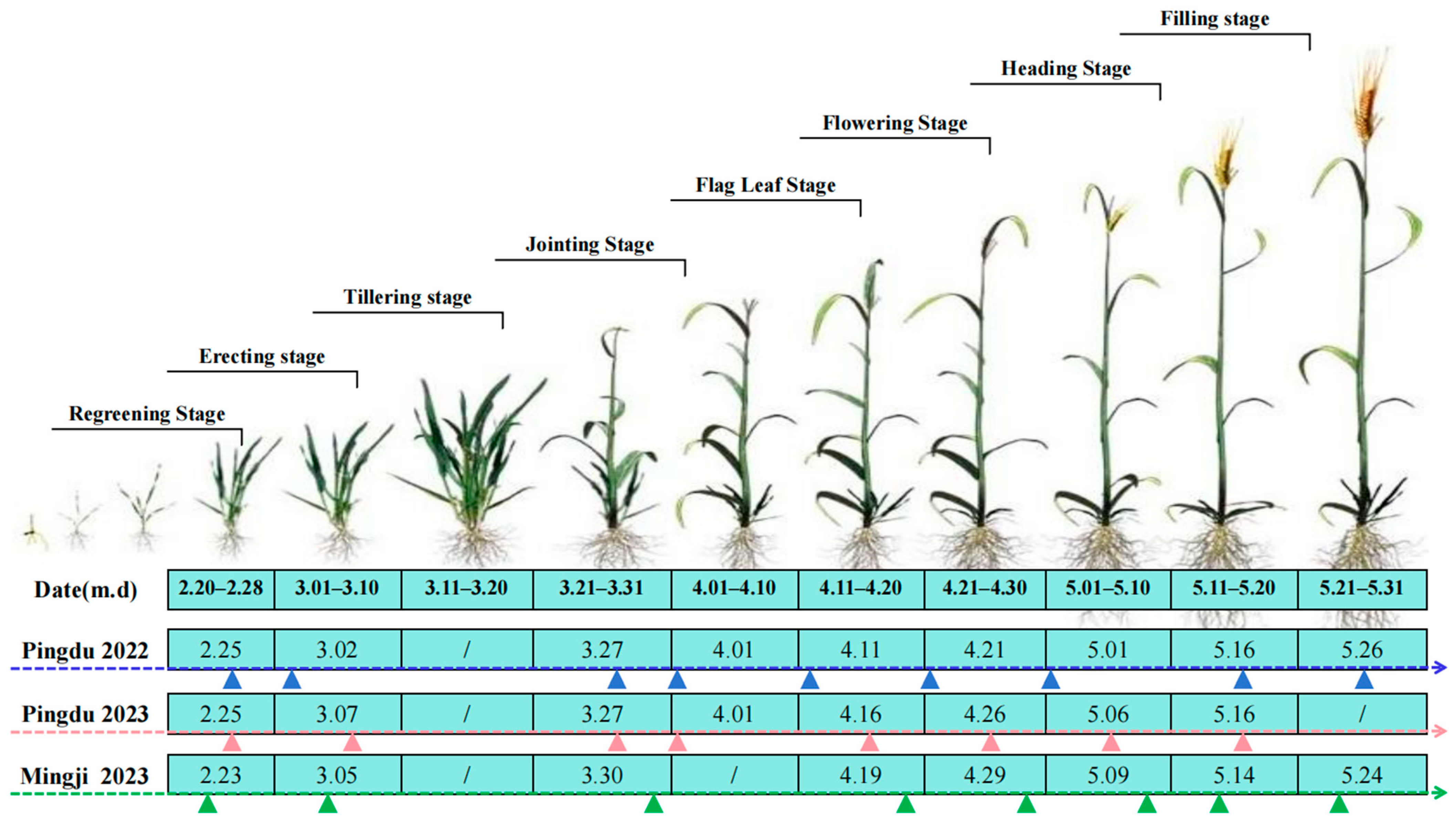
2.2.2. Division of Growth Stages

Image acquisition was carried out as far as possible during the key growth stages of winter wheat after the over-wintering stage. The dates of image acquisition and the corresponding growth stages are shown below (Figure 2).

2.2.3. Measured Data of Winter Wheat Yield

The yield of winter wheat was measured using a sampling method at the wheat harvest stage. First, in the winter wheat field near the sample point, 20–30 rows of wheat were randomly investigated to determine the row spacing, and the number of wheat spikes in 1 m × 9 rows was counted to investigate the number of wheat spikes. At the same time, the wheat spikes were sampled. After drying, the wheat was threshed indoors, and the number of grains per spike, 1000-grain weight, and grain water content were determined by baking. Finally, the yield of winter wheat was calculated according to the three-element method of wheat. The formula is as follows:

$$\mathrm{Yield}=\left(\right(\mathrm{WWS} \times 667 \times \mathrm{KPS} \times \mathrm{TKW})/1000/1000 \times 15)\times \left(100 - \mathrm{SMC}\right) / 87$$

(1)

Here, WWS (ears/m²) is the number of spikes per square meter of winter wheat, KPS (kernels per spike) is the number of grains per spike, TKW (thousand kernel weight, g) is the thousand-grain weight, and SMC (sample moisture content) is the water content of the winter wheat samples.

2.3. Methods

The flow chart of the winter wheat yield prediction model based on RF and the interpolation model (IM) is shown below (Figure 3), which mainly includes four parts:

(1)

Vegetation index screening. This part comprises the comparative analysis of the correlation between five vegetation indexes and yield in the whole growth period and selection of indexes with high correlation in multiple growth periods for modeling the input parameters.

(2)

Model comparison. The missing original time series data and the data optimized by the two IM models are input into the RF model as parameters, and the parameter optimization method with the best prediction yield is selected for modeling by comparing and analyzing the accuracy.

(3)

Screening and combination comparison of winter wheat growth period. The growth period is reduced from 10 periods one by one. The vegetation index of different growth periods and combinations is input into the yield prediction model as a parameter, and the number and combination of growth periods with the best yield estimation effect are obtained by comparing and analyzing the accuracy.

(4)

Prediction yield mapping of winter wheat. The yield prediction results are obtained according to the combined input parameters of the optimal growth period, and the results are transformed into a yield map. Combined with the existing vector map of winter wheat planting area in the study area, the predicted yield map of winter wheat is obtained by pruning.

2.3.1. Calculation of Vegetation Index

According to the canopy spectral characteristics of winter wheat and previous research results, the normalized difference vegetation index (NDVI), the soil-adjusted vegetation index (SAVI), the modified soil-adjusted vegetation index (MSAVI), the enhanced vegetation index (EVI), and the kernel normalized difference vegetation index (kNDVI) were selected for winter wheat yield prediction [8]. The reasons for choosing these five indexes are mainly based on previous studies and their own advantages. During the crop growth period, the photosynthetic active biomass (NDVI) is related to crop yield, but there will be an overfitting phenomenon in some stages [27]. In addition, the SAVI can improve the sensitivity to soil and has a good correlation with yield in the early growth stage of winter wheat [28]. At the same time, the MSAVI is an improvement of the SAVI, and it was proposed to effectively minimize the effect of bare soil without knowing the slope of the soil line [29]. The EVI is designed to optimize the extraction of vegetation signals and to enhance the correction of soil and atmospheric scattering [30]. The kNDVI can handle nonlinear problems better and takes into account the effects of higher-order variations [31] (

Table 2. Vegetation index calculation formulas.

Vegetation Index	Calculation Formula	Reference
NDVI	${(\mathrm{R}}_{\mathrm{nir}}-{\mathrm{R}}_{\mathrm{r}})/({\mathrm{R}}_{\mathrm{nir}}+{\mathrm{R}}_{\mathrm{r}})$	[32]
SAVI	$1.5\times \left({\mathrm{R}}_{\mathrm{nir}}-{\mathrm{R}}_{\mathrm{r}}\right)/{(\mathrm{R}}_{\mathrm{nir}}+{\mathrm{R}}_{\mathrm{r}}+0.5)$	[33]
MSAVI	$0.5\times \left[2 \times {\mathrm{R}}_{\mathrm{nir}}+1-\mathrm{SQRT}{(\left(2 \times {\mathrm{R}}_{\mathrm{nir}}+1\right)}^2-8 \times \left({\mathrm{R}}_{\mathrm{nir}}-{\mathrm{R}}_{\mathrm{r}}\right))\right]$	[34]
EVI	$2.5 \times \left({\mathrm{R}}_{\mathrm{nir}}-{\mathrm{R}}_{\mathrm{r}}\right)/{(\mathrm{R}}_{\mathrm{nir}}+6 {\mathrm{R}}_{\mathrm{r}}-7.5 \times {\mathrm{R}}_{\mathrm{b}}+1)$	[35]
kNDVI	$\tanh \left\{{\left[\left({\mathrm{R}}_{\mathrm{nir}}-{\mathrm{R}}_{\mathrm{r}}\right)/2 \times \sigma \right]}^2\right\}$	[36]

Note: $R_{nir}{ , R}_r \mathrm{and} R_b$ represent the reflectance of the near-infrared band, red band, and blue band, respectively. $\mathsf{\sigma }$ is a length-scale parameter to be specified in each particular application and represents the sensitivity of the index to sparsely/densely vegetated regions.

).

2.3.2. Interpolation Models

The interpolation model (IM) is a numerical analysis method used to estimate the values of unknown points between a given set of discrete data points. The values at these unknown points are inferred by using the information between known data points. The time series curve optimized and enhanced by the interpolation model plays a great role in improving the performance of machine learning [37]. In this study, the vegetation index of the sample point was extracted from the available satellite image, and the missing growth stage was processed using piecewise linear interpolation (PLI) and cubic spline interpolation (CSI) to obtain the vegetation index of all the growth stages of the sample point for the construction of the yield estimation model, which can solve the problem of image loss caused by weather with certainty. When there is no image of one of the ten time phases, the value of the middle day of this time phase is obtained using the interpolation method. Using traditional methods, images with too much cloud cover are generally processed via cloud removal, or other satellite images replace the images with missing dates [18]. These methods may produce some errors due to the resolution of different data sources. Therefore, using the IM to fit and interpolate the optimized data is feasible. The specific methods are as follows:

(1)

PLI: Piecewise linear interpolation uses a linear function to interpolate between adjacent data points. Compared with more complex interpolation methods, PLI is simpler, more intuitive, easier to understand and implement, and is suitable for some data smoothing and approximate scenarios [38]. First, the given data point set is divided into several intervals. Then, in each interval of stages containing missing images, a linear function is used to connect adjacent data points to form a linear curve. The specific formula is as follows:

$$V{I}_X=\frac{(D_X-D_i)(V{I}_{D_{i+1}}-V{I}_{D_i})}{D_{i+1}-D_i}+V{I}_{D_i}$$

(2)

Here, X denotes the middle day of the time phase where the image is missing, ${VI}_X$ is the index value of the interpolation day, $D_X$ is the date of the interpolation day, $D_i$ is the date of the latest image before the interpolation day, $D_{i+1}$ is the date for the latest image after the interpolation day, and ${VI}_{D_i}$ and ${VI}_{D_{i+1}}$ are the index values of the day.

(2)

CSI: Cubic spline interpolation is a more complex interpolation method, which fits cubic polynomials between adjacent data points. Compared with PLI, CSI introduces higher-order polynomials in the fitting process to obtain smoother curves, which is more in line with the time series law of vegetation index [39]. First, the given data point set is divided into several intervals (interpolation is performed between every two dates where an image exists with an interval of 0.05), and then in each interval, the cubic polynomial is used to fit the adjacent data points to ensure that the adjacent intervals are smooth and continuous. The specific formula is as follows:

$$S_i\left(D\right)=a_i(D-D_i{)}^3+b_i(D-D_i{)}^2+c_i(D-D_i)+d_i$$

(3)

$$S_i\left(D_i\right)=V{I}_i$$

(4)

$$S_{i+1}\left(D_{i+1}\right)=V{I}_{i+1}$$

(5)

$$S″\left(D_0\right)=S″\left(D_n\right)=0$$

(6)

where $S_i\left(D\right)$ is a cubic spline function on interval $(D_i$, $D_{i+1}$); $a_i$, $b_i$, $c_i,$ and $d_i$ are coefficients and need to meet the conditions of Equations (5), (6) and (7). $D_i$ and $D_{i+1}$ are the dates of the previous day and the next day to be interpolated; ${VI}_i$ and ${VI}_{i+1}$ are the index values of the corresponding dates; and $D_0$ and $D_n$ are the dates of the two endpoints of the whole vegetation index time series curve, respectively.

The data optimized by each interpolation method were predicted ten times, and each time, the data were randomly divided into a training set and a validation set according to 3:1.

2.3.3. Random Forest

The random forest (RF) model is a type of machine learning algorithm. This model is an integrated learning method. RF involves model integration based on decision tree construction, and regression prediction is performed by constructing multiple decision trees and combining their prediction results [18,35,40]. Each decision tree is trained independently and constructed by the random sampling and feature selection of data. At each split node, the random forest selects the best split feature from the feature set. This randomness helps to reduce the variance of the model and improve the generalization ability [41]. The model adopts the method of sampling back, and the prediction results of each tree are averaged, which is widely used in regression tasks. To model the relationship between VI and winter wheat yield at different growth stages and combinations in this study, the following RF model was established:

(1)

The 10 growth stages were deleted one by one, and the data combinations of different growth stages were exhausted. The yield model was constructed, and the time phase information was analyzed to predict the yield. Finally, 9 growth stages (10 models), 8 growth stages (45 models), 7 growth stages (120 models), 6 growth stages (210 models), 5 growth stages (252 models), 4 growth stages (210 models), 3 growth stages (120 models), 2 growth stages (45 models), and 1 growth stage (10 models) were randomly selected, with a total of 1,023 models. The accuracies of the winter wheat yield estimation model with each combination as the input parameter were compared to obtain the results of all the different situations.

(2)

The data were randomly divided into training and validation sets according to the ratio of 3:1. In the range from 50 to 1000, every 50 was the number of decision trees, and a prediction was made, and the number of decision trees with the best prediction effect was selected. The number of decision trees selected in the RF model was 20.

(3)

The RF model was established with the optimal number of decision trees, and the input parameters were trained and verified to obtain the predicted yield.

2.3.4. Evaluation of Model Accuracy

To carry out scientific model accuracy evaluation and modeling effect comparison, this study used the coefficient of determination (R²), root mean square error (RMSE), normalized root mean square error (NRMSE), and Akaike information criterion (AIC) as the evaluation criteria for model screening and yield estimation model accuracy [42]; these are shown in Equations (7)–(10). The AIC is a statistical criterion for model selection. The main idea is to comprehensively consider the fitting degree and model complexity when evaluating a model to balance the trade-off between data fitting and model simplicity. This model selection method is widely used in fields such as statistical modeling and machine learning to improve the generalization performance of a model.

$$R^2=\frac{{\displaystyle \sum _{i=1}^{\mathrm{n}}}{\left(X_i-\overline{X}\right)}^2{\left(Y_i-\overline{Y}\right)}^2}{n{\displaystyle \sum _{i=1}^n}{\left(X_i-\overline{X}\right)}^2{\displaystyle \sum _{i=1}^n}{\left(Y_i-\overline{Y}\right)}^2}$$

(7)

$$RMSE=SQRT\frac{{\displaystyle \sum _{i=1}^{\mathrm{n}}}{\left(Y_i-X_i\right)}^2}{n}$$

(8)

$$NRMSE=\frac{RMSE}{\overline{X}}$$

(9)

$$AIC=\frac{2\times B-2\times L}{K}$$

(10)

Here, n is the number of samples; $X_i$, $\overline{X}$, $Y_i$, and $\overline{Y}$ represent the measured values, the mean of the measured values, the predicted values, and the mean of the predicted values, respectively. B is the number of independent variables of the model, L is the maximum likelihood function value, and K is the number of samples. Generally, the higher (lower) R² is, the lower (higher) the RMSE is, and the (lower) higher the accuracy of the model is. At the same time, the model with the smallest AIC value is considered a better model.

3. Results

3.1. Vegetation Index Screening

The correlation between the vegetation index and the measured yield of winter wheat in the key growth stage of the study area was analyzed (Figure 4). The results showed that from late February to mid-April, the correlation between the NDVI, the EVI, the MSAVI, the SAVI, the kNDVI, and the yield gradually increased with the advancement of the growth stage, and the maximum correlations corresponding to each index also appeared, which were 0.41, 0.39, 0.32, 0.33, and 0.41, respectively. From mid-April to late May, the correlation decreased and fluctuated with the growth stage, and the vegetation index was negatively correlated with the yield in late May, mainly due to the yellowing of leaves. According to the analysis of different vegetation indexes, the EVI in late February, early March, mid-March, late March, and mid-May had a high correlation with the yield. The MSAVI had the highest correlation with the yield in early April and late May. The correlation between the NDVI and yield was the highest in mid-April, late April, and early May. In each phase of the whole growth period of winter wheat, the correlation between the EVI and yield is mostly in the top three, which is better than the other four indexes. This study considers the growth stage and combination that have the greatest influence on the yield prediction of winter wheat during the whole growth period. Therefore, the EVI of each growth stage was selected as the input parameter to construct the winter wheat yield prediction model.

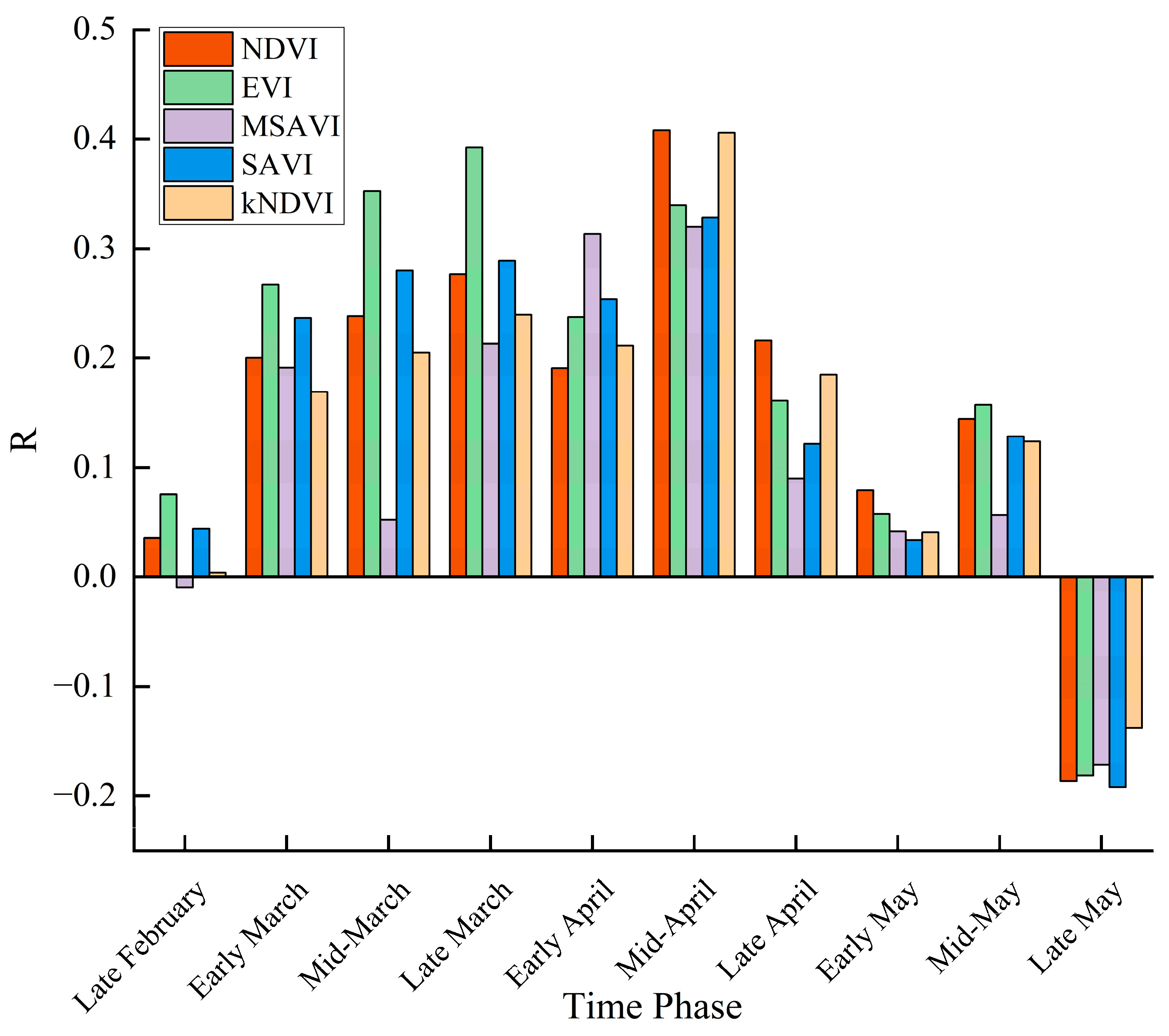
3.2. Correlation between Vegetation Index and Yield in the Study Area

According to the PLI method and the CSI method, the obtained time series images were interpolated, and the EVI values of the sample points at all the growth stages were obtained, which are EVI_PLI and EVI_CSI, respectively, to construct the RF yield estimation model with non-interpolation EVI (EVI_{No Inter}), EVI_PLI, and EVI_CSI as model input variables. The results (Figure 5) show that, in general, the three RF models have good accuracy, and the R² is above 0.68 (Figure 5a). The RF model with EVI_CSI as the input variable (RF-CSI) had the best accuracy in the modeling set and the validation set, with an R² and an RMSEv of 0.75 and 1489 kg/ha, respectively. The RF model with EVI_PLI as the input variable (RF-PLI) has the second-highest accuracy in the modeling set and the validation set, with an R² and an RMSEv of 0.73 and 1581 kg/ha, respectively. The RF model with EVI_{No Inter} as the input variable (RF-No Inter) had the worst accuracy in the modeling set and the validation set, with an R² and an RMSEv of 0.72 and 1689 kg/ha, respectively. RF-CSI therefore has the best effect on estimating winter wheat yield during the whole growth period.

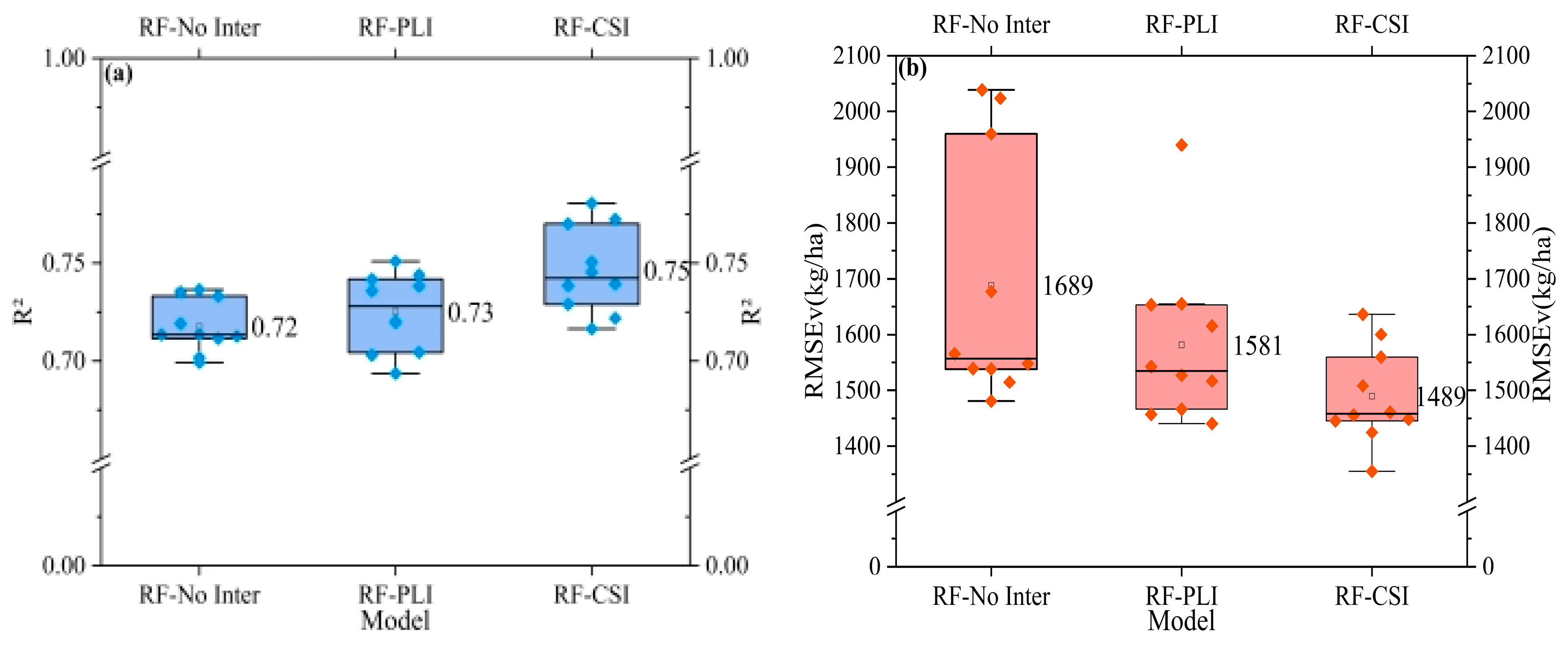
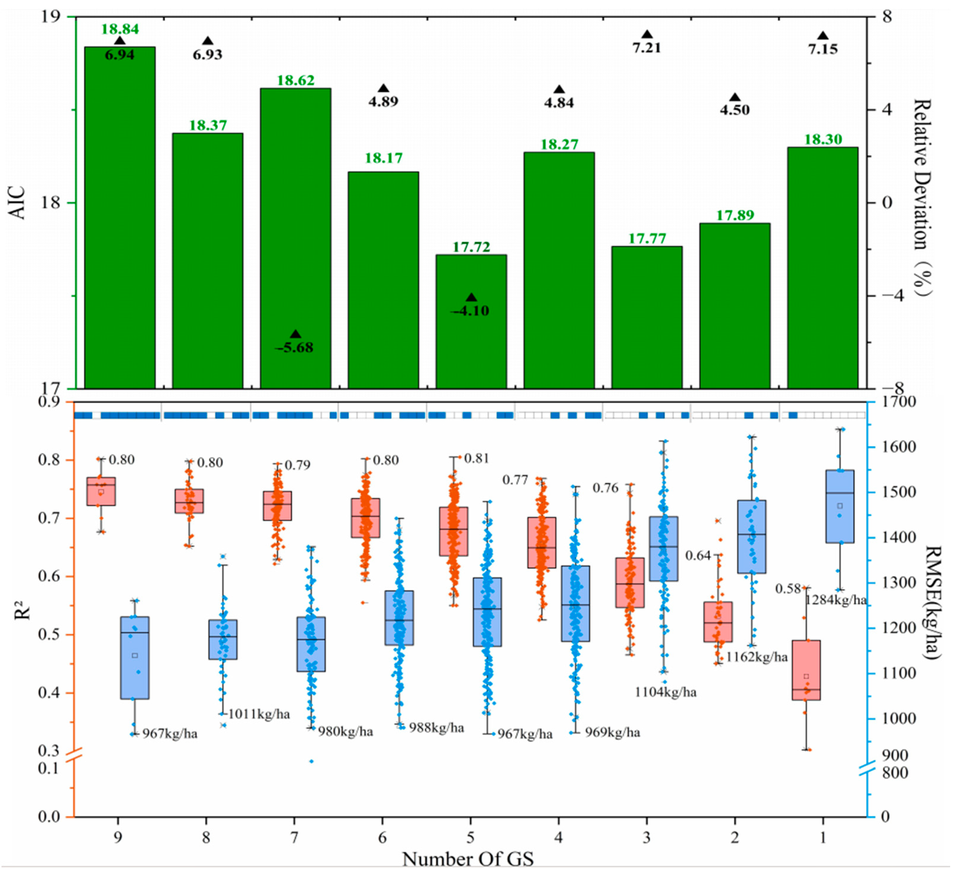
3.3. Time Phase Selection and Model Evaluation of Yield Estimation Using Remote Sensing

The yield estimation models constructed in different growth stages were analyzed (Figure 6). From the perspective of model accuracy and error, with the decrease in growth stage, the R² showed a trend of decreasing slightly first, and then rising, and finally decreasing sharply, and an inflection point appeared when the variable was five growth stages. The RMSE first changed from small fluctuations to a rapid increase, and an inflection point appeared when the variable was four growth stages. Therefore, when the number of input growth stages is less than five, the accuracy of the yield estimation model will decrease. The highest R² and lowest RMSE values of the best yield prediction results from one growth stage to four growth stages are 0.58 and 1284 kg/ha (1GS), 0.64 and 1162 kg/ha (2GS), 0.76 and 1104 kg/ha (3GS), 0.77 and 969 kg/ha (4GS), respectively. When the number of growth stages is lower, it is not conducive to the construction of a winter wheat yield estimation model. When the number of growth stages is greater than or equal to five, the accuracy of the model will fluctuate; the highest R² and lowest RMSE values are 0.80 and 967 kg/ha (9GS), 0.80 and 1011 kg/ha (8GS), 0.79 and 980 kg/ha (7GS), 0.80 and 988 kg/ha (6GS), and 0.81 and 967 kg/ha (5GS). The lowest NRMSE obtained by the optimal combination of five fertility periods as a parameter input is 15% (Figure 7). As a result, when the number of growth stages is five, the accuracy of the yield estimation model is the highest.

Considering the complexity of the model, the results of the AIC of the different input variables were analyzed (Figure 6). The value of the AIC was obtained by selecting the combination with the highest R² for different numbers of growth stages. The AIC value obtained by taking the five growth stages as the input variables is the lowest, and the AIC value is 17.72. The AIC results with three fertility stages and two fertility stages as input variables were 17.77 and 17.89, respectively. The values for the other input variables are higher than 18; therefore, the complexity of the yield estimation model is the best when the number of fertility stages is five.

The relative deviation of yield prediction using different growth stage combinations was further analyzed (Figure 6). The absolute value of relative deviation is less than 5% when the input variables are eight, six, five, and four growth stages, and the minimum relative deviation is −4.10% for five growth stages. The relative deviation of the number and combination of other input variables is greater than 5%, and the maximum is 7.21% for seven growth stages, followed by 7.15% for nine growth stages. In addition, when the input variables are two and one growth stages, the relative deviations are 6.93% and 6.94%, respectively.

Through the comprehensive comparison of these results, when the number of growth stages is too high or too low, the accuracy of the model to predict the yield of winter wheat will be reduced, and the prediction effect of winter wheat yield using five growth stages is the best. The dispersion of the validation set is good, and the accuracy reaches a very significant level, and there is no saturation phenomenon, indicating that the screening of a combination of growth stages is scientific and correct, and a better yield prediction result can be obtained after they are input into the model (Figure 7). When the number of growth stages is five, the best combination of R² is data from late February, early March, early April, mid-May, and late May.

3.4. Production Remote Sensing Mapping and Analysis

Through the comparison and evaluation of these modeling results, the RF-CSI model has the best winter wheat yield prediction accuracy when the input variables are the five phases of late February, early March, early April, mid-May, and late May. Based on RF-CSI_5GS mapping, the yield prediction results of the Pingdu study area in 2022 (Figure 8a) and 2023 (Figure 8b) and the Mingji Town study area in 2023 (Figure 8c) were obtained. In general, the yield of the study area in 2022 is higher than that in 2023, and the yield is more than 9000 kg/ha, accounting for 58.17%, with an average yield of 9180 kg/ha. In 2023, the overall yield of the Pingdu study area decreased, and the yield was in the range of 7000–8000 kg/ha, accounting for 45.09%, with an average yield of 7254 kg/ha. By contrast, the yield of the study area in Mingji Town in 2023 is relatively good. The area with a yield greater than 9000 kg/ha represents the majority, accounting for 62.03%, and the average yield is 9050 kg/ha.

4. Discussion

4.1. Effect of Vegetation Index Selection on Yield Estimation Model

In this study, we compared the correlation between five vegetation indices, the NDVI, the EVI, the MSAVI, the SAVI, the kNDVI, and winter wheat yield, in the whole growth period. The results have certain differences in different growth stages. The final selected EVI has a high correlation with the yield in multiple growth periods, consistent with the previous studies. The EVI is derived from the SAVI and the atmospherically resistant vegetation index, which are more sensitive in high-biomass areas and improve the vegetation detection ability by reducing the atmospheric effect and decoupling the background signal of the vegetation canopy. The EVI not only has better sensitivity to the yield, but also minimizes the impact of soil information [35]. The EVI is more important than several other vegetation indices for yield prediction, mainly because the EVI can better reflect phenological characteristics. The previous studies have mostly used the NDVI to predict yield, but NDVI saturation occurs under high-biomass conditions, affecting the accuracy of yield prediction in some key yield estimation growth periods [43,44,45]. Other crop studies have also confirmed that a rice yield estimation model based on the EVI is better than a rice yield estimation model based on the NDVI [46]; because the EVI is calculated based on the blue wavelength, the influence of aerosols on the red wavelength is eliminated, and the accuracy of maize yield prediction is improved [47]. As an optimization index, the EVI uses the canopy signal to enhance the vegetation signal and better show the difference in vegetation canopy density [47,48].

4.2. Consideration and Influence of Data Interpolation in Yield Estimation

In this study, the EVI time series curve optimized by the CSI had the best effect on predicting winter wheat yield using the model. Compared with the PLI, the CSI can achieve more accurate interpolation, its curve is smoother, and its adaptability to data time series is stronger. The previous studies have also proved that the spline interpolation method is the best interpolation method for meteorological element interpolation [49]. Therefore, the CSI method makes our research more accurate in predicting regional wheat yield. Evans et al. used the spline interpolation method to smooth the data curve in their study for the subsequent winter wheat yield prediction [50]. Some studies have used interpolation to process data to obtain a coherent, complete dataset to predict the extreme yield loss of crops [51]. In addition, the grid surface generated by the spline is usually smoother than the grid surface generated by other interpolation techniques, helping to visually interpret the results [52]. This shows that the data obtained by the spline interpolation method are more reliable. In addition to the machine learning model, the multi-source data in the crop growth model can also be optimized by the spline interpolation method, and then input into the model to improve the yield prediction accuracy [53]. Therefore, the CSI can well maintain the smoothness and continuity of data and reduce the loss of information; this also does not require the a priori estimation of the spatial autocorrelation structure and the regular distribution of data points [54,55].

4.3. Analysis of the Influence of Time Phase Selection on Yield Estimation Model in Yield Prediction

Compared with LUE, a DA model, and ESMs, the winter wheat yield prediction model based on RF can simplify and realize a complex experimental study that takes the quantity and combination of EVIs in different growth stages as an input. Combined with historical production data, the results of different input parameters can be better reflected.

This study shows that the selection of EVIs at some key growth stages as input parameters can improve the yield estimation accuracy of the winter wheat yield estimation model based on RF. This is because in the whole growth process of winter wheat, the vegetation index cannot easily have a good correlation with the yield, mainly because from the beginning of the winter wheat dormancy stage to the harvest stage, droughts, freezing injuries, pests, lodging, and other phenomena will lead to changes in the yield [44,56]. Therefore, selecting the growth stage with a high correlation with the yield is conducive to a more accurate estimation of the yield. When the number of input growth stages is different, the accuracy will be different. When the number of parameters is greater than or equal to five stages, the accuracy of the number of different growth stages as the best time phase combination in the input parameters fluctuates and decreases to some extent, but it tends to be saturated, potentially due to the over-fitting phenomenon when there are too many growth stages. However, when the number of stages is less than five, the accuracy will be greatly reduced. This is because when the amount of information on the growth stage is too little, the prediction ability of the model will be affected because a lack of data is not conducive to the accumulation of entire seasonal information, and the results will be biased [44]. Due to the influence of temperature, rainfall, pesticide deworming, irrigation, and fertilization, the winter wheat vegetation index at different growth stages will change. Furthermore, because of the different complexities of the model with different input parameters, the AIC is used to combine the R² and RMSE for model evaluation (Figure 6).

The accuracy and complexity of the prediction results of the model with a five-stage EVI as input are the best (R² is 0.81, the AIC is 17.72, the relative deviation is −4.10%, and the NRMSE is 15%). The corresponding growth periods are the regreening, erecting, jointing, heading, and filling stages; using too many or too few growth periods will reduce the accuracy of the model. When the number of input crop growth stages is the same, different growth stage combinations will produce different yield prediction accuracies [57]. This is because in the growth and development process of winter wheat, due to the influence of external factors, the potential yields of each growth period are different, that is, the linear correlation between some periods and the final yield are quite different [58]. Therefore, different combinations of time phases yield different R², RMSE, and NRMSE values. When the input growth stage is highly correlated with the final yield, there will be a higher R² or a lower RMSE and NRMSE (Figure 6). The previous studies have found that the accuracy of yield prediction is higher using growth period observation data closer to the harvest date (June) [44,59], verifying the phase selection results of the present study. In addition, relevant studies have shown that the key growth stages with good correlation with winter wheat yield are the jointing, heading, and filling stages [60]. Deng et al. found that the contribution rate of the jointing stage to winter wheat yield prediction was the highest, followed by the erecting, heading, filling, and regreening stages [61]. The estimation of other crops has also confirmed that the rice yield at the jointing and booting stages has a good correlation with multiple spectral indexes. After accumulating the vegetation indexes at multiple growth stages, a yield can be better predicted [62]. These findings indicate the rationality of screening the best growth period for yield prediction and using it as the input parameter of the model.

However, in some cases, the use of multispectral data to forecast winter wheat yield also has certain limitations, and the addition of other data such as meteorological data may have better results [27,63]. In addition, compared with satellite remote sensing, UAV remote sensing has the advantages of high spatial and temporal resolutions, a low cost, flexibility, etc., and has more advantages in small research areas [64].

5. Conclusions

Based on multi-temporal remote sensing data and an interpolation algorithm, this study completed the combination and screening of the optimal prediction growth stages of an RF winter wheat yield estimation model and completed winter wheat yield prediction and mapping in the study area. In this paper, the CSI algorithm was used to optimize the EVI of the growth stage without remote sensing data. The whole growth period is suitable for the yield prediction of winter wheat, and the prediction effect is good. The RF-CSI model that used a five-stage EVI (regreening, erecting, jointing, heading, and filling stages) as input variables had the highest accuracy, with an R² and an RMSE of 0.81 and 1250 kg/ha, respectively. The yield prediction accuracy of the RF-CSI model is higher than those of the RF-PLI model and RF-No Inter model. The RF-CSI model and the yield prediction growth stage obtained via final screening have good application potential in subsequent winter wheat yield estimations and also provide a good method for the yield prediction of other crops. However, this study only uses a machine learning method to predict the yield, and the study area is small. In future work, a different study area and other models can be used to improve the generalization performance of phase selection.

References

1. Alexandratos, N.; Bruinsma, J. World Agriculture towards 2030/2050: The 2012 Revision; FAO: Rome, Italy, 2012. [Google Scholar]
2. Ray, D.K.; Mueller, N.D.; West, P.C.; Foley, J.A. Yield trends are insufficient to double global crop production by 2050. PLoS ONE 2013, 8, e66428. [Google Scholar] [CrossRef]
3. FAO. The State of Food and Agriculture 2022: Transforming Agri-Food Systems with Agricultural Automation; FAO: Rome, Italy, 2022. [Google Scholar]
4. Sun, J.; Lai, Z.; Di, L.; Sun, Z.; Tao, J.; Shen, Y. Multilevel deep learning network for county-level corn yield estimation in the us corn belt. IEEE J. Sel. Top. Appl. Earth Obs. Remote Sens. 2020, 13, 5048–5060. [Google Scholar] [CrossRef]
5. Zhang, H.; Zhang, Y.; Liu, K.; Lan, S.; Gao, T.; Li, M. Winter wheat yield prediction using integrated Landsat 8 and Sentinel-2 vegetation index time-series data and machine learning algorithms. Comput. Electron. Agric. 2023, 213, 108250. [Google Scholar] [CrossRef]
6. Chen, P.; Li, Y.; Liu, X.; Tian, Y.; Zhu, Y.; Cao, W.; Cao, Q. Improving yield prediction based on spatio-temporal deep learning approaches for winter wheat: A case study in Jiangsu Province, China. Comput. Electron. Agric. 2023, 213, 108201. [Google Scholar] [CrossRef]
7. Paudel, D.; Boogaard, H.; de Wit, A.; Janssen, S.; Osinga, S.; Pylianidis, C.; Athanasiadis, I.N. Machine learning for large-scale crop yield forecasting. Agric. Syst. 2021, 187, 103016. [Google Scholar] [CrossRef]
8. Zhao, Y.; Potgieter, A.B.; Zhang, M.; Wu, B.; Hammer, G.L. Predicting wheat yield at the field scale by combining high-resolution Sentinel-2 satellite imagery and crop modelling. Remote Sens. 2020, 12, 1024. [Google Scholar] [CrossRef]
9. Liakos, K.G.; Busato, P.; Moshou, D.; Pearson, S.; Bochtis, D. Machine learning in Agriculture: A review. Sensors 2018, 18, 2674. [Google Scholar] [CrossRef]
10. Zhou, W.; Liu, Y.; Ata-Ul-Karim, S.T.; Ge, Q.; Li, X.; Xiao, J. Integrating climate and satellite Remote Sensing data for predicting county-level wheat yield in China using machine learning methods. Int. J. Appl. Earth Obs. Geoinf. 2022, 111, 102861. [Google Scholar] [CrossRef]
11. Manivasagam, V.S.; Rozenstein, O. Practices for upscaling crop simulation models from field scale to large regions. Comput. Electron. Agric. 2020, 175, 105554. [Google Scholar] [CrossRef]
12. Jeong, J.H.; Resop, J.P.; Mueller, N.D.; Fleisher, D.H.; Yun, K.; Butler, E.E.; Timlin, D.J.; Shim, K.-M.; Gerber, J.S.; Reddy, V.R.; et al. Random forests for global and regional crop yield predictions. PLoS ONE 2016, 11, e0156571. [Google Scholar] [CrossRef]
13. Wang, J.; Wang, P.; Tian, H.; Tansey, K.; Liu, J.; Quan, W. A deep learning framework combining CNN and GRU for improving wheat yield estimates using time series remotely sensed multi-variables. Comput. Electron. Agric. 2023, 206, 107705. [Google Scholar] [CrossRef]
14. Gómez, D.; Salvador, P.; Sanz, J.; Casanova, J.L. Modelling wheat yield with antecedent information, satellite and climate data using machine learning methods in Mexico. Agric. For. Meteorol. 2021, 300, 108317. [Google Scholar] [CrossRef]
15. Breiman, L. Random forests. Mach. Learn. 2001, 45, 5–32. [Google Scholar] [CrossRef]
16. Sun, Y.; Zhang, S.; Tao, F.; Aboelenein, R.; Amer, A. Improving Winter Wheat Yield Forecasting Based on Multi-Source Data and Machine Learning. Agriculture 2022, 12, 571. [Google Scholar] [CrossRef]
17. Han, S.; Zhao, Y.; Cheng, J.; Zhao, F.; Yang, H.; Feng, H.; Li, Z.; Ma, X.; Zhao, C.; Yang, G. Monitoring key wheat growth variables by integrating phenology and UAV multispectral imagery data into random forest model. Remote Sens. 2022, 14, 3723. [Google Scholar] [CrossRef]
18. Fieuzal, R.; Bustillo, V.; Collado, D.; Dedieu, G. Combined use of multi-temporal Landsat-8 and Sentinel-2 images for wheat yield estimates at the intra-plot spatial scale. Agronomy 2020, 10, 327. [Google Scholar] [CrossRef]
19. Li, Z.; Taylor, J.; Yang, H.; Casa, R.; Jin, X.; Li, Z.; Song, X.; Yang, G. A hierarchical interannual wheat yield and grain protein prediction model using spectral vegetative indices and meteorological data. Field Crops Res. 2020, 248, 107711. [Google Scholar] [CrossRef]
20. Segarra, J.; Araus, J.L.; Kefauver, S.C. Farming and Earth Observation: Sentinel-2 data to estimate within-field wheat grain yield. Int. J. Appl. Earth Obs. Geoinf. 2022, 107, 102697. [Google Scholar] [CrossRef]
21. Wang, L.; Tian, Y.; Yao, X.; Zhu, Y.; Cao, W. Predicting grain yield and protein content in wheat by fusing multi-sensor and multi-temporal remote-sensing images. Field Crops Res. 2014, 164, 178–188. [Google Scholar] [CrossRef]
22. Fu, Y.; Huang, J.; Shen, Y.; Liu, S.; Huang, Y.; Dong, J.; Han, W.; Ye, T.; Zhao, W.; Yuan, W. A satellite-based method for national winter wheat yield estimating in China. Remote Sens. 2021, 13, 4680. [Google Scholar] [CrossRef]
23. Jin, H.; Xu, W.; Li, A.; Xie, X.; Zhang, Z.; Xia, H. Spatially and Temporally Continuous Leaf Area Index Mapping for Crops through Assimilation of Multi-resolution Satellite Data. Remote Sens. 2019, 11, 2517. [Google Scholar] [CrossRef]
24. Soltani, A.; Holger, M.; Peter, D.V. Assessing linear interpolation to generate daily radiation and temperature data for use in crop simulations. Eur. J. Agron. 2004, 21, 133–148. [Google Scholar] [CrossRef]
25. Wu, S.; Yang, P.; Ren, J.; Chen, Z.; Li, H. Regional winter wheat yield estimation based on the WOFOST model and a novel VW-4DEnSRF assimilation algorithm. Remote Sens. Environ. 2021, 255, 112276. [Google Scholar] [CrossRef]
26. Li, X.; Zhu, W.; Xie, Z.; Zhan, P.; Huang, X.; Sun, L.; Duan, Z. Assessing the effects of time interpolation of NDVI composites on phenology trend estimation. Remote Sens. 2021, 13, 5018. [Google Scholar] [CrossRef]
27. Vannoppen, A.; Gobin, A. Estimating Farm Wheat Yields from NDVI and Meteorological Data. Agronomy 2021, 11, 946. [Google Scholar] [CrossRef]
28. Nagy, A.; Szabó, A.; Adeniyi, O.D.; Tamás, J. Wheat yield forecasting for the Tisza River catchment using landsat 8 NDVI and SAVI time series and reported crop statistics. Agronomy 2021, 11, 652. [Google Scholar] [CrossRef]
29. Yunus, K.; Polat, N.A. linear approach for wheat yield prediction by using different spectral vegetation indices. Int. J. Eng. Geosci. 2023, 8, 52–62. [Google Scholar]
30. Kouadio, L.; Newlands, N.K.; Davidson, A.; Zhang, Y.; Chipanshi, A. Assessing the performance of MODIS NDVI and EVI for seasonal crop yield forecasting at the ecodistrict scale. Remote Sens. 2014, 6, 10193–10214. [Google Scholar] [CrossRef]
31. Wang, Q.; Moreno-Martínez, Á.; Muñoz-Marí, J.; Campos-Taberner, M.; Camps-Valls, G. Estimation of vegetation traits with kernel NDVI. ISPRS J. Photogramm. Remote Sens. 2023, 195, 408–417. [Google Scholar] [CrossRef]
32. Rouse, J.W.; Haas, R.H.; Schell, J.A.; Deering, D.M. Monitoring vegetation systems in the Great Plains with ERTS. NASA Spec. Publ. 1974, 351, 309. [Google Scholar]
33. Huete, A.R. A soil-adjusted vegetation index (SAVI). Remote Sens. Environ. 1988, 25, 295–309. [Google Scholar] [CrossRef]
34. Qi, J.; Chehbouni, A.; Huete, A.R.; Kerr, Y.H.; Sorooshian, S. A modified soil adjusted vegetation index. Remote Sens. Environ. 1994, 48, 119–126. [Google Scholar] [CrossRef]
35. Huete, A.; Didan, K.; Miura, T.; Rodriguez, E.P.; Gao, X.; Ferreira, L.G. Overview of the radiometric and biophysical performance of the MODIS vegetation indices. Remote Sens. Environ. 2002, 83, 195–213. [Google Scholar] [CrossRef]
36. Camps-Valls, G.; Campos-Taberner, M.; Moreno-Martínez, A.; Walther, S.; Duveiller, G.; Cescatti, A.; Mahecha, M.D.; Muñoz-Marí, J.; García-Haro, F.J.; Guanter, L.; et al. A unified vegetation index for quantifying the terrestrial biosphere. Sci. Adv. 2021, 7, eabc7447. [Google Scholar] [CrossRef]
37. Oh, C.; Han, S.; Jeong, J. Time-series data augmentation based on interpolation. Procedia Comput. Sci. 2020, 175, 64–71. [Google Scholar] [CrossRef]
38. Kodama, K.M.; Kourkchi, E.; Longman, R.J.; Lucas, M.P.; Bateni, S.M.; Huang, Y.F.; Kagawa-Viviani, A.; Mclean, J.; Cleveland, S.B.; Giambelluca, T.W. Mapping Daily Air Temperature Over the Hawaiian Islands From 1990 to 2021 via an Optimized Piecewise Linear Regression Technique. Earth Space Sci. 2024, 11, e2023EA002851. [Google Scholar] [CrossRef]
39. Wu, Y.H.; Hung, M.C.; Patton, J. Assessment and visualization of spatial interpolation of soil pH values in farmland. Precis. Agric. 2013, 14, 565–585. [Google Scholar] [CrossRef]
40. Wang, L.; Zhou, X.; Zhu, X.; Dong, Z.; Guo, W. Estimation of biomass in wheat using random forest regression algorithm and Remote Sensing data. Crop J. 2016, 4, 212–219. [Google Scholar] [CrossRef]
41. Everingham, Y.; Sexton, J.; Skocaj, D.; Inman-Bamber, G. Accurate prediction of sugarcane yield using a random forest algorithm. Agron. Sustain. Dev. 2016, 36, 27. [Google Scholar] [CrossRef]
42. Wang, X.; Huang, J.; Feng, Q.; Yin, D. Winter wheat yield prediction at county level and uncertainty analysis in main wheat-producing regions of China with deep learning approaches. Remote Sens. 2020, 12, 1744. [Google Scholar] [CrossRef]
43. Han, J.; Zhang, Z.; Cao, J.; Luo, Y.; Zhang, L.; Li, Z.; Zhang, J. Prediction of winter wheat yield based on multi-source data and machine learning in China. Remote Sens. 2020, 12, 236. [Google Scholar] [CrossRef]
44. Naqvi, S.; Tahir, M.N.; Shah, G.A.; Sattar, R.S.; Awais, M. Remote estimation of wheat yield based on vegetation indices derived from time series data of Landsat 8 imagery. Appl. Ecol. Environ. Res. 2019, 17, 3909–3925. [Google Scholar] [CrossRef]
45. Agapiou, A.; Hadjimitsis, D.G.; Alexakis, D.D. Evaluation of broadband and narrowband vegetation indices for the identification of archaeological crop marks. Remote Sens. 2012, 4, 3892–3919. [Google Scholar] [CrossRef]
46. Son, N.; Chen, C.; Minh, V.; Trung, N. A comparative analysis of multitemporal MODIS EVI and NDVI data for large-scale rice yield estimation. Agric. For. Meteorol. 2014, 197, 52–64. [Google Scholar] [CrossRef]
47. Jin, X.; Li, Z.; Feng, H.; Ren, Z.; Li, S. Estimation of maize yield by assimilating biomass and canopy cover derived from hyperspectral data into the AquaCrop model. Agric. Water Manag. 2020, 227, 105846. [Google Scholar] [CrossRef]
48. Jin, X.; Li, Z.; Yang, G.; Yang, H.; Feng, H.; Xu, X.; Wang, J.; Li, X.; Luo, J. Winter wheat yield estimation based on multi-source medium resolution optical and radar imaging data and the AquaCrop model using the particle swarm optimization algorithm. ISPRS J. Photogramm. Remote Sens. 2017, 126, 24–37. [Google Scholar] [CrossRef]
49. Lv, Z.; Liu, X.; Cao, W.; Zhu, Y. A model-based estimate of regional wheat yield gaps and water use efficiency in main winter wheat production regions of China. Sci. Rep. 2017, 7, 6081. [Google Scholar] [CrossRef]
50. Evans, F.H.; Shen, J. Long-term hindcasts of wheat yield in fields using remotely sensed phenology, climate data and machine learning. Remote Sens. 2021, 13, 2435. [Google Scholar] [CrossRef]
51. Ben-Ari, T.; Adrian, J.; Klein, T.; Calanca, P.; Van der Velde, M.; Makowski, D. Identifying indicators for extreme wheat and maize yield losses. Agric. For. Meteorol. 2016, 220, 130–140. [Google Scholar] [CrossRef]
52. Eyre, R.; Lindsay, J.; Laamrani, A.; Berg, A. Within-Field Yield Prediction in Cereal Crops Using LiDAR-Derived Topographic Attributes with Geographically Weighted Regression Models. Remote Sens. 2021, 13, 4152. [Google Scholar] [CrossRef]
53. Mo, X.; Liu, S.; Lin, Z.; Xu, Y.; Xiang, Y.; McVicar, T. Prediction of crop yield, water consumption and water use efficiency with a SVAT-crop growth model using remotely sensed data on the North China Plain. Ecol. Model. 2005, 183, 301–322. [Google Scholar] [CrossRef]
54. Van, W.J.; Grassini, P.; Cassman, K.G. Impact of derived global weather data on simulated crop yields. Glob. Change Biol. 2013, 19, 3822–3834. [Google Scholar]
55. Lv, Z.; Liu, X.; Cao, W.; Zhu, Y. Climate change impacts on regional winter wheat production in main wheat production regions of China. Agric. For. Meteorol. 2013, 171–172, 234–248. [Google Scholar] [CrossRef]
56. Raun, W.R.; Solie, J.B.; Johnson, G.V.; Stone, M.L.; Lukina, E.V.; Thomason, W.E.; Schepers, J.S. In-season prediction of potential grain yield in winter wheat using canopy reflectance. Agron. J. 2001, 93, 131–138. [Google Scholar] [CrossRef]
57. Ren, Y.; Li, Q.; Du, X.; Zhang, Y.; Wang, H.; Shi, G.; Wei, M. Analysis of corn yield prediction potential at various growth phases using a process-based model and deep learning. Plants 2023, 12, 446. [Google Scholar] [CrossRef] [PubMed]
58. Yu, H.; Zhang, Q.; Sun, P.; Song, C. Impact of droughts on winter wheat yield in different growth stages during 2001–2016 in Eastern China. Int. J. Disaster Risk Sci. 2018, 9, 376–391. [Google Scholar] [CrossRef]
59. Özdoğan, M. Modeling the impacts of climate change on wheat yields in Northwestern Turkey. Agric. Ecosyst. Environ. 2011, 141, 1–12. [Google Scholar] [CrossRef]
60. Zhang, Y.; Qin, Q.; Ren, H.; Sun, Y.; Li, M.; Zhang, T.; Ren, S. Optimal hyperspectral characteristics determination for winter wheat yield prediction. Remote Sens. 2018, 10, 2015. [Google Scholar] [CrossRef]
61. Deng, Q.; Wu, M.; Zhang, H.; Cui, Y.; Li, M.; Zhang, Y. Winter Wheat Yield Estimation Based on Optimal Weighted Vegetation Index and BHT-ARIMA Model. Remote Sens. 2022, 14, 1994. [Google Scholar] [CrossRef]
62. Zhou, X.; Zheng, H.B.; Xu, X.Q.; He, J.Y.; Ge, X.K.; Yao, X.; Cheng, T.; Zhu, Y.; Cao, W.X.; Tian, Y.C. Predicting grain yield in rice using multi-temporal vegetation indices from UAV-based multispectral and digital imagery. ISPRS J. Photogramm. Remote Sens. 2017, 130, 246–255. [Google Scholar] [CrossRef]
63. Li, Z.; Fan, C.; Zhao, Y.; Jin, X.; Casa, R.; Huang, W.; Song, X.; Blasch, G.; Yang, G.; Taylor, J.; et al. Remote sensing of quality traits in cereal and arable production systems: A review. The Crop J. 2024, 12, 45–57. [Google Scholar] [CrossRef]
64. Yang, S.; Hu, L.; Wu, H.; Ren, H.; Qiao, H.; Li, P.; Fan, W. Integration of crop growth model and random forest for winter wheat yield estimation from UAV hyperspectral imagery. IEEE J. Sel. Top. Appl. Earth Obs. Remote Sens. 2021, 14, 6253–6269. [Google Scholar] [CrossRef]
Figure 1. The location of study area and distribution of sample points ((a): China. (b): Shandong Province. The blue part of this figure represents study area 1 in Mingji Town, and the red part represents study area 2 in Pingdu City. (c): Study area 1. The blue dots represent the sample points. (d): Study area 2. The blue dots represent the sample points in 2023, and the red dots represent the sample points in 2022).
Remotesensing 16 01995 g001
Figure 2. Growth period of winter wheat (the number represents the date when the image was obtained). M is month, and d is day.
Remotesensing 16 01995 g002
Figure 3. Flow chart of RF-IM model (PLI: piecewise linear interpolation; CSI: cubic spline interpolation).
Remotesensing 16 01995 g003
Figure 4. Correlation between vegetation index and yield in the study area.
Remotesensing 16 01995 g004
Figure 5. R2 (a) and RMSEv (b) of winter wheat yield estimation model after optimizing time series data using different interpolation models. (RF-No Inter: random forest with non-interpolation time series; RF-PLI: random forest combined with time series optimized by piecewise linear interpolation; RF-CSI: random forest of time series combined with cubic spline interpolation optimization; RMSEv is the RMSE of the validation set).
Remotesensing 16 01995 g005
Figure 6. Growth stage screening box plot and AIC histogram (black triangle is relative deviation = (predicted mean − measured mean)/measured mean). The predicted and measured values are the validation dataset. The green histogram is the AIC value. The blue and white grid above the box line graph is the optimal combination method when the number of different growth stages is input as a parameter, from the first cell on the left to the tenth cell, representing the time phase. The red box line diagram is the R2 value; the blue box line graph is the RMSE value.
Remotesensing 16 01995 g006
Figure 7. Validation results of winter wheat yield prediction model at five growth stages (the blue points are the training set, and the red points are the verification set. Note: the asterisk in this figure indicates that the correlation is extremely significant (p < 0.01)).
Remotesensing 16 01995 g007
Figure 8. Winter wheat yield distribution in the study area ((a): Pingdu City in 2022; (b): Pingdu City in 2023; (c): Mingji Town in 2023).
Remotesensing 16 01995 g008