Trends of Key Greenhouse Gases as Measured in 2009–2022 at the FTIR Station of St. Petersburg State University

Abstract

Key long-lived greenhouse gases (CO₂, CH₄, and N₂O) are perhaps among the best-studied components of the Earth’s atmosphere today; however, attempts to predict or explain trends or even shorter-term variations of these trace gases are not always successful. Infrared spectroscopy is a recognized technique for the ground-based long-term monitoring of the gaseous composition of the atmosphere. The current paper is focused on the analysis of new data on CO₂, CH₄, and N₂O total columns (TCs) retrieved from high resolution IR solar spectra acquired during 2009–2022 at the NDACC atmospheric monitoring station of St. Petersburg State University (STP station, 59.88°N, 29.83°E, 20 m asl.). The paper provides information on the FTIR system (Fourier-transform infrared) installed at the STP station, and an overview of techniques used for the CO₂, CH₄, and N₂O retrievals. Trends of key greenhouse gases and their confidence levels were evaluated using an original approach which combines the Lomb–Scargle method with the cross-validation and bootstrapping techniques. As a result, the following fourteen-year (2009–2022) trends of TCs have been revealed: (0.56 ± 0.01) % yr⁻¹ for CO₂; (0.46 ± 0.02) % yr⁻¹ for CH₄; (0.28 ± 0.01) % yr⁻¹ for N₂O. A comparison with trends based on the EMAC numerical modeling data was carried out. The trends of greenhouse gases observed at the STP site are consistent with the results of the in situ monitoring performed at the same geographical location, and with the independent estimates of the global volume mixing ratio growth rates obtained by the GAW network and the NOAA Global Monitoring Laboratory. There is reasonable agreement between the CH₄ and N₂O TC trends for 2009–2019, which have been derived from FTIR measurements at three locations: the STP site, Izaña Observatory and the University of Toronto Atmospheric Observatory.

1. Introduction

Carbon dioxide (CO₂), methane (CH₄), and nitrous oxide (N₂O) are the key long-lived greenhouse gases (LLGHGs), which have contributed to about 89% of the increase in global radiative forcing from the pre-industrial times [1]. Radiative forcing by LLGHGs increased by 49% from 1990 to 2021, with carbon dioxide accounting for about 80% of that increase [2]. An analysis of the latest data from the GAW WMO (Global Atmosphere Watch, the World Meteorological Organization) observational network revealed that the mixing ratios of carbon dioxide, methane and nitrous oxide in the atmosphere continue to reach the new maximums. The globally averaged surface mixing ratios of LLGHGs observed in 2021 amounted to 415.7 ± 0.2 ppm, 1908 ± 2 ppb, 334.5 ± 0.1 ppb for CO₂, CH₄, and N₂O, respectively [1]. These three greenhouse gases are perhaps among the best-studied components of the Earth’s atmosphere today [3]. Basic information on their importance, atmospheric lifetime and major global sources and sinks is given in

Table 1. General information on investigated long-lived greenhouse gases (GHGs).

Chemical Formula and Name	Importance	Atmospheric Lifetime	Main Global Sources and Sinks
CH4, methane	Long-lived GHG, responsible for 16% of the radiative forcing, Global Warming Potential (100 years) GWP = 27–30 [3,16]; CH4 decay leads to the formation of tropospheric O3 and stratospheric H2O [1]	9–12 years [1,17]	Sources: natural wetlands, agriculture and waste, fossil fuels, biomass burning [5]; 50–65% of total emissions come from human activities [3]. Sinks: chemical loss by OH oxidation, soil uptake [5]
CO2, carbon dioxide	Most abundant long-lived GHG, responsible for 66% of the radiative forcing, GWP = 1, [1,3,16]	Complex function of geochemical and biological processes [17], can reach hundreds of years [18]	Sources: decomposition, ocean release and respiration, fossil fuel combustion, cement production, deforestation and other land-use change (land clearing for agriculture, degradation of soils) [9,17]; ~10% of total emissions come from human activities [19]. Sinks: oceans and land ecosystems [9]
N2O, nitrous oxide	Long-lived GHG, responsible for 7% of the radiative forcing [1], GWP = 273 [3,16]; stratospheric ozone-depleting substance	116 ± 9 years [6]	Sources: oceans, soils, agriculture, fossil fuel and industry, biomass burning [6]; ~43% of total emissions come from human activities [1]. Sinks: chemical destruction in the stratosphere (by reaction with light and excited oxygen atoms), soils uptake [6]

. Although most sources and sinks of LLGHGs are known, their relative contributions to the atmospheric concentrations of LLGHGs still have significant uncertainty, and attempts to predict or explain observed trends or even shorter-period variations of these gases are not always successful [1,4,5,6,7,8,9]. According to NOAA’s GML ESRL data, global growth rates of both CO₂ and N₂O have shown a steady increase since the 1960s and the 2000s (https://gml.noaa.gov/ccgg/trends/gl_gr.html; https://gml.noaa.gov/ccgg/trends_n2o/, accessed on 23 March 2024). At the same time, for CH₄, the dependence of the growth rate on time has a more complex character: the positive values in the 1980s and in the 1990s were replaced by almost zero or even negative values in the 2000s, and then an increase in the CH₄ growth rate started again in 2007–2008 (https://gml.noaa.gov/ccgg/trends_ch4/, accessed on 23 March 2024). For CO_2, the period of 2012–2021 was the decade of highest growth rate since the 1960s, with the maximum values of 2.95 and 2.84 ppmv/year recorded in 2015 and 2016, respectively (https://gml.noaa.gov/ccgg/trends/gl_gr.html, accessed on 23 March 2024) [10,11]. The main cause of this growth is assumed to be the El Niño phenomenon, the third most powerful since the 1950s (Patra et al., 2017). At present, however, it is not always possible to confidently separate the contribution to the accelerating growth of LLGHGs in the atmosphere from natural phenomena and from anthropogenic sources. One of the main reasons, as indicated by Patra et al., 2017 [7], is the uncertainty of trends in anthropogenic regional emissions. Reducing these uncertainties requires not only up-to-date “bottom-up” emission inventories and state-of-the-art chemistry and climate models, but also reliable verified greenhouse gas observing systems which track long-term changes in atmospheric LLGHGs. Additionally, it is necessary to evaluate “top-down” emissions through inverse modelling. In addition to the above-mentioned WMO GAW network, which performs in situ measurements of greenhouse gas concentrations, the following ground-based and satellite remote observational systems are actively used now: TCCON (Total Carbon Column Observing Network, http://www.tccon.caltech.edu/, accessed on 23 March 2024), COCCON (COllaborative Carbon Column Observing Network, https://www.imk-asf.kit.edu/english/COCCON.php, accessed on 23 March 2024), NDACC (Network for the Detection of Atmospheric Composition Change, https://www.ndacc.org, accessed on 23 March 2024) and GOSAT (Greenhouse gases Observing SATellite, https://www.gosat.nies.go.jp, accessed on 23 March 2024), IASI (Infrared Atmospheric Sounding Interferometer, https://www.esa.int/Applications/Observing_the_Earth/Meteorological_missions/MetOp/About_IASI, accessed on 23 March 2024), OCO-2/3 (The Orbiting Carbon Observatory 2/3, https://ocov2.jpl.nasa.gov and https://ocov3.jpl.nasa.gov, accessed on 23 March 2024), TROPOMI (TROPOspheric Monitoring Instrument, https://www.tropomi.eu, accessed on 23 March 2024). It should be noted that the observations of TCCON, COCCON, and NDACC networks are the core element of validation of satellite measurements [12,13,14,15].

This paper is devoted to the analysis of the results of the FTIR (Fourier-transform infrared) measurements of the main three greenhouse gases (CO₂, CH₄, and N₂O), which have been carried out since 2009 at the atmospheric monitoring station of St. Petersburg State University (STP station). The main goal of the study is to evaluate a long–term trend of the atmospheric total column of key greenhouse gases for a midlatitude station located on the Baltic Sea coast. In order to achieve this goal, the following research problems were solved:

-

the adaptation of retrieval strategies for deriving the total columns of CO₂, CH₄ and N₂O by FTIR spectra of direct solar radiation has been carried out. During this step, special attention was paid to the specific features of the SPbU FTIR system and the weather/climatic conditions of the STP station;

-

the archives of FTIR spectra recorded at the STP station within the period 2009–2022 were processed, and these activities resulted in obtaining the fourteen-year series of TCs of key greenhouse gases;

-

to evaluate the long-term trend of CO₂, CH₄ and N₂O, an original approach for approximation of the TCs time series has been proposed and implemented. It is based on the Lomb–Scargle harmonic analysis of uneven time series, a cross-validation technique for analyzing the optimality of the fitting model and statistical bootstrapping for evaluating the reliability of the obtained long-term trends

The structure of our article is as follows:

-

Introduction;

-

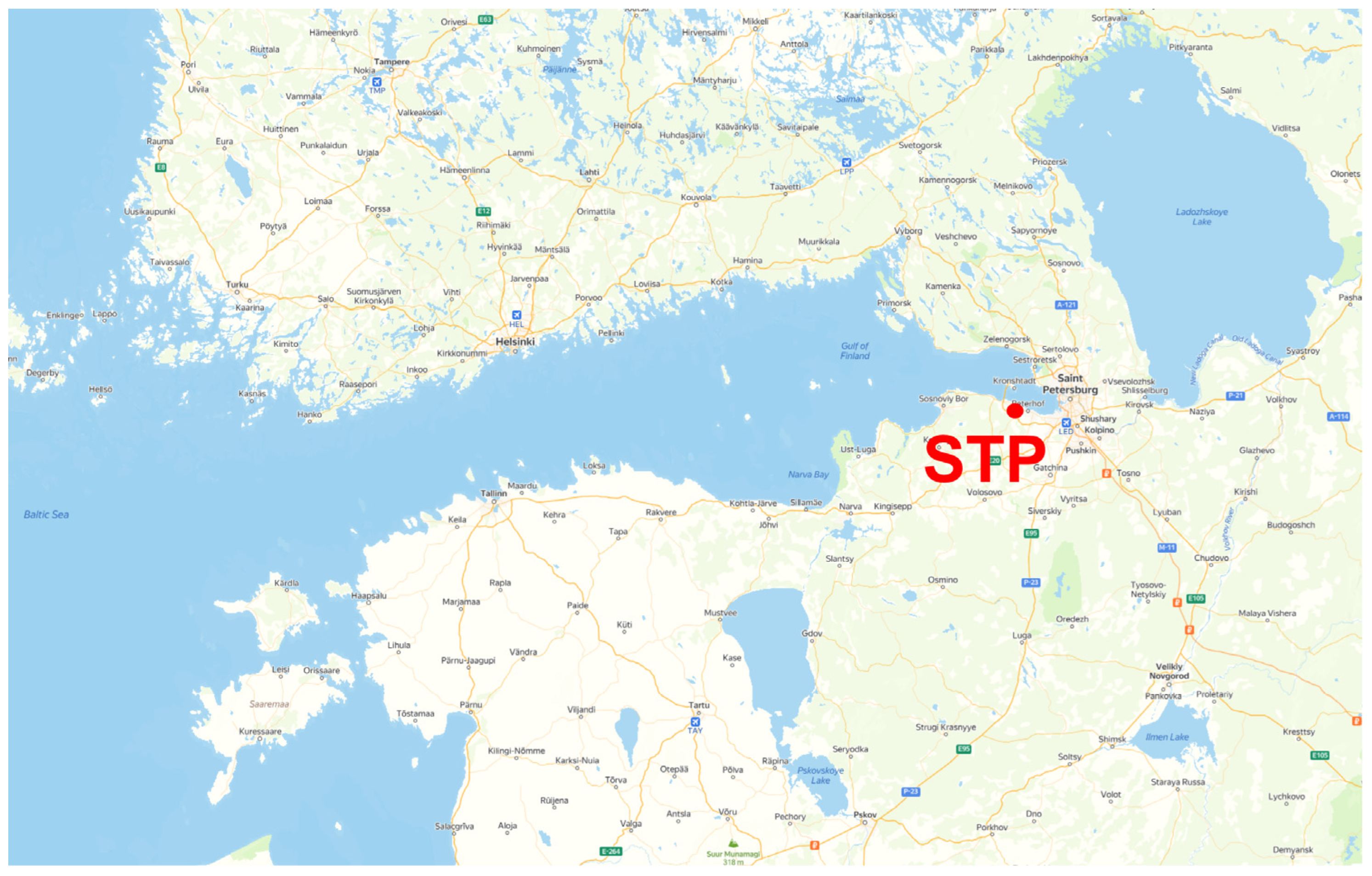
Section 1: general information on the SPbU atmospheric monitoring station including geographical, climate and weather features;

-

Section 2: a description of the FTIR system installed at the STP station, and an overview of the inverse methods and retrieval strategies used to derive the total columns/profiles of the target gases;

-

Section 3: Results and Discussion, including the characterization of the retrieval results and a time series analysis aimed at identifying long-term trends for LLGHG total columns;

-

Conclusions.

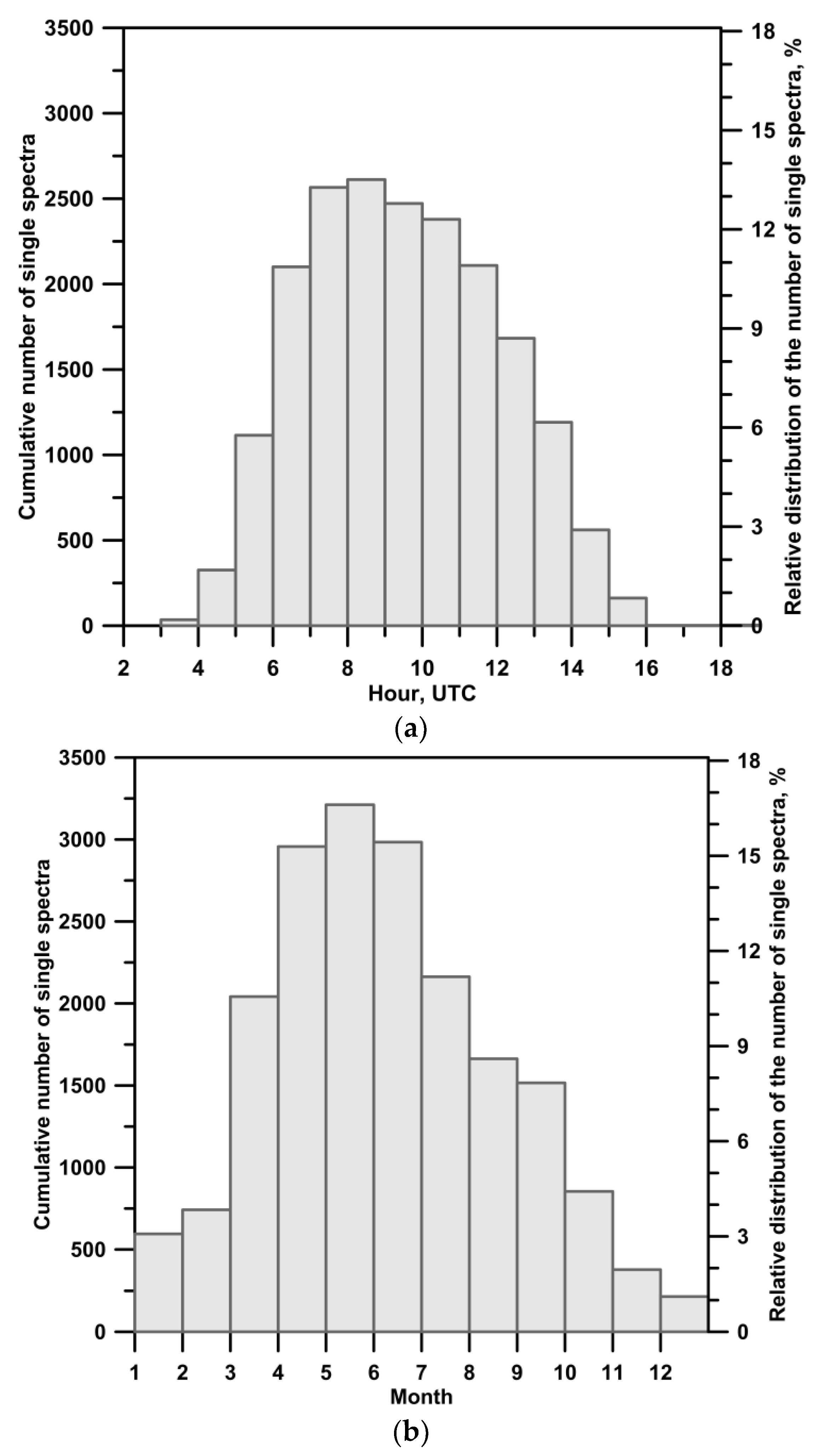
General Information about the SPbU Atmospheric Monitoring Station

The atmospheric monitoring station of SPbU is a mid-latitude observational station located at 59.88°N, 29.83°E, 20 m asl. It was established in the 1970s (https://phys.spbu.ru/englishpages/history.html, accessed on 23 March 2024) by the efforts of Saint Petersburg State University (former Leningrad State University). In 2016, the atmospheric monitoring station of SPbU joined the NDACC network [20] as the St. Petersburg site (https://www.ndaccdemo.org/stations/st-petersburg-russian-federation, accessed on 23 March 2024). The instruments for atmospheric monitoring are installed in the suburban Peterhof campus of SPbU, which is located at a distance of ~35 km southwest from the center of St. Petersburg. The geographic location of the observational site of SPbU is indicated on the map in Figure 1.

St. Petersburg is the second largest city in Russia and the fourth largest city in Europe. According to the official information, the population of St. Petersburg reached ~5.6 million in 2023 (http://council.gov.ru/en/structure/regions/SPE/, accessed on 23 March 2024). The climate of St. Petersburg and its suburbs is classified as humid continental (Dfb—Köppen climate classification) with moderately mild winters and moderately warm summers (http://www.pogodaiklimat.ru/climate/26063.htm, accessed on 23 March 2024, in Russian). The air masses coming from the Atlantic have the greatest influence on the climate of the region. Highly variable weather, with the frequent changes of Polar and Arctic air masses, is largely defined by cyclonic activity. On average, the winds of the western, north-western and south-western directions represent almost 46% (in autumn—about 50%) of all winds. Due to the predominance of westerly winds, most of the observations at the monitoring station are performed outside the St. Petersburg pollution plume and represent a regional background. In addition to FTIR observations, cases of air pollution from both anthropogenic and natural emissions [21] can be detected at the STP station using the NO₂ DOAS measurements [22] as well as in situ monitoring of NO_X, O₃, CO, CH₄ and CO₂ concentrations in the ambient air [23,24,25]. Mostly, these observational facilities are provided and maintained by the GEOMODEL Resource Center of the SPbU Research Park (https://researchpark.spbu.ru/en/geomodel-eng, accessed on 23 March 2024).

2. Instruments and Methods

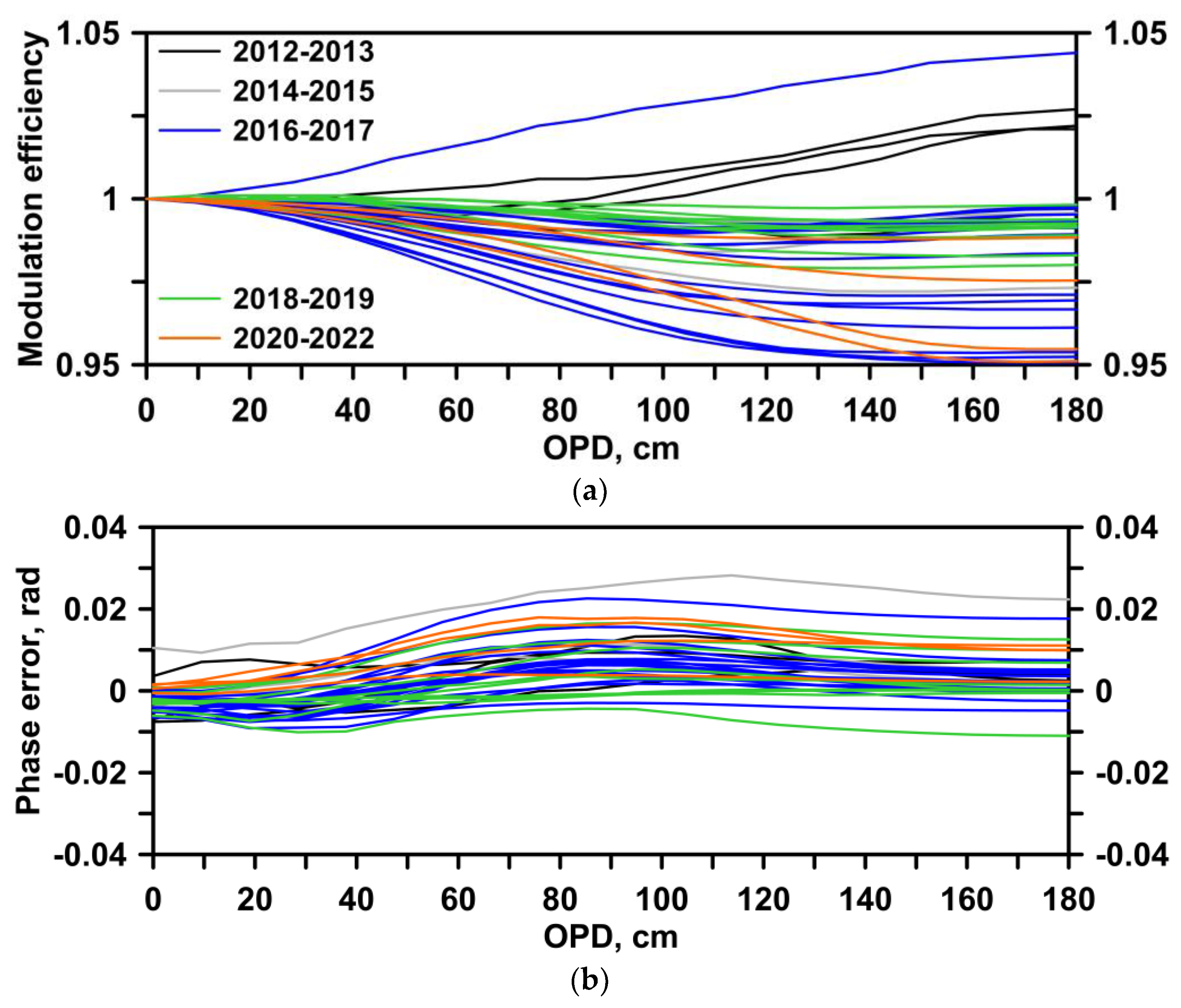
2.1. SPbU FTIR System

In January 2009, ground-based Fourier-transform infrared observations of direct solar radiation in the mid infrared (MIR) spectral region had been started in testing mode at the St. Petersburg site (SPbU). Routine FTIR measurements were launched in March 2009. In 2016, the FTIR system operated by the Atmospheric Physics Department was certified as an IRWG (the Infrared Working Group) NDACC instrument (https://www.ndaccdemo.org/stations/st-petersburg-russian-federation, accessed on 23 March 2024).

The high spectral resolution FTIR system [26,27] replaced the low resolution (~0.4–0.6 cm⁻¹) solar IR dispersive (grating) spectrometer used at the St. Petersburg site in 1991–2009 for total column (TC) measurements of CH₄ and CO [28,29].

The FTIR system is installed in the building of the Faculty of Physics of SPbU. It consists of a commercial Bruker IFS 125HR Fourier transform spectrometer (FTS) with a maximum spectral resolution Δν = 0.0019 cm⁻¹ and a self-designed solar tracker developed and assembled at the Atmospheric Physics Department of SPbU [30]. The FTS and precise positioning sensor of solar tracker are placed in an air-conditioned room. The Bruker IFS 125HR is equipped with LN-cooled InSb and MCT detectors. For routine atmospheric measurements, we use three broadband optical filters (F1, F2, and F3) with the following transmittance bands: 2350–5400 cm⁻¹ (in combination with InSb detector), 1700–3400 cm⁻¹ (in combination with InSb detector), and 650–1400 cm⁻¹ (in combination with MCT detector).

The routine monitoring of FTS alignment is performed using the laboratory spectra of a HBr cell (#61) and N₂O cell (#3). Since the first HBr spectrum measurement in April 2012, we controlled the state of IFS 125HR approximately once a month. The modulation efficiency and phase error affecting the instrumental line shape were retrieved from cell spectra using LINEFIT v.14.5 software [31]. These values obtained using HBr cell during 2012–2022 are given in Figure 2a,b.

In total, within the period of 2009–2022, FTIR observations at the St. Petersburg site have been performed for 1045 days (~19,300 single spectra), i.e., ~80 days per year on average. Between 2009 and 2022, there were four gaps in the FTIR data due to FTS and solar tracker failures and their subsequent troubleshooting.

Atmospheric FTIR observations use the sun as a light source, and therefore these types of remote measurements are performed under clear sky conditions or when the cloud cover has gaps sufficient to record at least a single spectrum. The distribution of measurement days over a year is uneven for St. Petersburg, due to high cyclonic activity in autumn and winter, and also due to the significant seasonal dependence of diurnal solar illumination: from 5 h 51 min (winter solstice) to 18 h 50 min (summer solstice). On the 22nd of December the value of the SZA (sun zenith angle) is larger than 83.50° during the whole day. Diurnal, seasonal and inter-annual cumulative distributions of the number of single spectra acquired using all three optical filters (F1, F2, and F3) are given in Figure 3a, Figure 3b and Figure 3c, respectively.

The typical configuration of the FTIR system, which is used for the GHG monitoring in the MIR spectral region at the STP station, is given in

Table 2. Typical FTIR system setup for MIR atmospheric measurements of GHG at the St. Petersburg station.

Detector	LN-Cooled InSb
Beamsplitter	KBr
Fieldstop, mm	0.8–1.3
Δν, cm−1 (OPD, cm)	0.005 (180)
Registered spectral range, cm−1	1700–3400 (optical filter F2)
Number of scans	4–10

. An example of solar spectra recorded at the St. Petersburg site is presented in Figure 4.

2.2. Inverse Methods and Retrieval Strategies

If we consider the ground-based FTIR observations, a solution of an inverse problem implies deriving quantitative information on total columns (TCs) and/or the volume mixing ratio (VMR) vertical profiles of target gases in the atmosphere from the MIR spectra of solar radiation. From a physical point of view, the retrieval of a gas VMR profile is possible due to the dependence of the spectral line shapes of the gas molecules on the vertical profiles of temperature and pressure in the atmosphere. The formalism for solving such an ill-posed problem of atmospheric sounding, which requires a certain amount of a priori information, has been developed by Tikhonov [32] and Rodgers [33,34]. Optimal Estimation (OE) and Tikhonov–Phillips regularization (T–P) are the two most common algorithms implemented in the retrieval codes SFIT (https://wiki.ucar.edu/display/sfit4/, accessed on 23 March 2024) [35,36] and PROFFIT [37,38]. Both codes are used by IRWG NDACC groups for the FTIR spectra processing. The details on the theory of inverse techniques and practical application to the ground-based FTIR observations can be found in the papers by Tikhonov [32], Rodgers [34], Pougatchev et al. [35], Rinsland et al. [36], Hase et al. [37], Sussmann et al. [39], and García et al. [40]. T–P L1 regularization [41] is used in the TC/VMR retrievals in the cases where the covariance matrix S_a, which is a critical point for OE, cannot be constructed using reliable independent observations [42].

The TCs and VMR profiles of atmospheric CH₄, N₂O, CO, HCN, C₂H₆, HCl, HF, O₃, HNO₃, and ClONO₂ are routinely measured at the St. Petersburg site. Corresponding retrieval results for all these trace gases are available at the NDACC database (https://www-air.larc.nasa.gov/missions/ndacc/data.html, accessed on 23 March 2024) in the form of HDF files. In addition to the above-mentioned NDACC mandatory list of species, the following gases are measured at the STP site: CO₂, H₂O, CFC-11, CFC-12, HCFC-22, H₂CO, CH₃OH, HCOOH, C₂H₂, OCS, NH₃, NO₂ and N₂. Data on CFC-11, CFC-12, HCFC-22, H₂CO, OCS can also be found at NDACC database, and the information on other gases can be provided upon request. In the current work we are focusing on the FTIR monitoring of long-lived greenhouse gases (CH₄, N₂O, and CO₂). All the retrievals of these species have been conducted by SFIT4 tools (v. 4.09.4.4).

For the greenhouse gases from the IRWG mandatory list (i.e., CH₄, N₂O), the retrieval of TCs and VMR profiles from high resolution FTIR spectra acquired at the STP site is mainly based on the IRWG Uniform Retrieval Guidelines [43]. This document contains the recommended retrieval strategies, which can be used by most of the FTIR sites with various geographical, climate and weather conditions. For CO₂, we use retrieval strategies which were recently developed by the IRWG community (for details, please, see [44]).

The a priori information, which is homogeneous for all IRWG observational sites, was constructed for most of the trace gases using WACCM v.6 simulations (Whole Atmosphere Community Climate Model, https://ncar.ucar.edu/what-we-offer/models/whole-atmosphere-community-climate-model-waccm, accessed on 23 March 2024) [45]. It includes:

-

site-specific a priori VMR profiles of the retrieved and interfering species;

-

site-specific a priori covariance matrixes (S_a) for the retrieved and interfering species (constructed using WACCM v.6 data on variability of VMR profiles).

In our retrievals, all priori information is not time-dependent, i.e., we set it once and keep it unchanged when processing all the years of measurements (2009–2022), so the detected temporal variations of the target gases are completely based on observations.

A homogeneous input information on atmospheric pressure and temperature profiles, which is necessary for the forward model calculations, is provided by NOAA/NWS/National Centers for Environmental Prediction (NCEP) in the form of daily (at 12:00 UTC) profiles of temperature and geopotential heights on 18 pressure levels from 1000 to 0.4 hPa at NDACC stations (https://www-air.larc.nasa.gov/missions/ndacc/data.html?NCE12.00UTCP=ncep-list, accessed on 23 March 2024). Spectroscopy linelists are critical input data for getting reliable retrieval results. HITRAN databases [46,47,48,49] and ATM linelists created by G. Toon [50] (NASA Jet Propulsion Laboratory, http://mark4sun.jpl.nasa.gov/toon/linelist/linelist.html, accessed on 23 March 2024) were mainly used for this purpose. For each target gas we provided information on spectroscopy linelists in the third column of

Table 3. Overview of retrieval strategies used at the STP FTIR site. Species from the IRWG mandatory list are marked by asterisk (*). The designation “L1” in the fifth column denotes the first-order Tikhonov–Phillips constraint.

Target Gas	Spectral Intervals, cm−1	Spectroscopic Linelist	Retrieved Interfering Gases	Regularization Type	References
CH4 *	2613.70–2615.40 2835.50–2835.80 2921.00–2921.60	HITRAN 2000 (with 2001 updates)	HDO, H2O, CO2, NO2	T–P L1	[39,43]
CO2	2620.55–2621.10 2626.40–2626.85 2627.10–2627.60 2629.275–2629.950	HITRAN 2008, HITRAN 2009 for H2O	H2O, HDO, CH4	T–P L1	[44]
N2O *	2481.30–2482.60 2526.40–2528.20 2537.85–2538.80 2540.10–2540.70	HITRAN 2008	CO2, H2O, CH4, O3	T–P L1	[43]

. Information about solar spectral lines according to [51] is incorporated into SFIT4 processing tools.

3. Results and Discussion

3.1. Characterizing Retrieval Results: Spectral Fitting, Uncertainty Analysis and Averaging Kernels

To describe retrieval results, the following main characteristics are usually reported (the examples can be found in the papers [42,44,52,53,54]:

-

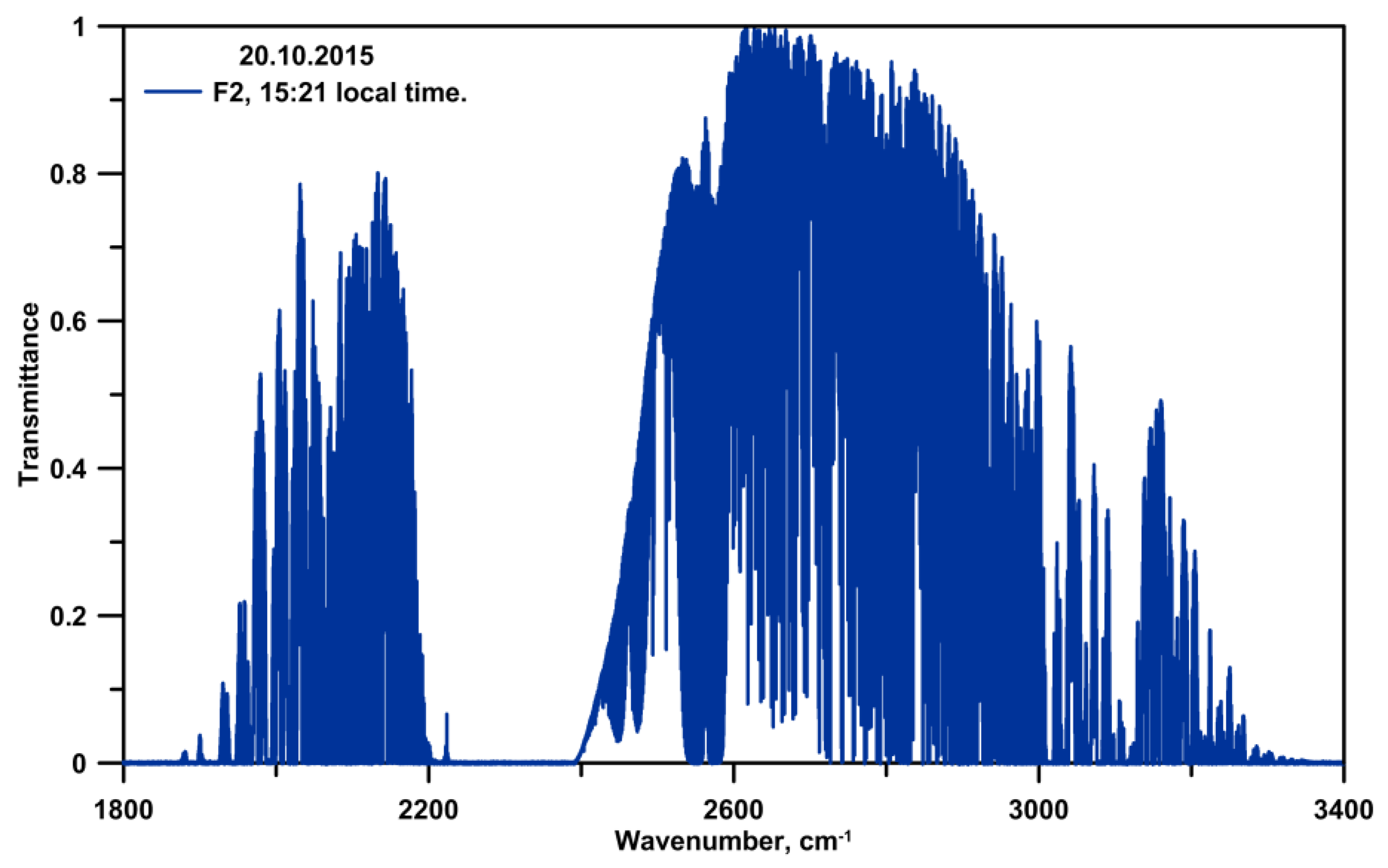
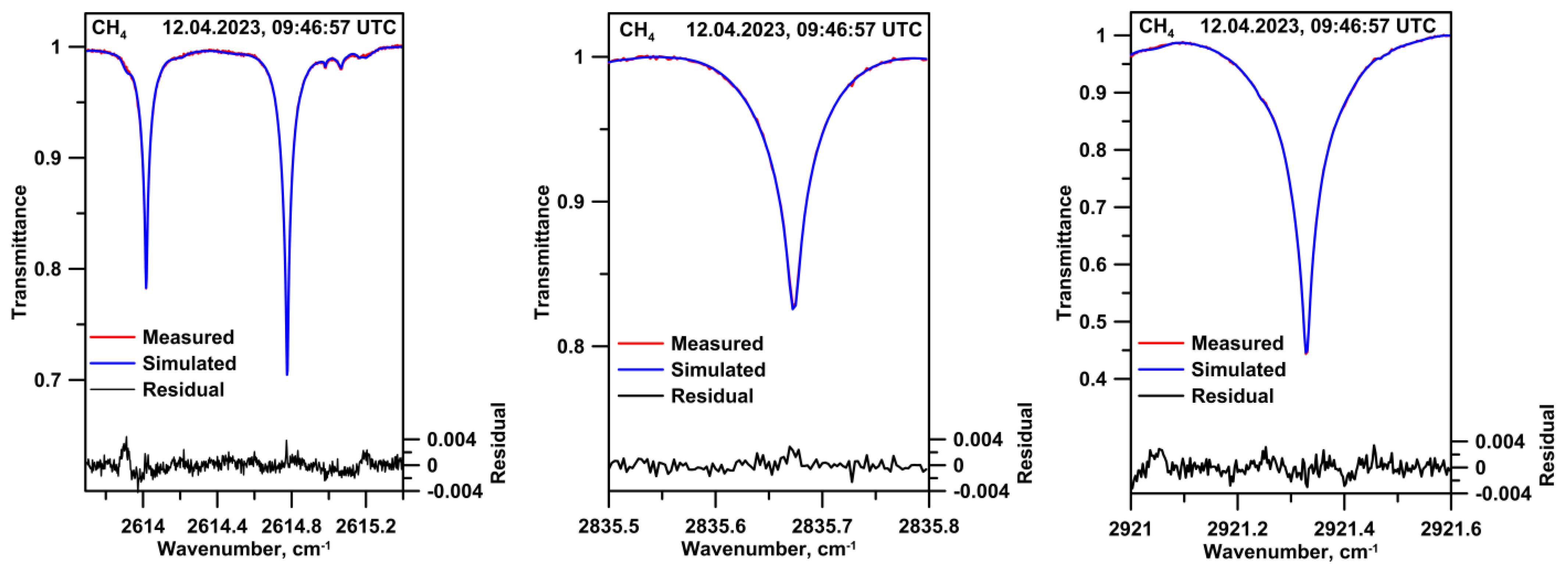
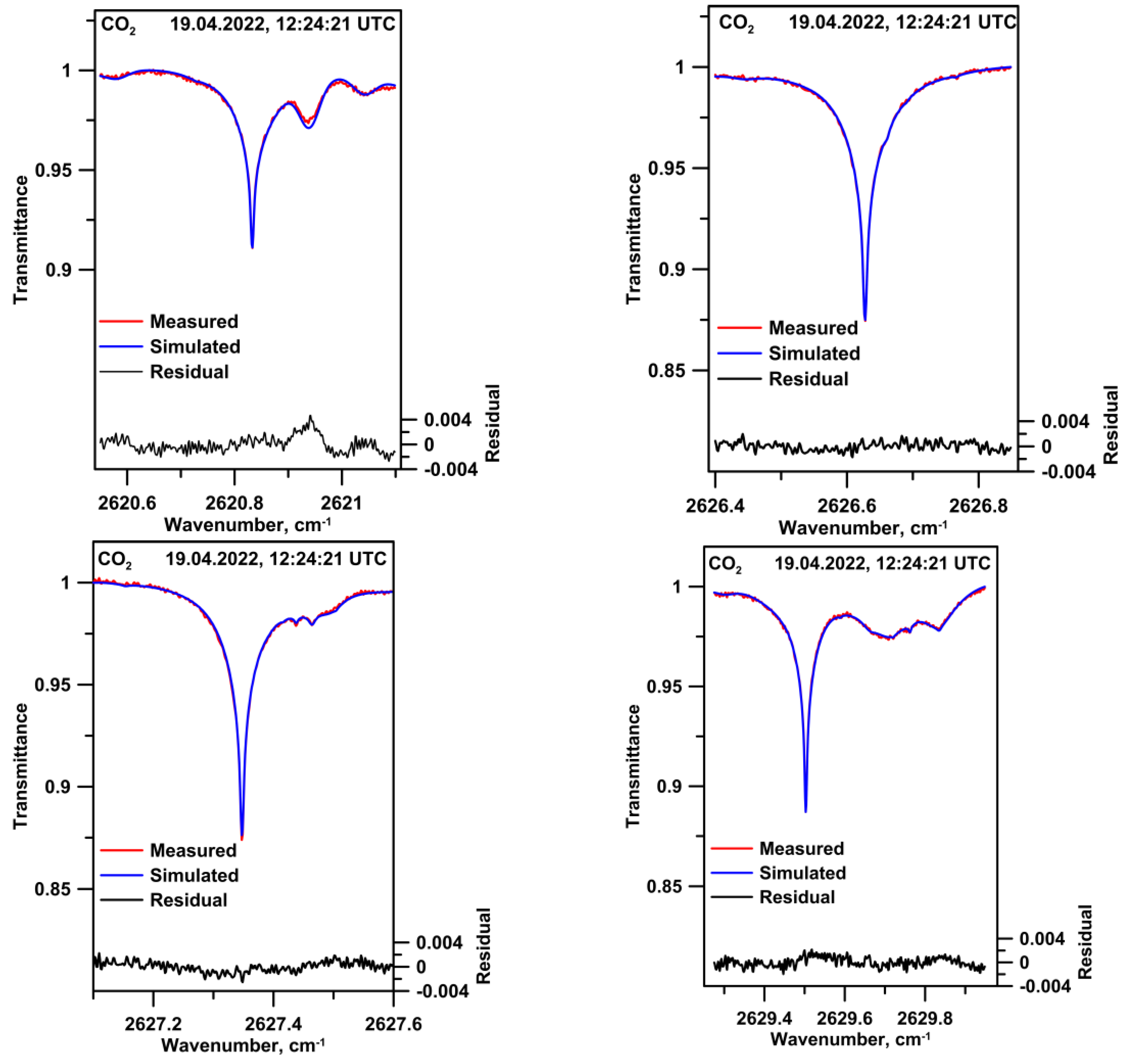
the RMS discrepancy between the observed and simulated spectra as a measure of the quality of spectral fitting (see column 3 of

Table 4. Mean values (M) and standard deviations (σ) of TC, X_GAS, DOFS (“total”—for the entire atmospheric column, and “tropo”—for the troposphere), and also random, systematic, and smoothing uncertainties. All values were obtained as a result of FTIR spectra processing within the period 2009–2022.

Target Gas	TC, molec/cm2	XGAS, ppm	RMS, %	DOFS		Random Uncertainty, %	Systematic Uncertainty, %	Smoothing Uncertainty, %
				Total	Tropo
	M ± σ	M ± σ	M ± σ	M ± σ	M ± σ	M ± σ	M ± σ	M ± σ
CH4	(3.885 ± 0.089) × 1019	1.807 ± 0.038	0.14 ± 0.03	2.5 ± 0.3	1.3 ± 0.2	1.5 ± 0.9	3.6 ± 0.1	0.5 ± 0.1
CO2	(8.79 ± 0.23) × 1021	409 ± 10	0.14 ± 0.03	1.4 ± 0.2	0.7 ± 0.1	2.2 ± 0.9	3.4 ± 0.2	0.5 ± 0.4
N2O	(6.59 ± 0.12) × 1018	0.3071 ± 0.0055	0.18 ± 0.06	2.6 ± 0.2	1.6 ± 0.1	1.2 ± 0.2	2.6 ± 0.1	0.2 ± 0.1

). The typical examples of spectral fitting for corresponding spectral intervals used in the CH₄, CO₂, and N₂O retrievals are given in Figure 5, Figure 6 and Figure 7, respectively;

-

the uncertainty (error) budget including the analysis of random, systematic, and smoothing uncertainties (see columns 7–9 of Table 4);

-

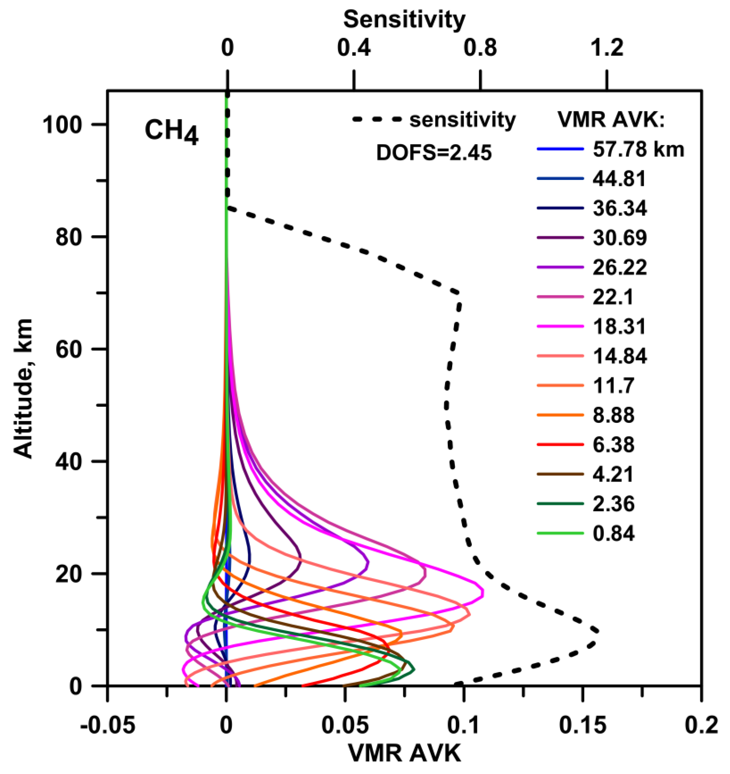
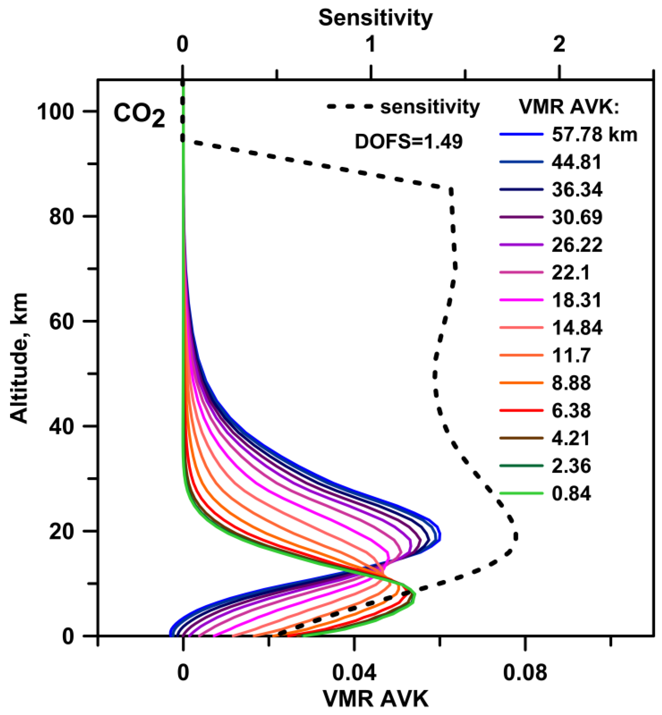
the averaging kernels (AVKs) for VMR, the “sensitivity” of the retrievals to the measurements [55] (Figure 8, Figure 9 and Figure 10), and the value of degrees of freedom for the signal (DOFS; see columns 5–6 of Table 4), which characterize the vertical sensitivity of the retrieval. The sensitivity at altitude level i is calculated as the sum of the elements of the corresponding averaging kernel Σ_kAVK_ik;

-

retrieved total columns (TCs), column-averaged dry-air mole fraction (X_GAS) (see columns 2–3 of Table 4). We calculated X_GAS by dividing the total column of a target gas (TC_GAS) by the dry pressure column (DPC) parameter [44,56]:

$$X_{GAS}=\frac{T{C}_{GAS}}{DPC}$$

(1)

$$DPC=0.2095\frac{P_S}{g(\phi )m_{dryair}}-T{C}_{H2O}\frac{m_{H2O}}{m_{dryair}}$$

(2)

where m_dryair—the molecular mass of dry air (28.964 g mol⁻¹);

m_H2O—molecular mass of H₂O (18.02 g mol⁻¹);

P_s—surface pressure (mb), which is taken from NCEP input data used in the retrievals;

g(φ)—the latitude-dependent gravitational acceleration;

TC_H2O—the total column of water vapor, which is a result of separate retrieval of H₂O TC.

Table 4 contains information about the mean (M) values of TC, X_GAS, RMS, DOFS, systematic, random, and smoothing uncertainties averaged over the entire measurement period (2009–2022); standard deviation (σ) is given as a measure of the variability of the reported values.

The “AVK for VMR” functions and the “sensitivity for TC” functions have gas-specific altitude dependence (Figure 8, Figure 9 and Figure 10). Together with the DOFS value (which is equal to the trace of AVK matrix), they characterize the vertical sensitivity of FTIR observations to the abundance of a target gas. AVKs characterize the degree of smoothing of the true profile in the retrieval procedure; the sensitivity at each altitude indicates the fraction which comes to the retrieval from the measurement rather than from the a priori information. The DOFS value (a number of independent pieces of information) can be interpreted in our case as a number of atmospheric layers for target gas which can be retrieved independently from observations. For DOFS, we show two values in Table 4: the value of DOFS for the entire atmospheric column and the value of DOFS which was calculated separately for the troposphere (0–10 km). So, according to Table 4, only the TC value can be obtained in the case of the CO₂ retrieval, since the corresponding DOFS < 2.0 (i.e., we have an independent piece of information on only one atmospheric layer). Columns in two atmospheric layers can be obtained in the cases of the CH₄ and N₂O retrieval: in the troposphere where DOFS > 1.0 and in the remaining overlying atmosphere (10–106 km).

The quantitative evaluation of uncertainties based on the formula developed by Rodgers [33,34] is incorporated into the SFIT4 retrieval tools. This ensures the homogeneity of error estimates obtained by different IRWG groups. The error budget for all target species is given in Table 4, and it consists of the following components:

-

the systematic error which originates from the systematic uncertainties of the following forward model/input parameters: spectroscopy (line intensity, line broadening by pressure and temperature, solar line intensity), sun zenith angle (SZA), curvature of the spectrum baseline, phase, optical path difference (OPD), field of view (FOV). The systematic error budget is mainly defined by uncertainties in the spectroscopic information, i.e., line intensities and broadening factors [40];

-

random error, which includes measurement error (due to measurement noise), random uncertainties of forward model/input parameters, uncertainties of the parameters of the retrieval algorithm, interference error (due to retrieved interfering gases) and smoothing error. The dominant inputs into random uncertainty are as follows: measurement noise, baseline uncertainty, and uncertainties in the input temperature profile [40,42];

-

the smoothing error, which is assumed to be random in our study (with no systematic component), reflects the uncertainty due to the limited vertical resolution of the FTIR observations.

The average values of random and systematic uncertainties, as well as smoothing errors estimated for all three gases on the bases of the results of the fourteen-year retrievals at the STP site are of 1–2%, 3–4% and less than 0.5%, respectively (see Table 4, columns 7–9).

3.2. Time Series Analysis: Long-Term Trends of GHG TCs

Figure 11, Figure 12 and Figure 13 display CH₄, CO₂, and N₂O TC and X_GAS time series for 2009–2022 as measured at the STP FTIR station. Previously, data filtering was carried out. Measurements with high RMS/DOFS values [39] which were beyond the average value of RMS/DOFS plus 3σ were rejected. In addition to the RMS/DOFS criterion, the outliers that manifested in obviously inadequate (extremely low or extremely high beyond the 3σ variability limits) values of the LLGHG TCs were also excluded from the time series. Before filtering, the LLGHG time series included 6278 single measurements each. After applying the above mentioned criteria, the number of single measurements for CH₄, CO₂ and N₂O became 6168, 6103 and 6163, respectively.

We assumed that the analyzed time series of TC can be approximated by a model function F_TC(t) that is the sum of a linear function and a set of N harmonic functions:

$$F_{TC}\left(t\right)=a+b\cdot t+{\displaystyle \sum _{i=1}^N{c}_i}cos\left({\alpha }_{i}t+{\phi }_i\right)$$

(3)

where t is time; and a, b, c_i, α_i and φ_i are the coefficients to be determined.

This is a typical approach which is widely used for the analysis of time series of atmospheric trace gases [54]. The TC long-term trend is equal to the coefficient b, which determines the slope of the linear function (see Equation (3)). To obtain statistical characteristics (the mean value of b, the confidence intervals/uncertainty of b) of long-term trends for CH₄, CO₂ and N₂O, the analysis of TC time series of target gases was carried out in the following three steps:

• Harmonic analysis of the time series of LLGHG TCs. For this purpose, time series were previously detrended using the simple linear regression. After detrending, the Lomb–Scargle method, which is a modification of Fourier analysis for uneven time series, was applied [57,58,59]. The outcome is a set of n periods/frequencies having peaks (maxima) of spectral density in periodogram.
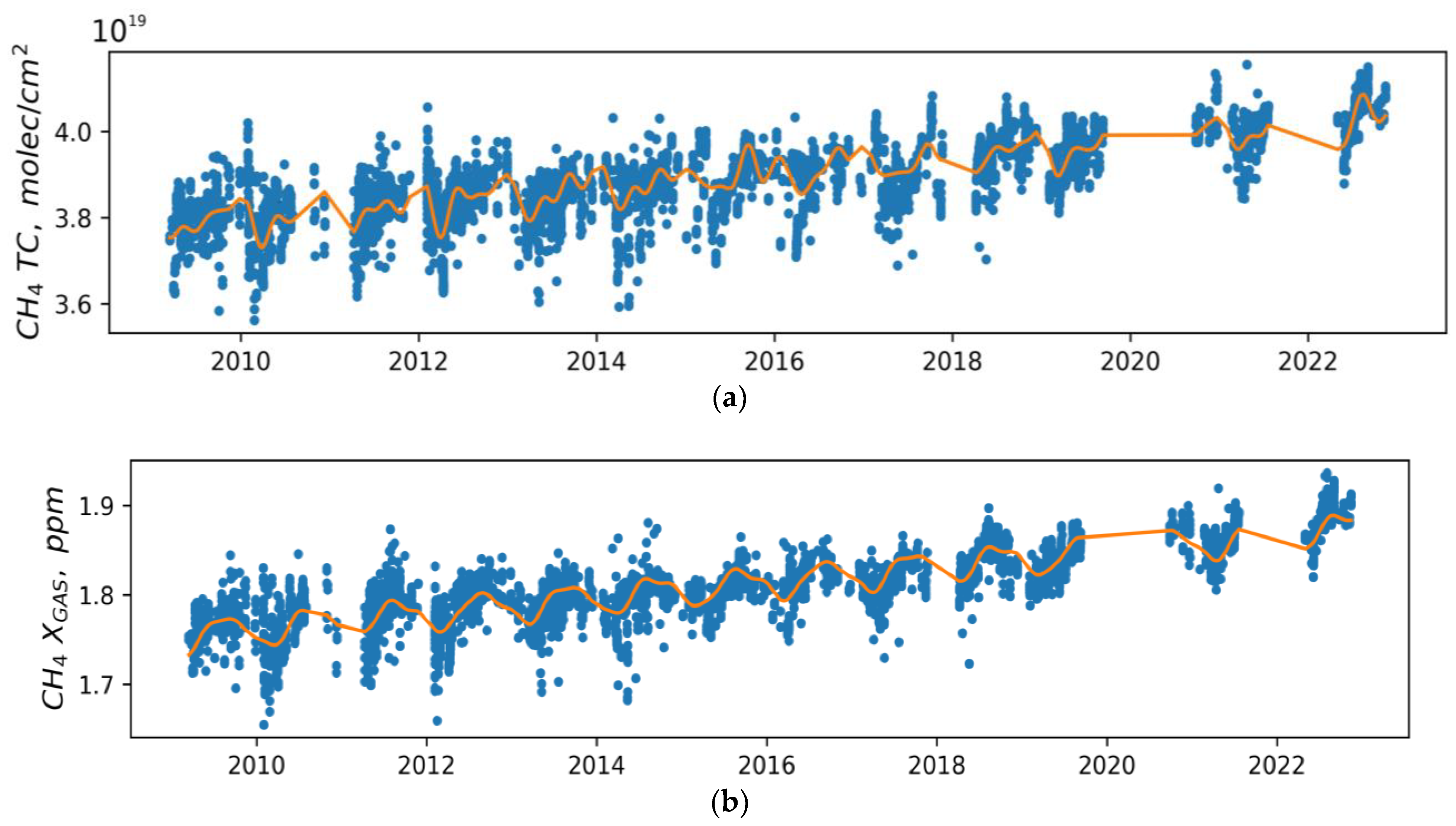
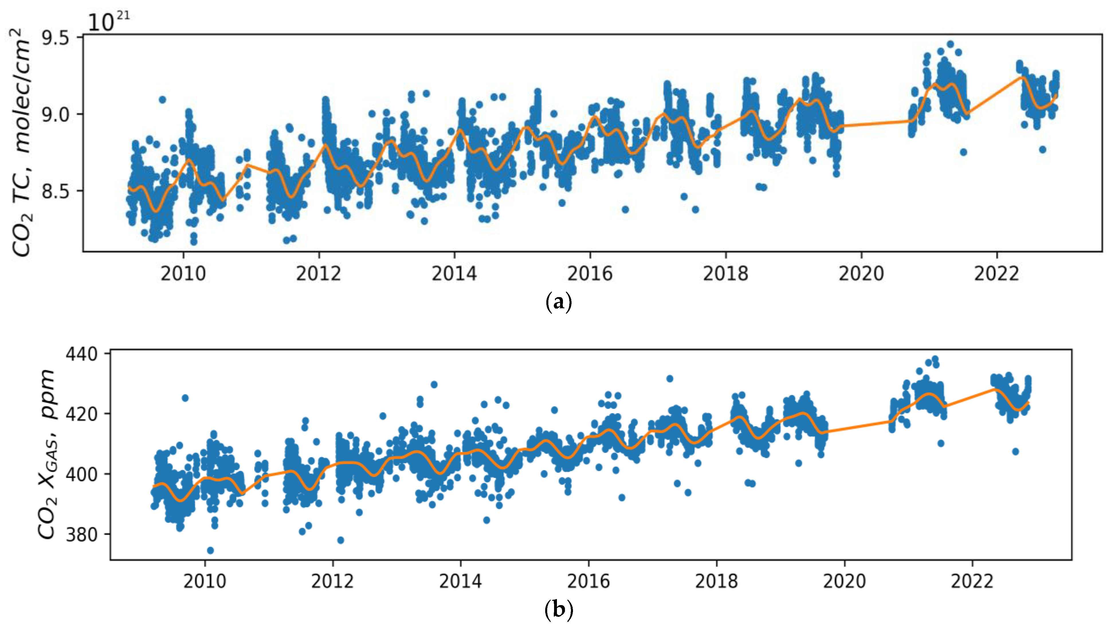
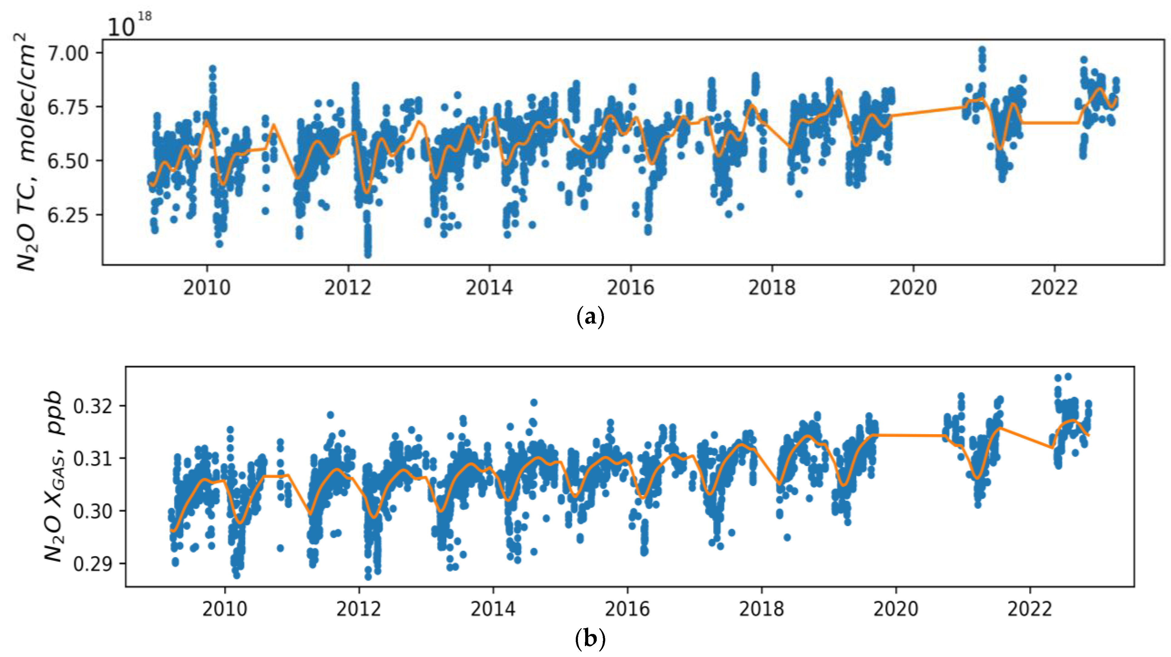
• Estimation of an optimal set of N harmonic functions (from the whole set n) which provides the best approximation. To achieve this goal, we evaluated the performance of a model F_TC(t) on unseen data (cross-validation technique). It involves dividing the available time series (TC) into multiple subsets, using one of these subsets as a validation set, and training the model on the remaining subsets (https://www.geeksforgeeks.org/cross-validation-machine-learning/, accessed on 23 March 2024). We made this analysis multiple times, including i most significant harmonic functions at each step (starting from i = 1 and ending with i = n). For each step we determined the RMS value of the discrepancy between validation set and model function F_TC(t). The optimal number N provides the minimum value of the RMS discrepancy between the model and the validation set. Approximations F_TC(t) for 2009–2022, which were constructed with the optimal numbers N, are presented in Figure 11, Figure 12 and Figure 13 by solid lines.
• Evaluation of the mean value of a trend (coefficient b) and its confidence intervals/uncertainty. For this purpose, the bootstrapping approach was implemented [54,60]. To characterize the distribution function for trend (allowing us to estimate the mean slope b and 1σ uncertainty as distribution halfwidth), we used a bootstrap population of ~400 (a further increase of this number does not lead to any noticeable changes in the results).

At all stages, data fitting was performed by the least squares method. The X_GAS trends were determined in the same three-step way as for TC.

Table 5 presents the estimates of the coefficient b (slope) which characterize the long-term trends of LLGHGs’ TCs and X_GAS in the atmosphere for different periods of time. The second column of this table shows the mean values of the long-term trends of target gases with 95% confidence intervals (2σ) for the fourteen-year (2009–2022) period of FTIR measurements at the STP station observations. The third column (with subcolumns) presents the results for the eleven-year (2009–2019) observations. If the variability of TC is influenced by atmospheric pressure at the observational site, then the transition from the TC to the X_GAS excludes the influence of atmospheric pressure variations (see Equation (2)). X_GAS is a value widely used in studies of the atmospheric gaseous composition; however, in our opinion, the long-term processes affecting the GHGs content in the atmospheric column can be better characterized by the TC trend rather than the X_GAS trend. If we take into account possible (hypothetic) trends in atmospheric pressure, we can conclude that the TC trend characterizes an increase of the total number of molecules absorbing IR radiation in the column of the atmosphere.

Reasonable agreement of CH₄ and N₂O TC trends for 2009–2019 captured by FTIR measurements at the STP site of SPbU, Izaña Observatory (IO, 28.3°N, 16.5°W, ~2370 m a.s.l.) [40], and the University of Toronto Atmospheric Observatory (TAO, 43.66°N, 79.40°W, 174 m a.s.l.) [61] can be seen if we compare the third, the fourth, and the fifth columns of Table 5. Here we should note that STP, IO and TAO are members of the NDACC network; therefore, FTIR observations and their processing are consistent in general for all three sites.

The above-described data analysis algorithm was also applied to the TC time series of CH₄, CO₂, and N₂O simulated by the ECHAM/MESSy Atmospheric Chemistry (EMAC) model (2009–2019). The EMAC model is a numerical chemistry and climate simulation system which includes sub-models describing the processes in the troposphere and in the middle atmosphere and their interaction with oceans, land and anthropogenic impacts [62,63]. The simulation includes a comprehensive atmospheric chemistry setup for the troposphere, the stratosphere and the lower mesosphere. The EMAC model profiles of trace gas concentrations, pressure and temperature were simulated directly for the geographical location of the STP site. For an accurate comparison of the model (EMAC) and the experimental (FTIR) trends, an EMAC simulation of the FTIR time series (EMAC TC_{FTIR_AVK}) was created. For this purpose, we generated a set of model profiles for the dates coinciding with the dates of FTIR measurements, after that, following the Rodgers and Connor [64] formula (see Equation (4)), model profiles were convolved (smoothed) with the AVKs of corresponding FTIR measurements as follows:

$$x_s=A{(\mathrm{x} - \mathrm{x}}_a)+{\mathrm{x}}_a$$

(4)

where x is the EMAC profile of a target gas; x_s is the smoothed EMAC profile of a target gas; A is the FTIR AVK matrix; x_a is the FTIR a priori profile of target gas.

Finally, smoothed EMAC profiles (x_s) were used for the calculation of total columns (EMAC TC_{FTIR_AVK}). Trend estimations for EMAC TC_{FTIR_AVK} of LLGHGs are given in the sixth column of Table 5. It can be seen that the trends of TC obtained from the FTIR monitoring results and from model simulations for N₂O and CO₂ agree within 3σ. The largest difference in the TC trends, amounting to 0.28% yr⁻¹ and exceeding the 3σ limit, was obtained for CH₄.

Table 5. The LLGHGs linear trends (±2σ) in the atmosphere revealed from the results of FTIR measurements at the STP site in comparison to IO [40] and TAO [61] trends, EMAC model trends, global VMR trends obtained at the GAW in situ observational network for GHGs (WMO, 2022), and VMR trends determined using in situ observations of CH₄ and CO₂ at STP site [65]. The periods for which LLGHGs trends were estimated are given in the second row of the table.

Target Gas	Mean Trend
	2009–2022	2009–2019				2012–2021		2013–2019
	FTIR TC, FTIR XGAS	FTIR TC	FTIR TC (IO)	FTIR TC (TAO)	EMAC TCFTIR_AVK	FTIR XGAS	Global In Situ VMR (GAW)	FTIR XGAS	In Situ VMR
CH4, % yr−1 ppb yr−1	0.46 ± 0.02 8.8 ± 0.4	0.44 ± 0.04	0.43 ± 0.03	0.41 ± 0.03	0.16 ± 0.04	0.47 ± 0.05 8.5 ± 1.0	0.51 9.2	0.52 ± 0.04 9.4 ± 0.7	0.49 8.6 ± 0.8
CO2, % yr−1 ppm yr−1	0.56 ± 0.01, 2.28 ± 0.05	0.58 ± 0.02	-	-	0.52 ± 0.02	0.61 ± 0.02 2.52 ± 0.07	0.61 2.46	0.61 ± 0.04 2.5 ± 0.1	0.60 2.42 ± 0.1
N2O, % yr−1 ppb yr−1	0.28 ± 0.01 0.82 ± 0.03	0.26 ± 0.02	0.31 ± 0.03	-	0.20 ± 0.02	0.30 ± 0.03 0.91 ± 0.08	0.31 1.01	0.26 ± 0.04 0.8 ± 0.1	-

Table 5. The LLGHGs linear trends (±2σ) in the atmosphere revealed from the results of FTIR measurements at the STP site in comparison to IO [40] and TAO [61] trends, EMAC model trends, global VMR trends obtained at the GAW in situ observational network for GHGs (WMO, 2022), and VMR trends determined using in situ observations of CH₄ and CO₂ at STP site [65]. The periods for which LLGHGs trends were estimated are given in the second row of the table.

Target Gas	Mean Trend
	2009–2022	2009–2019				2012–2021		2013–2019
	FTIR TC, FTIR XGAS	FTIR TC	FTIR TC (IO)	FTIR TC (TAO)	EMAC TCFTIR_AVK	FTIR XGAS	Global In Situ VMR (GAW)	FTIR XGAS	In Situ VMR
CH4, % yr−1 ppb yr−1	0.46 ± 0.02 8.8 ± 0.4	0.44 ± 0.04	0.43 ± 0.03	0.41 ± 0.03	0.16 ± 0.04	0.47 ± 0.05 8.5 ± 1.0	0.51 9.2	0.52 ± 0.04 9.4 ± 0.7	0.49 8.6 ± 0.8
CO2, % yr−1 ppm yr−1	0.56 ± 0.01, 2.28 ± 0.05	0.58 ± 0.02	-	-	0.52 ± 0.02	0.61 ± 0.02 2.52 ± 0.07	0.61 2.46	0.61 ± 0.04 2.5 ± 0.1	0.60 2.42 ± 0.1
N2O, % yr−1 ppb yr−1	0.28 ± 0.01 0.82 ± 0.03	0.26 ± 0.02	0.31 ± 0.03	-	0.20 ± 0.02	0.30 ± 0.03 0.91 ± 0.08	0.31 1.01	0.26 ± 0.04 0.8 ± 0.1	-

The X_GAS trends for 2012–2021 estimated using FTIR measurements at the STP station and global VMR trends obtained at the GAW in situ observational network for GHGs [1] are presented in the seventh and eighth columns of Table 5. The ninth and tenth columns show the trends obtained using FTIR X_GAS data and the results of in situ monitoring of CO₂ and CH₄ VMR at the STP station in 2013–2019, respectively. It should be noted that the publication by Foka et al. [65] is devoted to the analysis of trends of in situ VMR measurements carried out at the same location where the FTIR observations were performed. A reasonable agreement (within 2σ) of the FTIR X_GAS trends with the in situ VMR trends reported in both papers [1,65] was obtained. When comparing trends of X_GAS with the results of the in situ monitoring of VMRs, it should be taken into account that, in contrast to the in situ measurements which characterize the lowest tropospheric layer (the surface layer), FTIR measurements characterize processes throughout the atmosphere with the maximum sensitivity corresponding to the middle and upper troposphere (see Figure 8, Figure 9 and Figure 10).

We would like to draw attention to the CO₂ TC trend over the fourteen-year period 2009–2022, which is equal to 0.56% yr⁻¹. This is the lowest trend value among the CO₂ TC trends reported in Table 5 for other shorter periods: 0.58% yr⁻¹ for 2009–2019; 0.61% yr⁻¹ for 2012–2021 and for 2013–2019. Our analysis has shown that the reason for this result was a significant drop in the growth rate of CO₂ in 2022, which was manifested not only in the CO₂ TC data obtained at the STP site, but also in the results of the in situ measurements. For example, at the high-altitude Mauna Loa observatory (~3400 m a.s.l.) where the VMR observations are representative for the free troposphere, the CO₂ annual mean growth rate in 2021 was (2.37 ± 0.11) ppm yr⁻¹, while in 2022 it dropped to (1.81 ± 0.11) ppm yr⁻¹ (the lowest value since 2008) [10,11].

It should be noted here that most NOAA GML stations are also part of the GAW WMO network. NOAA GML is the GAW WMO Central Calibration Laboratory (https://gml.noaa.gov/ccl/scales.html, accessed on 23 March 2024), responsible for maintaining and distributing the WMO Mole Fraction scale for GHGs concentrations in atmospheric air. It provides the compatibility of GHGs measurements on a global scale and ensures the consistency of the trends obtained using GAW WMO observations (given in Table 5) with the corresponding trends according to NOAA GML data, which we discuss below. A graphical comparison of the CH₄, CO₂ and N₂O X_GAS trends registered at the STP site over 2009–2022, with the global growth rates of VMR obtained for the same period by the NOAA Global Monitoring Laboratory (NOAA GML [10,66]), is shown in Figure 14a–c, respectively. This figure clearly demonstrates that for CH₄ and CO_2, the fourteen-year X_GAS trends (solid dark blue lines) lie within the 95% confidence limits (blue stripes in Figure 14a,b) of the mean global VMR growth rates (dashed light blue lines) obtained as a result of VMR in situ measurements carried out in 2009–2022 by the NOAA GML. In contrast to CH₄ and CO₂, the N₂O X_GAS trend lies inside the 99% confidence interval but outside the 95% confidence interval (blue shaded area in Figure 14c) of the mean global growth rates of the N₂O VMR.

4. Summary and Conclusions

In this paper, we provide a rigorous assessment of the trend parameters of the total columns of key atmospheric greenhouse gases derived from multi-year observations at our FTIR station. Over many years, we made extensive measurements of the CO₂, CH₄, and N₂O total columns using a high resolution FTS Bruker IFS 125HR at a midlatitude station located on the Baltic Sea coast.

We applied an original approach for the TC time series analysis, which combines the Lomb–Scargle method with the cross-validation and bootstrapping techniques. As a result, the fourteen-year trends of the CO₂, CH₄, and N₂O total columns for our FTIR site were evaluated. We carried out a comparison of our results with the trends obtained by the numerical modeling, and also by the in situ and FTIR atmospheric monitoring performed at different geographical locations.

The main findings of the paper are as follows:

• The retrieval strategies from IRWG NDACC for deriving the CO₂, CH₄ and N₂O total columns in the atmosphere from high-resolution FTIR spectra of direct solar radiation [39,43,44] have been adapted to the observational conditions at the STP station. The application of these adapted strategies resulted in the LLGHG TC retrievals with random and systematic uncertainties, on average, equal to 2.2% and 3.4% for CO₂, 1.5% and 3.6% for CH₄, 1.2% and 2.6% for N₂O, respectively. The average values of the smoothing uncertainty are of 0.5%, 0.5%, and 0.2% for CO₂, CH₄, and N₂O, respectively.
• The average values of the CO₂, CH₄, and N₂O TCs for 2009–2022 observed at the STP site constitute 8.79 × 10²¹ molec/cm², 3.885 × 10¹⁹ molec/cm² and 6.59 × 10¹⁸ molec/cm², respectively. The average values of X_GAS are equal to ~409 ppm for CO₂, ~1.807 ppm for CH₄, and ~0.3071 ppm for N₂O.
• An evaluation of the TC and X_GAS trends for LLGHGs was carried out using the combined approach for time series analysis. This approach included the Lomb–Scargle method for harmonic analysis, the least squares method for data fitting, the cross-validation algorithm to determine the optimal number of harmonic functions, and the bootstrapping technique to estimate the confidence intervals of trends. The fourteen-year (2009–2022) trends of TCs and X_GAS estimated using such a combined approach are as follows: (0.56 ± 0.01) % yr⁻¹ and (2.28 ± 0.05) ppm yr⁻¹ for CO₂; (0.46 ± 0.02) % yr⁻¹ and (8.8 ± 0.4) ppb yr⁻¹ for CH₄; (0.28 ± 0.01) % yr⁻¹ and (0.82 ± 0.03) ppb yr⁻¹ for N₂O;
• The TCs and X_GAS trends of LLGHGs observed at the STP site are in general agreement with the results of in situ VMR monitoring carried out at the same geographical location in the period 2013–2019 (Foka et al., in print), and with the independent estimates of global VMR growth rates obtained by the GAW network in the period 2012–2021 (WMO, 2022) and the NOAA Global Monitoring Laboratory in the period 2009–2022 [10,11,66]. There is reasonable agreement between the CH₄ and N₂O TC trends for 2009–2019 at the STP site, at Izaña Observatory [40], and also at the University of Toronto Atmospheric Observatory [61].
• A comparison of the EMAC model results with the FTIR data shows that for N₂O and CO₂, the EMAC and FTIR trends of TC agree within 3σ. The largest difference in the experimental and model TC trends, amounting to 0.28% yr⁻¹ and exceeding the 3σ limit, was obtained for CH₄.

References

1. WMO Greenhouse Gas Bulletin, No. 18, 26 October 2022, ISSN 2078-0796. Available online: https://library.wmo.int/idurl/4/58743 (accessed on 23 March 2024).
2. Montzka, S.A. The NOAA Annual Greenhouse Gas Index (AGGI). National Oceanic and Atmospheric Administration (NOAA) Earth System Research Laboratories Global Monitoring Laboratory. 2022. Available online: http://www.esrl.noaa.gov/gmd/aggi/aggi.html (accessed on 23 March 2024).
3. IPCC. Climate Change 2021: The Physical Science Basis. Contribution of Working Group I to the Sixth Assessment Report of the Intergovernmental Panel on Climate Change; Masson-Delmotte, V., Zhai, P., Pirani, A., Connors, S.L., Péan, C., Berger, S., Caud, N., Chen, Y., Goldfarb, L., Gomis, M.I., et al., Eds.; Cambridge University Press: Cambridge, UK; New York, NY, USA, 2021; 2391p. [Google Scholar]
4. Dlugokencky, E.J.; Houweling, S.; Bruhwiler, L.; Masarie, K.A.; Lang, P.M.; Miller, J.B.; Tans, P.P. Atmospheric methane levels off: Temporary pause or a new steady-state. Geophys. Res. Lett. 2003, 30, 1992. [Google Scholar] [CrossRef]
5. Kirschke, S.; Bousquet, P.; Ciais, P.; Saunois, M.; Canadell, J.G.; Dlugokencky, E.J.; Bergamaschi, P.; Bergmann, D.; Blake, D.R.; Bruhwiler, L.; et al. Three decades of global methane sources and sinks. Nat. Geosci. 2013, 6, 813–823. [Google Scholar] [CrossRef]
6. Prather, M.J.; Hsu, J.; DeLuca, N.M.; Jackman, C.H.; Oman, L.D.; Douglass, A.R.; Fleming, E.L.; Strahan, S.E.; Steenrod, S.D.; Søvde, O.A.; et al. Measuring and modeling the lifetime of nitrous oxide including its variability. J. Geophys. Res. Atmos. 2015, 120, 5693–5705. [Google Scholar] [CrossRef]
7. Patra, P.K.; Crisp, D.; Kaiser, J.W.; Wunch, D.; Saeki, T.; Ichii, K.; Sekiya, T.; Wennberg, P.O.; Feist, D.G.; Pollard, D.F.; et al. The Orbiting Carbon Observatory (OCO-2) tracks 2–3 peta-gram increase in carbon release to the atmosphere during the 2014–2016 El Niño. Nat. Sci. Rep. 2017, 7, 13567. [Google Scholar] [CrossRef]
8. Schaefer, H. On the causes and consequences of recent trends in atmospheric methane. Curr. Clim. Chang. Rep. 2019, 5, 259–274. [Google Scholar] [CrossRef]
9. WMO Greenhouse Gas Bulletin, No. 17, 25 October 2021, ISSN 2078-0796. Available online: https://library.wmo.int/idurl/4/58705 (accessed on 23 March 2024).
10. Tans, P. NOAA/GML. Available online: https://gml.noaa.gov/ccgg/trends/ (accessed on 19 October 2023).
11. Keeling, R. Scripps Institution of Oceanography. Available online: https://scrippsco2.ucsd.edu/ (accessed on 19 October 2023).
12. Liang, A.; Gong, W.; Han, G.; Xiang, C. Comparison of Satellite-Observed XCO2 from GOSAT, OCO-2, and Ground-Based TCCON. Remote Sens. 2017, 9, 1033. [Google Scholar] [CrossRef]
13. Siddans, R.; Knappett, D.; Kerridge, B.; Waterfall, A.; Hurley, J.; Latter, B.; Boesch, H.; Parker, R. Global height-resolved methane retrievals from the Infrared Atmospheric Sounding Interferometer (IASI) on MetOp. Atmos. Meas. Tech. 2017, 10, 4135–4164. [Google Scholar] [CrossRef]
14. Alberti, C.; Tu, Q.; Hase, F.; Makarova, M.V.; Gribanov, K.; Foka, S.C.; Zakharov, V.; Blumenstock, T.; Buchwitz, M.; Diekmann, C.; et al. Investigation of spaceborne trace gas products over St Petersburg and Yekaterinburg, Russia, by using COllaborative Column Carbon Observing Network (COCCON) observations. Atmos. Meas. Tech. 2022, 15, 2199–2229. [Google Scholar] [CrossRef]
15. Sha, M.K.; Langerock, B.; Blavier, J.-F.L.; Blumenstock, T.; Borsdorff, T.; Buschmann, M.; Dehn, A.; De Mazière, M.; Deutscher, N.M.; Feist, D.G.; et al. Validation of methane and carbon monoxide from Sentinel-5 Precursor using TCCON and NDACC-IRWG stations. Atmos. Meas. Tech. 2021, 14, 6249–6304. [Google Scholar] [CrossRef]
16. EPA. Understanding Global Warming Potentials. Available online: https://www.epa.gov/ghgemissions/understanding-global-warming-potentials (accessed on 11 September 2023).
17. EPA. Overview of Greenhouse Gases. Available online: https://www.epa.gov/ghgemissions/overview-greenhouse-gases#CO2-references (accessed on 11 September 2023).
18. COPERNICUS. Greenhouse Gases. Available online: https://climate.copernicus.eu/climate-indicators/greenhouse-gases (accessed on 11 September 2023).
19. Andrews, J.E.; Brimblecombe, P.; Jickells, T.D.; Liss, P.S.; Reid, B. An Introduction to Environmental Chemistry; Blackwell Science: London, UK, 1996. [Google Scholar]
20. De Mazière, M.; Thompson, A.M.; Kurylo, M.J.; Wild, J.D.; Bernhard, G.; Blumenstock, T.; Braathen, G.O.; Hannigan, J.W.; Lambert, J.C.; Leblanc, T.; et al. The Network for the Detection of Atmospheric Composition Change (NDACC): History, status and perspectives. Atmos. Chem. Phys. 2018, 18, 4935–4964. [Google Scholar] [CrossRef]
21. Lutsch, E.; Strong, K.; Jones DB, A.; Blumenstock, T.; Conway, S.; Fisher, J.A.; Hannigan, J.W.; Hase, F.; Kasai, Y.; Mahieu, E.; et al. Detection and attribution of wildfire pollution in the Arctic and northern midlatitudes using a network of Fourier-transform infrared spectrometers and GEOS-Chem. Atmos. Chem. Phys. 2020, 20, 12813–12851. [Google Scholar] [CrossRef]
22. Ionov, D.V.; Poberovskii, A.V.; Ionov, V.V. Spectroscopic Remote Sensing of NO2 Levels in Urban Air. J. Appl. Spectrosc. 2017, 84, 109–113. [Google Scholar] [CrossRef]
23. Foka, S.C.; Makarova, M.V.; Poberovskii, A.V.; Timofeev, Y.M. Temporal variations of CO2, CH4 и CO concentrations in the suburb of Saint-Petersburg (Peterhof). Atmos. Ocean. Opt. 2019, 32, 860–866. (In Russian) [Google Scholar] [CrossRef]
24. Ionov, D.V.; Poberovskii, A.V. Variability of Nitrogen Oxides in the Atmospheric Surface Layer near Saint Petersburg. Russ. Meteorol. Hydrol. 2020, 45, 720–726. [Google Scholar] [CrossRef]
25. Makarova, M.V.; Alberti, C.; Ionov, D.V.; Hase, F.; Foka, S.C.; Blumenstock, T.; Warneke, T.; Virolainen, Y.A.; Kostsov, V.S.; Frey, M.; et al. Emission Monitoring Mobile Experiment (EMME): An overview and first results of the St. Petersburg megacity campaign 2019. Atmos. Meas. Tech. 2021, 14, 1047–1073. [Google Scholar] [CrossRef]
26. Makarova, M.V.; Kirner, O.; Timofeev, Y.M.; Poberovskii, A.V.; Imkhasin, K.K.; Osipov, S.I.; Makarov, B.K. Analysis of methane total column variations in the atmosphere near St. Petersburg using ground-based measurements and simulations. Izv. Atmos. Ocean. Phys. 2015, 51, 177–185. [Google Scholar] [CrossRef]
27. Makarova, M.V.; Kirner, O.; Timofeev, Y.M.; Poberovskii, A.V.; Imkhasin, K.K.; Osipov, S.I.; Makarov, B.K. Annual cycle and long-term trend of the methane total column in the atmosphere over the St. Petersburg region. Izv. Atmos. Ocean. Phys. 2015, 51, 431–438. [Google Scholar] [CrossRef]
28. Makarova, M.V.; Poberovskii, A.V.; Polyakov, A.V.; Visheratin, K.N. Time variability of the total methane content in the atmosphere over the vicinity of St. Petersburg. Izv. Atmos. Ocean. Phys. 2009, 45, 723–730. [Google Scholar] [CrossRef]
29. Makarova, M.V.; Poberovskii, A.V.; Osipov, S.I. Time variations of the total CO content in the atmosphere near St. Petersburg. Izv. Atmos. Ocean. Phys. 2011, 47, 739–746. [Google Scholar] [CrossRef]
30. Poberovskii, A.V. High-resolution ground measurements of the IR spectra of solar radiation. Atmos. Ocean. Opt. 2010, 23, 161–163. [Google Scholar] [CrossRef]
31. Hase, F.; Blumenstock, T.; Paton-Walsh, C. Analysis of the instrumental line shape of high-resolution Fourier transform IR spectrometers with gas cell measurements and new retrieval software. Appl. Opt. 1999, 38, 3417–3422. [Google Scholar] [CrossRef]
32. Tikhonov, A. On the solution of incorrectly stated problems and a method of regularization. Dokl. Acad. Nauk SSSR 1963, 151, 501–504. [Google Scholar]
33. Rodgers, C.D. Retrieval of atmospheric temperature and composition from remote measurements of thermal radiation. Rev. Geophys. 1976, 14, 609–624. [Google Scholar] [CrossRef]
34. Rodgers, C.D. Inverse Methods for Atmospheric Sounding: Theory and Practice, Series on Atmospheric, Oceanic and Planetary Physics; World Scientific Publishing Co.: Singapore, 2000; Volume 2, p. 256. ISBN 978-981-02-2740-1. [Google Scholar] [CrossRef]
35. Pougatchev, N.S.; Connor, B.J.; Rinsland, C.P. Infrared measurements of the ozone vertical distribution above Kitt Peak. J. Geophys. Res. 1995, 100, 16689–16697. [Google Scholar] [CrossRef]
36. Rinsland, C.P.; Jones, N.B.; Connor, B.J.; Logan, J.A.; Pougatchev NSGoldman, A.; Murcray, F.J.; Stephen, T.M.; Pine, A.S.; Zander, R.; Mahieu, E.; et al. Northern and southern hemisphere ground-based infrared spectroscopic measurements of tropospheric carbon monoxide and ethane. J. Geophys. Res. 1998, 103, 28197–28217. [Google Scholar] [CrossRef]
37. Hase, F.; Hannigan, J.W.; Coffey, M.T.; Goldman, A.; Höpfner, M.; Jones, N.B.; Rinsland, C.P.; Wood, S.W. Intercomparison of retrieval codes used for the analysis of high-resolution, ground-based FTIR measurements. J. Quant. Spectros. Radiat. Transf. 2004, 87, 25–52. [Google Scholar] [CrossRef]
38. Hase, F.; Demoulin, P.; Sauval, A.J.; Toon, G.C.; Bernath, P.F.; Goldman, A.; Hannigan, J.W.; Rinsland, C.P. An empirical line-by-line model for the infrared solar transmittance spectrum from 700 to 5000 cm−1. J. Quant. Spectros. Radiat. Transf. 2006, 102, 450–463. [Google Scholar] [CrossRef]
39. Sussmann, R.; Forster, F.; Rettinger, M.; Jones, N. Strategy for high-accuracy-and-precision retrieval of atmospheric methane from the mid-infrared FTIR network. Atmos. Meas. Tech. 2011, 4, 1943–1964. [Google Scholar] [CrossRef]
40. García, O.E.; Schneider, M.; Sepúlveda, E.; Hase, F.; Blumenstock, T.; Cuevas, E.; Ramos, R.; Gross, J.; Barthlott, S.; Röhling, A.N.; et al. Twenty years of ground-based NDACC FTIR spectrometry at Izaña Observatory—Overview and long-term comparison to other techniques. Atmos. Chem. Phys. 2021, 21, 15519–15554. [Google Scholar] [CrossRef]
41. Steck, T. Methods for determining regularization for atmospheric retrieval problems. Appl. Opt. 2002, 41, 1788–1797. [Google Scholar] [CrossRef]
42. Vigouroux, C.; Bauer Aquino, C.A.; Bauwens, M.; Becker, C.; Blumenstock, T.; De Mazière, M.; García, O.; Grutter, M.; Guarin, C.; Hannigan, J.; et al. NDACC harmonized formaldehyde time series from 21 FTIR stations covering a wide range of column abundances. Atmos. Meas. Tech. 2018, 11, 5049–5073. [Google Scholar] [CrossRef]
43. IRWG, Uniform Retrieval Parameter Summary. 2022. Available online: https://www.acom.ucar.edu/irwg/IRWG_Uniform_RP_Summary-3.pdf (accessed on 24 October 2023).
44. Barthlott, S.; Schneider, M.; Hase, F.; Wiegele, A.; Christner, E.; González, Y.; Blumenstock, T.; Dohe, S.; García, O.E.; Sepúlveda, E.; et al. Using XCO2 retrievals for assessing the long-term consistency of NDACC/FTIR data sets. Atmos. Meas. Tech. 2015, 8, 1555–1573. [Google Scholar] [CrossRef]
45. Garcia, R.R.; Marsh, D.R.; Kinnison, D.E.; Boville, B.A.; Sassi, F. Simulation of secular trends in the middle atmosphere, 1950-2003. J. Geophys. Res. 2007, 112, D09301. [Google Scholar] [CrossRef]
46. Rothman, L.S.; Jacquemart, D.; Barbe, A.; Benner, D.C.; Birk, M.; Brown, L.R.; Carleer, M.R.; Chackerian, C.; Chance, K.; Coudert, L.H.; et al. The HITRAN 2004 molecular spectroscopic database. J. Quant. Spectrosc. Radiat. Transf. 2005, 96, 139–204. [Google Scholar] [CrossRef]
47. Rothman, L.S.; Gordon, I.E.; Barbe, A.; Benner, D.C.; Bernath, P.F.; Birk, M.; Boudon, V.; Brown, L.R.; Campargue, A.; Champion, J.-P.; et al. The Hitran 2008 molecular spectroscopic database. J. Quant. Spectrosc. Radiat. Transf. 2009, 110, 533–572. [Google Scholar] [CrossRef]
48. Rothman, L.S.; Gordon, I.E.; Babikov, Y.; Barbe, A.; Benner, D.C.; Bernath, P.F.; Birk, M.; Bizzocchi, L.; Boudon, V.; Brown, L.R.; et al. The HITRAN2012 molecular spectroscopic database. J. Quant. Spectrosc. Radiat. Transf. 2013, 130, 4–50. [Google Scholar] [CrossRef]
49. Gordon, I.E.; Rothman, L.S.; Hill, C.; Kochanov, R.V.; Tan, Y.; Bernath, P.F.; Birk, M.; Boudon, V.; Campargue, A.; Chance, K.V.; et al. The HITRAN2016 molecular spectroscopic database. J. Quant. Spectrosc. Radiat. Transf. 2017, 203, 3–69. [Google Scholar] [CrossRef]
50. Toon, G.C.; Blavier, J.F.; Sung, K.; Rothman, L.S.; Gordon, I.E. HITRAN spectroscopy evaluation using solar occultation FTIR spectra. J. Quant. Spectrosc. Radiat. Transf. 2016, 182, 324–336. [Google Scholar] [CrossRef]
51. Hase, F.; Wallace, L.; McLeod, S.D.; Harrison, J.J.; Bernath, P.F. The ACE-FTS atlas of the infrared solar spectrum. J. Quant. Spectros. Radiat. Transf. 2010, 111, 521–528. [Google Scholar] [CrossRef]
52. Vigouroux, C.; Stavrakou, T.; Whaley, C.; Dils, B.; Duflot, V.; Hermans, C.; Kumps, N.; Metzger, J.-M.; Scolas, F.; Vanhaelewyn, G.; et al. FTIR time-series of biomass burning products (HCN, C2H6, C2H2, CH3OH, and HCOOH) at Reunion Island (21° S, 55° E) and comparisons with model data. Atmos. Chem. Phys. 2012, 12, 10367–10385. [Google Scholar] [CrossRef]
53. Viatte, C.; Strong, K.; Walker, K.A.; Drummond, J.R. Five years of CO, HCN, C2H6, C2H2, CH3OH, HCOOH and H2CO total columns measured in the Canadian high Arctic. Atmos. Meas. Tech. 2014, 7, 1547–1570. [Google Scholar] [CrossRef]
54. Hannigan, J.W.; Ortega, I.; Shams, S.B.; Blumenstock, T.; Campbell, J.E.; Conway, S.; Flood, V.; Garcia, O.; Griffith, D.; Grutter, M.; et al. Global atmospheric OCS trend analysis from 22 NDACC stations. J. Geophys. Res. Atmos. 2022, 127, e2021JD035764. [Google Scholar] [CrossRef]
55. Vigouroux, C.; De Mazière, M.; Demoulin, P.; Servais, C.; Hase, F.; Blumenstock, T.; Kramer, I.; Schneider, M.; Mellqvist, J.; Strandberg, A.; et al. Evaluation of tropospheric and stratospheric ozone trends over Western Europe from ground-based FTIR network observations. Atmos. Chem. Phys. 2008, 8, 6865–6886. [Google Scholar] [CrossRef]
56. Deutscher, N.M.; Griffith, D.W.T.; Bryant, G.W.; Wennberg, P.O.; Toon, G.C.; Washenfelder, R.A.; Keppel-Aleks, G.; Wunch, D.; Yavin, Y.; Allen, N.T.; et al. Total column CO2 measurements at Darwin, Australia—Site de-scription and calibration against in situ aircraft profiles. Atmos. Meas. Tech. 2010, 3, 947–958. [Google Scholar] [CrossRef]
57. Lomb, N.R. Least-squares frequency analysis of unequally spaced data. Astrophys. Space Sci. 1976, 39, 447–462. [Google Scholar] [CrossRef]
58. VanderPlas, J.T. Understanding the Lomb–Scargle Periodogram. Astrophys. J. Suppl. Ser. 2018, 236, 16. [Google Scholar] [CrossRef]
59. The Astropy Collaboration. The Astropy Project: Sustaining and Growing a Community-oriented Open-source Project and the Latest Major Release(v5.0) of the Core Package. Astrophys. J. 2022, 935, 20. [Google Scholar] [CrossRef]
60. Efron, B.; Tibshirani, R.J. An Introduction to the Bootstrap; CRC Press: Boca Raton, FL, USA, 1994. [Google Scholar]
61. Yamanouchi, S.; Strong, K.; Colebatch, O.; Conway, S.; Jones DB, A.; Lutsch, E.; Roche, S. Atmospheric trace gas trends obtained from FTIR column measurements in Toronto, Canada from 2002–2019. Environ. Res. Commun. 2021, 3, 051002. [Google Scholar] [CrossRef]
62. Jöckel, P.; Tost, H.; Pozzer, A.; Bruhl, C.; Buchholz, J.; Ganzeveld, L.; Hoor, P.; Kerkweg, A.; Lawrence, M.G.; Sander, R.; et al. The atmospheric chemistry general circulation model ECHAM5/MESSy1: Consistent simulation of ozone from the surface to the mesosphere. Atmos. Chem. Phys. 2006, 6, 5067–5104. [Google Scholar] [CrossRef]
63. Kirner, O.; Ruhnke, R.; Buchholz-Dietsch, J.; Jöckel, P.; Brühl, C.; Steil, B. Simulation of polar stratospheric clouds in the chemistry-climate-model EMAC via the submodel PSC. Geosci. Model Dev. 2011, 4, 169–182. [Google Scholar] [CrossRef]
64. Rodgers, C.D.; Connor, B.J. Intercomparison of remotesounding instruments. J. Geophys. Res. 2003, 108, 4116–4129. [Google Scholar] [CrossRef]
65. Foka, S.C.; Makarova, M.V.; Poberovsky, A.V.; Ionov, D.V.; Abakumov, E.V. Analysis of mixing ratios of carbon-containing gases at the atmospheric monitoring station of St. Petersburg State University. Atmos. Ocean. Opt. 2023, 36, 934–941. (In Russian) [Google Scholar] [CrossRef]
66. Lan, X.; Thoning, K.W.; Dlugokencky, E.J. Trends in globally-averaged CH4, N2O, and SF6 determined from NOAA Global Monitoring Laboratory measurements. Version 2023-10. [CrossRef]
Figure 1. The geographic location of the atmospheric monitoring site of SPbU (St. Petersburg site of the NDACC) is indicated on the map by the red circle. STP is the NDACC acronym for St. Petersburg site.
Remotesensing 16 01996 g001
Figure 2. Modulation efficiency (a) and phase error (b) as a function of OPD for the 2012–2022.
Remotesensing 16 01996 g002
Figure 3. Diurnal (a), seasonal (b) and inter-annual (c) distribution of the cumulative number of single spectra acquired at the St. Petersburg site in 2009–2022. All plots: left Y-axis shows the absolute number of single spectra; right Y-axis shows relative value (in percent) which is equal to absolute cumulative number of single spectra normalized to the total number (~19,300) of single spectra measured in 2009–2022.
Remotesensing 16 01996 g003aRemotesensing 16 01996 g003b
Figure 4. An example of FTIR solar spectra acquired using F2 optical filter and LN-cooled InSb detector.
Remotesensing 16 01996 g004
Figure 5. Spectral fitting in the spectral intervals used for the CH4 retrievals (the spectrum was acquired 12 April 2023, 09:46:57 UTC).
Remotesensing 16 01996 g005
Figure 6. Spectral fitting in the spectral intervals used for the CO2 retrievals (the spectrum was acquired 19 April 2022, 12:24:21 UTC).
Remotesensing 16 01996 g006
Figure 7. Spectral fitting in the spectral intervals used for the N2O retrievals (the spectrum was acquired 18 April 2021, 08:20:24 UTC).
Remotesensing 16 01996 g007
Figure 8. Typical AVKs for the CH4 VMR retrievals (ppmv/ppmv) for a number of altitudes (solid lines, see the legend) and the sensitivity (dashed line) to the CH4 abundance as a function of altitude (the spectrum was acquired 12 April 2023 09:46:57 UTC).
Remotesensing 16 01996 g008
Figure 9. Typical AVKs for the CO2 VMR retrievals (ppmv/ppmv) for a number of altitudes (solid lines, see the legend) and the sensitivity (solid line) to the CO2 abundance as a function of altitude (the spectrum was acquired 19 April 2022 12:24:21 UTC).
Remotesensing 16 01996 g009
Figure 10. Typical AVKs for the N2O VMR retrievals (ppmv/ppmv) for a number of altitudes (solid lines, see the legend) and the sensitivity (dashed line) to the N2O abundance as a function of altitude (the spectrum was acquired 18 April 2021 08:20:24 UTC).
Remotesensing 16 01996 g010
Figure 11. (a) The CH4 TC time series (blue dots) and its approximation (orange line); (b) the CH4 XGAS time series (blue dots) and its approximation (orange line).
Remotesensing 16 01996 g011
Figure 12. (a) The CO2 TC time series (blue dots) and its approximation (orange line); (b) the CO2 XGAS time series (blue dots) and its approximation (orange line).
Remotesensing 16 01996 g012
Figure 13. (a) The N2O TC time series (blue dots) and its approximation (orange line); (b) the N2O XGAS time series (blue dots) and its approximation (orange line).
Remotesensing 16 01996 g013
Figure 14. The CH4 (a), CO2 (b) and N2O (c) XGAS trends (solid dark blue lines) registered at the STP site (2009–2022) in comparison to the annual global growth rates of VMR (solid light blue lines) and mean global VMR growth rates (dashed light blue lines) over 2009–2022 obtained by the NOAA Global Monitoring Laboratory [10,11,66]. Error bars are the 95% confidence intervals for XGAS trends and for annual global growth rates of VMR. Blue shaded area is the 95% confidence interval for the mean global VMR growth rates over 2009–2022.
Remotesensing 16 01996 g014