Integration of High-Rate GNSS and Strong Motion Record Based on Sage–Husa Kalman Filter with Adaptive Estimation of Strong Motion Acceleration Noise Uncertainty

Abstract

A strong motion seismometer is a kind of inertial sensor, and it can record middle- to high-frequency ground accelerations. The double-integration from acceleration to displacement amplifies errors caused by tilt, rotation, hysteresis, non-linear instrument response, and noise. This leads to long-period, non-physical baseline drifts in the integrated displacements. GNSS enables the direct observation of the ground displacements, with an accuracy of several millimeters to centimeters and a sample rate of 1 Hz to 50 Hz. Combining GNSS and a strong motion seismometer, one can obtain an accurate displacement series. Typically, a Kalman filter is adopted to integrate GNSS displacements and strong motion accelerations, using the empirical values of noise uncertainty. Considering that there are significantly different errors introduced by the above-mentioned tilt, rotation, hysteresis, and non-linear instrument response at different stations or at different times at the same station, it is inappropriate to employ a fixed noise uncertainty for strong motion accelerations. In this paper, we present a Sage–Husa Kalman filter, where the noise uncertainty of strong motion acceleration is adaptively estimated, to integrate GNSS and strong motion acceleration for obtaining the displacement series. The performance of the proposed method was validated by a shake table simulation experiment and the GNSS/strong motion co-located stations collected during the 2023 Mw 7.8 and Mw 7.6 earthquake doublet in southeast Turkey. The experimental results show that the proposed method enhances the adaptability to the variation of strong motion accelerometer noise level and improves the precision of integrated displacement series. The displacement derived from the proposed method was up to 28% more accurate than those from the Kalman filter in the shake table test, and the correlation coefficient with respect to the references arrived at 0.99. The application to the earthquake event shows that the proposed method can capture seismic waveforms at a promotion of 46% and 23% in the horizontal and vertical directions, respectively, compared with the results of the Kalman filter.

1. Introduction

Traditional seismic wave recording instruments mainly include seismometers and strong motion seismometers, and both have high sampling rates and a good sensitivity. However, during strong earthquakes, the velocity records of near-field seismometers are prone to saturation limits [1]. A strong motion seismometer is a kind of inertial sensor that can record middle- to high-frequency strong ground motion without saturation. However, the low-frequency noises introduced by tilt, rotation, hysteresis, non-linear instrument response, and measurement noise are not easy to solve [2]. These low-frequency noises are additionally amplified when integrating the acceleration records to velocities and displacements and this leads to non-physical baseline drifts. The drift becomes larger and larger with the increase of integration time, especially for the great seismological events [3]. The typical method involves applying high-pass filtering to remove low-frequency errors, but the trend component is weakened. As a result, it is unable to obtain accurate static displacements, and the maximum ground displacement is also greatly reduced. Alternatively, some empirical baseline correction schemes have been proposed where the start time and duration of different stages are usually determined by an empirical acceleration threshold. By taking the zero velocities before start time and after end time as constraints, corrections for the baseline shifts are estimated through piece-wise fitting [4,5,6,7,8]. However, the baseline shift does not always accompany the strongest ground shaking. The threshold-based methods tend to lead to an over- or underestimation of the true baseline shift. Other correction schemes, which are performed by manual calibration, rely on subjective determinations for the choice of correction parameters [9].

The Global Navigation Satellite System (GNSS) enables the direct observation of ground displacements, with an accuracy of several millimeters to centimeters and a sample rate of 1 Hz to 50 Hz [10]. Compared with seismic sensors, high-frequency GNSS can obtain permanent displacement information of the Earth’s surface exempt from measuring saturations and baseline drifts [11,12]. Initially, the GNSS displacement retrieval methods depend on relative positioning (RP) [13,14]. However, the RP method only obtained relative displacements regarding a reference station. For a large earthquake, there are also seismic waveforms in the reference station [15]. Compared with the RP, precise point positioning (PPP) can provide absolute seismic waveforms alone [16,17]. Nevertheless, it has limited accuracy owing to unresolved integer cycle ambiguities. In recent years, precise point positioning with ambiguity resolution (PPP-AR) has been developed to improve the positioning accuracy of the PPP method [18,19]. It can provide rival accuracy to that of the RP method by applying precise ephemeris, uncalibrated phase delay (UPD), or fractional cycle bias (FCB) products [20]. However, the limitation of PPP-AR is that a (re)convergence period of tens of minutes is needed. The accuracy of the PPP-derived/PPP-AR-derived coseismic displacement might be decreased when an earthquake happens, by coincidence, during the PPP/PPP-AR (re)convergence period [21]. To overcome the (re)convergence of PPP/PPP-AR, some time-differential algorithms such as the variometric approach (VA) and temporal point positioning (TPP) have been developed for the retrieval of seismic waves [22,23,24,25,26,27,28,29]. By only applying broadcast ephemeris, the VA method can directly obtain seismic velocity waveforms based on epoch-differenced phase measurements. But the integration process from the velocities to the displacements is subject to accumulation errors. The TPP method adopts temporal-differenced phase measurements between a reference epoch and the current epoch, and there is almost no shift in the derived displacement waveforms. It should be noted that the precise ephemeris must be applied in the TPP method. Regardless of the method of GNSS displacement retrievals, such as RP, PPP/PPP-AR, VA, and TPP, GNSS is systematically noisier than seismic sensors mainly due to residual atmosphere interference, multipath and other errors, and it also has a relatively lower sampling rate [30,31].

The integration of GNSS and strong motion seismometer can harness the inherent strengths of both GNSS and accelerometer sensor. This fusion enhances their complementarity, particularly in P-wave arrival distinguishing, rapid magnitude estimation, and earthquake early warning, especially for large earthquake events [32,33]. However, the baseline drifts in the displacements obtained from strong motion records are the main challenge in the combination of GNSS and strong motion [34]. Emore et al. (2007) developed an inversion method to simultaneously estimate the baseline shifts and ultimate displacements with the constraints imposed by GNSS displacements [2]. Wang et al. (2013) modeled the baseline shifts by a linear function combined with a sinusoidal series. The baseline shifts were estimated to achieve the best fit with the GNSS displacement and then they could be eliminated from the strong motion record [35]. Taking the GNSS-derived displacements as a reference, Tu et al. (2013) extracted the baseline shift in the accelerometer record by employing a smoother. The smoothing process, akin to a low-pass filter, effectively filters out high-frequency seismic signals [36]. With the physical constraints derived from high-rate GNSS deformations, the peak ground displacement and static permanent displacements are maximally preserved [37].

Unlike the above-mentioned integration methods at the level of displacements, Smyth and Wu (2007) proposed a method to combine low-sampling-rate displacements and high-sampling-rate acceleration records to obtain very broadband waveforms by a multi-rate Kalman filter [38]. Bock et al. (2011) presented the combination of GNSS RP displacements and strong motion accelerations to retrieve the broadband coseismic waveforms of the 2010 Mw 7.2 EI Mayor–Cucapah earthquake [39]. Song and Xu (2018) modified the filter model to reduce the influence of GNSS-colored noise [40]. Shu et al. (2018) also improved the integrated model to solve the aliasing problem in GNSS-derived waveforms with an application to the 2016 Mw 7.8 Kaikoura earthquake [41]. In these schemes, strong-motion acceleration records were regarded as input signals to the state equation, and the baseline shift of acceleration and the measurement noise of strong motion seismometer were unified as process noise. Apart from these schemes, Geng et al. (2013) proposed a tight integration method in which GNSS measurements and strong motion accelerations were directly integrated into the filter process of PPP-AR [42]. An extra parameter was introduced to estimate the baseline shift, and it was modeled as a random walk. Li et al. (2013) demonstrated that precise dynamical information provided by strong motion acceleration records provides a tight constraint to improve the PPP-AR solution strength [43]. Tu et al. (2014) refined the tight integration model by utilizing the estimated baseline shift from the previous epoch to correct the acceleration of the current epoch. This refinement led to improved integration outcomes [44]. Guo et al. (2021) proposed a loose integration model that incorporates a virtual acceleration parameter for estimating baseline shift corrections. This estimation of virtual acceleration was treated as a random walk process [45].

In the aforementioned Kalman filter-based methods, a fixed value is usually used to account for the strong motion acceleration noise uncertainty, and this value is determined by computing the variance of pre-event strong motion acceleration records [39,40,41,42,43,44,45,46,47,48]. Nevertheless, the rise in noise level due to baseline shifts during the strong motion period was not accounted for in the estimation of the ambient pre-event acceleration noise. Therefore, an acceleration variance multiplier is necessary. If the noise level of strong motion acceleration is too small, it cannot reflect the absorbed baseline shift in the noise of strong motion acceleration. While the noise level is too large, it is impossible to effectively utilize the information of the strong motion acceleration. Considering that there are significantly different errors introduced by the above-mentioned tilt, rotation, hysteresis, and non-linear instrument response at different stations or at different times at the same station, it is inappropriate to employ a fixed noise uncertainty for strong motion accelerations in multi-rate Kalman filter.

In this contribution, we present a method to integrate high-rate GNSS and strong motion records based on the Sage–Husa Kalman filter with an adaptive estimation of strong motion acceleration noise uncertainty. In the proposed method, the noise uncertainty of strong motion acceleration is adaptively determined utilizing the Sage–Husa sliding-window estimation principle, at the same time the effect of the baseline shift is accommodated through an adaptive variance inflation. This method significantly improves the accuracy of the system’s process noise representation and thereby improving filter performance. The paper is organized as follows: At first, the traditional Kalman filter method is presented. Then, the proposed integration method of high-rate GNSS and strong motion records based on the Sage–Husa Kalman filter is discussed in detail. Finally, the proposed method was verified through a shake table simulation experiment and an application to the 2023 Mw 7.8 and Mw 7.6 earthquake doublet in southeast Turkey.

2. Methodology

2.1. Traditional Kalman Filter Method

As for the estimation of ground displacement at an observing station, we can assume three-dimensional (3D) motion and formulate the problem independently for each coordinate direction as a first-order linear differential equation using the continuous state-space representation following Bock et al. [39]. The system model of 3D motion in the discrete form is given as follows:

$${\mathit{X}}_k={\mathit{\Phi }}_{k/k-1}{\mathit{X}}_{k-1}+{\mathit{B}}_{k/k-1}{\mathit{a}}_{k/k-1}+{\mathit{w}}_k$$

(1)

where ${\mathit{X}}_k={\left[\begin{array}{cc}{\mathit{d}}_k& {\mathit{v}}_k\end{array}\right]}^T$ represents the state parameter composed of the 3D displacement vector ${\mathit{d}}_k$ and the velocity vector ${\mathit{v}}_k$, ${\mathit{\Phi }}_{k/k-1}=\left[\begin{array}{cc}{\mathit{I}}_{3\times 3}& {\tau }_a{\mathit{I}}_{3\times 3}\\ 0_{3\times 3}& {\mathit{I}}_{3\times 3}\end{array}\right]$ is the transition matrix from epoch $k-1$ to $k$, ${\mathit{a}}_{k/k-1}$ is the system input vector defined as the raw 3D acceleration record in this contribution, ${\mathit{B}}_{k/k-1}={\left[\begin{array}{cc}0.5{\tau }_a^2{\mathit{I}}_{3\times 3}& {\tau }_a{\mathit{I}}_{3\times 3}\end{array}\right]}^T$ is the input control matrix, ${\mathit{w}}_{k/k-1}$ is the system noise vector with a Gaussian distribution ${\mathit{w}}_{k/k-1}~N\left(0,{\mathit{Q}}_{{\mathit{w}}_{k/k-1}}\right)$, and ${\mathit{Q}}_{{\mathit{w}}_{k/k-1}}=\left[\begin{array}{cc}\frac{q}{3}{\tau }_a^3{\mathit{I}}_{3\times 3}& \frac{q}{2}{\tau }_a^2{\mathit{I}}_{3\times 3}\\ \frac{q}{2}{\tau }_a^2{\mathit{I}}_{3\times 3}& q{\tau }_a{\mathit{I}}_{3\times 3}\end{array}\right]$ stands for the covariance matrix of the acceleration process noise. Here, ${\tau }_a$ is the sampling interval of the accelerometer, $q$ is the acceleration noise uncertainty, ${\mathit{I}}_{3\times 3}$ represents the three-row by three-column (3 by 3) unit matrix, and ${\mathbf{0}}_{3\times 3}$ stands for the 3 by 3 zero matrix.

The measurement for the GNSS displacement in the local coordinate frame is defined as follows:

$${\mathit{L}}_k={\mathit{H}}_k{\mathit{X}}_k+{\mathit{\Lambda }}_k$$

(2)

where ${\mathit{L}}_k$ is a column vector including the pre-processed GNSS displacement in each direction, ${\mathit{H}}_k=\left[\begin{array}{cc}{\mathit{I}}_{3\times 3}& {\mathbf{0}}_{3\times 3}\end{array}\right]$ is the design matrix, ${\mathit{\Lambda }}_k$ is the GNSS displacement noise with a Gaussian distribution ${\mathit{\Lambda }}_{\mathrm{k}}~N\left(0,{\mathit{R}}_k\right)$, and ${\mathit{R}}_k$ is the covariance matrix of the GNSS displacement noise. Typically, covariance matrices ${\mathit{R}}_k$ and ${\mathit{Q}}_{{\mathit{w}}_{k/k-1}}$, for GNSS displacements and strong motion acceleration records, are empirically determined by pre-event noise.

The Kalman filter is composed of two steps, the time update for the system model and the measurement update for the measurement model [49]. The time update can be expressed as follows:

$${\mathit{X}}_k^{-}={\mathit{\Phi }}_{k/k-1}{\widehat{\mathit{X}}}_{k-1}+{\mathit{B}}_{k/k-1}{\mathit{a}}_{k/k-1}$$

(3)

$${\mathit{P}}_k^{-}={\mathit{\Phi }}_{k/k-1}{\mathit{P}}_{k-1}{\mathit{\Phi }}_{k/k-1}^T+{\mathit{Q}}_{{\mathit{w}}_{k/k-1}}$$

(4)

where ${\mathit{X}}_{\mathit{k}}^{-}$ is the predicted state with covariance matrix ${\mathit{P}}_k^{-}$ at current epoch $k$, and ${\widehat{\mathit{X}}}_{k-1}$ is the estimated state with the covariance matrix ${\mathit{P}}_{k-1}$ at the previous epoch of $k-1$.

The measurement update can be written as follows:

$${\mathit{K}}_k={\mathit{P}}_k^{-}{\mathit{H}}_k^T{\left({\mathit{H}}_k{\mathit{P}}_k^{-}{\mathit{H}}_k^T+{\mathit{R}}_k\right)}^{-1}$$

(5)

$${\widehat{\mathit{X}}}_k=\left({\mathit{I}}_{6\times 6}-{\mathit{K}}_k{\mathit{H}}_k\right){\mathit{X}}_k^{-}+{\mathit{K}}_k{\mathit{L}}_k$$

(6)

$${\mathit{P}}_k=\left({\mathit{I}}_{6\times 6}-{\mathit{K}}_k{\mathit{H}}_k\right){\mathit{P}}_k^{-}$$

(7)

where ${\mathit{K}}_k$ is the gain matrix, ${\widehat{\mathit{X}}}_k$ is the estimated state with the covariance matrix ${\mathit{P}}_k$, ${\mathit{I}}_{6\times 6}$ stands for the 6 by 6 unit matrix. Due to the varying sampling rates of GNSS displacement and strong motion acceleration, the time updates of Equations (3) and (4) are performed upon each accelerometer sampling, while measurement updates of Equations (5)–(7) are performed at each GNSS sampling [50].

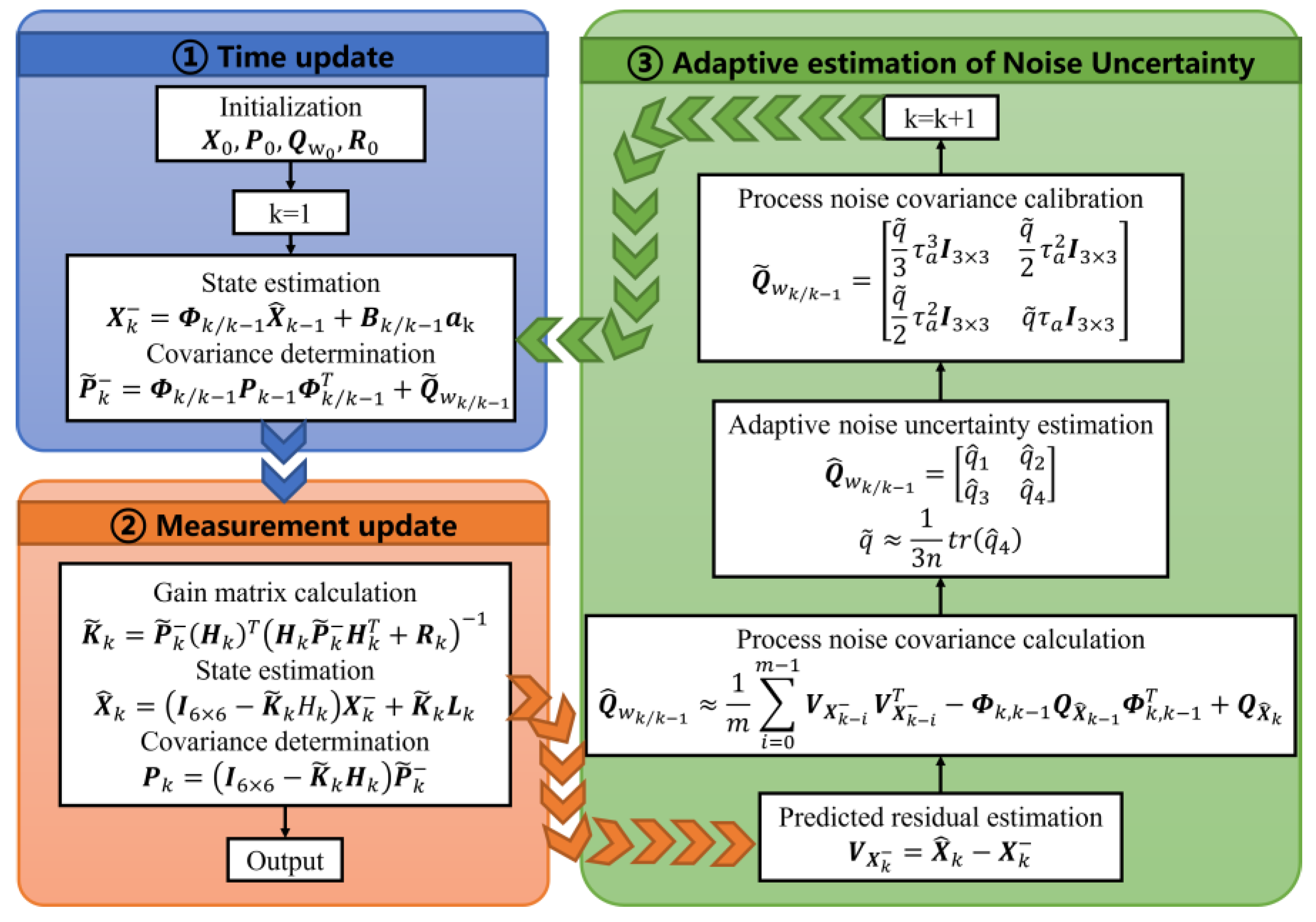
2.2. A Sage–Husa Kalman Filter Method with Adaptive Estimation of Strong Motion Acceleration Noise Uncertainty

Considering that there are significantly different errors introduced by the above-mentioned tilt, rotation, hysteresis, and non-linear instrument response at different stations or at different times at the same station, it is inappropriate to employ a fixed noise uncertainty for strong motion accelerations. To address this issue, a Sage–Husa Kalman filter method with adaptive estimation of strong motion acceleration noise uncertainty is proposed. In the proposed method, the noise uncertainty is adaptively estimated based on the Sage–Husa sliding-window estimation principle, at the same time the effect of baseline shift is accommodated through adaptive variance inflation.

Adaptive estimation of noise uncertainty allows the filter to dynamically adjust to changes in measurement conditions, making it suitable for applications where traditional fixed noise uncertainty assumptions may be inadequate. Consideration of baseline shift allows for a more accurate representation of the system’s process noise, and thereby enhances the filter performance.

The predicted residual of the state vector after the measurement update reads as follows:

$${\mathit{V}}_{{\mathit{X}}_k^{-}}={\widehat{\mathit{X}}}_k-{\mathit{X}}_k^{-}$$

(8)

Utilizing the law of variance–covariance propagation, the covariance matrix of the predicted residual can be expressed as follows:

$${\mathit{Q}}_{{\mathit{V}}_{{\mathit{X}}_k^{-}}}=Cov\left({\widehat{\mathit{X}}}_k-{\mathit{X}}_k^{-}\right)=Cov\left({\widehat{\mathit{X}}}_k\right)+Cov\left({\mathit{X}}_k^{-}\right)-2Cov\left({{\widehat{\mathit{X}}}_k,\mathit{X}}_k^{-}\right)$$

(9)

where $Cov\left(\cdot \right)$ represents the covariance operator. The covariance matrixes of ${\widehat{\mathit{X}}}_k$ and ${\mathit{X}}_k^{-}$, and their cross-term can be calculated as follows:

$$\left\{\begin{array}{c}Cov\left({\widehat{\mathit{X}}}_k\right)={\mathit{P}}_k\\ Cov\left({\mathit{X}}_k^{-}\right)={\mathit{P}}_k^{-}\\ Cov\left({{\widehat{\mathit{X}}}_k,\mathit{X}}_k^{-}\right)={\mathit{P}}_k^{-}-{\mathit{K}}_k{\mathit{H}}_k{\mathit{P}}_k^{-}\end{array}\right.$$

(10)

Combining Equation (9) with Equation (10), the covariance of the prediction residual can be reformulated as follows:

$${\mathit{Q}}_{{\mathit{V}}_{{\mathit{X}}_k^{-}}}={\mathit{P}}_k+{\mathit{P}}_k^{-}-2\left({\mathit{P}}_k^{-}-{\mathit{K}}_k{\mathit{H}}_k{\mathit{P}}_k^{-}\right)={\mathit{P}}_k^{-}-{\mathit{P}}_k$$

(11)

With ${\mathit{P}}_k={\mathit{Q}}_{{\widehat{\mathit{X}}}_k}$ defined, and substituting Equation (4) into Equation (11), the covariance of the prediction residual is calculated as follows:

$${\mathit{Q}}_{{\mathit{V}}_{{\mathit{X}}_k^{-}}}={\mathit{Q}}_{{\mathit{w}}_{k/k-1}}+{\mathit{\Phi }}_{k,k-1}{\mathit{Q}}_{{\widehat{\mathit{X}}}_{k-1}}{\mathit{\Phi }}_{k,k-1}^T-{\mathit{Q}}_{{\widehat{\mathit{X}}}_k}$$

(12)

Given the expectation $E\left({\mathit{V}}_{{\mathit{X}}_k^{-}}\right)=0$, the covariance matrix of ${\mathit{V}}_{{\mathit{X}}_k^{-}}$ can be approximately calculated by using historical predicted residuals in the sliding-window [51]:

$${\widehat{\mathit{Q}}}_{{\mathit{V}}_{{\mathit{X}}_k^{-}}}\approx \frac{1}{m}\sum _{i=0}^{m-1}{\mathit{V}}_{{\mathit{X}}_{k-i}^{-}}{\mathit{V}}_{{\mathit{X}}_{k-i}^{-}}^T$$

(13)

where $m$ stands for the number of acceleration records in the sliding-window.

When the system model maintains stability and consistency within the sliding window, the historical predicted residuals encapsulated by this window should accurately mirror the process noise level of the current state. Consequently, by integrating Equation (13) into Equation (12), the covariance matrix of process noise can also be approximately calculated as follows:

$${\widehat{\mathit{Q}}}_{{\mathit{w}}_{k/k-1}}\approx \frac{1}{m}\sum _{i=0}^{m-1}{\mathit{V}}_{{\mathit{X}}_{k-i}^{-}}{\mathit{V}}_{{\mathit{X}}_{k-i}^{-}}^T-{\mathit{\Phi }}_{k,k-1}{\mathit{Q}}_{{\widehat{\mathit{X}}}_{k-1}}{\mathit{\Phi }}_{k,k-1}^T+{\mathit{Q}}_{{\widehat{\mathit{X}}}_k}$$

(14)

Such an estimation encompasses both acceleration measurement noise and the impact of strong motion acceleration baseline shift. Historical predicted residuals in the recent period of time provide a more accurate reference for the noise level of strong motion acceleration. The ${\widehat{\mathit{Q}}}_{{\mathit{w}}_{k/k-1}}$ is introduced to encapsulate characteristics of the acceleration noise uncertainty, and can be represented as a block matrix:

$${\widehat{\mathit{Q}}}_{{\mathit{w}}_{k/k-1}}=\left[\begin{array}{cc}{\widehat{\mathit{q}}}_1& {\widehat{\mathit{q}}}_2\\ {\widehat{\mathit{q}}}_3& {\widehat{\mathit{q}}}_4\end{array}\right]$$

(15)

where ${\widehat{\mathit{q}}}_i\left(i=1,2,3,4\right)$ are 3 by 3 matrices. The trace of ${\widehat{\mathit{q}}}_4$ is represented by $tr\left({\widehat{\mathit{q}}}_4\right)$, which is a measure scale of the overall noise uncertainty of strong motion accelerations between two adjacent GNSS observation epochs.

Assuming that there are $n$ acceleration records between two adjacent GNSS observation epochs and the effect of a baseline shift for each acceleration record between two adjacent high-rate GNSS observation epochs is approximately uniform, the noise uncertainty of strong motion acceleration can be approximated as follows:

$$\tilde{q}\approx \frac{1}{3n}tr\left({\widehat{\mathit{q}}}_4\right)$$

(16)

The covariance matrix of the process noise for the next epoch is calculated by using adaptive estimation of noise uncertainty $\tilde{q}$, and it can be rewritten as follows:

$${\tilde{\mathit{Q}}}_{{\mathit{w}}_{k/k-1}}=\left[\begin{array}{cc}\frac{\tilde{q}}{3}{\tau }_a^3{\mathit{I}}_{3\times 3}& \frac{\tilde{q}}{2}{\tau }_a^2{\mathit{I}}_{3\times 3}\\ \frac{\tilde{q}}{2}{\tau }_a^2{\mathit{I}}_{3\times 3}& \tilde{q}{\tau }_a{\mathit{I}}_{3\times 3}\end{array}\right]$$

(17)

By applying the adaptive estimation ${\tilde{\mathit{Q}}}_{{\mathit{w}}_{k/k-1}}$ into Equations (4) and (5), the updated gain matrix is rewritten as follows:

$${\tilde{\mathit{K}}}_k={\tilde{\mathit{P}}}_k^{-}{\mathit{H}}_k^T{\left({\mathit{H}}_k{\tilde{\mathit{P}}}_k^{-}{\mathit{H}}_k^T+{\mathit{R}}_k\right)}^{-1}$$

(18)

where ${\tilde{\mathit{P}}}_k^{-}$ is the covariance matrix of predicted state vector based on the adaptive estimation of process noise. This can be expressed as the following equation:

$${\tilde{\mathit{P}}}_k^{-}={\mathit{\Phi }}_{k/k-1}{\mathit{P}}_{k-1}{\mathit{\Phi }}_{k/k-1}^T+{\tilde{\mathit{Q}}}_{{\mathit{w}}_{k/k-1}}$$

(19)

Combining the updated gain matrix ${\tilde{\mathit{K}}}_k$ with Equation (6), the state vector and its covariance matrix based on the adaptive estimation of strong motion acceleration noise uncertainty can be estimated by the following equations:

$${\widehat{\mathit{X}}}_k=\left({\mathit{I}}_{6\times 6}-{\tilde{\mathit{K}}}_k{\mathit{H}}_k\right){\mathit{X}}_k^{-}+{\tilde{\mathit{K}}}_k{\mathit{L}}_k$$

(20)

$${\mathit{P}}_k=\left({\mathit{I}}_{6\times 6}-{\tilde{\mathit{K}}}_k{\mathit{H}}_k\right){\mathit{P}}_k^{-}$$

(21)

Figure 1 illustrates the process flowchart of the Sage–Husa Kalman filter method with adaptive estimation of strong motion acceleration noise level. The process unfolds in three steps:

Step 1.

Time Update

The time update provides a prediction for the current state and covariance estimation ahead of time. The state estimation is determined based on the system’s dynamic model. The dynamic model incorporates the control input’s strong motion acceleration. And the covariance matrix is updated to reflect the process noise associated with the acceleration noise level of the control input.

Step 2.

Measurement Update

The measurement update refines the state and covariance estimations with new GNSS displacements. The gain matrix is calculated first, and this calculation determines the influences of new GNSS displacements on the state of estimation. Then the state estimation is updated by incorporating the GNSS displacements and the gain matrix. The covariance matrix is also updated to reflect the noise level of the GNSS displacement.

Step 3.

Adaptive Estimation of Noise Uncertainty

A sliding-window estimation is employed to compute the noise uncertainty of the strong motion acceleration. Concurrently, the effect of the baseline shift is accommodated through adaptive variance inflation. With the adaptive estimation of acceleration noise uncertainty in place, the covariance of process noise is then calibrated.

After each time update, measurement update, and adaptive estimation of the process noise level cycle, the process is repeated with the updated state estimation and covariance serving as the basis for the next time update step.

3. Experiments, Results and Discussion

3.1. Data Processing Strategy

To evaluate the performance of the proposed Sage–Husa Kalman filter method with adaptive estimation of strong motion acceleration noise uncertainty, two experiments including a shake table simulation experiment and an application to Mw 7.8 and Mw 7.6 earthquake doublet were carried out. The data processing strategy of strong motion acceleration and GNSS displacement before integration are outlined in

Table 1. Data processing strategies for GNSS displacement and strong motion acceleration before integration.

Items	Processing Information
Strong motion acceleration	De-mean the first 5 s from acceleration records
Covariance matrix of process noise	Determined by pre-event acceleration noises
GNSS displacement	Retrieved from TPP method
Covariance matrix of displacement noise	Determined by pre-event displacement noises

.

During the time update step, the acceleration recorded by a strong motion seismometer before an earthquake is not always zero. Such a phenomenon can be due to factors like initial adjustment errors or changes in environmental temperature. This non-zero acceleration value before the earthquake serves as the baseline initial value. If not corrected, it can lead to significant drifts in displacement waveforms after integration. Therefore, before integrating the GNSS displacement with the strong motion acceleration, the average acceleration value of 5 s before the earthquake was calculated as the initial baseline shift value. This value was deducted from the entire acceleration records to remove the initial baseline shift. These corrected accelerations served as the control input vectors. At the same time, the standard deviation of the pre-event acceleration records was calculated as the measuring noise uncertainty of the strong motion acceleration. The covariance matrix of the initial process noise was then determined by this measuring noise uncertainty. Concurrently, the coseismic displacements were recovered by double-integration of these corrected accelerations.

During the measurement update step, the GNSS-derived displacements were acquired using the TPP method. The underlying models, conventions, and strategies for the TPP approach have been detailed in our previous study [29]. The initial covariance matrix of GNSS displacement is also determined by pre-event noises. To highlight the benefits of integrating strong motion acceleration with GNSS displacement, the displacement derived from the GNSS TPP method and strong motion acceleration double-integration method are labeled as GNSS and Acc in the subsequent analysis.

For comparative purposes, the traditional Kalman filter method with empirically fixed noise was employed to validate the performance of the proposed method. The noise uncertainty of the traditional Kalman filter method was defined by referring to the multiplier selection strategy of Bock et al. [39]. The two processing schemes are presented in

Table 2. Two processing schemes.

Scheme	Method	Acceleration Noise Uncertainty
KF	Traditional Kalman filter method	Determined based on the pre-event noise with a multiplier
KF + ANUE	The proposed method	Adaptively estimated based on the Sage–Husa sliding-window estimation

. For the sake of convenience, these two processing schemes are sequentially denoted as KF and KF + ANUE in the following. The software for the integration of high-rate GNSS and strong motion records was programmed using the C language, following the methods of KF and KF + ANUE.

3.2. Result and Discussion

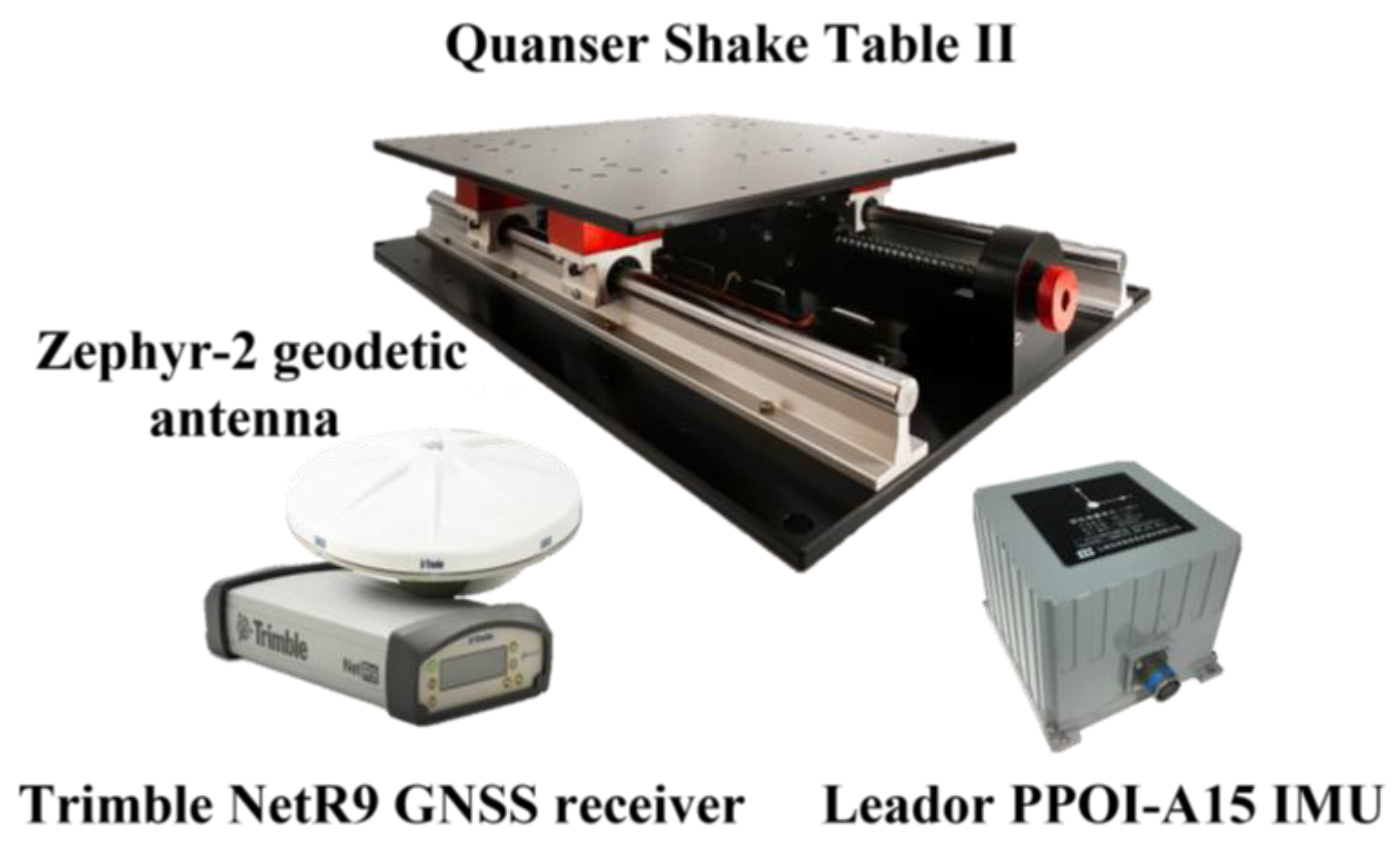
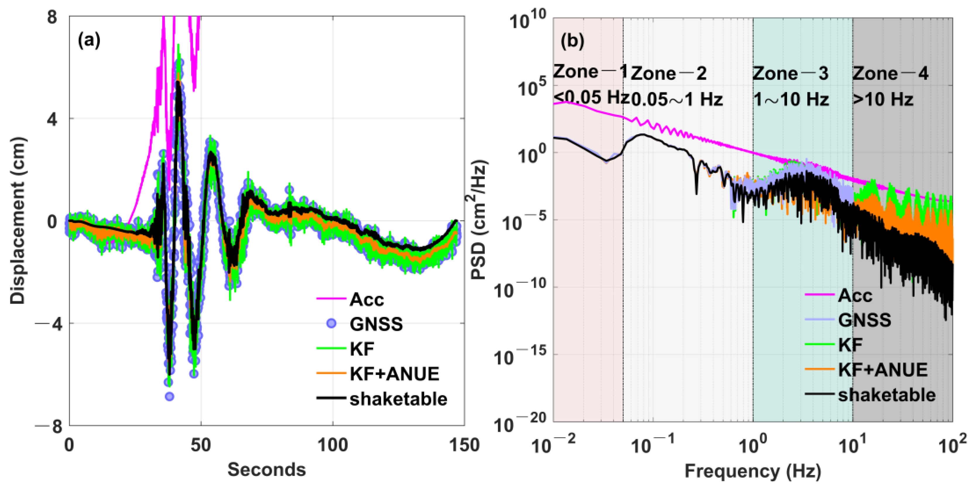
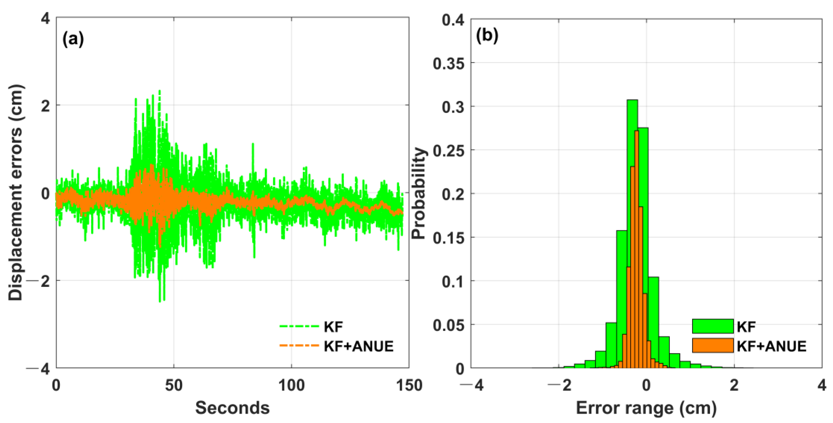
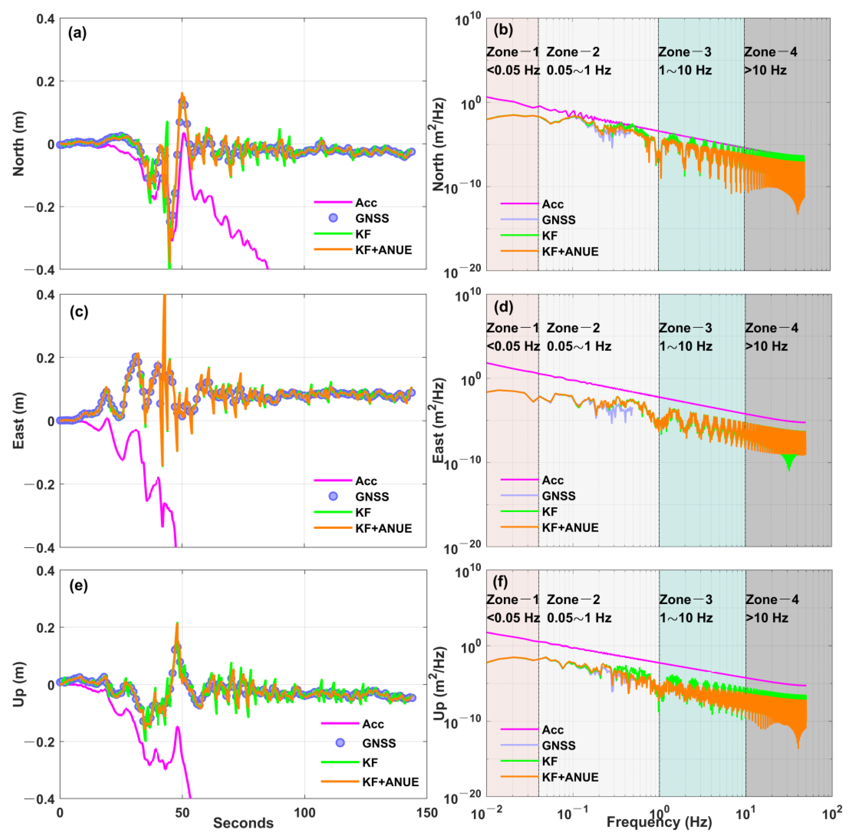
3.2.1. Shake Table Simulation Experiment

To validate the performance of the proposed integration method, we utilized a shake table dataset open accessed by Wuhan University [52]. In this dataset, a Quanser Shake Table II was applied to simulate the seismic waveforms of a real earthquake. The shake table is a middle-size, single-axis earthquake simulator that can generate pre-loaded acceleration profiles of real earthquakes for seismogeodesy research. Equipped with a high-resolution encoder, the shake table can measure stage position at a sampling rate of up to 2000 Hz with a resolution of 3.10 μm. This simulation experiment provided a controlled environment for testing the proposed method.

During the shake table simulation experiment, the north–south accelerometer recordings from the Mianzhu-Qingping station were utilized. This station is located 1 km away from the epicenter of the 2008 May 12 Mw 7.9 Wenchuan earthquake. The data duration was about 150 s, with a recorded peak acceleration of about 2 g and a peak-to-peak displacement of about 12 cm. The records of simulated seismic displacement waveform (abbreviated as shake table) can be measured by the embedded encoder, serving as the truth benchmarks of ground movement. GNSS observations were collected at a sampling rate of 20 Hz using a Trimble NetR9 GNSS receiver with a Zephyr-2 geodetic antenna installed on the platform. A Leador PPOI-A15 navigation-grade triaxial inertial measurement unit (IMU) firmly anchored at the platform were used to gather acceleration records at 200 Hz. Initially, the IMU was aligned to the east, north, and up directions and was utilized as a strong motion accelerometer. Figure 2 illustrates the equipment setup for the shake table experiment.

According to the aforementioned processing strategy, the 20 Hz GNSS observations and 200 Hz acceleration records were used to carry out displacement retrieval. Only the displacement in the north–south direction was involved in this assessment, in order to resemble the scene of a real earthquake occurrence more closely. Figure 3a presents the north–south oriented displacement waveforms after processing, which include Acc-derived, GNSS-derived, two integration solutions and shake table reference. The low-frequency noises are amplified in the Acc-derived displacement, and this leads to non-physical baseline drifts. This drift becomes larger and larger with the increase of integration time. Due to the mismatch of system model process noise, the filtered signal derived from the KF method exhibits unsmooth high-frequency oscillations resembling a sawtooth pattern. Compared to the traditional KF method, the KF + ANUE method exhibits better consistency with the shake table digital signal references. The effect of high-frequency sawtooth and baseline drifts is also suppressed.

To verify the characteristics of the proposed method in the frequency domain, the displacement power spectrum density (PSD) of the KF and KF + ANUE methods were calculated using the Welch algorithm [53], as shown in Figure 3b. In the low-frequency region below 1 Hz (Zone-1 and Zone-2), the PSD of KF and KF + ANUE is relatively consistent with the PSD of GNSS and shake table reference, indicating fewer errors in these frequency bands. In the frequency region above 1 Hz (Zone-3 and Zone-4), the displacement PSD of KF + ANUE is smaller than that obtained by the KF method, proving that the proposed method has a suppressive effect on high-frequency noise in coseismic displacement signals. The PSDs of the Acc displacement waveforms are larger than those of the GNSS, the KF + ANUE, and the shake table waveforms at the whole frequency domain, due to the effect of baseline shift.

The time series and histograms of the errors in computed displacement waveforms are further presented in Figure 4a,b, indicating the variability of their performance over the main shake period. The displacement retrieved from the KF + ANUE method exhibits a more stable and lower error range throughout the main shake period, which is indicative of its superior performance relative to the KF method. The error range for the KF method starts at approximately 0.01 cm and increases to around 2.48 cm over the course of 150 s. The KF + ANUE method maintains a lower error range, with values consistently below 1.23 cm, showcasing enhanced accuracy and stability. There is a visible trend in the KF method’s error, which suggests a potential systematic increase in error over time, whereas the KF + ANUE method’s error remains relatively flat, suggesting a robustness against time-varying effects of the baseline shift implicated in strong motion acceleration.

The root mean square error (RMSE) of the differences between the integrated displacement and the reference was calculated to verify the accuracy of the proposed method in this study. For a more rigorous analysis, we also computed the cross-correlation coefficient (CC) of each result related to the reference, as shown in

Table 3. The CC and RMSE for the integrated coseismic displacement.

Scheme	CC	RMSE (cm)
KF	0.95	0.45
KF + ANUE	0.99	0.32

. When the KF method is employed, the accuracy of the derived displacement is determined to be 0.45 cm, with the CC values reaching a level of 0.95. In contrast to the KF method, the displacement derived from the KF + ANUE method demonstrated superior alignment with the digital signal references obtained from the shake table. This enhanced consistency is evidenced by its exceptional CC of 0.99 and an RMSE of 0.32 cm for the displacement derived from the KF + ANUE method. The KF + ANUE method signifies a substantial improvement of up to 28% over the KF method in terms of displacement accuracy.

These preliminary validations indicate that the proposed method can provide broadband and more accurate displacement waveforms compared with the KF method. The historical predicted residuals in the recent period of time can be applied to provide a more accurate reference for the noise level of strong motion acceleration. This advancement is particularly significant in the context of seismic event analysis, where the fidelity of displacement retrieval is paramount for precise seismic waveform capture and seismic rupture propagation.

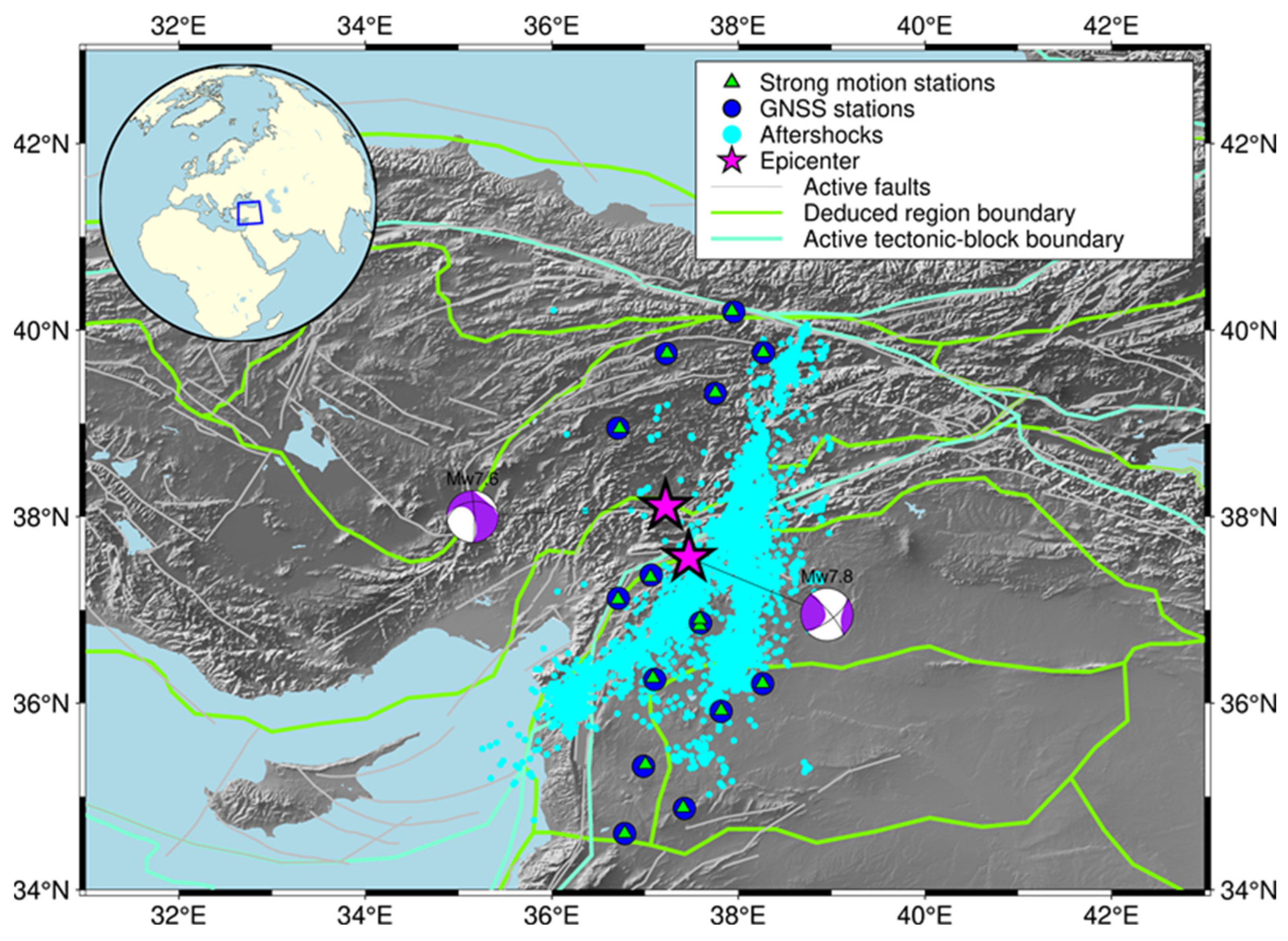
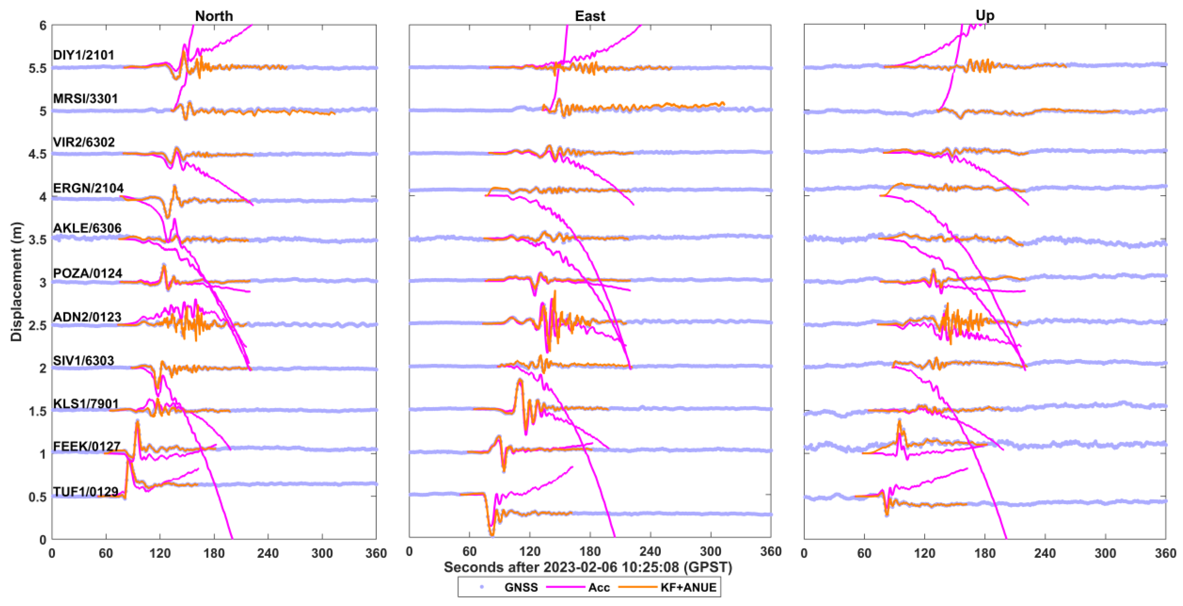
3.2.2. Application to Mw 7.8 and Mw 7.6 Earthquake Doublet

To further validate the performance of the proposed KF + ANUE method for the application of real earthquake events, a representative example of a real historical earthquake is indispensable. On 6 February 2023, an earthquake doublet with magnitudes of Mw 7.8 and Mw 7.6 struck the East Anatolian Fault Zone, causing significant damage to civil and infrastructure throughout southeast Turkey and northwest Syria [54]. The entire main shaking process was successfully recorded by a dense network of high-rate GNSS with a sample rate of 1 Hz and strong motion stations operating at a sampling rate of 100 Hz. These data can be obtained from https://www.tusaga-aktif.gov.tr/, accessed on 25 March 2024.

We defined a collection of seismometers positioned within 5 km of each other as a pair. It is generally observed that seismic waveforms derived from GNSS and strong motion accelerometers remain consistent with each other for seismometer separations of less than 15 km [2]. Following this guideline, we identified 15 suitable co-locations in this contribution, with a separation distance ranging from 0.02 km to 3.37 km. The basic information about those co-located station pairs is provided in

Table 4. Information on collected high-rate GNSS stations and strong motion seismometer stations.

Station	Latitude (°N)	Longitude (°E)	Dist to Epic 1 (km)	Separation Distance (km)
ANTE/2703	37.06	37.37	38.74	2.23
MAR1/4617	37.59	36.86	49.92	2.89
MAR1/4620	37.59	36.86	49.92	3.37
ONIY/8003	37.10	36.25	61.95	2.43
TUF1/0129	38.26	36.21	87.30	0.26
FEEK/0127	37.81	35.91	110.51	0.72
KLS1/7901	36.71	37.12	143.17	1.10
SIV1/6303	37.75	39.32	192.57	0.66
ADN2/0123	36.98	35.32	196.85	2.87
POZA/0124	37.40	34.87	210.46	1.63
AKLE/6306	36.71	38.95	214.09	1.97
ERGN/2104	38.27	39.76	230.07	0.58
VIR2/6302	37.22	39.75	244.56	0.98
MRSI/3301	36.78	34.60	262.70	0.02
DIY1/2101	37.95	40.19	266.92	2.32

¹ Dist to epic stands for distance from station location to epicenter location.

, and the distribution of co-located station pairs is shown in Figure 5. Following the processing strategy described in Section 3.1, the 1 Hz GNSS observations and 100 Hz acceleration records were processed to retrieve three-direction displacements for the Mw 7.8 and Mw 7.6 earthquake doublet in southeast Turkey and northwest Syria. The calculation period is set to more than 2 min, covering the main shake period. The accuracy of the displacements derived from the proposed method is assessed by taking the results obtained from PRIDE PPP-AR software ver. 3.0 developed by Wuhan University as references [55].

The left subgraphs in Figure 6 show the coseismic displacement of a typical station, SIV1/6303, in the east, north, and up directions during the first Mw 7.8 earthquake, respectively. This station is situated at a distance of 192.57 km from the epicenter of the same earthquake. The seismic signals recorded at this station are relatively complete. The “0” value on the horizontal axis signifies the moment the main shock occurred. Before the seismic waves arrive, the integrated displacements from the KF and KF + ANUE methods closely align with the GNSS-derived displacement. As the seismic waves propagate and the station experiences escalating shaking, the displacements derived from KF and KF + ANUE methods continue to track the general trend observed in the GNSS. In contrast, the displacements of Acc scheme exhibit non-physical drifts, which can be attributed to the impact of baseline shifts. The smoothness of the displacement waveforms across the KF and KF + ANUE methods is notably inconsistent. The high-frequency sawtooth evident in the displacement of KF and KF + VCE methods is less pronounced in the KF + ANUE scheme. Among these methods, KF + ANUE demonstrated the highest degree of congruence with the GNSS-derived displacement at equivalent time intervals, particularly as compared to the KF method. The baseline drift displayed in the Acc-derived displacement is also eliminated in the result of KF + ANUE.

To investigate the integration method in the frequency domain, the right subgraphs of Figure 6 show the PSDs of the GNSS-derived, Acc-derived, and integrated displacements of SIV1/6303 in the north, east, and up directions, respectively. The PSDs of the waveforms derived from the KF + ANUE demonstrate a greater alignment with those of the GNSS waveforms at low frequencies, below 1 Hz (Zone-1 and Zone-2), especially in the north and up directions. In the frequency band region above 1 Hz (Zone-3 and Zone-4), the displacement PSD of KF + ANUE is smaller than that obtained by the KF method. It means the high-frequency noises in coseismic displacement signals are effectively suppressed by the proposed method due to the adaptive variance inflation, which is similar to the results displayed in the shake table experiments.

Coseismic displacement waveforms of KF exhibit their disadvantages as in our previous analyses. The displacement waveforms derived from the KF + ANUE method can avoid the drawbacks and preserve the benefits of GNSS and strong motion records, providing broadband displacements with a high-precision level. To depict seismic rupture propagation, Figure 7 and Figure 8 present the displacement waveforms derived from the KF + ANUE method for 11 available station pairs during the Mw 7.8 and Mw 7.6 earthquake doublet, respectively. Displacements derived solely from GNSS and strong motion seismometers are also presented for comparison. It should be noticed that the coseismic displacements of each station are vertically shifted according to the epicentral distance. Displacement waveforms from GNSS and KF + ANUE remained generally consistent until data transmissions from the MAR1 and AKLE stations were disrupted. However, due to the absence of subsequent GNSS displacements, the effectiveness of integrated displacement throughout the earthquake remains undetermined. At station ONIY/8003, located 61.95 km from the hypocenter, the integrated displacement waveform exhibits two ambiguous phases of seismic energy release, attributable to permanent ground displacement. The remaining eight station pairs recorded coseismic displacement waveforms throughout the earthquake, with no significant systematic deviation observed between GNSS-derived displacements and those obtained via the KF + ANUE method.

Similar to the results of the first Mw 7.8 earthquake, Figure 8 displays the KF + ANUE integrated displacement sequences of 11 available station pairs in the second Mw 7.6 earthquake. Due to damage caused by the strong earthquake, four station pairs are different from those in the first earthquake case. Prior to the seismic wave’s arrival, the integrated displacement aligns closely with that recorded by strong motion seismometers. Following the wave’s arrival, the integrated displacement mirrors the result of GNSS, albeit with shake amplitudes less than those of identical station pairs in the first event, remaining under 40 cm. In general terms, GNSS displacements suffer from low sampling rates and high noise levels, failing to capture seismic wave signals in detail. Strong motion seismometers, despite their high sampling rates, exhibit significant drift post-integration. The proposed method has greater superiority over these two single observing techniques.

Table 5. The mean CC and RMSE (cm) for the retrieved coseismic displacements in the Mw 7.8 and Mw 7.6 earthquake doublet.

Scheme	The First Mw 7.8 Event						The Second Mw 7.6 Event
	CC			RMSE (cm)			CC			RMSE (cm)
	North	East	Up	North	East	Up	North	East	Up	North	East	Up
KF	0.85	0.87	0.86	2.24	1.92	2.11	0.93	0.90	0.93	1.44	1.72	1.47
KF + ANUE	0.95	0.98	0.91	1.31	1.02	1.64	0.95	0.93	0.94	1.33	1.43	1.35

provides a quantitative analysis of the KF + ANUE method’s performance in capturing seismic wave displacements. The mean CC and RMSE for co-located GNSS and strong motion station pairs during the Mw 7.8 and Mw 7.6 earthquake doublet are presented. Compared to the KF scheme, displacements derived from the KF + ANUE method demonstrated superior performance in terms of both accuracy and signal correlation for the Mw 7.8 and Mw 7.6 earthquake doublet. For the Mw 7.8 event, the KF method achieves accuracies of 2.24 cm, 1.92 cm, and 2.11 cm in their respective directions, with corresponding CC values of 0.85, 0.87, and 0.86. The CC values for the KF + ANUE method both exceeded 0.90 in all three directions. Conversely, the KF + ANUE method achieves displacement extraction accuracies of 1.31 cm, 1.02 cm, and 1.64 cm in the north, east, and up directions, respectively. This represents an improvement of up to 44% in the horizontal direction and 22% in the vertical direction over the KF method.

Mirroring its accuracy in the preceding event, the proposed method can retrieve displacement for the Mw 7.6 event with remarkable precision. It achieved accuracies of 1.33 cm, 1.43 cm, and 1.35 cm in the north, east, and up directions, respectively. The CC values for the KF + ANUE method average at 0.94 in the horizontal and vertical directions. In comparison, the KF method’s performance in these directions is marked by accuracies of 1.44 cm, 1.72 cm, and 1.47 cm, respectively. The average CC value for the three directions is 0.92. While there are only minor differences in the accuracies of displacements retrieved from the KF and KF + ANUE methods in the north and up directions, a significant improvement was observed in the displacements in the east direction during the second Mw 7.6 earthquake. Despite these nuances, the proposed method exhibits an overall improvement of up to 12% in the horizontal direction and 8% in the vertical direction as compared to the KF method.

By synthesizing the accuracy of two distinct events, the proposed method significantly enhances the capture of seismic waveforms, showing improvements of 46% in the horizontal direction and 23% in the vertical direction over the outcomes of the KF method. The above results show that the proposed method can provide much more precise coseismic displacement than the KF method. These integrated displacements of the collected GNSS and strong motion stations are consistent with the reference displacement values processed by PRIDE PPP-AR software.

In a word, the KF + ANUE method markedly outperforms the KF method by adaptively estimating the noise uncertainty of strong motion acceleration utilizing the Sage–Husa sliding-window estimation principle. In the pre-filtering and mid-filtering stages, the influences of baseline shift were accommodated through adaptive variance inflation, thereby eliminating the drift in seismic signals effectively. In the later filtering stages, GNSS-derived displacements significantly constrained the integration results, enabling accurate recording of seismic waves’ low-frequency information. Despite being approximately 200 km from the epicenter, stations like POZA/0124 and five others successfully detected seismic signals. The proposed method combines the strengths of both GNSS and strong motion seismometers, ensuring comprehensive seismic signal capture without divergence throughout the earthquake event.

4. Conclusions

In this paper, we present a Sage–Husa Kalman filter method, where the noise uncertainty of strong motion acceleration is adaptively estimated to integrate GNSS and strong motion for obtaining displacement series. The broadband displacement waveforms in a great earthquake can be achieved by using the proposed method. Compared with the traditional Kalman filter method, historical predicted residuals in the recent times are applied to provide a more accurate reference for the noise level of strong motion acceleration. The noise uncertainty of strong motion acceleration is adaptively determined utilizing the Sage–Husa sliding-window estimation principle, at the same time the effect of the baseline shift is accommodated through adaptive variance inflation. This method significantly improved the accuracy of the system’s process noise representation, and thereby improved filter performance. The performance of the proposed method was assessed through a shake table simulation experiment and by analyzing data from GNSS/strong motion co-located stations during the 2023 Mw 7.8 and Mw 7.6 earthquake doublet in Southeast Turkey. The results indicate that the method significantly improves adaptability to variations in strong motion accelerometer noises and enhances accuracy of the integrated displacement series. Specifically, in the shake table test, the proposed method retrieved the displacements with an accuracy of 0.32 cm. This represents an improvement of up to 28% over the traditional Kalman filter method. The displacement waveforms derived from the proposed method achieved a correlation coefficient of 0.99 with respect to reference values, outperforming the traditional Kalman filter method by a margin of 0.04. These increases in the retrieval accuracy and correlation coefficient signify a notably more accurate alignment with the benchmark signal. When applied to the earthquake event, the proposed method demonstrated an ability to capture seismic waveforms with an improvement of 46% and 23% in the horizontal and vertical directions, respectively, as compared with the traditional Kalman filter-based results. This contribution shows that the proposed method can provide a more accurate estimation of broadband displacement waveforms to support earthquake early warning and rapid response in a great earthquake.

References

1. Saunders, J.K.; Goldberg, D.E.; Haase, J.S.; Bock, Y.; Offield, D.G.; Melgar, D.; Restrepo, J.; Fleischman, R.B.; Nema, A.; Geng, J.; et al. Seismogeodesy Using GPS and Low-Cost MEMS Accelerometers: Perspectives for Earthquake Early Warning and Rapid Response. Bull. Seismol. Soc. Am. 2016, 106, 2469–2489. [Google Scholar] [CrossRef]
2. Emore, G.L.; Haase, J.S.; Choi, K.; Larson, K.M.; Yamagiwa, A. Recovering Seismic Displacements through Combined Use of 1-Hz GPS and Strong-Motion Accelerometers. Bull. Seismol. Soc. Am. 2007, 97, 357–378. [Google Scholar] [CrossRef]
3. Dahmen, N.; Hohensinn, R.; Clinton, J. Comparison and Combination of GNSS and Strong-Motion Observations: A Case Study of the 2016 Mw 7.0 Kumamoto Earthquake. Bull. Seismol. Soc. Am. 2020, 110, 2647–2660. [Google Scholar] [CrossRef]
4. Iwan, W.D.; Moser, M.A.; Peng, C.Y. Some Observations on Strong-Motion Earthquake Measurement Using a Digital Accelerograph. Bull. Seismol. Soc. Am. 1985, 75, 1225–1246. [Google Scholar] [CrossRef]
5. Boore, D.M. Comments on Baseline Correction of Digital Strong-Motion Data: Examples from the 1999 Hector Mine, California, Earthquake. Bull. Seismol. Soc. Am. 2002, 92, 1543–1560. [Google Scholar] [CrossRef]
6. Boore, D.M.; Bommer, J.J. Processing of strong-motion accelerograms: Needs, options and consequences. Soil Dyn. Earthq. Eng. 2005, 25, 93–115. [Google Scholar] [CrossRef]
7. Wu, Y.M.; Wu, C.F. Approximate Recovery of Coseismic Deformation from Taiwan Strong-Motion Records. J. Seismol. 2007, 11, 159–170. [Google Scholar] [CrossRef]
8. Chao, W.A.; Wu, Y.M.; Zhao, L. An Automatic Scheme for Baseline Correction of Strong-Motion Records in Coseismic Deformation Determination. J. Seismol. 2010, 14, 495–504. [Google Scholar] [CrossRef]
9. Wang, R.; Schurr, B.; Milkereit, C.; Shao, Z.; Jin, M.P. An Improved Automatic Scheme for Empirical Baseline Correction of Digital Strong-Motion Records. Bull. Seismol. Soc. Am. 2011, 101, 2029–2044. [Google Scholar] [CrossRef]
10. Larson, K.M.; Bodin, P.; Gomberg, J. Using 1-Hz GPS Data to Measure Deformations Caused by the Denali Fault Earthquake. Science 2003, 300, 1421–1424. [Google Scholar] [CrossRef]
11. Li, X.; Ge, M.; Zhang, X.; Zhang, Y.; Guo, B.; Wang, R.; Klotz, J.; Wickert, J. Real-time high-rate co-seismic displacement from ambiguity-fixed precise point positioning: Application to earthquake early warning. Geophys. Res. Lett. 2013, 40, 295–300. [Google Scholar] [CrossRef]
12. Fang, R.; Shi, C.; Song, W.; Wang, G.; Liu, J. Determination of earthquake magnitude using GPS displacement waveforms from real-time precise point positioning. Geophys. J. Int. 2014, 196, 461–472. [Google Scholar] [CrossRef]
13. Bock, Y.; Nikolaidis, R.M.; de Jonge, P.J.; Bevis, M. Instantaneous geodetic positioning at medium distances with the Global Positioning System. J. Geophys. Res. 2000, 105, 28223–28253. [Google Scholar] [CrossRef]
14. Bock, Y.; Prawirodirdjo, L.; Melbourne, T.I. Detection of arbitrarily large dynamic ground motions with a dense high-rate GPS network. Geophys. Res. Lett. 2004, 31, L06604. [Google Scholar] [CrossRef]
15. Ohta, Y.; Kobayashi, T.; Tsushima, H.; Miura, S.; Hino, R.; Takasu, T.; Fujimoto, H.; Iinuma, T.; Tachibana, K.; Demachi, T.; et al. Quasi real-time fault model estimation for near-field tsunami forecasting based on RTK-GPS analysis: Application to the 2011 Tohoku-Oki earthquake (Mw 9.0). J. Geophys. Res. Solid Earth 2012, 117, B02311. [Google Scholar] [CrossRef]
16. Kouba, J. Measuring Seismic Waves Induced by Large Earthquakes with GPS. Stud. Geophys. Geod. 2003, 47, 741–755. [Google Scholar] [CrossRef]
17. Shi, C.; Lou, Y.; Zhang, H.; Zhao, Q.; Geng, J.; Wang, R.; Fang, R.; Liu, J. Seismic deformation of the Mw 8.0 Wenchuan earthquake from high-rate GPS observations. Adv. Space Res. 2010, 46, 228–235. [Google Scholar] [CrossRef]
18. Li, X.; Ge, M.; Lu, C.; Zhang, Y.; Wang, R.; Wickert, J.; Schuh, H. High-Rate GPS Seismology Using Real-Time Precise Point Positioning with Ambiguity Resolution. IEEE Trans. Geosci. Remote Sens. 2014, 52, 6165–6180. [Google Scholar] [CrossRef]
19. Chen, G.; Zhao, Q. Near-field surface displacement and permanent deformation induced by the Alaska Mw 7.5 earthquake determined by high-rate real-time ambiguity-fixed PPP solutions. Chin. Sci. Bull. 2014, 59, 4781–4789. [Google Scholar] [CrossRef]
20. Li, X.; Li, X.; Yuan, Y.; Zhang, K.; Zhang, X.; Wickert, J. Multi-GNSS phase delay estimation and PPP ambiguity resolution: GPS, BDS, GLONASS, Galileo. J. Geod. 2018, 92, 579–608. [Google Scholar] [CrossRef]
21. Collins, P.; Henton, J.; Mireault, Y.; Heroux, P.; Schmidt, M.; Dragert, H.; Bisnath, S. Precise point positioning for real-time determination of co-seismic crustal motion. In Proceedings of the ION GNSS 2009, Savannah, GA, USA, 22–25 September 2009; pp. 2479–2488. [Google Scholar]
22. Colosimo, G.; Crespi, M.; Mazzoni, A. Real-time GPS seismology with a stand-alone receiver: A preliminary feasibility demonstration. J. Geophys. Res. Solid Earth 2011, 116, B11302. [Google Scholar] [CrossRef]
23. Geng, T.; Xie, X.; Fang, R.; Su, X.; Zhao, Q.; Liu, G.; Li, H.; Shi, C.; Liu, J. Real-time capture of seismic waves using high-rate multi-GNSS observations: Application to the 2015 Mw 7.8 Nepal earthquake. Geophys. Res. Lett. 2016, 43, 161–167. [Google Scholar] [CrossRef]
24. Shu, Y.; Fang, R.; Li, M.; Shi, C.; Li, M.; Liu, J. Very high-rate GPS for measuring dynamic seismic displacements without aliasing: Performance evaluation of the variometric approach. GPS Solut. 2018, 22, 121. [Google Scholar] [CrossRef]
25. Li, X.; Ge, M.; Guo, B.; Wickert, J.; Schuh, H. Temporal point positioning approach for real-time GNSS seismology using a single receiver. Geophys. Res. Lett. 2013, 40, 5677–5682. [Google Scholar] [CrossRef]
26. Li, X.; Guo, B.; Lu, C.; Ge, M.; Wickert, J.; Schuh, H. Real-time GNSS seismology using a single receiver. Geophys. J. Int. 2014, 198, 72–89. [Google Scholar] [CrossRef]
27. Guo, B.; Zhang, X.; Ren, X.; Li, X. High-precision coseismic displacement estimation with a single-frequency GPS receiver. Geophys. J. Int. 2015, 202, 612–623. [Google Scholar] [CrossRef]
28. Chen, K.; Ge, M.; Babeyko, A.; Li, X.; Diao, F.; Tu, R. Retrieving real-time co-seismic displacements using GPS/GLONASS: A preliminary report from the September 2015 Mw 8.3 Illapel earthquake in Chile. Geophys. J. Int. 2016, 206, 941–953. [Google Scholar] [CrossRef]
29. Zhang, Y.; Nie, Z.; Wang, Z.; Wu, H.; Xu, X. Real-Time Coseismic Displacement Retrieval Based on Temporal Point Positioning with IGS RTS Correction Products. Sensors 2021, 21, 334. [Google Scholar] [CrossRef] [PubMed]
30. Genrich, J.F.; Bock, Y. Instantaneous geodetic positioning with 10–50 Hz GPS measurements: Noise characteristics and implications for monitoring networks. J. Geophys. Res. Solid Earth 2006, 1111, B03403. [Google Scholar] [CrossRef]
31. Larson, K.M.; Bilich, A.; Axelrad, P. Improving the precision of high-rate GPS. J. Geophys. Res. 2007, 112, B05422. [Google Scholar] [CrossRef]
32. Gao, Z.; Li, Y.; Shan, X.; Zhu, C. Earthquake Magnitude Estimation from High-Rate GNSS Data: A Case Study of the 2021 Mw 7.3 Maduo Earthquake. Remote Sens. 2021, 13, 4478. [Google Scholar] [CrossRef]
33. Li, Z.; Zang, J.; Fan, S.; Wen, Y.; Xu, C.; Yang, F.; Peng, X.; Zhao, L.; Zhou, X. Real-Time Source Modeling of the 2022 Mw 6.6 Menyuan, China Earthquake with High-Rate GNSS Observations. Remote Sens. 2022, 14, 5378. [Google Scholar] [CrossRef]
34. Boore, D.M. Effect of Baseline Corrections on Displacements and Response Spectra for Several Recording of the 1999 Chi-Chi, Taiwan, Earthquake. Bull. Seismol. Soc. Am. 2001, 91, 1199–1211. [Google Scholar] [CrossRef]
35. Wang, R.; Parolai, S.; Ge, M.; Jin, M.P.; Walter, T.R.; Zschau, J. The 2011 Mw 9.0 Tohoku earthquake: Comparison of GPS and strong-motion data. Bull. Seismol. Soc. Am. 2013, 103, 1336–1347. [Google Scholar] [CrossRef]
36. Tu, R.; Wang, R.; Ge, M.; Walter, T.R.; Ramatschi, M.; Milkereit, C.; Bindi, D.; Dahm, T. Cost-effective monitoring of ground motion related to earthquakes, landslides, or volcanic activity by joint use of a single-frequency GPS and a MEMS accelerometer. Geophys. Res. Lett. 2013, 40, 3825–3829. [Google Scholar] [CrossRef]
37. Melgar, D.; Bock, Y.; Sanchez, D.; Crowell, B.W. On robust and reliable automated baseline corrections for strong motion seismology. J. Geophys. Res. Solid Earth 2013, 118, 1177–1187. [Google Scholar] [CrossRef]
38. Smyth, A.; Wu, M. Multi-rate Kalman filtering for the data fusion of displacement and acceleration response measurements in dynamic system monitoring. Mech. Syst. Signal Process. 2007, 21, 706–723. [Google Scholar] [CrossRef]
39. Bock, Y.; Melgar, D.; Crowell, B.W. Real-Time Strong-Motion Broadband Displacements from Collocated GPS and Accelerometers. Bull. Seismol. Soc. Am. 2011, 101, 2904–2925. [Google Scholar] [CrossRef]
40. Song, C.; Xu, C. Loose integration of high-rate GPS and strong motion data considering coloured noise. Geophys. J. Int. 2018, 215, 1530–1539. [Google Scholar] [CrossRef]
41. Shu, Y.; Fang, R.; Geng, J.; Zhao, Q.; Liu, J. Broadband Velocities and Displacements From Integrated GPS and Accelerometer Data for High-Rate Seismogeodesy. Geophys. Res. Lett. 2018, 45, 8939–8948. [Google Scholar] [CrossRef]
42. Geng, J.; Bock, Y.; Melgar, D.; Crowell, B.W.; Haase, J.S. A new seismogeodetic approach applied to GPS and accelerometer observations of the 2012 Brawley seismic swarm: Implications for earthquake early warning. Geochem. Geophys. Geosyst. 2013, 14, 2124–2142. [Google Scholar] [CrossRef]
43. Li, X.; Ge, M.; Zhang, Y.; Wang, R.; Klotz, J.; Wicket, J. High-rate coseismic displacements from tightly-integrated processing of raw GPS and accelerometer data. Geophys. J. Int. 2013, 195, 612–624. [Google Scholar] [CrossRef]
44. Tu, R.; Ge, M.; Wang, R.; Walter, T.R. A new algorithm for tight integration of real-time GPS and strong-motion records, demonstrated on simulated, experimental, and real seismic data. J. Seismol. 2014, 18, 151–161. [Google Scholar] [CrossRef]
45. Guo, B.; Di, M.; Song, F.; Li, J.; Shi, S.; Limsupavanich, N. Integrated coseismic displacement derived from high-rate GPS and strong-motion seismograph: Application to the 2017 Ms 7.0 Jiuzhaigou Earthquake. Measurement 2021, 182, 109735. [Google Scholar] [CrossRef]
46. Fang, R.; Zheng, J.; Shu, Y.; Lv, H.; Shi, C.; Liu, J. A new tightly coupled method for high-rate seismogeodesy: A shake table experiment and application to the 2016 Mw 6.6 central Italy earthquake. Geophys. J. Int. 2021, 227, 1846–1856. [Google Scholar] [CrossRef]
47. Xin, S.; Geng, J.; Zeng, R.; Zhang, Q.; Ortega-Culaciati, F.; Wang, T. In-situ real-time seismogeodesy by integrating multi-GNSS and accelerometers. Measurement 2021, 179, 109453. [Google Scholar] [CrossRef]
48. Chen, C.; Lin, X.; Li, W.; Cheng, L.; Wang, H.; Zhang, Q.; Wang, Z. Adaptive coloured noise multirate Kalman filter and its application in coseismic deformations. Geophys. J. Int. 2023, 234, 1236–1253. [Google Scholar] [CrossRef]
49. Jing, C.; Huang, G.; Zhang, Q.; Li, X.; Bai, Z.; Du, Y. GNSS/Accelerometer Adaptive Coupled Landslide Deformation Monitoring Technology. Remote Sens. 2023, 14, 3537. [Google Scholar] [CrossRef]
50. Paziewski, J.; Stepniak, K.; Sieradzki, R.; Yigit, C.O. Dynamic displacement monitoring by integrating high-rate GNSS and accelerometer: On the possibility of downsampling GNSS data at reference stations. GPS Solut. 2023, 27, 157. [Google Scholar] [CrossRef]
51. Jing, C.; Huang, G.; Li, X.; Zhang, Q.; Yang, H.; Zhang, K.; Liu, G. GNSS/accelerometer integrated deformation monitoring algorithm based on sensors adaptive noise modeling. Measurement 2023, 179, 113179. [Google Scholar] [CrossRef]
52. Geng, J.; Wen, Q.; Zhang, T.; Li, C. Strong-motion seismogeodesy by deeply coupling GNSS receivers with inertial measurement units. Geophys. Res. Lett. 2020, 47, e2020GL087161. [Google Scholar] [CrossRef]
53. Qu, X.; Ding, X.; Xu, Y.; Yu, W. Real-time outlier detection in integrated GNSS and accelerometer structural health monitoring systems based on a robust multi-rate Kalman filter. J. Geod. 2023, 97, 38. [Google Scholar] [CrossRef]
54. Liu, C.; Lay, T.; Wang, R.; Taymaz, T.; Xie, Z.; Xiong, X.; Irmak, T.S.; Kahraman, M.; Erman, C. Complex multi-fault rupture and triggering during the 2023 earthquake doublet in southeastern Türkiye. Nat. Commun. 2023, 14, 5564. [Google Scholar] [CrossRef] [PubMed]
55. Geng, J.; Chen, X.; Pan, Y.; Mao, S.; Li, C.; Zhou, J.; Zhang, K. PRIDE PPP-AR: An open-source software for GPS PPP ambiguity resolution. GPS Solut. 2019, 23, 91. [Google Scholar] [CrossRef]
Figure 1. Flowchart of the Sage–Husa Kalman filter method with adaptive noise uncertainty estimation.
Remotesensing 16 02000 g001
Figure 2. The equipment setup for the shake table experiment.
Remotesensing 16 02000 g002
Figure 3. (a,b) Displacement time series and PSDs in the shake table experiment. (a) illustrates the time series of the integrated displacements. (b) showcases the PSDs of the integrated displacements.
Remotesensing 16 02000 g003
Figure 4. (a,b) Time series and histograms of the integrated displacement errors. (a) depicts the time series of the integrated displacement errors. (b) displays the distribution of the integrated displacement errors.
Remotesensing 16 02000 g004
Figure 5. Location of the co-located high-rate GNSS and strong motion seismometer stations collected during the Mw 7.8 and Mw 7.6 earthquake doublet.
Remotesensing 16 02000 g005
Figure 6. (af) Displacements and PSDs at the co-located station pair SIV1/6303 during the first Mw 7.8 earthquake. (a,c,e) illustrate the displacements of North, East and Up directions, respectively. (b,d,f) depict the displacement PSDs of North, East and Up directions, respectively.
Remotesensing 16 02000 g006
Figure 7. Coseismic displacements at 11 station pairs during the first Mw 7.8 earthquake.
Remotesensing 16 02000 g007
Figure 8. Coseismic displacements at 11 station pairs during the second Mw 7.6 earthquake.
Remotesensing 16 02000 g008