Abstract
The feedback of vegetation on cloud cover is an important link in the global water cycle. However, the relative importance of vegetation and related factors (surface properties, heat fluxes, and environmental conditions) on cloud cover in the context of greening remains unclear. Combining the Global Land Surface Satellite (GLASS) leaf area index (LAI) product and the fifth-generation reanalysis data of the European Centre for Medium-Range Weather Forecasts (ERA5), we quantified the relative contribution of vegetation and related factors to total cloud cover (TCC) in typical regions (Eastern European Plain, Western Siberian Plain, Mongolian Plateau, and Northeastern China Plain) of Eurasia over 21 years, and investigated how vegetation moderated the contribution of the other factors. Here, we show that the relative contribution of different factors to TCC was closely related to the climate and vegetation characteristics. In energy-limited (moisture-limited) areas, temperature (relative humidity) was more likely to be the factor that strongly contributed to TCC variation. Except for sparsely vegetated ecosystems, the relative contribution of LAI to TCC was stable within a range of 8–13%. The case study also shows that vegetation significantly modulated the contribution of other factors on TCC, but the degree of the regulation varied among different ecosystems. Our results highlight the important influence of vegetation on cloud cover during greening, especially the moderating role of vegetation on the contribution of other factors.
1. Introduction
Recent studies have revealed that vegetation has significant impacts on clouds [1,2,3]. It is well known that clouds are closely related to the hydrological cycle, surface radiation balance, and planetary albedo; thus, the importance of clouds in climate assessment is self-evident. In recent years, global leaf area index (LAI) has been increasing, i.e., vegetation greening has occurred [4,5]. Studying the effect of vegetation on clouds in the context of vegetation greening is an important scientific issue, not only for climate assessment, but also for improving earth system models.
Altering the surface energy distribution is one of the most important ways that vegetation affects clouds. In arid regions, the cloud cover over irrigated agriculture is on average 15% higher than that of surrounding areas due to high latent heat flux [6]. In mid-latitudes, afforestation increases latent heat flux by enhancing evapotranspiration. When water resources are limited, the latent heat flux reaches a threshold where it no longer increases with forest cover, and more heat is released in the form of sensible heat flux and surface long wave radiation. The high sensible heat flux makes the troposphere warmer and warmer, and the air can hold more water vapor. Since the moisture of the ecosystem is limited, the relative humidity of the air decreases. The lower RH leads to a relatively dry troposphere, which is an important reason for the decrease in low cloud cover [7,8]. Note that the effect of vegetation on cloud cover through energy allocation may be affected by climate change and environmental conditions. The future climate simulation shows that plant photosynthesis increases against a background of rising temperature and elevated CO2. As water use efficiency increases, transpiration will decrease, leading to a decrease in latent heat flux. A drier atmospheric boundary layer then hinders cloud formation and development [9]. Soil moisture directly affects the latent heat flux associated with vegetation transpiration and soil surface evaporation, which in turn affects cloud formation [10,11,12].
Vegetation can also influence cloud cover by changing surface properties (albedo and roughness). Cho et al. [2] simulated the cloud feedback from the conversion of grasslands and shrublands to forests in the Arctic. The reduction in albedo induced by vegetation conversion increases net surface radiation, while the increased roughness promotes turbulent heat exchange at the surface, warming the lower atmosphere. The significant increase in temperature leads to lower relative humidity and a drier lower atmosphere, which is one of the main reasons for the decrease in low clouds. A similar situation has been observed in Europe [13]. A study of the Congo Basin showed an increase in albedo after deforestation, a decrease in net surface radiation, and a decrease in temperature across the deforested area. At the same time, the latent heat flux decreased due to reduced evapotranspiration. Low latent heat flux, coupled with lower temperature, leads to reduced convective activity and cloud cover [14].
Mesoscale circulation induced by thermal differences between adjacent vegetation patches is also an important driver of cloud formation [15]. Studies have reported that when the sensible heat flux in forests is lower than that in the surrounding area, it tends to produce mesoscale circulation, i.e., the airflow in the high sensible region rises while the airflow in the forest region sinks, inhibiting cloud formation [3]. Similarly, the deforested areas of the Amazon are warmer and drier than the forested areas, and the mesoscale circulation caused by this thermal difference is an important reason for the enhancement of shallow clouds in the deforested areas [16,17].
In addition, the oxidation of volatile organic compounds released by plants can form secondary organic aerosols that act as cloud condensation nuclei, which also facilitate cloud formation [18,19].
Although the research related to vegetation impacts on cloud cover has made great progress, the relative importance of key vegetation-related biogeophysical processes on total cloud cover (TCC) remains ambiguous, especially in a greening world. In addition, most studies mainly focus on some specific continent areas (e.g., the United States [10,20,21,22], Amazonia [16,17,23,24,25], Western Europe [26,27], and Africa [3,14]) and consider a single ecosystem type, which has limited the understanding of the hydrologic cycle in a global view. To make up for these deficiencies, here, we conducted a long time series study of vegetation effects on clouds in the understudied Eurasia, focusing on more abundant vegetation types. Particularly, we use advanced statistical methods to quantify the relative contributions of different factors to cloud cover. We also investigate how the contribution of other factors varies with vegetation.
This study aims to clarify the effect of vegetation greening on cloudiness in typical ecosystems, and the following questions are of interest: (1) The spatial and temporal characteristics of cloud cover in the context of vegetation greening. (2) The relative contribution of different factors to cloud variability. (3) How vegetation modulates the contribution of other factors to clouds? The chapters of this paper are organized as follows: Section 2 introduces the study area and the main data and methods, Section 3 presents the main results with relevant discussions, and Section 4 provides a summary of the conclusions.
2. Materials and methods
2.1. Study Area
Four regions including Eastern European Plain (EEP), Western Siberian Plain (WSP), Mongolian Plateau (MGP), and Northeastern China Plain (NEP) were selected in this study (Figure 1). These regions belong to the typical vegetation regions spanning Eurasia, focusing on the vegetation impacts on clouds in these regions could provide an important reference for economic ecology. EEP and WSP are located at high latitudes with a lower annual mean temperature than MGP and NEP. Due to the moisture transport from the Atlantic and Arctic Oceans, EEP and WSP are relatively humid (Supplementary Figures S1–S3). The topography of these two regions is flat with average elevations of 146 and 90 m, respectively. The MGP and NEP are located at mid-latitudes. The MGP, with an average elevation of 1464 m, is landlocked, with lower annual average precipitation compared to the other three regions. In contrast, the NEP has an average elevation of only 355 m and is adjacent to the Pacific Ocean, so the temperature is slightly higher than that of the MGP, while water vapor is more abundant.
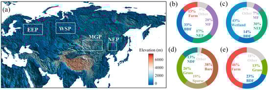
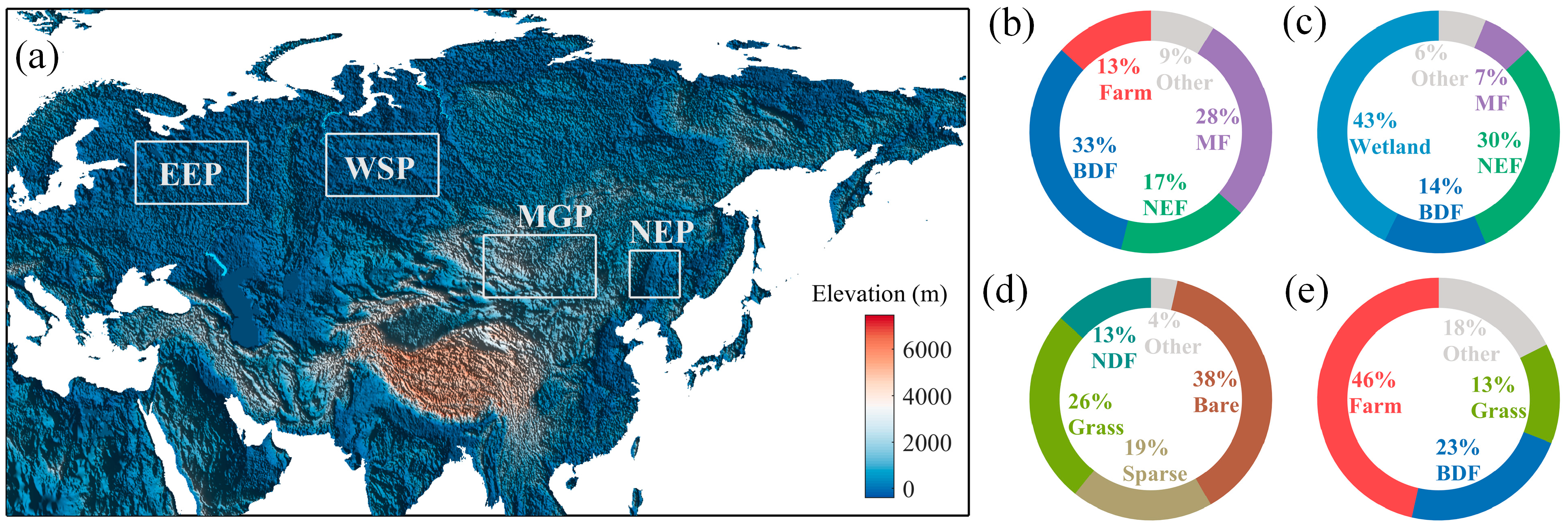
Figure 1.
Study area. (a) is the elevation map of the four typical regions in Eurasia, (b–e) represent the percentage of different ecosystems of EEP, WSP, MGP, and NEP, respectively, where the gray color represents other ecosystems with less area, which are not considered in this study.
The main ecosystem types in the EEP are farm (13%), deciduous broadleaf forest (BDF, 33%), evergreen needle leaved forest (NEF, 17%), and mixed forest (MF, 28%) (Figure 1b). WSP has the same forest type as EEP, but the largest ecosystem type in WSP is wetland (43%) (Figure 1c). MGP has an arid climate and the dominant vegetation types are the deciduous needle leaved forest (NDF, 13%), grass (26%), and sparse vegetation (Sparse, 19%), while the bare ground (Bare, 38%) ecosystem also accounts for a considerably large proportion (Figure 1d). Due to its suitable climate, the NEP has a high proportion of farm ecosystems (46%), followed by deciduous broadleaf forests (23%) and grasslands (13%) (Figure 1e). Note that the farmland in this study excludes irrigated agriculture to eliminate the impact of irrigation management on the results. In general, the four regions are highly representative in terms of climate and vegetation types, which greatly enhances the richness of the study.
To emphasize the effect of vegetation on clouds, the study period is the northern hemisphere summer (June, July, and August, JJA) from 2001 to 2021, when vegetation grows luxuriantly.
2.2. Datasets
2.2.1. Land Cover and Vegetation Data
The Land cover classification gridded map (2020), derived from satellite observations, was used to classify pixels in the study area. This map includes 22 land cover classes, which are defined using the United Nations Food and Agriculture Organization’s Land Cover Classification System. It has a spatial resolution of 300 m, and can be obtained from Copernicus Climate Change Service Climate Data Store [28]. Leaf area index (LAI) is derived from the Global Land Surface Satellite (GLASS) LAI product (version 6), which is superior to the MODIS LAI and is widely used in vegetation-related studies [29,30,31]. This product can be downloaded from http://www.glass.umd.edu/Download.html (accessed on 1 September 2022), with a spatiotemporal resolution of 0.25° × 0.25° and monthly.
2.2.2. Environmental Conditions, Heat Fluxes, and Surface Properties Data
The fifth-generation reanalysis of the European Centre for Medium-Range Weather Forecasts (ERA5) covers the period from 1940 to the present. It uses the laws of physics to combine model data with observations into a globally complete and consistent dataset. Research shows that the total cloud cover (TCC) in the ERA5 reanalysis is highly correlated with MODIS data (R = 0.95) and outperforms other reanalysis data on a global scale [32,33]. In addition, the ERA5 reanalysis data captures the variation of surface air temperature at 2 m (T2M) and relative humidity (RH) well [34]. The surface sensible heat flux (SSH) and surface latent heat flux (SLH) are also significantly improved [35,36]. Overall, the ERA5 reanalysis is of high quality [37], and is now widely used in climate research. Therefore, the variables required for the study, including TCC, surface albedo (Albedo), T2M, RH, SSH, SLH, soil water content (SW), and forecast surface roughness (FSR), were taken from the ERA5 reanalysis dataset [38,39]. The spatial and temporal resolutions are 0.25° × 0.25° and monthly, respectively (see Supplementary Table S2 for details). Note that the ECMWF Integrated Forecasting System has a four-layer representation of soil: Layer 1: 0–7 cm, Layer 2: 7–28 cm, Layer 3: 28–100 cm, and Layer 4: 100–289 cm. We used SW in the soil layer 1 (0–7 cm, the surface is at 0 cm) here. All data were refined to a spatial resolution of 0.1° × 0.1° using the bilinear interpolation method, which is widely used in current studies [40,41].
2.2.3. Elevation Data
The elevation data are from the Geospatial Information Authority of Japan (https://globalmaps.github.io/el.html, accessed on 24 July 2022), with a spatial resolution of 30 arcsecs.
2.3. Methods
2.3.1. Regression Methods
To explore the linear trend of TCC and LAI during the study period, a one-dimensional regression equation was established with the time series “t” as the independent variable, as shown in Equation (1). Here, y is the monthly mean of TCC or LAI. As the study period is the summer of 2001–2021, which covers a total of 63 months, t is the natural time series from 1 to 63 (t = 1, 2, 3, …61, 62, 63), k is the coefficient of the regression equation that characterizes the linear trend of TCC or LAI [40,42], and b0 is a constant term that is ignored in this study.
Next, a novel linear statistical approach, namely a partial least squares regression (PLSR), is employed here to distinguish the separate effects of 8 factors (the LAI, T2M, RH, Albedo, FSR, SW, SSH, and SLH) on the TCC. The PLSR, which originated around 1975 [43], not only solves the problem of multicollinearity among independent variables, but also applies to scenarios where the number of independent variables is greater than the number of samples. In general, PLSR improves the shortcomings of traditional multiple regression methods. The statistics analysis results and conclusions are more reliable and holistic [44,45]. After decades of theoretical development, this approach has been widely applied in scientific research [46,47,48,49].
Before modeling with PLSR, the independent and dependent variables are first standardized to eliminate dimensional differences among variables and make data comparable [48], as shown in Equation (2). Here, is the standardized X, and and are the mean and standard deviation of X, respectively. For more detailed modeling algorithms, see Wold et al. [50] and Chao et al. [47].
Using the 63-month time series of the independent and dependent variables, we performed PLSR for each pixel in the study area.
2.3.2. The 10-Fold Cross-Validation
When performing partial least squares regression modeling, selecting the appropriate number of components is a critical step. Here, 10-fold cross validation, a widely used method [51,52], was adopted to determine the optimal number of components for the PLSR model. In this method, the data are randomly divided into 10 parts, with 9 parts used for modeling and one part for validation, and rotated until all the data have been tested. This process is repeated 10 times. Determining the optimal number of components through 10-fold cross validation is a scientific approach that effectively avoids overfitting during modeling. As a result, the estimated model error is not optimistically biased.
2.3.3. The Relative Contribution of Each Factor to TCC
Referring to the previous studies [40,53], the relative contribution of each factor to the variation of TCC was further quantified based on the standard regression coefficient () from the optimal PLSR model, as shown in Equation (3). Here, represents the contribution of factor i to TCC, represents the absolute value of the standard regression coefficient of factor i, and represents the sum of the absolute values of the standard regression coefficients of 8 independent variables. Note that this relative contribution does not reflect a facilitative or inhibitory effect, but it still characterizes the relative importance of the factor to TCC.
2.3.4. K-Means Clustering
In the case study, to investigate how vegetation moderates the contribution of other factors to clouds, and to avoid the influence of non-local variables as much as possible, the pixels in the study area were clustered according to T2M and RH. The k-means clustering method, which is a widely used unsupervised learning algorithm [54,55], is adopted here. This method divides the samples into k clusters by maximizing the similarity between the same cluster and the difference among k clusters, and the specific algorithm can be found in Refs. [56,57]. The k-means clustering in this paper is performed using MATLAB (version 2023b). To guarantee the sample size of each category and not to complicate the issue, pixels were divided into 3 climate categories.
2.3.5. The Influence of LAI on the Factor Contribution
When exploring the influence of LAI on the factor’s contribution, the sample is simplified to avoid the interference of outliers. According to the ascending order of LAI, the pixels of each climate category are divided into N groups on average, and the LAI mean and the factor contribution mean of each group are calculated. Finally, the correlation analysis of the mean sequence is performed. The formula is as follows:
3. Results and Discussion
3.1. Temporal—Spatial Variations of TCC and LAI
Figure 2a–d show the spatial distribution of the multi-year mean of TCC (JJA). During the growing season, WSP and EEP have the highest TCC, with regional means of 0.64 and 0.61, respectively, followed by NEP (0.59), and MGP has the lowest TCC (0.53). The TCC distribution of EEP, WSP, and MGP shows the spatial pattern of high in the north and low in the south. The north–south variation of TCC is most obvious in MGP, with the main land type in the southern low TCC area being bare land, and the northern high TCC area coinciding well with the distribution of deciduous coniferous forests (Supplementary Figure S4c). In NEP, the areas with high TCC are distributed in the northwest, northeast, and southeast corners, and the vegetation is mainly deciduous broadleaf forest (Supplementary Figure S4d).
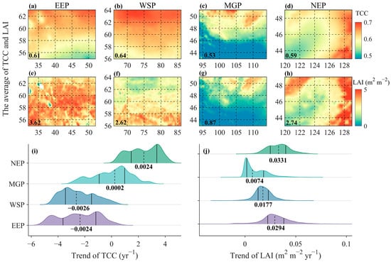
Figure 2.
Spatial and temporal variation of TCC and LAI from 2001–2021 (JJA). Where (a–h) are the spatial distributions of the multi-year mean (JJA) of TCC and LAI, respectively, with black numbers representing the mean of the corresponding region. Columns 1–4 represent EEP, WSP, MGP, and NEP, respectively. (i,j) are ridge plots characterizing the trend distributions of TCC and LAI (JJA), respectively, where the black dashed lines and numbers represent the median of the trends and the black solid lines represent the 25% and 75% quantiles of the trend, respectively.
From 2001 to 2021, EEP and WSP showed a pattern of decreasing TCC in almost the entire region, and the median of TCC trend was −0.0024 month−1 and −0.0026 month−1, respectively (Figure 2i). The MGP showed a pattern of increasing TCC in most areas, but decreased in the northwest and southeast (Supplementary Figure S5), with a median trend of 0.0002 month−1. TCC increased over almost the entire NEP, with the median of trend being 0.0024 month−1.
Figure 2e–h show the spatial distribution of LAI during the growing season. With respect to the regional mean, EEP is the region with the densest vegetation, with a mean LAI of 3.62 m2 m−2, and NEP (2.74 m2 m−2) and WSP (2.62 m2 m−2) are close to each other. Statistics on LAI trends indicate that vegetation greening has been occurring in recent years in our study area (Figure 2j). By comparing the median of LAI trends, it was found that vegetation greening in NEP was the fastest (0.0331 m2 m−2 month−1), followed by EEP (0.0294 m2 m−2 month−1). WSP was also obvious (0.0177 m2 m−2 month−1), and MGP was the slowest (0.0074 m2 m−2 month−1) due to large bare land occupation (Supplementary Figure S4c). Interestingly, in MGP and NEP, the area with high TCC is consistent with the area with high LAI to a great degree, but this feature is not found in the EEP and WSP, and even the area with high TCC in WSP corresponds to the area with low LAI.
In summary, there has been significant greening in the four regions. At the same time, the TCC of MGP and NEP increased significantly, while the TCC of EEP and WSP decreased.
3.2. The Relative Contribution of Different Factors to TCC
This study focuses on vegetation impacts on TCC, and thus vegetation and related factors including the LAI, surface air temperature at 2 m (T2M), relative humidity (RH), surface albedo (Albedo), forecast surface roughness (FSR), soil water content (SW: 0–7 cm, the surface is at 0 cm), surface sensible heat (SSH), and surface latent heat (SLH) are considered. The interdependencies among these variables are shown in Supplementary Figure S6. To compare the independent influence of the eight factors on TCC, we calculated their relative contribution based on the partial least squares regression (PLSR) method for each pixel. The contribution of all pixels in the same ecosystem was then averaged, as shown in Figure 3. The R2 of PLSR models indicate that the most cloud variability can be explained by vegetation (LAI), surface properties (Albedo, FSR, SW), environmental conditions (T2M, RH), and heat fluxes (SSH, SLH) (refer to Supplementary Figure S7 for details). More accurately, “relative contribution” refers to the relative magnitude of each factor’s influence in this explainable variation. In addition, Supplementary Figure S6 indicates that the relative contributions of the surface properties, environmental conditions, and heat fluxes actually include the indirect influence of LAI on TCC.
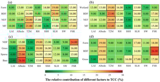
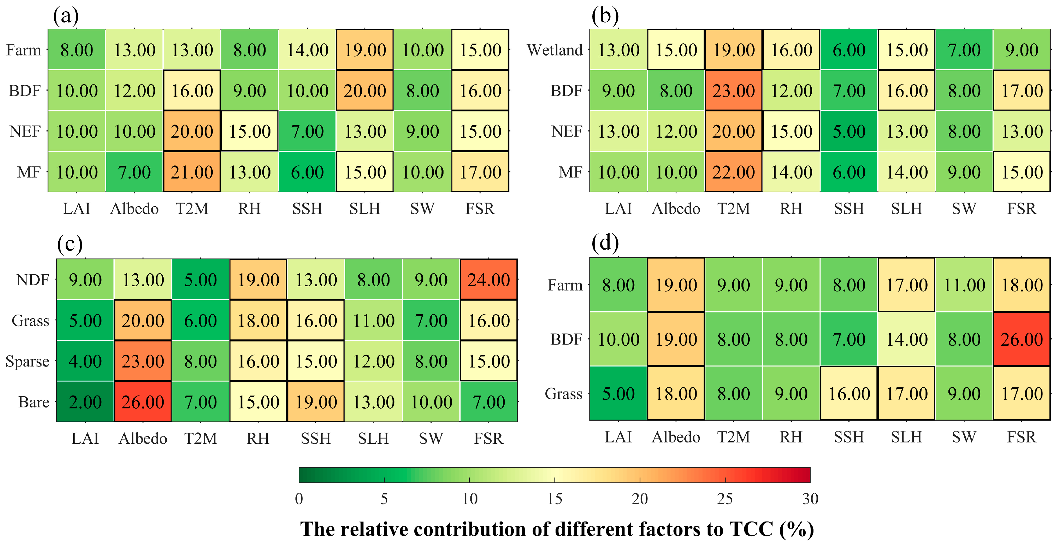
Figure 3.
The averaged relative contribution of the leaf area index (LAI), surface albedo (Albedo), surface air temperature at 2 m (T2M), relative humidity (RH), surface sensible heat flux (SSH), surface latent heat flux (SLH), soil water content (SW), and forecast surface roughness (FSR) to total cloud cover (TCC), where (a–d) represent EEP, WSP, MGP, and NEP, respectively. The numbers represent the percentage of the relative contribution. Note that when the averaged relative contribution exceeds 15%, it is highlighted with a black outline.
3.2.1. The Relative Contribution of LAI and Heat Fluxes
Generally, the contribution of LAI to TCC is relatively stable. In forests and farmland with high LAI, the relative contribution of LAI to TCC ranges from 8–13%. However, in grass and other ecosystems with low LAI, the relative contribution of LAI to TCC is relatively low. Note that in the WSP, the LAI of the wetland ecosystem is lower than that of the forest ecosystems (Supplementary Figure S9b), but its relative contribution to TCC is even higher (13%). The leaf surfaces of wetland plants contain more stomata and a thinner wax layer than those of terrestrial plants [58]. These leaf characteristics, combined with adequate soil moisture (Supplementary Figure S9j), allow the wetland plants to transfer water from the soil to the atmosphere more efficiently. Therefore, although the LAI of the wetland ecosystem is slightly lower, it still maintains a significant contribution to TCC.
In MGP, the SSH contributes more to TCC than SLH, which is opposite to the other three regions (Figure 3). This difference may be related to the energy allocation. Since the soil moisture in MGP is lower than those in other regions (Supplementary Figure S10j), the water sources available for evaporation are limited. In addition, the vegetation in the MGP is sparse and the LAI is very low (Supplementary Figure S10b), indicating that the transfer of water from the soil to the atmosphere by transpiration is inefficient. In short, although the atmospheric evaporation demand of the MGP is high, the arid climate condition and vegetation characteristics result in the weak ability of the region to meet the atmospheric evaporative demand. Research has shown that when evaporation is limited, SSH is the preferred way of heat conversion [59], which means that more heat is converted to SSH in MGP (Supplementary Figure S12c). This explains why the contribution of SSH is higher than that of SLH in MGP. Here, low LAI is one of the main reasons for limiting SLH, reflecting the indirect effect of LAI on TCC.
3.2.2. The Relative Contribution of Environmental Conditions
In EEP and WSP, T2M (13–23%) and RH (8–16%) both contribute greatly to TCC (Figure 3a,b). In contrast, the contributions of T2M and RH to TCC are all less than 10% in NEP (Figure 3d). For MGP, T2M has a small contribution to TCC (5–8%), while RH has a remarkable contribution to TCC (15–19%) (Figure 3c). This phenomenon is related to the environmental conditions of the regions themselves.
EEP and WSP are located at high latitudes in the northern hemisphere and border the Arctic Ocean, which results in low T2M and high RH in summer (Supplementary Figure S12a). The combination of T2M and RH indicates that EEP and WSP are more energy-limited rather than moisture-limited, resulting in the weak atmospheric evaporative demand. As T2M increases, the saturation water vapor pressure increases, leading to a decrease in RH [60]. The higher T2M and lower RH enhance the evaporative demand of the atmosphere, which facilitates the ecosystems to provide more water vapor for cloud formation through evapotranspiration. At the same time, the rising T2M may destabilize the lower atmosphere and cause a convective motion. If there is enough moisture in the lower atmosphere, the likelihood of cloud formation increases. The temperature perturbation and the resulting changes in RH can affect the thermodynamic conditions of cloud formation; thus, their contribution is higher in EEP and WSP. Note that the contribution of RH is slightly lower in EEP’s farm and BDF ecosystems, and the exact reason needs to be further investigated.
Both MGP and NEP are located in temperate regions, with higher T2M. NEP is close to the ocean, while MGP is inland. As a result, NEP has a high RH and MGP has a low RH (Supplementary Figure S12a). For the NEP with sufficient energy and moisture, the cloud cover is more limited by other factors, i.e., the variability of T2M and RH has less influence on the TCC, and their relative contributions are lower. For MGP, a more moisture-limited area, changing the RH constraint could have a significant effect on TCC.
In summary, in energy-limited (moisture-limited) areas, T2M (RH) is more likely to be the factor that contributes strongly to TCC, while in areas with adequate energy and moisture, TCC responds weakly to variations in T2M and RH.
3.2.3. The Relative Contribution of Surface Properties
FSR contributes greatly (13–26%) to TCC, except for the bare ecosystem in MGP and the wetland ecosystem in WSP. High surface roughness not only divides more solar radiation into turbulent heat fluxes, which enhances turbulent mixing and boundary layer instability [3], but also reduces the resistance to sensible heat and latent heat transport between the surface and the atmosphere [61], which promotes cloud formation. Comparing the four ecosystems of MGP, it was found that the FSR and its contribution to TCC decreased obviously as the vegetation cover decreased, proving that the change in surface roughness is one of the important ways that vegetation affects clouds formation.
In contrast to FSR, the contribution of albedo to TCC varies regionally: it is high in MGP and NEP, and low in EEP and WSP. The sparse vegetation of the MGP has a weak shading ability to the surface, and more dry soil is exposed, resulting in a bright surface. Similarly, 59% of the NEP was covered by farm and grass ecosystems (Figure 1e), which are lighter in color than the forests in EEP and WSP, i.e., the NEP also has a bright surface. The albedo of the bright surface is higher than that of the dark surface, so MGP and NEP have a higher albedo (Supplementary Figure S12b). The high albedo reduces the net surface radiation, which changes the temperature difference between the near-surface and upper atmosphere, weakening the thermal conditions for cloud formation. Therefore, the influence of albedo on TCC is greater in MGP and NEP.
Compared with the albedo and FSR, the contribution of SW (0–7 cm, the surface is at 0 cm) to TCC is more stable and does not vary much among different ecosystems (7–11%). In areas that are not extremely wet, evaporation is regulated by the availability of SW [62]. As transpiration and soil evaporation transfer SW to the atmosphere, the upper soil becomes drier, which directly limits soil evaporation. For shallow-rooted vegetation like grass, when the SW is below the vegetation wilting point, the soil water cannot enter the plant roots, the transpiration is weakened, and more energy is converted to SSH [63]. Deep-rooted vegetation such as forests can only maintain transpiration by accessing deeper soil water. As a result, the water supplied by upper soil (0–7 cm, the surface is at 0 cm) to cloud formation via ET gradually decreases or even stops, which explains why the contribution of SW to clouds is stable and limited.
3.3. The Regulatory Role of Vegetation
Based on the factor contributions obtained using PLSR, this subsection further discusses how vegetation moderates the contribution of other factors to TCC using all spatial pixels as samples. The farmland (2578 pixels) of NEP and the BDF (5349 pixels) of EEP were selected for this case study, since NEP and EEP have more pronounced vegetation greening (Figure 2j), and the two ecosystems have the largest area relative to other ecosystems.
The contribution of each factor to the TCC is influenced by both vegetation and non-local variables (moisture and heat advection, atmospheric circulation). To investigate the moderating effect of vegetation on the factor contributions, it is necessary to control the influence of non-local variables. Based on k-means clustering, the pixels are clustered into three climate categories according to T2M and RH, as shown in Figure 4b,d. After clustering, the pixels within the same category have more similar climatic backgrounds, then the influence of non-local variables on factor contributions are approximated, and the differences in factor contributions among different pixels are mainly caused by vegetation. Then, the correlation analysis between vegetation and factor contributions can easily reveal the direction of vegetation regulation of factor contributions.
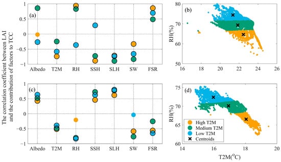
Figure 4.
The correlation coefficient between LAI and the contribution of other factors to TCC, where (a,c) represent the farm and BDF ecosystems, respectively. The black circle indicates p < 0.1, and (b,d) are the clustering results of the farmland and BDF based on the K-means clustering method. The black × marks centroids of the three clusters. Note the full names of these abbreviations: LAI (leaf area index), Albedo (surface albedo), T2M (surface air temperature at 2 m), RH (relative humidity), SSH (surface sensible heat flux), SLH (surface latent heat flux), SW (soil water content), and FSR (forecast surface roughness).
Note that the sample of each climate category was simplified to 60 groups before the correlation analysis was conducted, as described in Methods, and the results are shown in Figure 4a,c.
For convenience, the relative contribution of environmental conditions, surface properties, and heat fluxes to TCC will be abbreviated as Cenvironment, Csurface, and Cheat, respectively.
3.3.1. The Regulation of Vegetation to Cenvironment
In farm and BDF ecosystems, the contribution of T2M to clouds is significantly (p < 0.1) negatively correlated with LAI. This is because the increasing LAI leads to a decrease in T2M (Supplementary Figure S13), which weakens the temperature difference between near-surface and upper atmosphere, and is not conducive to upward motion and cloud formation.
High LAI not only attenuates saturated water vapor pressure by affecting T2M, but also releases more water vapor into the atmosphere through transpiration, which helps to increase RH (Supplementary Figure S13). A high RH indicates that there is sufficient water vapor in the air, which is an important guarantee for cloud formation. Thus, the contribution of RH to TCC increases with LAI, as shown by the yellow and green dots in Figure 4a. Interestingly, in the low-temperature farmland (blue dots) and BDF ecosystems, the contribution of RH shows the opposite. This is because the farm (blue dots) and BDF ecosystems are originally located in areas with high RH, as the increase in LAI and water vapor is no longer a limiting condition for cloud development, so the relative contribution of RH to TCC naturally decreases.
3.3.2. The Regulation of Vegetation to Csurface
With increasing LAI, the relative contribution of albedo to TCC increases in both regions except for the low temperature farmland (blue dots), but the direction of the contribution is the opposite. The decrease in albedo in farm ecosystem favors the increase in TCC, while the increase in albedo in BDF ecosystem is detrimental to cloud formation (Supplementary Figure S13). Increasing LAI enhances the interception of radiation reaching the surface, which is not conducive to soil evapotranspiration [64,65]. Additionally, the growth of vegetation and the process of evapotranspiration can cause the upper layers of soil to become dry. Thus, the relative contribution of SW (0–7 cm, the surface is at 0 cm) to TCC decreases.
In farmland, the contribution of FSR to TCC increases significantly with LAI (p < 0.1) (Figure 4a). This is because FSR effectively reduces the resistance to sensible heat and latent heat transport between the surface and the atmosphere [61]. The FSR of the BDF is high, and the change in FSR induced by LAI is weak. In this case, the changes in other factors caused by LAI may gradually play a more important role in the variation of TCC, and then the relative contribution of FSR decreases with the increase of LAI.
3.3.3. The Regulation of Vegetation to Cheat
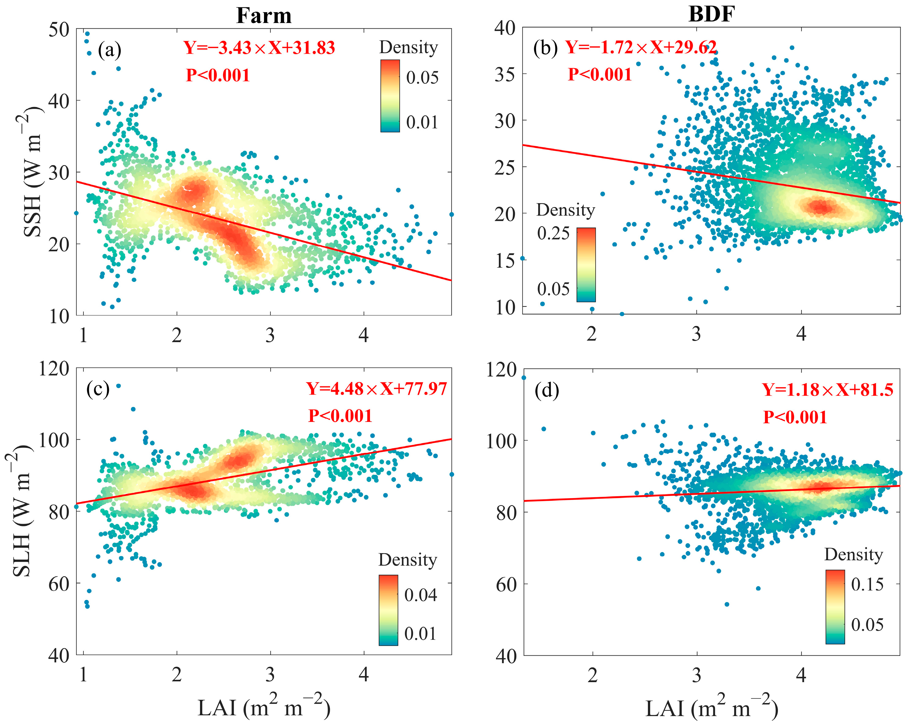
As LAI increases, the direction of energy allocation is essentially the same for both ecosystem types: lower SSH, and higher SLH. However, the relative contribution of SSH and SLH to TCC decreases in the farm ecosystem (excluding blue dots) and increases in the BDF (Figure 4). This may be related to the rate at which heat fluxes respond to LAI.
Previous studies have demonstrated that high moisture content at the surface helps to reduce lifting condensation height (LCH) [66,67]. Our study also found a similar phenomenon: LAI leads to an increase in surface RH (Supplementary Figure S14a,b), which reduces the lifting condensation height (Supplementary Figure S14c,d). As the lifting condensation height decreases, cloud formation has lower requirements for thermal conditions. However, the SSH in the farm ecosystem decreases dramatically with the increasing LAI (Figure 5a), which means that the thermal uplift can only lift the bottom air mass to a lower altitude, where only a few air masses with high RH can reach the LCH. Therefore, the sharp decline in SSH results in fewer air masses having the opportunity to form clouds. Naturally, the contribution of SSH and SLH to the TCC decreases with the increasing LAI.
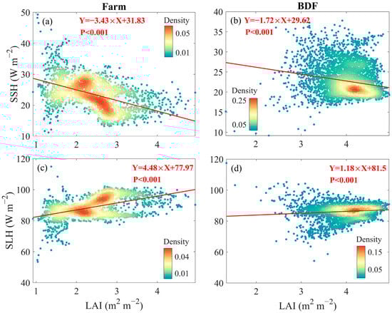
Figure 5.
The changes in heat fluxes with LAI, where (a,b) are SSH of the farm and BDF ecosystems, while (c,d) are SLH.
In BDF, SSH decreased slowly with LAI (Figure 5c), accompanied by the decrease in LCH, and more air masses can reach LCH and form clouds, i.e., the changes in SSH and SLH increased the probability of lower air masses to form clouds, and their contributions to TCC were positively correlated with LAI. The above suggests that vegetation has a complex influence on TCC by affecting energy allocation, and there may be constraints on the contribution of different factors to TCC, such as the constraints of SSH on SLH.
Note that the variation of Cheat with LAI in low-temperature farmland (blue dots) differs somewhat from the above, which is again related to energy partitioning. Supplementary Figure S15 shows that SSH increases with LAI in farms with low temperatures, while SLH decreases. In conditions of low T2M and high RH, moisture is not the primary limiting factor for cloud formation; rather, energy that uplifts cloud upward motion is more important. Therefore, as the LAI increases, the relative contribution of SSH increases while SLH decreases. The allocation of energy in low-temperature farmland is unique, and can be influenced by various reasons, such as the type of crops. However, this study will not delve into these specific reasons.
3.4. A New Idea for Slowing Global Warming
Our study of typical vegetation regions in Eurasia demonstrates that vegetation has a significant impact on TCC. Previous studies have shown that changes in clouds affect the albedo at the top of the atmosphere (TOA), which alters the radiative balance of the earth–atmosphere system [68,69]. Based on this, we present the idea of using vegetation impacts on clouds to enhance albedo at the TOA and ultimately decrease incident radiation, partially offsetting the warming effects of heightened CO2 concentration. This idea aligns with the existing widely supported idea of solar geoengineering [70]. The sixth report of the Intergovernmental Panel on Climate Change (IPCC) states that the sudden cessation of solar geoengineering could result in swift climate change [71]. However, this problem does not arise when vegetation is used to indirectly intervene with radiation, as it can grow sustainably and influence cloud cover, unless the environment is unfavorable or anthropogenic.
Can a comprehensive inventory of vegetation types be developed that maximizes the contribution of vegetation in mitigating global warming, considering their photosynthetic carbon sequestration and intervention of incident solar radiation (through changing TCC)? This idea requires more complex work to refine the theory, as well as combining observations and Earth system models (ESMs). First, more vegetation properties should be considered, such as the oxidation of volatile organic compounds released by vegetation, which can act as cloud condensation nuclei. Second, whether the overall effect of vegetation on cloudiness is an increase or decrease must be determined. In addition, the influence of vegetation on cloud types deserves an in-depth and comprehensive study, as there may be differences in the feedback of different cloud types to radiation [69]. In conclusion, the full utilization of vegetation’s influence on clouds may aid humans in slowing global warming, an avenue worth exploring.
3.5. Limitations and Future Perspectives
Our results highlight the important influence of vegetation on TCC and emphasize the differences between various vegetation types. Also, we acknowledge the uncertainties and limitations of this study.
The gridded data of ERA5 has advantages over direct station observations and satellite remote sensing data, which is one of the main reasons for our choice. However, most of the variables come from ERA5 reanalysis, which means that they have undergone the same assimilation process, potentially leading to internal consistency among these variables. This consistency may lead to optimistic estimates in the partial least squares regression model. In addition, the relationships among these variables are somewhat dependent on the Integrated Forecasting System of ERA5. In future research, it is advisable to include multi-source datasets to ensure the generalizability of the model and the robustness of the results. Note that the cluster analysis cannot entirely eliminate the influence of non-local variables. Additionally, when calculating the forcing using monthly average data (a mixture of “slow” and “fast” forcing), contemporaneous analysis ignores the fact that the temporal variability of “slow” phenomena, such as vegetation, is slower than that of “fast” atmospheric phenomena, such as cloud cover. Therefore, this paper quantifies the limited feedback (spatially local and temporally “fast”). Finally, our methods do not effectively isolate the TCC forcing on vegetation and surface variables, leading to some uncertainty in the findings as well. To address these limitations, it is essential to improve the methodology and conduct more in-depth analyses.
4. Conclusions
Based on GLASS LAI products and ERA5 reanalysis datasets, this study investigates the spatial and temporal heterogeneity of TCC in typical ecosystems in the northern growing season, then quantified the relative contribution of different factors to TCC using the PLSR method, and finally explored how vegetation modulated the contribution of other factors to TCC. The main findings are as follows:
- (1)
- During 2001–2021, TCC decreased in EEP (−0.0024 month−1) and WSP (−0.0026 month−1), while it increased in MGP (0.0002 month−1) and NCP (0.0024 month−1).
- (2)
- The relative contribution of different factors to TCC was closely related to the climate and vegetation characteristics. In energy-limited (moisture-limited) areas, temperature (relative humidity) was more likely to be the factor that strongly contributed to TCC variation. In terms of energy allocation, the dry MGP tended to convert more heat into SSH rather than SLH to promote cloud formation. The contribution of LAI to TCC was higher in forest ecosystems due to the high LAI.
- (3)
- The case study shows that the contribution of other factors to TCC changed significantly with the increasing LAI, i.e., vegetation significantly regulated the contribution of other factors to TCC, but this regulation varied among ecosystems.
Overall, this study explored the vegetation impacts on TCC in a greening world and compared the differences among ecosystems, which helps to understand the feedback of vegetation on climate and provides some guidance for improving the earth system models.
Supplementary Materials
The following supporting information can be downloaded at: https://www.mdpi.com/article/10.3390/rs16122048/s1, Figure S1: The wind direction map of the study area in 2001 (JJA); Figure S2: The wind direction map of the study area in 2010 (JJA); Figure S3: The wind direction map of the study area in 2021 (JJA); Figure S4: Distribution of main ecosystem types in the EEP, WSP MGP and NEP; Figure S5: The spatial distribution of TCC and LAI trends from 2001 to 2021(JJA); Figure S6: The interdependency among LAI, surface properties (Albedo, FSR and SW), environmental conditions (T2M and RH) and heat fluxes (SSH and SLH) under greening background; Figure S7: The R2 of partial least squares regression models; Figure S8: Box plots of different factors in EEP (JJA); Figure S9: Box plots of different factors in WSP (JJA); Figure S10: Box plots of different factors in MGP (JJA); Figure S11: Box plots of different factors in NEP (JJA); Figure S12: Multi-year summer averages of (a) environmental conditions, (b) surface properties, and (c) heat fluxes in four regions; Figure S13: Pearson correlation coefficients between LAI and other factors; Figure S14: Scatter plots of relative humidity (RH) and lifting condensation height (LCH) as a function of leaf area index (LAI); Figure S15: The changes in (a) SSH and (b) SLH with LAI in low temperature farmland (NEP); Figure S16: Multicollinearity diagnostic results for four regions; Figure S17: The trend distributions of TCC and LAI (JJA); Figure S18: The spatial distribution of TCC and LAI trend from 2001 to 2021(JJA); Table S1: Range and elevation information for 4 regions; Table S2: Details of datasets used in this study; Table S3: Abbreviation of terms [72,73,74,75,76,77].
Author Contributions
Conceptualization, Y.H.; methodology, T.L. and Y.H.; software, T.L. and Y.H.; validation, T.L. and Y.H.; formal analysis, T.L.; investigation, T.L., Y.H., Q.Z., L.D., Y.Z., X.D. and D.X.; resources, T.L.; data curation, T.L.; writing—original draft preparation, T.L.; writing—review and editing, T.L. and Y.H.; visualization, T.L.; supervision, Y.H.; project administration, Y.H.; funding acquisition, Y.H. All authors have read and agreed to the published version of the manuscript.
Funding
This research was funded by the National Natural Science Foundation of China (grant Nos. 42027804, 41775026, and 41075012).
Data Availability Statement
The Land cover classification gridded map (2020) derived from satellite observations is available at Land cover classification gridded maps from 1992 to present derived from satellite observations (https://cds.climate.copernicus.eu/cdsapp#!/dataset/satellite-land-cover?tab=overview, accessed on 4 July 2022). The elevation data comes from the Geospatial Information Authority of Japan are available at https://globalmaps.github.io/el.html (accessed on 24 July 2022). The GLASS LAI product can be found at http://www.glass.umd.edu/Download.html (accessed on 1 September 2022). The ERA5 reanalysis data can be accessed from https://www.ecmwf.int/en/forecasts/datasets (accessed on 4 August 2022).
Acknowledgments
The authors are very grateful to the two anonymous reviewers for their valuable comments, which significantly improved the quality of our paper and enhanced our understanding of the scientific issues of vegetation impacts on clouds.
Conflicts of Interest
The authors declare no conflict of interest.
References
- Bosman, P.J.M.; van Heerwaarden, C.C.; Teuling, A.J. Sensible Heating as a Potential Mechanism for Enhanced Cloud Formation over Temperate Forest. Q. J. R. Meteorol. Soc. 2019, 145, 450–468. [Google Scholar] [CrossRef]
- Cho, M.-H.; Yang, A.-R.; Baek, E.-H.; Kang, S.M.; Jeong, S.-J.; Kim, J.Y.; Kim, B.-M. Vegetation-Cloud Feedbacks to Future Vegetation Changes in the Arctic Regions. Clim. Dyn. 2018, 50, 3745–3755. [Google Scholar] [CrossRef]
- Xu, R.; Li, Y.; Teuling, A.J.; Zhao, L.; Spracklen, D.V.; Garcia-Carreras, L.; Meier, R.; Chen, L.; Zheng, Y.; Lin, H.; et al. Contrasting Impacts of Forests on Cloud Cover Based on Satellite Observations. Nat. Commun. 2022, 13, 670. [Google Scholar] [CrossRef]
- Piao, S.; Wang, X.; Park, T.; Chen, C.; Lian, X.; He, Y.; Bjerke, J.W.; Chen, A.; Ciais, P.; Tømmervik, H.; et al. Characteristics, Drivers and Feedbacks of Global Greening. Nat. Rev. Earth Environ. 2020, 1, 14–27. [Google Scholar] [CrossRef]
- Zeng, Z.; Piao, S.; Li, L.Z.X.; Wang, T.; Ciais, P.; Lian, X.; Yang, Y.; Mao, J.; Shi, X.; Myneni, R.B. Impact of Earth Greening on the Terrestrial Water Cycle. J. Clim. 2018, 31, 2633–2650. [Google Scholar] [CrossRef]
- Garcia-Carreras, L.; Marsham, J.H.; Spracklen, D.V. Observations of Increased Cloud Cover over Irrigated Agriculture in an Arid Environment. J. Hydrometeorol. 2017, 18, 2161–2172. [Google Scholar] [CrossRef]
- Laguë, M.M.; Swann, A.L.S. Progressive Midlatitude Afforestation: Impacts on Clouds, Global Energy Transport, and Precipitation. J. Clim. 2016, 29, 5561–5573. [Google Scholar] [CrossRef]
- Portmann, R.; Beyerle, U.; Davin, E.; Fischer, E.M.; De Hertog, S.; Schemm, S. Global Forestation and Deforestation Affect Remote Climate via Adjusted Atmosphere and Ocean Circulation. Nat. Commun. 2022, 13, 5569. [Google Scholar] [CrossRef] [PubMed]
- Sikma, M.; de Arellano, J.V.; Pedruzo-Bagazgoitia, X.; Voskamp, T.; Heusinkveld, B.; Anten, N.; Evers, J. Impact of Future Warming and Enhanced [CO2] on the Vegetation-Cloud Interaction. J. Geophys. Res. 2019, 124, 12444–12454. [Google Scholar] [CrossRef]
- Manoli, G.; Domec, J.-C.; Novick, K.A.; Oishi, A.C.; Noormets, A.; Marani, M.; Katul, G.G. Soil–Plant–Atmosphere Conditions Regulating Convective Cloud Formation above Southeastern US Pine Plantations. Glob. Chang. Biol. 2016, 22, 2238–2254. [Google Scholar] [CrossRef]
- Sakaguchi, K.; Berg, L.K.; Chen, J.; Fast, J.; Newsom, R.; Tai, S.-L.; Yang, Z.; Gustafson, W.I.; Gaudet, B.J.; Huang, M.; et al. Determining Spatial Scales of Soil Moisture—Cloud Coupling Pathways Using Semi-Idealized Simulations. J. Geophys. Res. Atmos. 2022, 127, e2021JD035282. [Google Scholar] [CrossRef]
- Taylor, C.M.; de Jeu, R.A.M.; Guichard, F.; Harris, P.P.; Dorigo, W.A. Afternoon Rain More Likely over Drier Soils. Nature 2012, 489, 423–426. [Google Scholar] [CrossRef] [PubMed]
- Jach, L.; Warrach-Sagi, K.; Ingwersen, J.; Kaas, E.; Wulfmeyer, V. Land Cover Impacts on Land-Atmosphere Coupling Strength in Climate Simulations with WRF Over Europe. J. Geophys. Res. Atmos. 2020, 125, e2019JD031989. [Google Scholar] [CrossRef]
- Bell, J.P.; Tompkins, A.M.; Bouka-Biona, C.; Sanda, I.S. A Process-based Investigation into the Impact of the Congo Basin Deforestation on Surface Climate. J. Geophys. Res. 2015, 120, 5721–5739. [Google Scholar] [CrossRef]
- Heinze, R.; Moseley, C.; Böske, L.N.; Muppa, S.K.; Maurer, V.; Raasch, S.; Stevens, B. Evaluation of Large-Eddy Simulations Forced with Mesoscale Model Output for a Multi-Week Period during a Measurement Campaign. Atmos. Chem. Phys. 2017, 17, 7083–7109. [Google Scholar] [CrossRef]
- Chagnon, F.J.F.; Bras, R.L.; Wang, J. Climatic Shift in Patterns of Shallow Clouds over the Amazon. Geophys. Res. Lett. 2004, 31, L24212. [Google Scholar] [CrossRef]
- Wang, J.; Chagnon, F.J.F.; Williams, E.; Betts, A.K.; Renno, N.O.; Machado, L.A.T.; Bisht, G.; Knox, R.G.; Bras, R.L. Impact of Deforestation in the Amazon Basin on Cloud Climatology. Proc. Natl. Acad. Sci. USA 2009, 106, 3670–3674. [Google Scholar] [CrossRef] [PubMed]
- Spracklen, D.V.; Bonn, B.; Carslaw, K.S. Boreal Forests, Aerosols and the Impacts on Clouds and Climate. Philos. Trans. R. Soc. A 2008, 366, 4613–4626. [Google Scholar] [CrossRef]
- Zhao, D.; Buchholz, A.; Tillmann, R.; Kleist, E.; Wu, C.; Rubach, F.; Kiendler-Scharr, A.; Rudich, Y.; Wildt, J.; Mentel, T.F. Environmental Conditions Regulate the Impact of Plants on Cloud Formation. Nat. Commun. 2017, 8, 14067. [Google Scholar] [CrossRef] [PubMed]
- Carleton, A.M.; Adegoke, J.; Allard, J.; Arnold, D.L.; Travis, D.J. Summer Season Land Cover—Convective Cloud Associations for the Midwest U.S. “Corn Belt”. Geophys. Res. Lett. 2001, 28, 1679–1682. [Google Scholar] [CrossRef]
- Li, Y.; Liu, Y.; Bohrer, G.; Cai, Y.; Wilson, A.; Hu, T.; Wang, Z.; Zhao, K. Impacts of Forest Loss on Local Climate across the Conterminous United States: Evidence from Satellite Time-Series Observations. Sci. Total Environ. 2021, 802, 149651. [Google Scholar] [CrossRef] [PubMed]
- O’neal, M. Interactions between Land Cover and Convective Cloud Cover over Midwestern North America Detected from GOES Satellite Data. Int. J. Remote Sens. 1996, 17, 1149–1181. [Google Scholar] [CrossRef]
- da Silva, H.J.F.; Gonçalves, W.A.; Bezerra, B.G.; Santos e Silva, C.M.; Oliveira, C.P.D.; Mutti, P.R. Cláudio Moisés Santos e Silva; Cristiano Prestrelo de Oliveira; Mutti, P.R. Analysis of the Influence of Deforestation on the Microphysical Parameters of Clouds in the Amazon. Remote Sens. 2022, 14, 5353. [Google Scholar] [CrossRef]
- Heiblum, R.H.; Koren, I.; Feingold, G. On the Link between Amazonian Forest Properties and Shallow Cumulus Cloud Fields. Atmos. Chem. Phys. 2014, 14, 6063–6074. [Google Scholar] [CrossRef]
- Pinto, E.; Shin, Y.; Cowling, S.A.; Jones, C.; Jones, C.D. Past, Present and Future Vegetation-Cloud Feedbacks in the Amazon Basin. Clim. Dyn. 2009, 32, 741–751. [Google Scholar] [CrossRef]
- Pauli, E.; Cermak, J.; Teuling, R.; Teuling, A.J. Enhanced Nighttime Fog and Low Stratus Occurrence over the Landes Forest, France. Geophys. Res. Lett. 2022, 49, e2021GL097058. [Google Scholar] [CrossRef]
- Teuling, A.J.; Taylor, C.M.; Meirink, J.F.; Melsen, L.A.; Miralles, D.G.; Van Heerwaarden, C.C.; Vautard, R.; Stegehuis, A.I.; Nabuurs, G.-J.; Vila-Guerau de Arellano, J. Observational Evidence for Cloud Cover Enhancement over Western European Forests. Nat. Commun. 2017, 8, 14065. [Google Scholar] [CrossRef] [PubMed]
- Copernicus Climate Change Service. Land Cover Classification Gridded Maps from 1992 to Present Derived from Satellite Observations. 2019. Available online: https://cds.climate.copernicus.eu/cdsapp#!/dataset/satellite-land-cover?tab=overview (accessed on 4 July 2022).
- Li, J.; Xiao, Z. Evaluation of the Version 5.0 Global Land Surface Satellite (GLASS) Leaf Area Index Product Derived from MODIS Data. Int. J. Remote Sens. 2020, 41, 9140–9160. [Google Scholar] [CrossRef]
- Xiang, Y.; Xiao, Z.Q.; Liang, S.; Wang, J.D.; Song, J.L. Validation of Global LAnd Surface Satellite (GLASS) Leaf Area Index Product. J. Remote Sens. 2014, 18, 573–596. [Google Scholar]
- Zhao, Y.; Feng, J.; Luo, L.; Bai, L.; Wan, H.; Ren, H. Monitoring Cropping Intensity Dynamics across the North China Plain from 1982 to 2018 Using GLASS LAI Products. Remote Sens. 2021, 13, 3911. [Google Scholar] [CrossRef]
- Wu, H.; Xu, X.; Luo, T.; Yang, Y.; Xiong, Z.; Wang, Y. Variation and Comparison of Cloud Cover in MODIS and Four Reanalysis Datasets of ERA-Interim, ERA5, MERRA-2 and NCEP. Atmos. Res. 2023, 281, 106477. [Google Scholar] [CrossRef]
- Yao, B.; Teng, S.; Lai, R.; Xu, X.; Yin, Y.; Shi, C.; Liu, C. Can Atmospheric Reanalyses (CRA and ERA5) Represent Cloud Spatiotemporal Characteristics? Atmos. Res. 2020, 244, 105091. [Google Scholar] [CrossRef]
- Dai, A. The Diurnal Cycle from Observations and ERA5 in Surface Pressure, Temperature, Humidity, and Winds. Clim. Dyn. 2023, 61, 2965–2990. [Google Scholar] [CrossRef]
- Martens, B.; Schumacher, D.L.; Wouters, H.; Muñoz-Sabater, J.; Verhoest, N.E.C.; Miralles, D.G. Evaluating the Land-Surface Energy Partitioning in ERA5. Geosci. Model Dev. 2020, 13, 4159–4181. [Google Scholar] [CrossRef]
- Xin, Y.; Liu, J.; Liu, X.; Liu, G.; Cheng, X.; Chen, Y. Reduction of Uncertainties in Surface Heat Flux over the Tibetan Plateau from ERA-Interim to ERA5. Int. J. Climatol. 2022, 42, 6277–6292. [Google Scholar] [CrossRef]
- Hersbach, H.; Bell, B.; Berrisford, P.; Hirahara, S.; Horányi, A.; Muñoz-Sabater, J.; Nicolas, J.; Peubey, C.; Radu, R.; Schepers, D.; et al. The ERA5 Global Reanalysis. Q. J. R. Meteorol. Soc. 2020, 146, 1999–2049. [Google Scholar] [CrossRef]
- Hersbach, H.; Bell, B.; Berrisford, P.; Biavati, G.; Horányi, A.; Muñoz Sabater, J.; Nicolas, J.; Peubey, C.; Radu, R.; Rozum, I.; et al. ERA5 Monthly Averaged Data on Single Levels from 1940 to Present. 2023. Available online: https://cds.climate.copernicus.eu/cdsapp#!/dataset/10.24381/cds.f17050d7?tab=overview (accessed on 4 August 2022).
- Hersbach, H.; Bell, B.; Berrisford, P.; Biavati, G.; Horányi, A.; Muñoz Sabater, J.; Nicolas, J.; Peubey, C.; Radu, R.; Rozum, I.; et al. ERA5 Monthly Averaged Data on Pressure Levels from 1940 to Present. 2023. Available online: https://cds.climate.copernicus.eu/cdsapp#!/dataset/10.24381/cds.6860a573?tab=overview (accessed on 4 August 2022).
- Lu, T.; Han, Y.; Dong, L.; Zhang, Y.; Zhu, X.; Xu, D. Evapotranspiration Responses to CO2 and Its Driving Mechanisms in Four Ecosystems Based on CMIP6 Simulations: Forest, Shrub, Farm and Grass. Environ. Res. 2023, 223, 115417. [Google Scholar] [CrossRef]
- Wei, J.; Li, Z.; Li, K.; Dickerson, R.R.; Pinker, R.T.; Wang, J.; Liu, X.; Sun, L.; Xue, W.; Cribb, M. Full-Coverage Mapping and Spatiotemporal Variations of Ground-Level Ozone (O3) Pollution from 2013 to 2020 across China. Remote Sens. Environ. 2022, 270, 112775. [Google Scholar] [CrossRef]
- He, Q.; Zhang, M.; Huang, B. Spatio-Temporal Variation and Impact Factors Analysis of Satellite-Based Aerosol Optical Depth over China from 2002 to 2015. Atmos. Environ. 2016, 129, 79–90. [Google Scholar] [CrossRef]
- Wold, H. Soft modeling: The basic design and some extensions. In Systems under Indirect Observations: Part II; Joreskog, K.G., Wold, H., Eds.; North-Holland: Amsterdam, The Netherlands, 1982; pp. 1–54. [Google Scholar]
- Li, Q. Statistical Modeling Experiment of Land Precipitation Variations since the Start of the 20th Century with External Forcing Factors. Chin. Sci. Bull. 2020, 65, 2266–2278. [Google Scholar] [CrossRef]
- Yang, Y.; Wu, Z.; Guo, L.; He, H.S.; Ling, Y.; Wang, L.; Zong, S.; Na, R.; Du, H.; Li, M.-H. Effects of Winter Chilling vs. Spring Forcing on the Spring Phenology of Trees in a Cold Region and a Warmer Reference Region. Sci. Total Environ. 2020, 725, 138323. [Google Scholar] [CrossRef] [PubMed]
- Cao, R.; Shen, M.; Zhou, J.; Chen, J. Modeling Vegetation Green-up Dates across the Tibetan Plateau by Including Both Seasonal and Daily Temperature and Precipitation. Agric. For. Meteorol. 2018, 249, 176–186. [Google Scholar] [CrossRef]
- Chao, L.; Li, Q.; Dong, W.; Yang, Y.; Guo, Z.; Huang, B.; Zhou, L.; Jiang, Z.; Zhai, P.; Jones, P. Vegetation Greening Offsets Urbanization-Induced Fast Warming in Guangdong, Hong Kong, and Macao Region (GHMR). Geophys. Res. Lett. 2021, 48, e2021GL095217. [Google Scholar] [CrossRef]
- Chen, C.; He, B.; Guo, L.; Zhang, Y.; Xie, X.; Chen, Z. Identifying Critical Climate Periods for Vegetation Growth in the Northern Hemisphere. J. Geophys. Res. Biogeosci. 2018, 123, 2541–2552. [Google Scholar] [CrossRef]
- Emerson, J.B.; Varner, R.K.; Wik, M.; Parks, D.H.; Neumann, R.B.; Johnson, J.E.; Singleton, C.M.; Woodcroft, B.J.; Tollerson, R.; Owusu-Dommey, A.; et al. Diverse Sediment Microbiota Shape Methane Emission Temperature Sensitivity in Arctic Lakes. Nat. Commun. 2021, 12, 5815. [Google Scholar] [CrossRef] [PubMed]
- Wold, S.; Sjöström, M.; Eriksson, L. PLS-Regression: A Basic Tool of Chemometrics. Chemom. Intell. Lab. Syst. 2001, 58, 109–130. [Google Scholar] [CrossRef]
- Wei, J.; Li, Z.; Cribb, M.; Huang, W.; Xue, W.; Sun, L.; Guo, J.; Peng, Y.; Li, J.; Lyapustin, A.; et al. Improved 1 Km Resolution PM2.5 Estimates across China Using Enhanced Space–Time Extremely Randomized Trees. Atmos. Chem. Phys. 2020, 20, 3273–3289. [Google Scholar] [CrossRef]
- Xue, W.; Wei, J.; Zhang, J.; Sun, L.; Che, Y.; Yuan, M.; Hu, X. Inferring Near-Surface PM2.5 Concentrations from the VIIRS Deep Blue Aerosol Product in China: A Spatiotemporally Weighted Random Forest Model. Remote Sens. 2021, 13, 505. [Google Scholar] [CrossRef]
- Fu, J.; Gong, Y.; Zheng, W.; Zou, J.; Zhang, M.; Zhang, Z.; Qin, J.; Liu, J.; Quan, B. Spatial-Temporal Variations of Terrestrial Evapotranspiration across China from 2000 to 2019. Sci. Total Environ. 2022, 825, 153951. [Google Scholar] [CrossRef] [PubMed]
- Zeraatpisheh, M.; Ayoubi, S.; Brungard, C.W.; Finke, P. Disaggregating and Updating a Legacy Soil Map Using DSMART, Fuzzy c-Means and k-Means Clustering Algorithms in Central Iran. Geoderma 2019, 340, 249–258. [Google Scholar] [CrossRef]
- Zhao, W.; Ma, J.; Liu, Q.; Song, J.; Tysklind, M.; Liu, C.; Wang, D.; Qu, Y.; Wu, Y.; Wu, F. Comparison and Application of SOFM, Fuzzy c-Means and k-Means Clustering Algorithms for Natural Soil Environment Regionalization in China. Environ. Res. 2023, 216, 114519. [Google Scholar] [CrossRef] [PubMed]
- Borge, R.; Jung, D.; Lejarraga, I.; de la Paz, D.; Cordero, J.M. Assessment of the Madrid Region Air Quality Zoning Based on Mesoscale Modelling and K-Means Clustering. Atmos. Environ. 2022, 287, 119258. [Google Scholar] [CrossRef]
- Wang, Q.; Ju, Q.; Wang, Y.; Fu, X.; Zhao, W.; Du, Y.; Jiang, P.; Hao, Z. Regional Patterns of Vegetation Dynamics and Their Sensitivity to Climate Variability in the Yangtze River Basin. Remote Sens. 2022, 14, 5623. [Google Scholar] [CrossRef]
- Yan, G.; Liu, J.; Zhu, L.; Zhai, J.; Cong, L.; Ma, W.; Wang, Y.; Wu, Y.; Zhang, Z. Effectiveness of Wetland Plants as Biofilters for Inhalable Particles in an Urban Park. J. Clean. Prod. 2018, 194, 435–443. [Google Scholar] [CrossRef]
- Lin, H.; Li, Y.; Zhao, L. Partitioning of Sensible and Latent Heat Fluxes in Different Vegetation Types and Their Spatiotemporal Variations Based on 203 FLUXNET Sites. JGR Atmos. 2022, 127, e2022JD037142. [Google Scholar] [CrossRef]
- Held, I.M.; Soden, B.J. Robust Responses of the Hydrological Cycle to Global Warming. J. Clim. 2006, 19, 5686–5699. [Google Scholar] [CrossRef]
- Stoy, P.C. Deforestation Intensifies Hot Days. Nat. Clim. Chang. 2018, 8, 366–368. [Google Scholar] [CrossRef]
- Hsu, H.; Dirmeyer, P.A. Uncertainty in Projected Critical Soil Moisture Values in CMIP6 Affects the Interpretation of a More Moisture-Limited World. Earth’s Future 2023, 11, e2023EF003511. [Google Scholar] [CrossRef]
- Hsu, H.; Dirmeyer, P.A. Soil Moisture-Evaporation Coupling Shifts into New Gears under Increasing CO2. Nat. Commun. 2023, 14, 1162. [Google Scholar] [CrossRef] [PubMed]
- Ge, Z.; Zhou, X.; Kellomäki, S.; Peltola, H.; Wang, K. Climate, Canopy Conductance and Leaf Area Development Controls on Evapotranspiration in a Boreal Coniferous Forest over a 10-Year Period: A United Model Assessment. Ecol. Model. 2011, 222, 1626–1638. [Google Scholar] [CrossRef]
- Yang, Y.; McVicar, T.R.; Yang, D.; Zhang, Y.; Piao, S.; Peng, S.; Beck, H.E. Low and Contrasting Impacts of Vegetation CO2 Fertilization on Global Terrestrial Runoff over 1982–2010: Accounting for Aboveground and Belowground Vegetation-CO2 Effects. Hydrol. Earth Syst. Sci. 2021, 25, 3411–3427. [Google Scholar] [CrossRef]
- Chen, J.; Dai, A.; Zhang, Y.; Rasmussen, K.L. Changes in Convective Available Potential Energy and Convective Inhibition under Global Warming. J. Clim. 2020, 33, 2025–2050. [Google Scholar] [CrossRef]
- Yin, J.; Albertson, J.D.; Rigby, J.R.; Porporato, A. Land and Atmospheric Controls on Initiation and Intensity of Moist Convection: CAPE Dynamics and LCL Crossings. Water Resour. Res. 2015, 51, 8476–8493. [Google Scholar] [CrossRef]
- Cerasoli, S.; Yin, J.; Porporato, A. Cloud Cooling Effects of Afforestation and Reforestation at Midlatitudes. Proc. Natl. Acad. Sci. USA 2021, 118, e2026241118. [Google Scholar] [CrossRef] [PubMed]
- Wang, M.; Su, J.; Xu, Y.; Han, X.; Peng, N.; Ge, J. Radiative Contributions of Different Cloud Types to Regional Energy Budget over the SACOL Site. Clim. Dyn. 2023, 61, 1697–1715. [Google Scholar] [CrossRef]
- Cao, L. Climate System Response to Solar Radiation Modification. Clim. Chang. Res. 2021, 17, 671–684. [Google Scholar]
- Intergovernmental Panel on Climate Change (Ipcc). IPCC, 2021: Climate Change 2021: The Physical Science Basis. Contribution of Working Group I to the Sixth Assessment Report of the Intergovernmental Panel on Climate Change, 1st ed.; Cambridge University Press: Cambridge, UK, 2023; ISBN 978-1-00-915789-6. [Google Scholar]
- Chen, Y.; Haywood, J.; Wang, Y.; Malavelle, F.; Jordan, G.; Partridge, D.; Fieldsend, J.; De Leeuw, J.; Schmidt, A.; Cho, N.; et al. Machine Learning Reveals Climate Forcing from Aerosols Is Dominated by Increased Cloud Cover. Nat. Geosci. 2022, 15, 609–614. [Google Scholar] [CrossRef]
- Shrestha, N. Detecting Multicollinearity in Regression Analysis. AJAMS 2020, 8, 39–42. [Google Scholar] [CrossRef]
- Keith, T.Z. Multiple Regression and Beyond: An Introduction to Multiple Regression and Structural Equation Modeling, 3rd ed.; Routledge: New York, NY, USA, 2019; ISBN 978-1-315-16234-8. [Google Scholar]
- Chatterjee, S.; Simonoff, J.S. Handbook of Regression Analysis, 1st ed.; Wiley: Hoboken, NJ, USA, 2012; ISBN 978-0-470-88716-5. [Google Scholar]
- O’brien, R.M. A Caution Regarding Rules of Thumb for Variance Inflation Factors. Qual. Quant. 2007, 41, 673–690. [Google Scholar] [CrossRef]
- Lawrence, M.G. The Relationship between Relative Humidity and the Dewpoint Temperature in Moist Air: A Simple Conversion and Applications. Bull. Amer. Meteor. Soc. 2005, 86, 225–234. [Google Scholar] [CrossRef]


Disclaimer/Publisher’s Note: The statements, opinions and data contained in all publications are solely those of the individual author(s) and contributor(s) and not of MDPI and/or the editor(s). MDPI and/or the editor(s) disclaim responsibility for any injury to people or property resulting from any ideas, methods, instructions or products referred to in the content. |
© 2024 by the authors. Licensee MDPI, Basel, Switzerland. This article is an open access article distributed under the terms and conditions of the Creative Commons Attribution (CC BY) license (https://creativecommons.org/licenses/by/4.0/).