Hyperspectral Image Classification Based on Double-Branch Multi-Scale Dual-Attention Network

Abstract

Although extensive research shows that CNNs achieve good classification results in HSI classification, they still struggle to effectively extract spectral sequence information from HSIs. Additionally, the high-dimensional features of HSIs, the limited number of labeled samples, and the common sample imbalance significantly restrict classification performance improvement. To address these issues, this article proposes a double-branch multi-scale dual-attention (DBMSDA) network that fully extracts spectral and spatial information from HSIs and fuses them for classification. The designed multi-scale spectral residual self-attention (MSeRA), as a fundamental component of dense connections, can fully extract high-dimensional and intricate spectral information from HSIs, even with limited labeled samples and imbalanced distributions. Additionally, this article adopts a dataset partitioning strategy to prevent information leakage. Finally, this article introduces a hyperspectral geological lithology dataset to evaluate the accuracy and applicability of deep learning methods in geology. Experimental results on the geological lithology hyperspectral dataset and three other public datasets demonstrate that the DBMSDA method exhibits superior classification performance and robust generalization ability compared to existing methods.

1. Introduction

Since its emergence in the 1980s, hyperspectral remote sensing technology has rapidly developed and is considered a major technological breakthrough alongside radar technology [1]. Hyperspectral images have garnered widespread attention due to their unique spectral information, becoming a research hotspot and a distinctive frontier field. Hyperspectral remote sensing images differ from ordinary panchromatic images (single band), color images (three bands), and multispectral images (more than 3 but less than 10 bands) as they consist of dozens or even hundreds of bands. Each pixel in a hyperspectral image can yield a complete spectral curve. The spectral curve contains rich spectral information, and the image features contain abundant spatial information. Therefore, hyperspectral images can store and acquire comprehensive and in-depth feature information. This characteristic allows hyperspectral images to be effectively applied in various fields, such as resources [2,3], environment [4], urban planning [5], ecology [6], and geology [7,8]. Especially in geology, the identification and classification of surface lithology is fundamental. Traditionally, this relied on geologists conducting field surveys to sample and identify rock outcrops. The entire cycle from field survey to sample identification is time consuming and demands significant manpower and resources [9]. With the rapid development of modern remote sensing technology, quickly identifying surface lithology using remote sensing images has become possible. With the emergence of artificial intelligence, deep learning methods have begun to replace traditional machine learning and are widely utilized in various fields. However, progress in hyperspectral lithology identification is still slow, with most approaches relying on simple convolutional networks. The improvement in recognition performance has not been significant [7,8].

Currently, many scholars are dedicated to advancing hyperspectral image classification. Hyperspectral image classification is a fundamental and critically important research area in hyperspectral technology. The general steps include dataset division [10,11], image restoration (denoising and missing data recovery) [12,13], dimensionality reduction [14], and feature extraction [15,16,17,18,19]. Among these steps, feature extraction is the most crucial stage of hyperspectral image classification. For a long time, machine learning methods have been used to classify HSI, but these methods often focus solely on HSI spectral features in classification, such as support vector machines (SVM) [20], multinomial logistic regression (MLR) [21], and dynamic subspace detection (DSD) [22]. However, relying solely on spectral information often leads to two issues:

• High-dimensional spectral data and a small number of training samples often lead to the Hughes phenomenon, where classification accuracy first increases and then decreases as the number of participating bands increases [19].
• Spectral variability refers to changes in the spectrum caused by atmospheric effects, shadows, instrument noise, and other factors. High spectral variability in some categories makes it challenging to classify objects of the same category into the same group (“same objects with different spectra”). Conversely, low spectral variability among certain distinct classes complicates their differentiation (“different objects with the same spectra”) [23].

In summary, traditional machine learning classification methods based on single-pixel spectral features are no longer applicable. Deep learning (DL), developed from machine learning, can create abstract high-level features by combining low-level features, thus representing attribute categories or information features. In recent years, deep learning methods have been utilized in hyperspectral imaging (HSI) classification, demonstrating distinct advantages. For example, Song et al. [24] utilized the Long Short-Term Memory (LSTM) method to extract spectral–spatial information in six directions from the original hyperspectral imaging (HSI) data. This approach captures spectral–spatial dependencies in various directions, enabling comprehensive information extraction and precise classification of hyperspectral images. Hong et al. [19] proposed two methods: group intelligence spectral embedding (GSE) and cross-layer adaptive fusion (CAF), utilizing ViT as the backbone network. The results showed that using only the Transformer structure can yield good outcomes in HSI classification. Although deep neural network frameworks have achieved good classification results in HSI classification, their ability to represent spatial and spectral information is still insufficient, and they lack an effective dataset partitioning strategy. The summary is as follows:

• The convolution-based backbone network demonstrates strong capabilities in extracting spatial structure and local context information from HSI. However, simple convolutional neural networks cannot capture global information, and hyperspectral data often yields poor classification results due to excessive redundancy. Even with the addition of an attention mechanism, extracting diagnostic spectral and spatial characteristics remains ineffective. Additionally, most current convolution-based networks focus excessively on spatial information. This focus can distort the learned spectral features, complicating the extraction of diagnostic spectral attributes [19].
• The Transformer-based backbone network has a strong capability to extract spectral information and sequence features from HSI. Despite numerous attempts to improve local information extraction by incorporating various modules [19,25,26,27,28], the linear projection operation of Transformers still interferes with local spectral-spatial information, resulting in the loss of crucial information during classification. Additionally, the utilization of spatial information is inadequate, making it challenging to distinguish and categorize cases of “same objects with different spectra” and “different objects with the same spectra”.
• Currently, most neural networks employ a patch-wise dataset division method. This approach involves selecting a center pixel and combining it with its neighboring pixels to form a patch. The network then predicts the center pixel by extracting and analyzing information from the entire patch. A sliding window strategy is subsequently used to predict the labels of all patch center pixels. While this method is simple and practical, it has drawbacks. Random sampling can cause overlap and information leakage between the training and test sets, potentially leading to overly optimistic results [29].

The MSeRA structure in this article and the attention-guided feature pyramid module from the Attention Pyramid Network with Bidirectional Multilevel Multigranularity Feature Aggregation and Gated Fusion in satellite imagery have similar effects. Both enhance diagnostic features and suppress irrelevant ones [30]. Leveraging PSNet’s ability to aggregate local and global features, a self-attention mechanism is incorporated into 3D-CNN to further enhance feature representation [31]. Although many researchers recognize the significance of multi-scale features in images and incorporate them into various network models, most networks merely use multi-scale structures to extract diverse semantic features. They often fail to focus on extracting crucial features, resulting in redundant feature information. Moreover, they do not adequately extract and integrate the complex spectral–spatial features in hyperspectral data, leading to insufficient spectral–spatial information [15,29,32,33,34,35]. This article presents a network framework that integrates a convolution-based network model with a self-attention mechanism, combining the advantages of convolutional networks in extracting local information and self-attention mechanisms in extracting global information. This approach better captures diverse information from HSI data. Additionally, this article considers the issue of information leakage from overlap between the training set and the test set [36], as well as the challenge of achieving high classification accuracy for hyperspectral images with small sample sizes and imbalanced samples. This article introduces a double-branch multi-scale dual-attention (DBMSDA) network for HSI classification. The network framework comprises two branches: the spectral branch and the spatial branch. In the spectral branch, the MSeRA structure combines multi-scale and self-attention mechanisms to extract diagnostic multi-scale spectral information from hyperspectral images. This structure is used in dense connections to enhance the reusability and sharing capabilities of multi-dimensional spectral information. Spectral self-attention mechanisms are employed to filter the extracted spectral information to obtain diagnostic spectral information suitable for classification. In the spatial branch, dense connections are used to fully extract spatial information. Subsequently, spatial self-attention mechanisms refine the extracted spatial information, obtaining diagnostic spatial information suitable for classification. Finally, the two are fused for classification. Combining multi-scale, self-attention mechanisms and dense connections comprehensively extracts complex spectral information in hyperspectral images, significantly improving classification accuracy. Additionally, this article adopts the dataset partitioning strategy used in [11] to prevent information leakage between the training and test sets. To demonstrate the continued effectiveness of the proposed network model for hyperspectral lithology identification, a new hyperspectral geological lithology dataset was created and compared with other networks using the same dataset partitioning strategy.

The main contributions of this article can be summarized as follows:

• Due to the limitations of information obtained at a single scale, this article proposes a multi-scale spectral residual self-attention (MSeRA) structure. This structure combines spectral self-attention mechanisms with multi-scale integration and utilizes residual connections to prevent gradient vanishing, effectively extracting high-dimensional complex spectral information from hyperspectral images. This module serves as a fundamental dense block unit in dense connections, enabling multiple extractions and integrations of spectral features. This enhances the transmission of spectral features and more effectively utilizes valid spectral information. It ensures the acquisition of long-distance information in the network, avoiding gradient explosion and vanishing while enhancing the extraction of spectral features. Additionally, this module extracts diagnostic features from hyperspectral images to the fullest extent, even with limited samples and sample imbalances, thereby enhancing classification accuracy.
• This article adopts a training-test set division method to prevent information leakage in the dataset. This approach enhances the utilization of limited labeled samples, ensures the accuracy of sample labels, and prevents potential information leakage between the training and test data.
• This article introduces a new hyperspectral geological lithology dataset, showcasing the benefits of the DBMSDA network in lithology recognition. It addresses the lack of deep learning methods in hyperspectral remote sensing lithology recognition and enhances the identification performance in this field. The study highlights the significant research potential and value of deep learning methods in hyperspectral remote sensing lithology identification.

2. Related Works

2.1. HSI Classification Method Based on Deep Learning

Deep learning networks have been successfully utilized in HSI classification due to their ability to effectively extract complex diagnostic spectral and spatial information from hyperspectral images. For example, Song et al. [32] proposed the DFFN network, which uses a multi-scale feature extraction module to extract deep spectral–spatial information from original HSI data for classification. In the same year, Zhong et al. [37] proposed the SSRN network, applying residual connections to extract spectral and spatial information. The spectral residual module first extracts spectral information from the original data, while the spatial residual module extracts spatial information from the spectral residual module’s results. The SSRN network not only prevents network gradient disappearance but also connects spatial and spectral information, enabling effective information extraction from HSI data. However, these deep learning methods solely rely on convolutional neural networks for hyperspectral image classification. Extracting valuable information from hyperspectral images is challenging due to abundant redundant data, leading to subpar classification performance.

Additionally, the Transformer network framework, based on NLP, can be effectively applied to data with sequence characteristics. Therefore, some scholars have utilized Transformers in HSI classification. This relatively new network framework is primarily based on the ViT network structure. For example, Ibañez et al. [12] proposed using an auto-encoding network to reconstruct the original HSI information, performing denoising and dimensionality reduction during reconstruction. The most robust encoding features can be dynamically revealed during reconstruction, which benefits subsequent networks utilizing the SpectralFormer structure for HSI classification. However, this type of network tends to lose essential local spectral–spatial information, leading to poor classification performance.

The attention mechanism shows great potential in deep learning algorithms because it can extract useful features and suppress irrelevant ones. Therefore, combining the attention mechanism with convolutional neural networks has been widely used in hyperspectral image classification. For example, Hang et al. [38] utilized an attention mechanism based on convolution principles, such as CBAM, to design spatial and spectral attention modules. These modules were designed to extract spatial and spectral features and were ultimately integrated for HSI classification. Zhang et al. [39] designed a spectral branch structure with a multi-channel spectral attention module to extract rich multi-scale spectral features, emphasize useful ones, and suppress useless ones. They also developed a spatial branch structure with a multi-channel spatial attention module to extract rich multi-scale spatial features, emphasize useful ones, and suppress useless ones, and finally utilized a multi-scale semantic module to fuse the two for HSI classification. However, these attention mechanisms are all based on convolutional modules, which cannot capture global context information, particularly in the spectral dimension of HSI data. To address this issue, the self-attention mechanism in the Transformer structure is introduced within the convolutional neural network. The self-attention mechanism can model long-range dependencies to acquire global context information. Therefore, using the self-attention mechanism instead of the attention mechanism in the convolution module can better extract global information from HSI. For example, Zhong et al. [15] combined the CNN network and the self-attention mechanism to propose the Spectral–Spatial Transformer Network (SSTN), which can better extract spectral–spatial information from the original HSI. Li et al. [17] utilized the self-attention mechanism to create spatial and spectral attention modules for extracting spatial and spectral features, respectively. These features were then integrated for HSI classification. Although the introduction of the attention mechanism has greatly improved hyperspectral image classification accuracy, it has not enhanced the ability to extract spectral and spatial information.

2.2. HSI Classification Method Based on Double-Branch Networks

In recent years, scholars have noted that single-branch deep learning networks may inadequately extract spectral and spatial information due to interaction between the two processes [19]. To address this issue, researchers began examining double-branch networks to separately extract spectral and spatial information from hyperspectral data. They then integrated the two for classification, proposing several hyperspectral image classification models. For example, Ma et al. [40] proposed the DBMA network, designing separate spectral and spatial branches. They used a convolution-based attention mechanism to extract hyperspectral information. Li et al. [17] proposed the DBDA network, based on the DBMA network. They first used two convolutional dense networks to extract the spectral and spatial information of the HSI. They then employed spatial and spectral self-attention modules to highlight crucial features. Finally, the two sets of features were integrated for HSI classification. However, the DBDA network is insufficient for extracting both spatial and spectral information, leading to poor recognition ability in small sample categories.

Some scholars aim to enhance the network’s capacity to extract spatial and spectral information by incorporating multi-scale modules. For example, Song et al. [32] proposed the Deep Feature Fusion Network (DFFN), which combines residual and multi-scale extraction modules to extract information from hyperspectral data. This network can extract information at different scales while preventing vanishing gradients. Zou et al. [29] proposed the DA-IMRN network, which cleverly designs a multi-scale extraction method into a multi-scale spectral block (MSpeRB) and a multi-scale spatial block (MSpaRB). This approach aims to extract spectral and spatial information from hyperspectral data more accurately. However, these networks simply combine multi-scale extraction modules with convolutional networks without deeply considering how to extract hyperspectral data information more accurately.

2.3. Training–Test Set Division Method without Information Leakage

As early as 2017, Liang et al. [41] pointed out that the patch-based classification method and its corresponding data partitioning strategy, commonly adopted by most network models, may cause potential information leakage. The patch-based classification method aims to predict the label of the central pixel. However, its division strategy may lead to overlapping patches in both the training and test sets. In HSI classification, the partitioning of the training set and test set significantly impacts the accuracy of the results. Therefore, an urgent need exists for a dataset partitioning strategy that can ensure no information leakage between the training and test sets. Many scholars have already recognized this issue and have suggested several data partitioning methods that do not result in information leakage [10,11,41,42]. The dataset partitioning strategy proposed by [11] is more effective than that proposed by [10], as it helps avoid the loss of samples from certain classes in both the training and test sets. It is more reasonable to first divide the original image into training blocks, verification blocks, and test blocks, and then further subdivide these into the training set, verification set, and test set, as proposed by [11]. This article adopts the same dataset partitioning strategy as [11] to prevent information leakage between the training and test sets. Ultimately, this article opts for the pixel-wise partitioning method over the patch-wise partitioning method to prevent information leakage and capture optimal spatial context information. Additionally, this article recommends that readers interested in the issue of information leakage in datasets refer to references [41,43,44].

3. Materials and Methods

This article proposes a DBMSDA network. Its spectral branch consists mainly of three densely connected MSeRA structures and a spectral attention mechanism, used to capture diagnostic spectral features. The spatial branch consists mainly of three convolutional dense blocks and a spatial attention mechanism, used to capture diagnostic spatial features. The following sections will provide a detailed introduction to the overall structure, spectral branch structure, and spatial branch structure of the DBMSDA network.

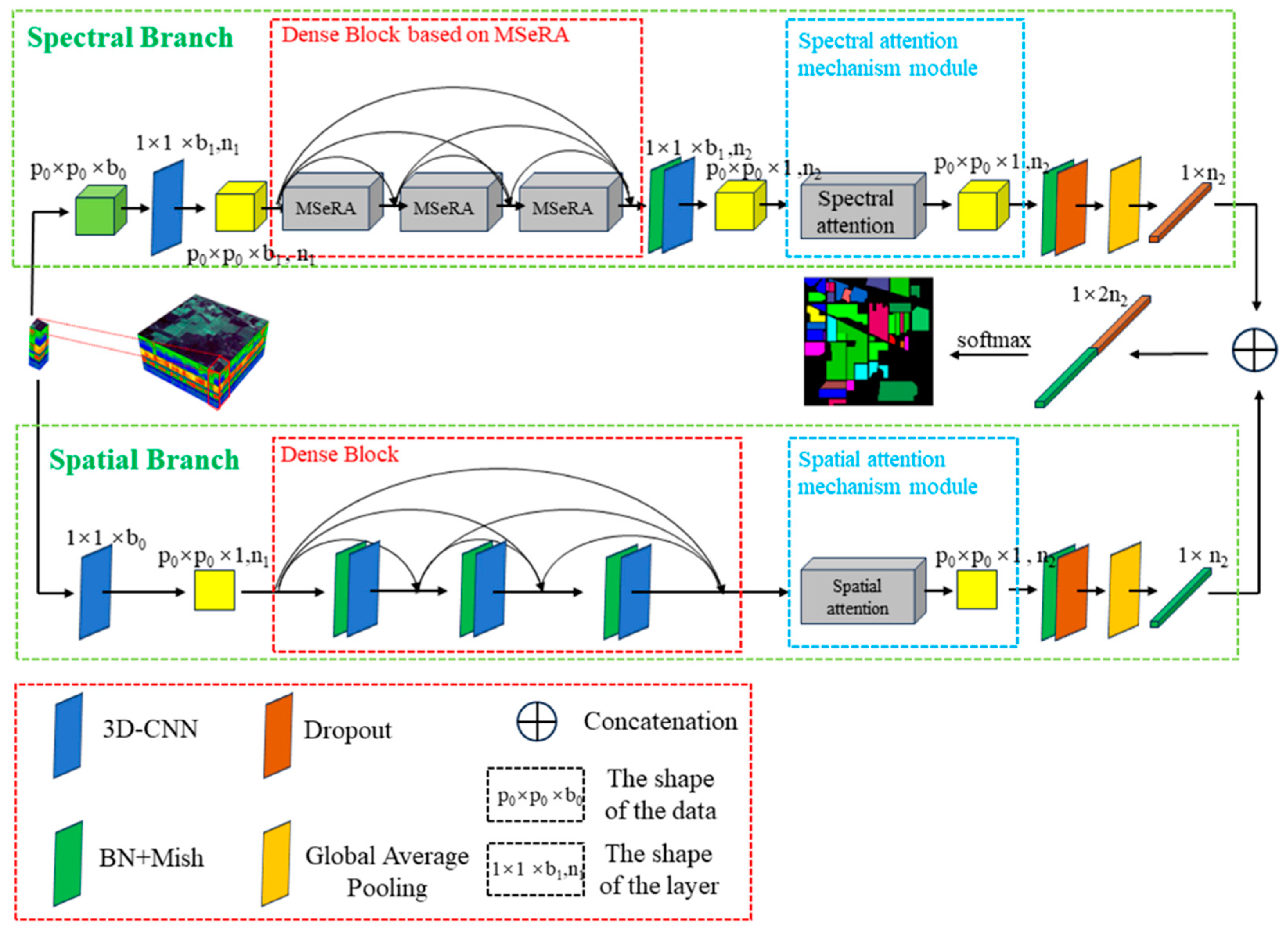
3.1. DBMSDA Network Framework

The overall structure of the DBMSDA network is shown in Figure 1. It consists of three main parts: the spectral branch, the spatial branch, and the classification head. The spectral branch is at the top of the model diagram, and the spatial branch is at the bottom. Finally, the two branches’ features are combined for classification. The spectral branch mainly consists of the MSeRA dense connection module and spectral attention module, while the spatial branch comprises the spatial dense connection module and spatial attention module. The overall framework adopts a “parallel form” double-branch structure, differing from the “series form” single-branch network framework used by FDSSC [45] (where spectral information is first extracted, followed by spatial information). A single-branch network may cause spectral and spatial features of HSI data to be in different domains, potentially leading to the destruction of spatial features extracted later [40]. Since HSI data are stored as a three-dimensional cube, traditional 1D-CNN can only capture spectral information, while 2D-CNN can only capture spatial information to some extent [37]. Neither can effectively extract both spectral and spatial information simultaneously. However, 3D-CNN can extract both types of information concurrently, providing clear advantages in processing three-dimensional structural data like HSI. Therefore, this article uses 3D-CNN as the fundamental convolutional structure of the DBMSDA network to extract HSI features. The network input size is $P\in R^{p_0\times p_0\times b_0}$. To prevent data explosion and gradient disappearance, BN + Mish [17] is used to standardize the results after each convolution in dense connections. To extract as many useful features as possible, a self-attention mechanism is added after dense connections to emphasize important features. Then, the dropout layer and global average pooling layer are used to convert the cubic feature maps from the two branches into one-dimensional vector features. Finally, the two one-dimensional vector features are combined, and the linear layer is used for classification.

3.2. Spectral Feature Extraction Module Based on MSeRA Structure

3.2.1. MSeRA Structure

Although deep learning algorithms have achieved remarkable results in HSI classification, most methods only consider features on a single scale. Many experiments have confirmed that multi-scale features play a crucial role in HSI classification [29,32,46].

Based on the concepts of multi-scale and attention, this article introduces a multi-scale residual self-attention (MSeRA) structure, as illustrated in Figure 2. The MSeRA structure is a branching structure containing three convolution kernels of different sizes. This article uses a 1 × 1 × 1 convolutional layer as the initial component of the MSeRA structure to increase the input size. Then, a multi-scale convolution group is used for feature extraction. A convolutional group with three convolution kernels of different sizes (1 × 1 × b, where b₁ = 3, b₂ = 5, b₃ = 7) is selected to construct feature representations at different scales. By utilizing multi-scale spectral dense blocks, the network can capture various levels of spectral features aligned with multiple receptive fields in each channel. This approach enables the network to gather more comprehensive spectral information, enhancing classification performance. The different output feature maps obtained at the three scales are then combined to obtain the fused feature. To address the issue of vanishing network gradients, this article uses skip connections to generate residual maps. This connection links the initial input features with the fused features to prevent gradient vanishing and information loss, enhancing the network’s expressive power. The spectral self-attention mechanism is then utilized to highlight valuable multi-scale spectral information and mitigate the impact of redundant data. The spectral self-attention mechanism here is consistent with the spectral attention block in Section 3.4.1 of the Spectral Attention Module. Finally, all feature maps are passed through a 1 × 1 × 1 convolutional layer to ensure consistent dimensions. The MSeRA structure can effectively extract spectral information from hyperspectral images, which contain rich features at various scales. It can also learn adequate and diagnostic spectral features from a small number of samples, enabling the network to achieve good results even with limited training samples.

3.2.2. Dense Block Based on MSeRA

Generally, according to the architectural principles of deep convolutional neural networks, increasing the number of convolutional layers and the stacking depth improves network performance. However, experiments show that having too many convolutional layers can result in gradient disappearance and gradient explosion. Dense connections [47] are an effective approach to address these issues.

Dense connections differ from residual connections [48]. Residual connections can be viewed as a mapping that allows input data to pass directly through the network [17], as illustrated in Figure 3a. Dense connections, proposed based on residual connections, directly link each layer to ensure a maximum information exchange between network layers, as illustrated in Figure 3b. The denser the connections, the more information flows through them. Specifically, a dense connection with N layers has N(N + 1)/2 connections, while a traditional convolutional network with the same number of layers has only N direct connections [17].

The residual block is the fundamental unit of a residual connection, and the output of the i-th residual block is represented as

$$x_i=N_i\left(x_{i-1}\right)+x_{i-1}$$

(1)

Dense blocks are the fundamental components of dense connections. Traditional residual connections combine features by summing or connecting adjacent (two) features, while dense connections combine features by connecting across multiple channel dimensions. The output of the i-th dense block is represented as

$$x_i=N_i\left[x_0,x_1,\dots ,x_{i-1}\right]$$

(2)

Among them, $N_i$ is the module containing the convolution layer, activation layer, and BN layer; $x_0,x_1,\dots ,x_{i-1}$ is the feature map generated by the above dense block.

The dense connection module, based on the MSeRA structure proposed in this article, facilitates information flow between layers by densely connecting the MSeRA modules. It helps obtain spectral information from the original HSI data to the fullest extent and prevents gradient disappearance and explosion.

3.3. Spatial Feature Extraction Module

Due to the high-dimensional features of HSI data, shallow neural networks struggle to extract deep spatial features from hyperspectral images. Dense connections are also utilized here to establish information flow between different layers, preventing the loss of spatial information.

The structure of the densely connected modules in the spatial branch is similar to that in the spectral branch. However, the dense block unit in the spatial branch does not utilize a multi-scale residual self-attention structure like MSeRA. Instead, it comprises a simple 3D-CNN, BN layer, and Mish activation function. This design avoids distorting the learned spectral features with excessive spatial information. HSI classification primarily relies on spectral information, with spatial information playing a supporting role. Excessive spatial information can increase the difficulty of extracting spectral information [19].

3.4. Attention Mechanism

The attention mechanism automatically learns and selectively focuses on important information in the input, enhancing the model’s performance and generalization ability. Although 3D-CNN can effectively extract spectral and spatial information in HSI, convolution has a common flaw: invariance. This flaw is evident in that all spatial pixels are assigned equal weights in the spatial domain, and all spectral bands are given equal weights in the spectral domain. However, HSI involves a large number of spatial pixels and spectral bands, and it is important to note that different spatial pixels and spectral bands do not make the same contribution. The attention mechanism effectively addresses this problem. Its main function is to emphasize important information areas and ignore unimportant ones. Currently, the attention mechanism is widely used in various fields. To address various issues, researchers have developed a variety of attention modules. In DANet [49], the spectral attention block and spatial attention block, based on the self-attention mechanism, enhance the weight of important spectral and spatial information. The self-attention mechanism was first proposed and used in NLP [50]. Its main function is to model remote dependencies. Subsequently, the CV field recognized the significant potential of the self-attention mechanism and began extensive research and applications [19,50,51]. These two modules will be introduced in detail below.

3.4.1. Spectral Attention Module

Research shows that spectral information is the basis of HSI processing and determines the final classification performance [43,52]. Different ground object categories can be represented by corresponding high-level features. High-level features in the spectral of HSI data are often represented by channels, and different channels of HSI data often exhibit certain correlations. We can utilize their correlations to highlight interdependence [49]. As shown in Figure 4a, the channel attention map $X\in R^{c\times c}$ is directly calculated from the original feature $A\in R^{c\times p\times p}$, where the number of input channels is represented by c, The size of the input patch is expressed as p × p. Specifically, we need to first perform matrix multiplication of A in the form of $R^{c\times n}$ with A^T, where n = p × p, and then use the SoftMax operation to obtain the channel attention mapping in the form of $X\in R^{c\times c}$:

$$x_{ji}=\frac{exp\left(A_i\times A_j\right)}{{\displaystyle {\sum }_{i=1}^{c}exp\left(A_i\times A_j\right)}}$$

(3)

where x_ji represents the influence of the i-th channel on the j-th channel. Then, perform matrix multiplication of X^T with A and reshape the result into $E\in R^{c\times p\times p}$:

$$E_j=\alpha {\displaystyle {\sum }_{i=1}^c\left(x_{ji}{A}_j\right)+A_j}$$

(4)

where α is initialized to 0 and can be learned to change values in the network. The final mapping E contains the weighted sum of all channel features and original features. This reflects the long-term semantic dependence between feature maps, enhancing the discriminability of features. Compared to the traditional channel attention mechanism (CAM), the spectral attention mechanism discussed in this article falls under self-attention mechanisms. This self-attention mechanism enables the extraction of dependency relationships among different spectra, facilitating the acquisition of global spectral context information. CAM only determines the significance of each channel by utilizing global maximum pooling and global average pooling across the spatial dimensions. Moreover, the strong correlation between hyperspectral image spectra cannot be captured by CAM.

3.4.2. Spatial Attention Module

Research shows that spatial features also play an important auxiliary role in HSI classification [43,52]. The spatial attention module can enhance the contextual relationship of local features. As shown in Figure 4b, two convolutional layers are used to perform a convolution operation on the input feature map $A\in R^{c\times p\times p}$ to obtain new feature maps B and C, where $\left\{B,C\right\}\in R^{c\times p\times p}$. Then reshape B and C into $R^{c\times n}$ and $R^{n\times c}$, where n = p × p represents the number of pixels. Then perform matrix multiplication on B and C, and use the SoftMax operation to calculate the spatial attention feature map $S\in R^{n\times n}$:

$$s_{ji}=\frac{exp\left(B_i\times C_j\right)}{{\displaystyle {\sum }_{i=1}^{n}exp\left(B_i\times C_j\right)}}$$

(5)

where s_ji represents the influence of the i-th pixel on the j-th pixel. The stronger the correlation, the closer the feature representations of two pixels.

At the same time, a convolution layer is used to perform a convolution operation on the initial input feature A to obtain a new feature map and reshape it into $R^{n\times c}$. Then matrix multiplication is performed on D and S^T, and the result is reshaped into $R^{c\times p\times p}$. Finally, we multiply it by the scale parameter β and perform a summation operation with the initial feature A to obtain the final output $E\in R^{c\times p\times p}$:

$$E_j=\beta {\displaystyle {\sum }_{i=1}^n\left(s_{ji}{D}_j\right)+A_j}$$

(6)

where β is initialized to 0 and learns to assign more weights in the network. The obtained result E is the weighted sum of all location features and original features, which can reflect the spatial global context information. Compared to the traditional spatial attention mechanism (SAM), the spatial attention mechanism discussed in this article is a self-attention mechanism. This self-attention mechanism captures the dependency relationships between various spatial locations, enabling the extraction of comprehensive global spatial context information. While SAM captures the significance of spatial regions using global max-pooling and global average pooling in the channel dimension, it overlooks the impact of global contextual information on classification.

4. Results

In this section, we evaluate the effectiveness of the proposed DBMSDA network model on multiple datasets. We compare the proposed method with several typical and state-of-the-art HSI classification algorithms while ensuring no information leakage.

4.1. Datasets Description

To validate the effectiveness of our proposed method and enable fair comparison with existing approaches, we conducted performance evaluations on a self-constructed lithology dataset and three widely recognized public datasets: KY, Houston_2018 (Hu), Indian Pines (IN), and Salinas Valley (SV). These datasets are outlined as follows:

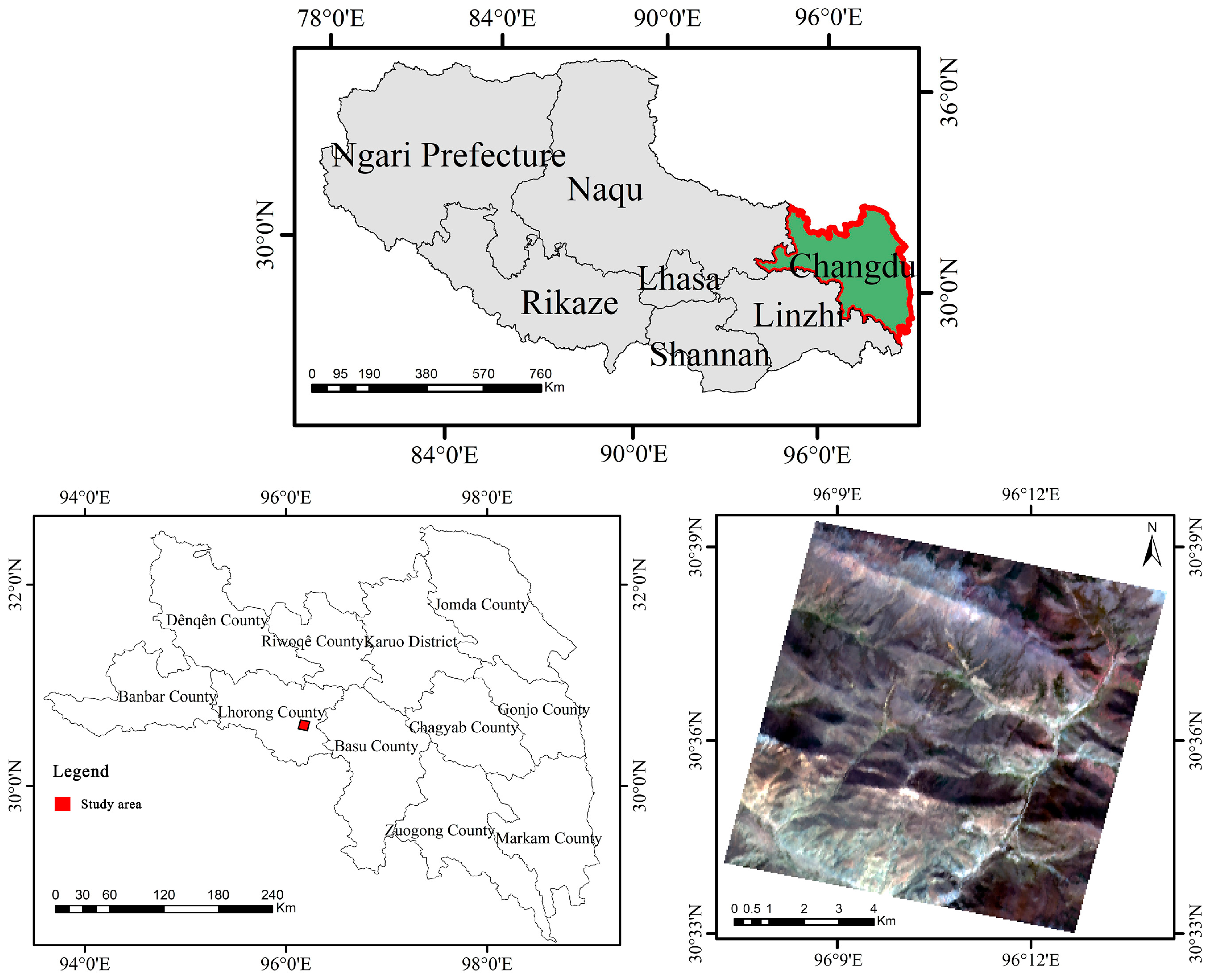
• KY dataset: This hyperspectral lithology dataset was created using ENVI 5.3 software, MATLAB R2021b software, manual interpretation, and field surveys with data from the Zhiyuan-1 remote sensing satellite. The data were collected in the eastern part of Luolong County, Changdu City, Tibet Autonomous Region, China (Figure 5). The image has a spatial resolution of 30 m. The original remote sensing image covers an area of 147 square kilometers, situated between latitudes 30°33′–30°40′N and longitudes 96°07′–96°14′E. The terrain is predominantly bare mountains. The image has spatial dimensions of 300 × 300 and consists of 166 bands. Excluding background pixels, the number of spatial pixels used for the experiment is 89,981. There are six types of real ground objects, mainly consisting of various surface lithologies such as sand and gravel, mudstone, sandstone, quartz sandstone, slate, schist, and phyllite. These represent different surface outcrop lithologies, with detailed information provided in Figure 6. There is a clear imbalance in the number of samples from different categories. The average training pixels account for 4.5% of the labeled pixels.
• Houston_2018 (Hu) dataset: This dataset was collected using an airborne hyperspectral sensor over the University of Houston campus and adjacent urban areas in 2018. The image has spatial dimensions of 601 × 2384 and consists of 50 bands. Excluding background pixels, there are 504,856 spatial pixels used for experiments. There are 20 types of ground objects, mainly buildings, vegetation, and urban ground objects. Detailed information is provided in Figure 6. There is a noticeable imbalance in the number of samples among different classes. The average training pixels account for 1% of labeled pixels.
• Indian Pines (IN) dataset: This dataset was collected using the AVIRIS sensor in the Indian Pines region of northwest India in 1992. The image has spatial dimensions of 145 × 145, consists of 220 bands, and covers a wavelength range of 200–400 nm. The spectral and spatial resolutions are 10 nm and 20 m, respectively. Excluding background pixels, there are 10,249 spatial pixels used for experiments. There are 16 types of ground objects, primarily crops and vegetation, with a small number of buildings and other objects. Detailed information is provided in Figure 6. Due to the unavailability of 20 bands, the experiment only utilizes the remaining 200 bands out of the total 220 for research. There is a noticeable imbalance in the number of samples among different classes. The average training pixels account for 11.59% of labeled pixels.
• Salinas Valley (SV) dataset: This dataset was collected using the AVIRIS sensor in Salinas Valley, California, USA in 1998. The image has spatial dimensions of 512 × 217, with a total of 224 bands. However, 20 water absorption bands were excluded, leaving 204 bands for hyperspectral image classification experiments. The spatial resolution is 1.7 m. Excluding background pixels, there are 54,129 spatial pixels used for experiments. There are 16 types of ground objects, mainly including vegetables, bare soil, and vineyards. Detailed information is provided in Figure 6. There is no imbalance in the number of samples among different classes. The average training pixels account for 4.3% of labeled pixels.

4.2. Datasets Partitioning Strategy

Many studies have shown that the traditional patch-based random partitioning method of hyperspectral datasets may lead to potential information leakage between the training set and the test set [41,43,44]. To prevent this problem and ensure a fairer evaluation of the network model’s classification performance, this article adopts the information leakage-free dataset partitioning method proposed by [11]. The specific steps are as follows:

• First, determine the α parameter and β parameter. The α parameter represents the proportion of training pixels to all pixels in the original hyperspectral image, while the β parameter indicates the number of labeled pixels in each training block. From the above two parameters, we can know that the number of training blocks in each category is $F_i=f_i\times \alpha ÷\beta$. Where i represents the category of each pixel, F_i represents the number of training blocks in the corresponding pixel category $F_i\ge 1$, and f_i represents the total number of pixels of each category in the original hyperspectral image.
• According to the training pixel ratio α, the original hyperspectral image can be divided into two parts. One part is the training image, and the other part is the verification–test image. There is no overlap between these two images.
• According to the number of labeled pixels β in each training block, the training image is divided into two parts. One part is defined as the training image, which is guaranteed to have labeled pixels, while the other part is defined as the leaked image. Similarly, the verification–test image is divided into a verification image and a test image.
• Divide the acquired training image, leaked image, verification image and test image into blocks of W × H × B size to generate training blocks, leaked blocks, verification blocks and test blocks.
• Finally, the sliding window strategy is used to divide the training patches, verification patches, and test patches from the blocks. These patches constitute the final training set, validation set, and test set.

4.3. Experimental Settings (Evaluation Indicators, Parameter Configuration, and Networkconfiguration)

In the experiment, multiple trials were conducted to investigate the impact of different learning rates on the outcome. The learning rates selected were 0.001, 0.005, 0.0001, 0.0005, and 0.00005. The optimal learning rate for multiple datasets was found to be 0.0005. The experimental epoch was set to 100, and the batch size was set to 64. The hardware used in the experiment included an Intel(R) Core(TM) i5-13400F CPU, NVIDIA GeForce RTX 3060 Ti GPU, and 32 GB of memory. The software environment included CUDA 12.2, PyTorch 2.0.1, and Python 3.10.11. In the experiment, the method described in this article was compared with classic and newer network models, including CDCNN, SSRN, SSTN, DBMA, DBDA, DRIN, SSFTT, SpectralFormer, FactoFormer, HyperBCS, 3DCT, DBMSDA (sub-1), and DBMSDA (sub-2).

To evaluate the robustness and effectiveness of the network model, this article uses overall accuracy (OA), average accuracy (AA), and the Kappa coefficient as performance indicators, averaging the results of 10 experiments. These three evaluation metrics collectively reflect the performance of the hyperspectral image classification model. Higher values in these metrics indicate better model performance. Let $M\in R^{n\times n}$ denote the confusion matrix of the classification result, where n denotes the number of categories, and the value of M at the (i, j) position denotes the number of samples of the i-th category that have been classified into the j-th category.

The overall accuracy (OA) is calculated as the ratio of the total number of correctly classified pixels (excluding the background class) to the total number of all accurately annotated pixels. This metric evaluates the model’s overall classification performance on hyperspectral images. The calculation formula is as follows:

$$OA=sum(diag(M)./sum(M))$$

(7)

The average accuracy (AA) is calculated as the average ratio of the total number of correctly categorized pixels for each category (excluding the background category) to the total number of pixels of each category with true annotations. This metric reflects the model’s accuracy in categorizing pixels for each category and, when combined with OA, provides a comprehensive evaluation of the model’s performance. The calculation formula is as follows:

$$AA=mean(diag(M)./sum(M,2))$$

(8)

In addition to OA and AA, the Kappa coefficient is also an important index for evaluating classification accuracy. It measures the consistency between the predicted results and the true value labels. The calculation formula is as follows:

$$Kappa=\frac{OA-(sum(M,1)sum(M,2))/sum{(M)}^2}{1-(sum(M,1)sum(M,2))/sum{(M)}^2}$$

(9)

In the above three formulas, $diag(M)\in R^{n\times 1}$ is the vector of diagonal elements of M, $sum(·)\in R^1$ is the sum of all the elements, $sum(\cdot ,1)\in R^{1\times n}$ is the vector of sums of elements in each column, $sum(\cdot ,2)\in R^{n\times 1}$ is the vector of sums of elements in each row, $mean(·)\in R^1$ is the average of all the elements, and $\cdot /$ denotes the division of the element dimension.

Among these factors, the size of blocks and patches used to divide the datasets significantly impacts the performance of the network model. o ensure a balance between the number of samples and spatial context information in the divided datasets, we set the block and patch sizes of the IN dataset to 6 × 6 and 4 × 4, the Hu dataset to 8 × 8 and 6 × 6, and the SV and KY datasets to 10 × 10 and 8 × 8, respectively.

The number of densely connected units in the MSeRA structure proposed in this article impacts classification accuracy. Therefore, we selected two, three, and four MSeRA modules to determine the optimal number. The experimental results are shown in Figure 7a. In the KY, Hu, IN, and SV datasets, the OA, AA, and Kappa values obtained with 2 and 4 MSeRA modules are lower than those obtained with three modules. From this, it is evident that using three MSeRA blocks more effectively extracts spectral features from hyperspectral images and achieves the best classification results.

The size of the multi-scale convolution group in the MSeRA module impacts classification accuracy. The size of various convolution kernels is related to the number and refinement of features that can be obtained. To further investigate the impact of multi-scale convolutional groups on classification performance, we selected combinations of convolution kernel sizes such as 1 × 1 × 3, 1 × 1 × 5, 1 × 1 × 7, and 1 × 1 × 5, 1 × 1 × 7, 1 × 1 × 9, and 1 × 1 × 7, 1 × 1 × 9, 1 × 1 × 11 to determine the optimal combination for convolution. The experimental results are shown in Figure 7b. Among these, the convolution kernel combinations of 1 × 1 × 3, 1 × 1 × 5, and 1 × 1 × 7 yielded better OA, AA, and Kappa scores in the KY, Hu, IN, and SV datasets than those of 1 × 1 × 5, 1 × 1 × 7, 1 × 1 × 9, and 1 × 1 × 7, 1 × 1 × 9, 1 × 1 × 11. Therefore, the best classification effect is achieved with the convolution kernel sizes of 1 × 1 × 3, 1 × 1 × 5, and 1 × 1 × 7 in the multi-scale convolution group.

4.4. Experimental Results and Analysis

This article compares the DBMSDA network with several classic and state-of-the-art networks. We used the same dataset partitioning strategy for all methods to prevent information leakage.

Table 1. Backbone structure of state-of-the-art HSI classification methods.

Network Name	Backbone Structure
CDCNN	2D-CNN + ResNet
SSRN	3D-CNN + ResNet
SSTN	3D-CNN + Transformer
DBMA	Parallel network + CBAM attention + DenseNet
DBDA	Parallel network + Self − attention + DenseNet
DRIN	Involution + ResNet
SSFTT	3D-CNN + Transformer + Gaussian − weighted feature tokenizer
SpectralFormer	CAF + GSE + Transformer, Based on ViT
FactoFormer	Factorized Transformers, Based on ViT
HyperBCS	3D-CNN + BSAM + CSM
3DCT	3D-CNN + ViT
DBMSDA	Parallel network + Self-attention + DenseNet + multi-scale feature extraction

lists the backbone structures used for training on the KY, Hu, IN, and SV datasets. Each network maintains the same training pixel ratio: KY at 4.5%, Hu at 1%, IN at 11.6%, and SV at 4.3%. Additionally, acknowledging the importance of joint spectral and spatial information in HSI classification, we designed two separate sub-networks within the DBMSDA network: one for the spectral branch and one for the spatial branch, to evaluate performance.

CDCNN [53]: This network model is primarily based on 2D-CNN and incorporates residual connections to address the issue of overly deep networks.

SSRN [37]: This network model is mainly based on 3D-CNN and incorporates residual connections, aimed at addressing the issue of overly deep networks. Additionally, 3D-CNN more effectively extracts hyperspectral “cube” structure data than 2D-CNN.

SSTN [15]: This network model is mainly based on 3D-CNN and introduces spatial attention and spectral correlation modules. The self-attention mechanism in spatial attention is used to acquire global context information and effectively extract hyperspectral data.

DBMA [40]: This network model features a double-branch structure that extracts both spectral and spatial information.

DBDA [17]: Based on DBMA, this network model also features a double-branch structure. It replaces the CBAM attention mechanism with a self-attention mechanism for improved acquisition of global context information.

DRIN [54]: This network model employs an involution structure to replace traditional convolution.

SSFTT [25]: This network model combines a convolutional network with a Transformer. It introduces a Gaussian distribution-weighted tokenization module to convert shallow spatial spectral features into tokenized semantic features, better representing the range from low to deep semantic features in HSI data.

SpectralFormer [19]: This network integrates group-wise spectral embedding (GSE) and cross-layer adaptive fusion (CAF) modules into the Transformer framework, aiming to enhance the capture of fine spectral differences and improve interlayer information transmission.

FactoFormer [55]: This network primarily uses factorized transformers to acquire spectral and spatial representations from hyperspectral data.

HyperBCS [56]: This network features a dual-scale addition module (BSAM) and a convolutional self-attention module (CSM). The BSAM module uses two branches to extract multi-scale features, while the CSM module integrates convolution and self-attention in a parallel structure to effectively extract both local and global features.

3DCT [57]: This network combines 3D-CNN and convolutional vision transformer (ViT) to enhance image recognition performance by leveraging CNN’s strengths in local feature extraction and transformers’ ability to process long-range dependencies.

DBMSDA (sub-1): This is the spectral branch of the DBMSDA network, a single-branch serial network with parameter settings consistent with the main DBMSDA network.

DBMSDA (sub-2): This is the spatial branch of the DBMSDA network, a single-branch serial network with parameter settings consistent with the main DBMSDA network.

4.4.1. Classification Results of KY Dataset

The average classification results from 10 independent repetitions using different methods on the KY dataset are shown in

Table 2. KY dataset: accuracy of each class, OA, AA (%), and Kappa index of classification results. Results are presented as mean.

Method
Class	CDCNN	SSRN	SSTN	DBMA	DBDA	DRIN	SSFTT	Spectral Former	Facto Former	Hyper BCS	3DCT	DBMSDA (sub-1)	DBMSDA (sub-2)	DBMSDA
C1	53.63	64.41	73.33	72.35	73.17	65.58	59.83	54.28	55.49	32.32	61.59	74.92	71.85	74.45
C2	69.84	68.99	67.70	74.13	73.77	67.11	61.93	68.92	68.63	54.90	63.31	75.56	69.56	76.35
C3	47.46	53.14	66.36	57.77	63.62	56.19	51.34	45.64	57.95	4.55	36.36	64.30	63.17	67.72
C4	82.39	89.05	89.78	89.70	93.19	92.46	91.65	84.12	88.13	83.74	87.48	92.14	91.59	93.73
C5	45.51	54.21	66.31	72.91	69.61	63.36	54.34	38.54	70.59	52.94	47.06	62.23	69.81	74.07
C6	91.67	50.00	75.00	66.67	100.00	100.00	50.00	50.00	100.00	100.00	100.00	100.00	75.00	100.00
OA	73.44	78.49	80.34	81.73	83.83	80.27	77.31	74.03	77.23	65.96	75.12	83.89	81.59	85.20
AA	65.08	63.30	73.08	72.25	78.89	74.12	61.51	56.91	73.46	54.74	65.97	78.18	73.49	84.09
Kappa	0.60	0.64	0.67	0.70	0.73	0.66	0.61	0.56	0.62	0.40	0.58	0.73	0.69	0.75

. The Ground Truth of the dataset and the classification diagrams obtained by different methods are shown in Figure 8.

From Table 2, the DBMSDA network achieves state-of-the-art classification performance, with the best results being OA 85.2%, AA 84.09%, and Kappa 0.75. As shown in Figure 8, the classification image obtained by the DBMSDA network is more accurate and smoother compared to other images.

From Figure 6, it is evident that the KY dataset exhibits a significant data imbalance, with the number of samples in class C6 being much smaller than in other classes. According to Table 2, when trained with only 4.5% of training pixels, the DBMSDA network not only ensures high classification accuracy for other classes but also achieves 100% accuracy in classifying a small number of class samples. This demonstrates that the DBMSDA network can effectively extract information from a small number of class samples under conditions of sample imbalance, thereby improving classification accuracy.

Specifically, the SSTN network, due to the introduction of the self-attention mechanism, achieved better classification results compared to the SSRN. This indicates that the global information obtained by the self-attention mechanism can indeed improve classification accuracy. Additionally, the DBMA and DBDA networks, being dual-branch network frameworks, outperformed the single-branch networks SSRN and SSTN. This suggests that dual-branch networks are generally superior to single-branch networks, possibly because single-branch networks may cause spectral and spatial information to mix and interfere with each other, potentially harming classification performance. Furthermore, SSFTT, SpectralFormer, FactoFormer, and 3DCT all adopted the Transformer framework, but their classification performance was poor, indicating that the Transformer framework may struggle with handling imbalanced sample data under dataset partitioning strategies without information leakage. Comparing the classification results of the two branches of the DBMSDA network, DBMSDA (sub-1) significantly outperformed DBMSDA (sub-2), indicating that spectral information is more important than spatial information in hyperspectral classification. Moreover, the DBMSDA network outperformed these two branches, indicating that the parallel dual-branch structure enhanced the interaction between spectral and spatial data, thereby improving classification performance. Overall, the DBMSDA network improved overall accuracy by 1.37%, average accuracy by 5.2%, and the Kappa coefficient by 0.023 compared to the DBDA network. Through the comparison of various networks, it is evident that deep learning methods have broad prospects in the research and application of hyperspectral geological lithology identification. Particularly, the DBMSDA network demonstrates superior classification performance under conditions of imbalanced sample data.

4.4.2. Classification Results of Hu Dataset

The average classification results from 10 independent repetitions using different methods on the Hu dataset are shown in

Table 3. Hu dataset: accuracy of each class, OA, AA (%), and Kappa index of classification results. Results are presented as mean.

Method
Class	CDCNN	SSRN	SSTN	DBMA	DBDA	DRIN	SSFTT	Spectral Former	Facto Former	Hyper BCS	3DCT	DBMSDA (sub-1)	DBMSDA (sub-2)	DBMSDA
C1	44.09	51.79	46.85	57.01	55.90	60.25	55.40	32.65	28.34	39.95	52.16	52.36	51.68	52.40
C2	63.89	63.26	61.90	67.31	68.25	61.34	72.90	68.11	66.03	62.58	66.91	68.60	60.98	71.10
C3	88.13	58.54	75.29	89.17	93.69	61.36	62.26	94.91	84.02	81.45	86.39	77.64	86.70	93.08
C4	50.01	46.06	45.67	58.62	58.01	67.41	63.25	48.00	49.38	37.23	64.32	52.00	50.56	61.22
C5	29.44	21.28	31.11	37.51	43.84	25.70	36.20	23.94	20.43	14.39	35.12	35.18	36.73	35.28
C6	40.58	35.75	40.32	41.29	46.63	48.20	30.93	33.75	41.57	27.17	39.38	43.63	42.41	47.63
C7	33.41	33.81	31.65	34.09	34.55	25.45	22.05	31.19	32.73	28.73	31.93	42.78	30.63	36.99
C8	59.69	41.26	53.18	66.25	67.40	63.39	59.96	58.61	62.33	50.03	57.56	57.71	55.40	71.02
C9	82.16	84.21	83.06	85.15	86.87	62.68	79.97	82.20	82.94	82.25	84.40	86.43	85.14	85.96
C10	25.23	21.61	24.85	23.74	24.92	30.14	27.28	23.87	22.32	22.94	25.47	28.45	26.05	29.97
C11	30.78	27.18	29.53	31.57	36.68	33.47	31.95	23.05	24.97	23.88	29.19	32.56	30.84	34.53
C12	3.49	0.93	4.04	2.08	1.79	1.95	1.57	3.67	2.54	1.28	1.30	2.88	2.49	2.11
C13	34.36	38.51	44.74	49.25	49.09	60.48	41.10	34.65	43.57	43.67	35.72	59.50	40.52	54.40
C14	36.76	28.57	52.04	48.72	54.95	4.35	39.72	27.99	33.38	30.76	36.19	51.35	50.70	51.25
C15	47.96	43.61	47.23	65.03	64.02	29.39	66.41	28.51	43.70	32.60	66.78	56.49	52.89	70.70
C16	30.29	27.85	36.11	47.79	51.71	34.26	28.75	25.20	26.33	21.06	37.85	48.20	37.70	51.08
C17	55.55	78.88	71.86	80.66	76.50	50.00	52.90	28.67	55.98	41.70	64.05	90.34	74.73	89.70
C18	48.75	41.04	58.92	64.40	66.02	36.00	24.86	38.98	30.05	23.36	30.57	64.17	54.79	73.65
C19	40.91	45.82	65.57	63.44	62.90	22.30	30.89	30.69	41.29	22.97	31.95	61.74	61.09	57.97
C20	42.58	43.28	51.06	54.09	56.82	50.92	37.30	49.13	29.49	43.70	41.67	57.51	56.53	56.40
OA	52.17	50.09	53.36	57.01	58.95	48.93	53.13	49.83	51.02	48.68	53.30	58.13	54.53	59.96
AA	44.40	41.66	47.74	53.35	55.03	42.45	43.28	39.38	41.07	36.58	45.95	53.47	49.43	56.32
Kappa	0.42	0.39	0.44	0.49	0.51	0.41	0.44	0.39	0.41	0.36	0.43	0.50	0.45	0.52

. The Ground Truth of the dataset and the classification diagrams obtained by different methods are shown in Figure 9.

From Table 3, it is evident that the Hu dataset includes a large amount of data across various land cover categories. However, due to the relatively small number of pixels selected for training, all networks exhibit relatively low classification performance. Despite these challenges, the DBMSDA network still achieved the highest classification performance, with the best results being OA 59.96%, AA 56.32%, and Kappa 0.52. From Figure 9, it is clear that the classification images obtained by the DBMSDA network are more accurate and smoother than those obtained by other networks.

From Figure 6, it is evident that the Hu dataset exhibits a significant data imbalance, with the sample sizes of categories C3, C7, C12, and C17 being much smaller than those of other categories. The classification results for the DBMSDA network are as follows: C3 class OA at 93.08%, C7 at 36.99%, C12 at 2.11%, and C17 at 89.7%. Specifically, the C12 class, identified as a pedestrian crossing, exhibits poor classification performance across all networks due to its narrow and short appearance compared to other objects. Overall, the DBMSDA network demonstrates relatively better classification performance for classes with small sample sizes. In Table 3, while the classification performance of the DBMSDA network for some small sample classes does not match DBMSDA (sub-1), it still ensures an overall improvement in accuracy. This suggests that the DBMSDA network’s structure, which integrates spectral and spatial information, is more versatile. Overall, compared to the DBDA network, the OA of the DBMSDA network improved by 1.01%, AA by 1.29%, and Kappa by 0.014.

4.4.3. Classification Results of IN Dataset

The average classification results from 10 independent repetitions using different methods on the IN dataset are displayed in

Table 4. IN dataset: accuracy of each class, OA, AA (%), and Kappa index of classification results. Results are presented as mean.

Method
Class	CDCNN	SSRN	SSTN	DBMA	DBDA	DRIN	SSFTT	Spectral Former	Facto Former	Hyper BCS	3DCT	DBMSDA (sub-1)	DBMSDA (sub-2)	DBMSDA
C1	33.33	45.14	40.14	33.47	81.67	39.45	18.06	15.19	23.96	0.00	11.67	77.92	52.08	88.33
C2	64.32	69.79	76.87	72.34	78.32	71.31	47.74	65.10	73.11	29.49	57.98	80.90	69.75	80.45
C3	63.10	64.31	74.50	71.28	75.74	70.02	53.00	60.84	66.89	27.05	43.74	77.83	67.78	79.05
C4	48.48	31.26	50.75	50.31	54.29	50.53	26.56	42.54	56.98	17.25	25.13	48.45	51.74	53.67
C5	66.78	70.94	72.95	70.42	73.25	68.56	68.34	55.72	63.55	65.98	64.56	75.53	72.69	73.60
C6	83.33	89.39	83.62	86.73	89.10	77.98	81.43	80.39	85.40	58.56	88.15	93.41	83.33	92.85
C7	25.00	100.00	100.00	100.00	100.00	83.33	58.33	38.89	37.50	0.00	20.00	100.00	100.00	100.00
C8	90.62	94.82	94.31	94.09	97.62	95.18	88.64	82.36	96.02	83.88	94.29	99.00	96.18	99.67
C9	66.67	70.83	54.17	58.33	83.33	75.00	62.50	33.44	56.25	30.00	20.00	58.33	66.67	79.17
C10	60.06	71.55	71.58	74.25	77.41	72.53	52.71	68.98	68.65	37.70	60.24	90.11	73.84	87.77
C11	76.87	78.69	79.27	83.93	89.59	67.50	67.72	67.28	74.26	55.07	74.19	86.27	84.88	89.17
C12	46.49	55.02	63.21	64.99	73.42	59.11	32.42	53.68	57.35	22.69	36.93	76.01	66.34	75.23
C13	88.79	85.85	89.15	84.72	90.08	87.90	81.35	76.60	86.01	55.39	84.23	90.08	90.08	90.08
C14	87.55	90.69	94.04	91.71	92.59	89.44	88.31	82.38	88.05	85.09	93.39	92.20	92.57	93.42
C15	70.30	71.07	61.87	63.98	75.50	63.75	46.63	51.13	65.02	17.92	44.07	74.91	68.02	74.98
C16	75.48	86.67	63.37	74.48	74.72	84.17	59.72	70.60	46.90	37.24	74.14	84.72	66.31	86.94
OA	71.01	75.03	77.45	77.77	82.76	72.39	62.32	75.01	73.40	47.60	66.39	84.26	77.73	84.92
AA	65.45	73.50	73.11	73.44	81.66	72.23	58.34	66.09	65.36	38.95	55.79	81.60	75.11	83.76
Kappa	0.67	0.72	0.74	0.75	0.80	0.69	0.57	0.72	0.70	0.40	0.61	0.82	0.75	0.83

. The average classification results from 10 independent repetitions using different methods on the IN dataset are displayed in Table 4. The Ground Truth and classification diagrams obtained by different methods are shown in Figure 10.

From Table 4, the DBMSDA network has achieved state-of-the-art classification performance, with the best results being OA 84.92%, AA 83.76%, and Kappa 0.83. From Figure 10, the classification images obtained by the DBMSDA network are noticeably more accurate and smoother than those from other networks.

Figure 6 reveals a significant data imbalance in the IN dataset, with notably fewer samples in classes C1, C7, C9, and C16 compared to other classes. According to Table 4, the DBMSDA network exhibits superior classification accuracy in the C1, C7, C9, and C16 categories compared to other networks. Specifically, the OA for class C1 is 88.33%, the highest recorded, while class C7 achieves 100% accuracy, also the highest among all classes. Class C9 reaches 79.17% accuracy, surpassed only by the DBDA network. However, the variability in classification results across classes is greater in the DBDA network than in the DBMSDA network, possibly affecting representativeness. Class C16 achieves an accuracy of 86.94%, only outperformed by the DA-IMRN network, whose overall classification accuracy remains lower than the DBMSDA network. These results demonstrate that the DBMSDA network effectively extracts information from limited class samples, even in the presence of unbalanced sample sizes. This enhances classification accuracy for smaller classes, thereby improving overall accuracy. The classification performance across networks is generally consistent with results observed in the KY dataset. Overall, the OA of the DBMSDA network has increased by 2.16%, AA by 2.1%, and Kappa by 0.026 compared to the DBDA network.

4.4.4. Classification Results of SV Dataset

The average classification results from 10 independent repetitions using different methods on the SV dataset are displayed in

Table 5. SV dataset: accuracy of each class, OA, AA (%), and Kappa index of classification results. Results are presented as mean.

Method
Class	CDCNN	SSRN	SSTN	DBMA	DBDA	DRIN	SSFTT	Spectral Former	Facto Former	Hyper BCS	3DCT	DBMSDA (sub-1)	DBMSDA (sub-2)	DBMSDA
C1	85.55	96.06	95.84	95.25	95.62	94.21	91.85	84.21	82.98	100.00	90.05	97.99	97.21	97.21
C2	80.21	88.34	89.75	88.71	90.42	85.63	84.16	79.46	57.54	72.00	83.54	95.42	89.94	93.17
C3	77.94	93.38	94.28	90.92	94.49	84.68	77.31	81.69	69.91	57.14	82.74	96.32	91.84	95.09
C4	91.67	95.46	92.93	97.48	92.43	86.37	90.66	90.28	79.62	65.71	89.39	91.42	92.93	93.44
C5	86.48	83.85	87.83	82.88	86.56	91.96	87.90	81.47	85.17	92.00	89.27	85.15	86.61	84.11
C6	97.66	97.00	97.89	97.45	96.77	98.00	93.80	95.83	88.63	81.33	93.60	95.07	95.10	95.53
C7	83.28	88.87	88.45	86.79	88.64	87.45	84.21	84.96	82.15	84.93	89.02	93.59	88.80	91.09
C8	84.73	85.50	86.99	86.60	91.93	89.23	85.91	84.05	82.19	90.45	85.35	95.46	88.28	94.03
C9	90.45	86.18	98.96	97.70	98.82	94.20	94.51	89.29	88.66	81.51	92.97	99.58	97.90	99.08
C10	73.57	80.60	82.55	81.77	83.46	81.25	79.17	75.26	77.67	53.73	79.96	82.81	80.99	83.07
C11	71.62	74.74	75.45	72.34	78.91	79.68	78.68	65.31	71.11	41.67	73.80	85.21	79.62	81.73
C12	82.90	83.41	81.49	83.80	86.84	79.71	87.50	79.74	70.18	81.58	84.23	89.51	82.94	89.49
C13	82.66	81.23	82.04	81.66	83.19	82.40	85.71	79.03	84.84	52.38	82.37	82.45	83.90	82.42
C14	80.00	83.21	84.30	84.96	82.49	81.09	71.05	80.40	72.16	68.18	81.64	84.30	84.36	82.16
C15	58.65	80.69	76.60	72.18	82.71	52.28	66.93	61.04	66.07	9.32	55.03	85.37	69.91	83.86
C16	80.00	88.33	89.29	86.90	87.62	87.62	88.57	78.25	84.89	84.85	79.57	94.76	85.71	90.00
OA	81.55	87.76	88.30	86.98	90.10	84.37	84.39	81.04	78.28	70.73	82.85	92.30	87.34	91.22
AA	81.71	87.30	87.79	86.71	88.80	84.74	84.24	80.64	77.73	69.79	83.28	90.90	87.25	89.76
Kappa	0.80	0.87	0.87	0.86	0.89	0.83	0.83	0.79	0.76	0.68	0.81	0.92	0.86	0.90

. The Ground Truth and classification diagrams for this dataset, obtained by various methods, are presented in Figure 11.

From Table 5, it can be seen that the DBMSDA (sub-1) network framework achieved state-of-the-art performance, with the best results being an overall accuracy (OA) of 92.3%, an average accuracy (AA) of 90.9%, and a Kappa coefficient of 0.92. We speculate that this is due to the lack of sample imbalance in the SV dataset, where each terrain type has a sufficient and similar number of labeled pixels, leading to the DBMSDA’s classification results potentially not matching those of DBMSDA (sub-1). In this case, the introduction of spatial information may contaminate spectral information, resulting in a decline in classification performance. Similarly, for this reason, the dual-branch DBMA network’s classification performance falls short of the single-branch SSRN and SSTN networks in this dataset. However, typically, samples in hyperspectral images exhibit imbalanced distributions (as seen in the KY, Hu, and IN datasets), where the DBMSDA network usually performs better. Therefore, the DBMSDA network demonstrates broader generalization capabilities compared to DBMSDA (sub-1), and overall, DBMSDA still surpasses DBMSDA (sub-1). In general, the DBMSDA network has shown improvements over the DBDA network, with an increase in OA by 1.12%, AA by 0.96%, and Kappa by 0.012.

5. Discussion

The comparisons in Section 3 demonstrate that the proposed MSeRA structural feature learning, guided by the self-attention mechanism, yielded the best HSI classification results. This superiority was evident not only in the KY dataset but also in the public Hu, IN, and SV datasets. This article explores various factors influencing network model performance. It covers the effects of different block-patch sizes, performance variations based on training pixel counts, performance with minimal sample sizes, the impact of missing network modules on performance, a discussion on the time costs associated with various networks, and the effect of having or not having a dataset segmentation strategy.

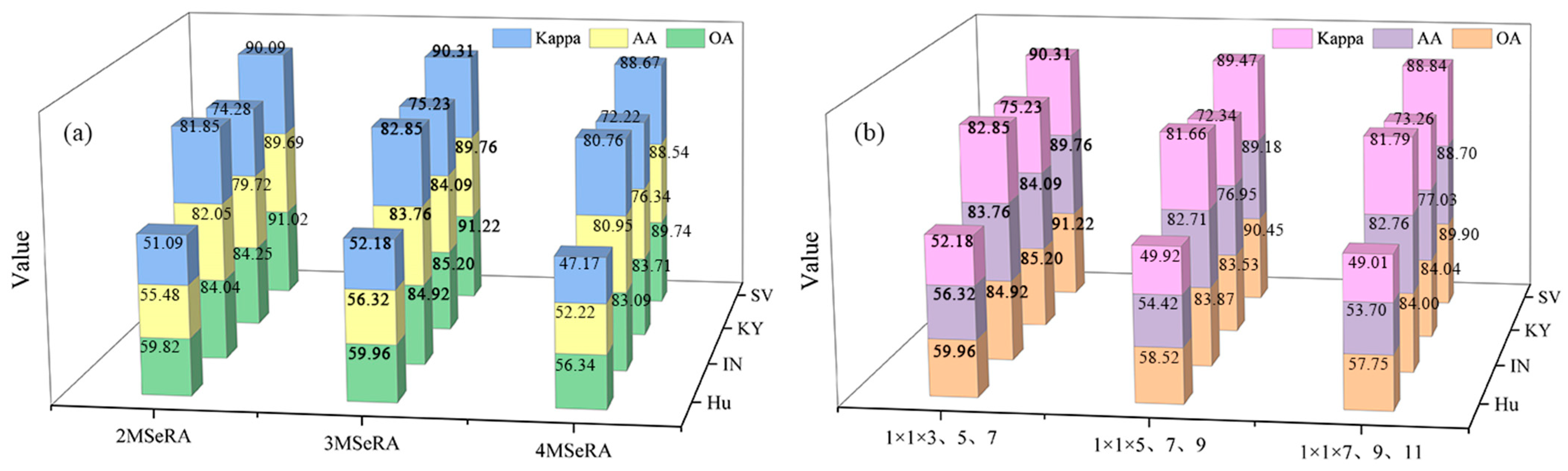
5.1. Effect of Block-Patch Size

The block-patch size is crucial in the dataset division method and significantly impacts the final classification result. Consequently, this article categorizes block-patch size combinations into several groups based on their significant impact. For the KY, Hu, and SV datasets with large spatial ranges, the block-patch sizes are divided into three types: 8-6, 10-8, and 12-10. For the IN dataset, which has a smaller spatial range, the block-patch sizes are divided into three types: 4-2, 6-4, and 8-6. The classification results, including OA and AA for these datasets, are shown in Figure 12.

Smaller block-patch sizes allocate more training samples to a single block but provide less overall spatial information, and vice versa. Therefore, optimal network performance depends on balancing the number of training samples with the amount of spatial information. For the KY, IN, and SV datasets, OA and AA values initially increase and then decrease, indicating an optimal block-patch size of 10-8 for KY. The optimal block-patch sizes are 6-4 for IN and 10-8 for SV. In the Hu dataset, with both OA and AA values decreasing, the optimal block-patch size is determined to be 8-6.

5.2. Impact of the Number of Labeled Training Pixels

The network’s performance is significantly influenced by the quantity of labeled training pixels; generally, as the number of labeled training pixels increases, so does the accuracy of network training. For the KY, Hu, IN, and SV datasets, we selected various labeled training pixel counts for comparative analysis. The selected training pixel ratios are as follows: 1%, 4.5%, 5%, and 10% for the KY dataset; 1%, 5%, 10%, and 15% for the Hu dataset; 1%, 5%, 10%, 11.6%, and 15% for the IN dataset; and 1%, 4.3%, 5%, and 10% for the SV dataset. Figure 13 displays the classification results for the four datasets using different methods at various training pixel ratios.

From Figure 13, with a low training pixel ratio of 1%, DBMSDA achieves the best classification results in the KY and Hu datasets. In the IN dataset, DBMSDA also achieves good results, but its performance in the SV dataset is less satisfactory. This underperformance in the SV dataset may be due to its relatively balanced sample distribution, which typically favors most convolutional neural networks. Therefore, the advantages of the DBMSDA network are not as apparent in this context. Additionally, networks like SpectralFormer, FactoFormer, and SSFTT, which use the Transformer framework, do not perform as well as double-branch networks such as DBMA and DBDA. This suggests that Transformer framework networks may underperform with small and unbalanced sample sizes, while double-branch networks tend to show better classification performance. Overall, the DBMSDA network proposed in this article shows the best classification performance across all four datasets. The DBMSDA network outperforms other methods in classification under conditions of small training sample sizes and sample imbalance, indicating superior generalization capabilities.

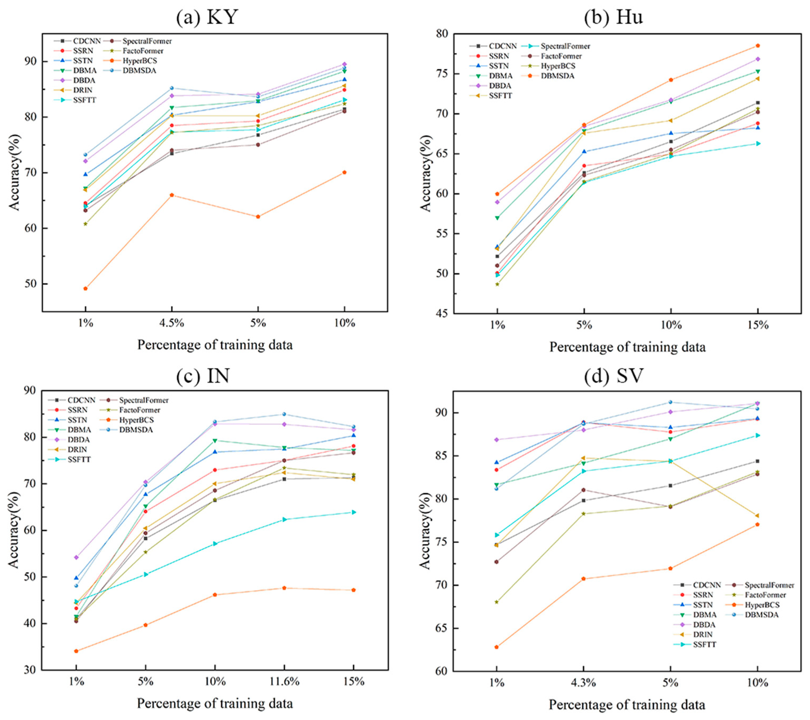
5.3. Classification Results of Networks in Minimal Sample Data

To demonstrate the classification performance of the DBMSDA network in extreme scenarios, such as with very limited sample data, we randomly selected approximately 10 pixels for each category from the KY, IN, and SV datasets as training pixels. Additionally, about 20 pixels for each category were selected from the Hu dataset as training pixels. We assessed the classification performance of the DBMSDA network and other networks using small sample data from these four datasets. The OA results for these datasets with small sample sizes are displayed in Figure 14.

From Figure 14, the DBMSDA network achieved the best classification results across all four datasets compared to other networks. Specifically, the OA results were 35.69% for the KY dataset, 26.06% for the Hu dataset, 50.17% for the IN dataset, and 74.13% for the SV dataset. Notably, the classification results for the SV and IN datasets were significantly better than those for the KY and Hu datasets. This could be because the KY dataset consists of lithology samples, which are highly similar, making accurate classification challenging with limited training samples. The Hu dataset, which contains numerous categories, shows subpar classification performance in scenarios with limited samples, likely exacerbated by the need to prevent information leakage. Even with limited training samples, the DBMSDA network’s classification results surpass those of other networks. This demonstrates the DBMSDA network’s ability to perform excellently under minimal sample conditions and to handle datasets with challenging class distinctions effectively.

5.4. Impact of Different Network Branches and Module Combinations

Furthermore, we analyze the effects of various suggested branch and module combinations.

Table 6. Ablation analysis of different branches/modules (OA %).

Branch	Spectral branch	✓		✓
	Spatial branch		✓	✓
Module	MSeRA				✓	✓	✓	✓
	MSaRA							✓
	Spectral attention				✓		✓	✓
	Spatial attention					✓	✓	✓
Data	KY	83.9	81.6	85.2	83.7	83.7	85.2	82.6
	Hu	58.1	54.5	60.0	59.7	58.6	60.0	59.1
	IN	84.3	77.7	84.9	84.1	84.1	84.9	83.1
	SV	92.3	87.3	91.2	90.7	90.6	91.2	89.5

displays the OA classification results for various branch and module combinations. The classification results show that the spectral branch alone outperforms the spatial branch alone. This suggests that spectral features are more significant than spatial features in the DBMSDA network. Integrating both spectral and spatial branches yields better classification results than using spectral branches alone, demonstrating that this combination is most effective for classifying hyperspectral data. In the SV dataset, the combined spectral and spatial branches slightly underperform compared to the spectral branch alone. This could be due to the lack of sample imbalance in the SV dataset, where incorporating spatial information may “contaminate” spectral information. The joint spectral and spatial branches perform better, indicating superior generalization capabilities. In the Hu dataset, the absence of branches and modules has minimal impact on classification accuracy. This may be attributed to the large number of categories and the small number of training samples, which contribute to overall low classification accuracy. Table 6 indicates that combining the MSeRA structure with spectral and spatial attention mechanisms yields the best classification performance. However, classification performance significantly decreases with the integration of the MSeRA and MSaRA modules, along with both spectral and spatial attention mechanisms. Excessive spatial information should be avoided as it complicates the extraction of spectral information and diminishes classification accuracy. It is important to note in particular that Columns 3 and 6 differ only in presentation; their underlying network frameworks are identical. So, the classification results obtained are the same. Column 3 denotes the impact of missing branches, and column 6 denotes the impact of missing modules.

5.5. Time Cost Comparison

The comparison of training and testing times for various network models, including our method, is presented in

Table 7. Training time in minutes (min) and test time in second(s) between the contrast methods and the proposed method on four datasets.

Methods	KY		Hu		IN		SV
	Train. (m)	Test (s)	Train. (m)	Test (s)	Train. (m)	Test (s)	Train. (m)	Test (s)
CDCNN	0.36	0.07	0.26	0.51	0.25	0.02	0.26	0.05
SSRN	2.70	0.20	0.49	0.94	3.40	0.05	2.10	0.20
SSTN	0.62	0.08	0.50	1.10	0.44	0.04	0.43	0.08
DBMA	4.05	0.38	0.73	1.39	1.24	0.08	3.13	0.37
DBDA	4.06	0.32	0.76	1.32	1.19	0.07	3.14	0.33
DRIN	0.51	0.09	0.38	1.10	0.32	0.03	0.36	0.08
SSFTT	0.48	0.06	0.31	0.73	0.26	0.02	0.35	0.05
SpectralFormer	1.68	0.15	0.62	1.27	1.53	0.08	1.33	0.15
FactoFormer	2.16	0.16	0.88	1.57	1.78	0.08	1.65	0.16
HyperBCS	655.20	74.00	19.20	66.00	24.58	2.00	656.52	105.00
3DCT	0.66	0.07	0.37	0.64	0.31	0.22	0.47	0.08
DBMSDA (sub-1)	172.82	5.60	4.17	9.08	11.66	0.50	170.68	7.42
DBMSDA (sub-2)	0.26	0.06	0.20	0.53	0.17	0.02	0.19	0.05
DBMSDA	172.89	5.62	4.23	9.22	11.64	0.51	174.07	7.59

. Although the DBMSDA method requires longer training and testing times compared to other methods, except for HyperBCS, it is designed to fully extract complex, high-dimensional spectral information from hyperspectral data. The spectral branch (sub-1) incurs significantly longer durations than the spatial branch (sub-2). Although the DBMSDA method incurs significant time costs, its performance with small sample sizes and unbalanced datasets is robust, which we consider acceptable.

5.6. The Effect of Having or Not Having a Dataset Segmentation Strategy

To verify the impact of a dataset partitioning strategy on network classification results, this study utilizes the DBMSDA network with the same number of training samples. One approach employs a dataset partitioning strategy, while the other does not. The classification results for the KY dataset are presented in

Table 8. The effect of having or not having a dataset partitioning strategy on the classification results and the corresponding classification results figure.

Class	Dataset Segmentation Strategy	No Dataset Segmentation Strategy
C1	77.44	98.70
C2	70.59	98.11
C3	68.18	93.62
C4	94.39	99.18
C5	94.12	100.00
C6	100.00	100.00
OA	84.66	98.61
AA	84.12	98.27
Kappa	0.743	0.978
GT	Dataset segmentation strategy	No dataset segmentation strategy

. Table 8 shows that the OA, AA, and Kappa values obtained using the dataset partitioning strategy are significantly lower than those obtained without it, by more than 10 percentage points for both OA and AA. However, the classification graphs show that the differences in results between using the dataset partitioning strategy and not using it are not significant. Notably, the result graphs without the dataset partitioning strategy show performances far from the desired classification accuracy of approximately 98%. Consequently, classification results without the dataset partitioning strategy are relatively high, leading to false positives. This discrepancy may stem from potential overlap between the training and test sets during classification. This overlap leads to information leakage. Therefore, adopting the dataset partitioning strategy ensures the credibility, fairness, and accuracy of the classification results.

6. Conclusions

Our research on previous articles has shown that the commonly used patch-wise dataset partitioning method in neural networks can lead to information leakage between the training and test sets. Therefore, we have implemented a novel dataset partitioning approach that prevents information leakage between the training and test sets. To fully extract spectral and spatial information from HSI data, we proposed the double-branch multi-scale dual-attention (DBMSDA) network, which prevents information leakage between the training and test sets. The network consists of two branches: the spectral and the spatial. The spatial branch uses convolutional dense connection modules and a spatial self-attention mechanism to extract spatial information. In the spectral branch, a multi-scale spectral residual self-attention (MSeRA) structure serves as a dense connection module, combined with a spectral self-attention mechanism to enhance dense connectivity. This integration enables a more comprehensive extraction of spectral information. We created a hyperspectral geological lithology dataset to explore the potential of deep learning methods in identifying hyperspectral geological lithologies. Experimental results show that the DBMSDA network not only outperforms other networks in hyperspectral geological lithology classification but also excels in public hyperspectral datasets. This demonstrates the promising research and application prospects of deep learning in hyperspectral geological lithology identification and highlights the superior classification performance and stronger generalization ability of the DBMSDA network compared to other networks.

Although the DBMSDA network shows good classification performance on datasets with small and unbalanced samples, it suffers from long training times and low efficiency. Therefore, future work will focus on enhancing hyperspectral image classification performance and reducing network model operation time. Additionally, future research will likely focus on integrating Transformer technology with double branch network frameworks.

References

1. Tong, Q.; Zhang, B.; Zhang, L. Current progress of hyperspectral remote sensing in China. J. Remote Sens. 2016, 20, 689–707. [Google Scholar]
2. Meyer, J.; Kokaly, R.; Holley, E. Hyperspectral remote sensing of white mica: A review of imaging and point-based spectrometer studies for mineral resources, with spectrometer design considerations. Remote Sens. Environ. 2022, 275, 113000. [Google Scholar] [CrossRef]
3. Nalepa, J.; Antoniak, M.; Myller, M.; Lorenzo, P.; Marcinkiewicz, M. Towards resource-frugal deep convolutional neural networks for hyperspectral image segmentation. Microprocess. Microsyst. 2020, 73, 102994. [Google Scholar] [CrossRef]
4. Kuras, A.; Brell, M.; Liland, K.; Burud, I. Multitemporal Feature-Level Fusion on Hyperspectral and LiDAR Data in the Urban Environment. Remote Sens. 2023, 15, 632. [Google Scholar] [CrossRef]
5. Yang, B.; Wang, S.; Li, S.; Zhou, B.; Zhao, F.; Ali, F.; He, H. Research and application of UAV-based hyperspectral remote sensing for smart city construction. Cogn. Robot. 2022, 2, 255–266. [Google Scholar] [CrossRef]
6. Arroyo-Mora, J.; Kalacska, M.; Inamdar, D.; Soffer, R.; Lucanus, O.; Gorman, J.; Naprstek, T.; Schaaf, E.; Ifimov, G.; Elmer, K.; et al. Implementation of a UAV–Hyperspectral Pushbroom Imager for Ecological Monitoring. Drones 2019, 3, 12. [Google Scholar] [CrossRef]
7. Liu, H.; Wu, K.; Xu, H.; Xu, Y. Lithology Classification Using TASI Thermal Infrared Hyperspectral Data with Convolutional Neural Networks. Remote Sens. 2021, 13, 3117. [Google Scholar] [CrossRef]
8. Ye, B.; Tian, S.; Cheng, Q.; Ge, Y. Application of Lithological Mapping Based on Advanced Hyperspectral Imager (AHSI) Imagery Onboard Gaofen-5 (GF-5) Satellite. Remote Sens. 2020, 12, 3990. [Google Scholar] [CrossRef]
9. Lin, N.; Fu, J.; Jiang, R.; Li, G.; Yang, Q. Lithological Classification by Hyperspectral Images Based on a Two-Layer XGBoost Model, Combined with a Greedy Algorithm. Remote Sens. 2023, 15, 3764. [Google Scholar] [CrossRef]
10. Zou, L.; Zhu, X.; Wu, C.; Liu, Y.; Qu, L. Spectral–Spatial Exploration for Hyperspectral Image Classification via the Fusion of Fully Convolutional Networks. IEEE J. Sel. Top. Appl. Earth Obs. Remote Sens. 2020, 13, 659–674. [Google Scholar] [CrossRef]
11. Qu, L.; Zhu, X.; Zheng, J.; Zou, L. Triple-Attention-Based Parallel Network for Hyperspectral Image Classification. Remote Sens. 2021, 13, 324. [Google Scholar] [CrossRef]
12. Ibañez, D.; Fernandez-Beltran, R.; Pla, F.; Yokoya, N. Masked Auto-Encoding Spectral–Spatial Transformer for Hyperspectral Image Classification. IEEE Trans. Geosci. Remote Sens. 2022, 60, 5542614. [Google Scholar] [CrossRef]
13. Li, N.; Wang, Z. Spatial Attention Guided Residual Attention Network for Hyperspectral Image Classification. IEEE Access 2022, 10, 9830–9847. [Google Scholar] [CrossRef]
14. Tan, Y.; Lu, L.; Bruzzone, L.; Guan, R.; Chang, Z.; Yang, C. Hyperspectral Band Selection for Lithologic Discrimination and Geological Mapping. IEEE J. Sel. Top. Appl. Earth Obs. Remote Sens. 2020, 13, 471–486. [Google Scholar] [CrossRef]
15. Zhong, Z.; Li, Y.; Ma, L.; Li, J.; Zheng, W. Spectral–Spatial Transformer Network for Hyperspectral Image Classification: A Factorized Architecture Search Framework. IEEE Trans. Geosci. Remote Sens. 2022, 60, 1–15. [Google Scholar] [CrossRef]
16. Mei, X.; Pan, E.; Ma, Y.; Dai, X.; Huang, J.; Fan, F.; Du, Q.; Zheng, H.; Ma, J. Spectral-Spatial Attention Networks for Hyperspectral Image Classification. Remote Sens. 2019, 11, 963. [Google Scholar] [CrossRef]
17. Li, R.; Zheng, S.; Duan, C.; Yang, Y.; Wang, X. Classification of Hyperspectral Image Based on Double-Branch Dual-Attention Mechanism Network. Remote Sens. 2020, 12, 582. [Google Scholar] [CrossRef]
18. Liu, Q.; Xiao, L.; Yang, J.; Chan, J. Content-Guided Convolutional Neural Network for Hyperspectral Image Classification. IEEE Trans. Geosci. Remote Sens. 2020, 58, 6124–6137. [Google Scholar] [CrossRef]
19. Hong, D.; Han, Z.; Yao, J.; Gao, L.; Zhang, B.; Plaza, A.; Chanussot, J. SpectralFormer: Rethinking Hyperspectral Image Classification with Transformers. IEEE Trans. Geosci. Remote Sens. 2022, 60, 5518615. [Google Scholar] [CrossRef]
20. Melgani, F.; Bruzzone, L. Classification of hyperspectral remote sensing images with support vector machines. IEEE Trans. Geosci. Remote Sens. 2004, 42, 1778–1790. [Google Scholar] [CrossRef]
21. Li, J.; Bioucas-Dias, J.; Plaza, A. Semisupervised hyperspectral image segmentation using multinomial logistic regression with active learning. IEEE Trans. Geosci. Remote Sens. 2010, 48, 4085–4098. [Google Scholar] [CrossRef]
22. Du, B.; Zhang, L. Target detection based on a dynamic subspace. Pattern Recog. 2014, 47, 344–358. [Google Scholar] [CrossRef]
23. He, L.; Li, J.; Liu, C.; Li, S. Recent Advances on Spectral–Spatial Hyperspectral Image Classification: An Overview and New Guidelines. IEEE Trans. Geosci. Remote Sens. 2018, 56, 1579–1597. [Google Scholar] [CrossRef]
24. Song, T.; Wang, Y.; Gao, C.; Chen, H.; Li, J. MSLAN: A Two-Branch Multidirectional Spectral–Spatial LSTM Attention Network for Hyperspectral Image Classification. IEEE Trans. Geosci. Remote Sens. 2022, 60, 5528814. [Google Scholar] [CrossRef]
25. Sun, L.; Zhao, G.; Zheng, Y.; Wu, Z. Spectral–Spatial Feature Tokenization Transformer for Hyperspectral Image Classification. IEEE Trans. Geosci. Remote Sens. 2022, 60, 5522214. [Google Scholar] [CrossRef]
26. Zou, J.; He, W.; Zhang, H. LESSFormer: Local-Enhanced Spectral-Spatial Transformer for Hyperspectral Image Classification. IEEE Trans. Geosci. Remote Sens. 2022, 60, 5535416. [Google Scholar] [CrossRef]
27. Yu, H.; Xu, Z.; Zheng, K.; Hong, D.; Yang, H.; Song, M. MSTNet: A Multilevel Spectral–Spatial Transformer Network for Hyperspectral Image Classification. IEEE Trans. Geosci. Remote Sens. 2022, 60, 5532513. [Google Scholar] [CrossRef]
28. Peng, Y.; Ren, J.; Wang, J.; Shi, M. Spectral-Swin Transformer with Spatial Feature Extraction Enhancement for Hyperspectral Image Classification. Remote Sens 2023, 15, 2696. [Google Scholar] [CrossRef]
29. Zou, L.; Zhang, Z.; Du, H.; Lei, M.; Xue, Y.; Wang, Z. DA-IMRN: Dual-Attention-Guided Interactive Multi-Scale Residual Network for Hyperspectral Image Classification. Remote Sens. 2022, 14, 530. [Google Scholar] [CrossRef]
30. Tao, H. Smoke Recognition in Satellite Imagery via an Attention Pyramid Network with Bidirectional Multilevel Multigranularity Feature Aggregation and Gated Fusion. IEEE Internet Things J. 2024, 11, 14047–14057. [Google Scholar] [CrossRef]
31. Tao, H.; Duan, Q.; Lu, M.; Hu, Z. Learning discriminative feature representation with pixel-level supervision for forest smoke recognition. Pattern Recognit. 2023, 143, 109761. [Google Scholar] [CrossRef]
32. Song, W.; Li, S.; Fang, L.; Lu, T. Hyperspectral Image Classification with Deep Feature Fusion Network. IEEE Trans. Geosci. Remote Sens. 2018, 56, 3173–3184. [Google Scholar] [CrossRef]
33. Ren, S.; Zhou, D.; He, S.; Feng, J.; Wang, X. Shunted self-attention via multi-scale token aggregation. In Proceedings of the IEEE/CVF Computer Vision and Pattern Recognition Conference (CVPR), New Orleans, LA, USA, 18–24 June 2022; pp. 10843–10852. [Google Scholar]
34. Qiao, X.; Roy, S.; Huang, W. Multiscale neighborhood attention transformer with optimized spatial pattern for hyperspectral image classification. IEEE Trans. Geosci. Remote Sens. 2023, 61, 5523815. [Google Scholar] [CrossRef]
35. Shi, C.; Yue, S.; Wang, L. A Dual-Branch Multiscale Transformer Network for Hyperspectral Image Classification. IEEE Trans. Geosci. Remote Sens. 2024, 62, 5504520. [Google Scholar] [CrossRef]
36. Feng, H.; Wang, Y.; Li, Z.; Zhang, N.; Zhang, Y.; Gao, Y. Information Leakage in Deep Learning-Based Hyperspectral Image Classification: A Survey. Remote Sens. 2023, 15, 3793. [Google Scholar] [CrossRef]
37. Zhong, Z.; Li, J.; Luo, Z.; Chapman, M. Spectral–Spatial Residual Network for Hyperspectral Image Classification: A 3-D Deep Learning Framework. IEEE Trans. Geosci. Remote Sens. 2018, 56, 847–858. [Google Scholar] [CrossRef]
38. Hang, R.; Li, Z.; Liu, Q.; Ghamisi, P.; Bhattacharyya, S. Hyperspectral Image Classification with Attention-Aided CNNs. IEEE Trans. Geosci. Remote Sens. 2021, 59, 2281–2293. [Google Scholar] [CrossRef]
39. Zhang, Z.; Liu, D.; Gao, D.; Shi, G. S³Net: Spectral–Spatial–Semantic Network for Hyperspectral Image Classification with the Multiway Attention Mechanism. IEEE Trans. Geosci. Remote Sens. 2022, 60, 5505317. [Google Scholar]
40. Ma, W.; Yang, Q.; Wu, Y.; Zhao, W.; Zhang, X. Double-Branch Multi-Attention Mechanism Network for Hyperspectral Image Classification. Remote Sens. 2019, 11, 1307. [Google Scholar] [CrossRef]
41. Liang, J.; Zhou, J.; Qian, Y.; Wen, L.; Bai, X.; Gao, Y. On the Sampling Strategy for Evaluation of Spectral-Spatial Methods in Hyperspectral Image Classification. IEEE Trans. Geosci. Remote Sens. 2017, 55, 862–880. [Google Scholar] [CrossRef]
42. Li, X.; Ding, M.; Pižurica, A. Spectral Feature Fusion Networks with Dual Attention for Hyperspectral Image Classification. IEEE Trans. Geosci. Remote Sens. 2022, 60, 1–14. [Google Scholar] [CrossRef]
43. Cao, X.; Liu, Z.; Li, X.; Xiao, Q.; Feng, J.; Jiao, L. Nonoverlapped Sampling for Hyperspectral Imagery: Performance Evaluation and a Cotraining-Based Classification Strategy. IEEE Trans. Geosci. Remote Sens. 2022, 60, 1–14. [Google Scholar] [CrossRef]
44. Cao, X.; Lu, H.; Ren, M.; Jiao, L. Non-overlapping classification of hyperspectral imagery with superpixel segmentation. Appl. Soft Comput. 2019, 83, 105630. [Google Scholar] [CrossRef]
45. Wang, W.; Dou, S.; Jiang, Z.; Sun, L. A Fast Dense Spectral–Spatial Convolution Network Framework for Hyperspectral Images Classification. Remote Sens. 2018, 10, 1068. [Google Scholar] [CrossRef]
46. Shi, H.; Cao, G.; Ge, Z.; Zhang, Y.; Fu, P. Double-Branch Network with Pyramidal Convolution and Iterative Attention for Hyperspectral Image Classification. Remote Sens. 2021, 13, 1043. [Google Scholar] [CrossRef]
47. Huang, G.; Liu, Z.; Maaten, L.; Weinberger, K. Densely Connected Convolutional Networks. In Proceedings of the 2017 IEEE Conference on Computer Vision and Pattern Recognition (CVPR), Honolulu, HI, USA, 21–26 July 2017; pp. 2261–2269. [Google Scholar]
48. He, K.; Zhang, X.; Ren, S.; Sun, J. Deep Residual Learning for Image Recognition. In Proceedings of the 2016 IEEE Conference on Computer Vision and Pattern Recognition (CVPR), Las Vegas, NV, USA, 27–30 June 2016; pp. 770–778. [Google Scholar]
49. Fu, J.; Liu, J.; Tian, H.; Li, Y.; Bao, Y.; Fang, Z.; Lu, H. Dual Attention Network for Scene Segmentation. In Proceedings of the 2019 IEEE/CVF Conference on Computer Vision and Pattern Recognition (CVPR), Long Beach, CA, USA, 15–20 June 2019; pp. 3141–3149. [Google Scholar]
50. Vaswani, A.; Shazeer, N.; Parmar, N.; Uszkoreit, J.; Jones, L.; Gomez, A.N.; Kaiser, Ł.; Polosukhin, I. Attention is all you need. In Proceedings of the Annual Conference on Neural Information Processing Systems 2017, Long Beach, CA, USA, 4–9 December 2017; Volume 30, pp. 5998–6008. [Google Scholar]
51. Dosovitskiy, A.; Beyer, L.; Kolesnikov, A.; Weissenborn, D.; Zhai, X.; Unterthiner, T.; Dehghani, M.; Minderer, M.; Heigold, G.; Gelly, S.; et al. An image is worth 16x16 words: Transformers for image recognition at scale. arXiv 2020, arXiv:2010.11929. [Google Scholar]
52. Li, X.; Liu, B.; Zhang, K.; Chen, H.; Cao, W.; Liu, W.; Tao, D. Multi-view learning for hyperspectral image classification: An overview. Neurocomputing 2022, 500, 499–517. [Google Scholar] [CrossRef]
53. Lee, H.; Kwon, H. Going Deeper with Contextual CNN for Hyperspectral Image Classification. IEEE Trans. Image Process. 2017, 26, 4843–4855. [Google Scholar] [CrossRef] [PubMed]
54. Meng, Z.; Zhao, F.; Liang, M.; Xie, W. Deep Residual Involution Network for Hyperspectral Image Classification. Remote Sens. 2021, 13, 3055. [Google Scholar] [CrossRef]
55. Mohamed, S.; Haghighat, M.; Fernando, T.; Sridharan, S.; Fookes, C.; Moghadam, P. FactoFormer: Factorized Hyperspectral Transformers with Self-Supervised Pretraining. IEEE Trans. Geosci. Remote Sens. 2024, 62, 5501614. [Google Scholar] [CrossRef]
56. Luo, J.; He, Z.; Lin, H.; Wu, H. Biscale Convolutional Self-Attention Network for Hyperspectral Coastal Wetlands Classification. IEEE Geosci. Remote Sens. Lett. 2024, 21, 6002705. [Google Scholar] [CrossRef]
57. Wang, Y.; Yu, X.; Wen, X.; Li, X.; Dong, H.; Zang, S. Learning a 3-D-CNN and Convolution Transformers for Hyperspectral Image Classification. IEEE Geosci. Remote Sens. Lett. 2024, 21, 5504505. [Google Scholar] [CrossRef]
Figure 1. Overall structure of the proposed DBMSDA.
Remotesensing 16 02051 g001
Figure 2. Proposed MSeRA structure.
Remotesensing 16 02051 g002
Figure 3. The architecture of residual network (ResNet) and dense convolutional network (DenseNet).
Remotesensing 16 02051 g003
Figure 4. The details of the spectral attention module and the spatial attention module.
Remotesensing 16 02051 g004
Figure 5. KY dataset geographical location.
Remotesensing 16 02051 g005
Figure 6. Original remote sensing images, label information, and category information of four types of hyperspectral datasets.
Remotesensing 16 02051 g006
Figure 7. (a) Classification performance of different numbers of MSeRA densely connected units; (b) classification performance of different convolution kernel scale combinations.
Remotesensing 16 02051 g007
Figure 8. Classification plot on KY dataset. (a) Real object map. (b) CDCNN. (c) SSRN. (d) SSTN. (e) DBMA. (f) DBDA. (g) DRIN. (h) SSFTT. (i) SpectralFormer. (j) FactoFormer. (k) HyperBCS. (l) 3DCT. (m) DBMSDA (sub-1). (n) DBMSDA (sub-2). (o) Proposed.
Remotesensing 16 02051 g008
Figure 9. Classification plot on the Hu dataset. (a) Real object map. (b) CDCNN. (c) SSRN. (d) SSTN. (e) DBMA. (f) DBDA. (g) DRIN. (h) SSFTT. (i) SpectralFormer. (j) FactoFormer. (k) HyperBCS. (l) 3DCT. (m) DBMSDA (sub-1). (n) DBMSDA (sub-2). (o) Proposed.
Remotesensing 16 02051 g009
Figure 10. Classification plot on the IN dataset. (a) Real object map. (b) CDCNN. (c) SSRN. (d) SSTN. (e) DBMA. (f) DBDA. (g) DRIN. (h) SSFTT. (i) SpectralFormer. (j) FactoFormer. (k) HyperBCS. (l) 3DCT. (m) DBMSDA (sub-1). (n) DBMSDA (sub-2). (o) Proposed.
Remotesensing 16 02051 g010
Figure 11. Classification diagram on SV dataset. (a) Real object map. (b) CDCNN. (c) SSRN. (d) SSTN. (e) DBMA. (f) DBDA. (g) DRIN. (h) SSFTT. (i) SpectralFormer. (j) FactoFormer. (k) HyperBCS. (l) 3DCT. (m) DBMSDA (sub-1). (n) DBMSDA (sub-2). (o) Proposed.
Remotesensing 16 02051 g011
Figure 12. Effects of the block-patch size on OA and AA (%): (a) KY, (b) Hu, (c) IN, and (d) SV.
Remotesensing 16 02051 g012
Figure 13. Number of labeled training pixels on OA (%): (a) KY, (b) Hu, (c) IN, and (d) SV.
Remotesensing 16 02051 g013
Figure 14. Classification results of networks in minimal sample data.
Remotesensing 16 02051 g014