
Spectral Reconstruction from Thermal Infrared Multispectral Image Using Convolutional Neural Network and Transformer Joint Network


Abstract
:1. Introduction
- In this study, a supervised deep learning algorithm is proposed to fill the gap in the spectral reconstruction of thermal infrared images. It overcomes the challenges associated with the acquisition of thermal infrared hyperspectral images and their low spatial resolution, and it can provide data support for other related studies in thermal infrared hyperspectral remote sensing.
- This study introduces a CTB module, which incorporates an enhanced self-attention mechanism focusing on the spatial local features and the variation trends of spectral curves. This improvement significantly enhances the performance of thermal infrared spectral reconstruction. Experiments demonstrate that CTBNet possesses good robustness and stability for dealing with data noise and applications involving different sensors.
2. Related Work
2.1. HSI Reconstruction
2.2. Transformer
2.3. CNN–Transformer
3. Methodology
3.1. Problem Formulation
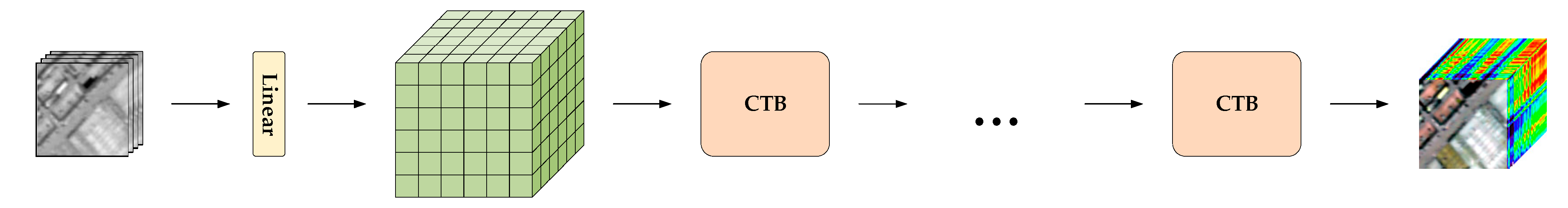
3.2. Network Architecture
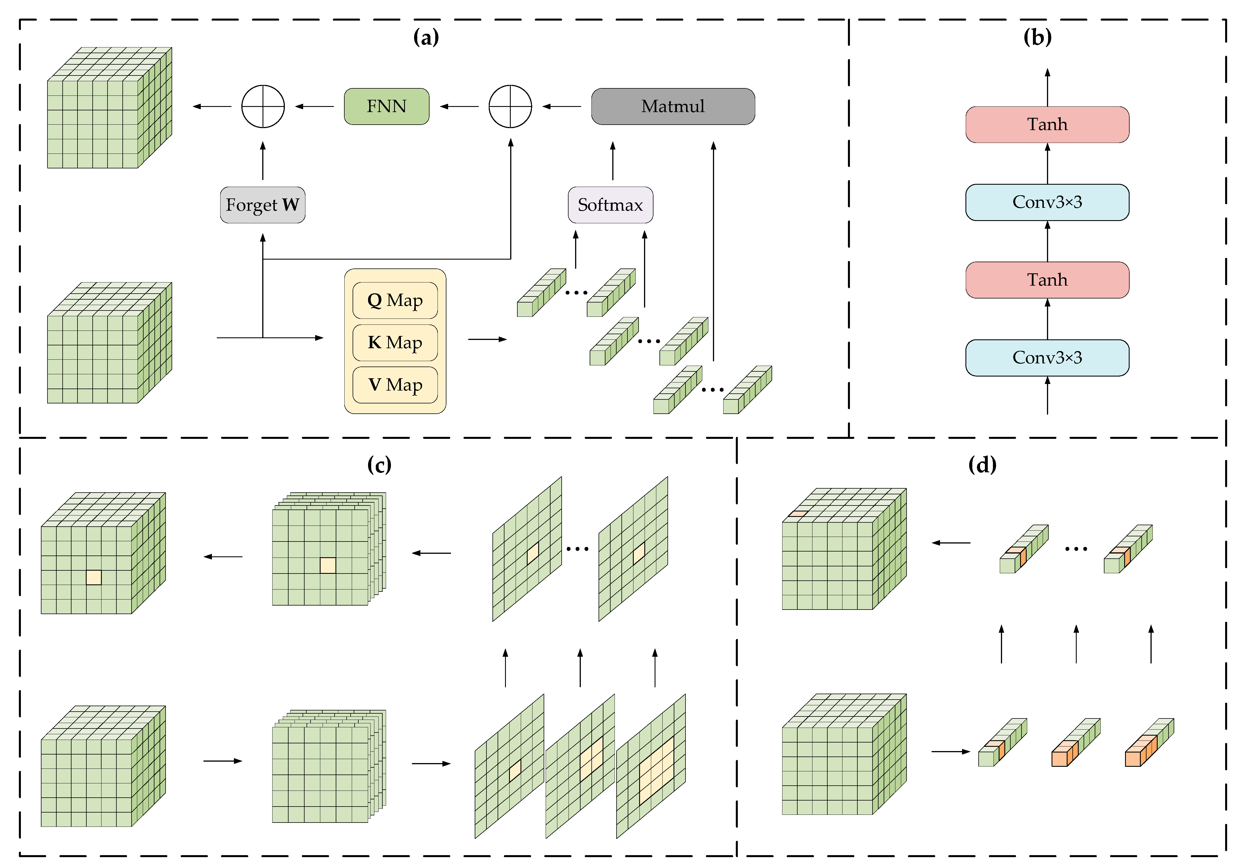
3.3. CTB Structure
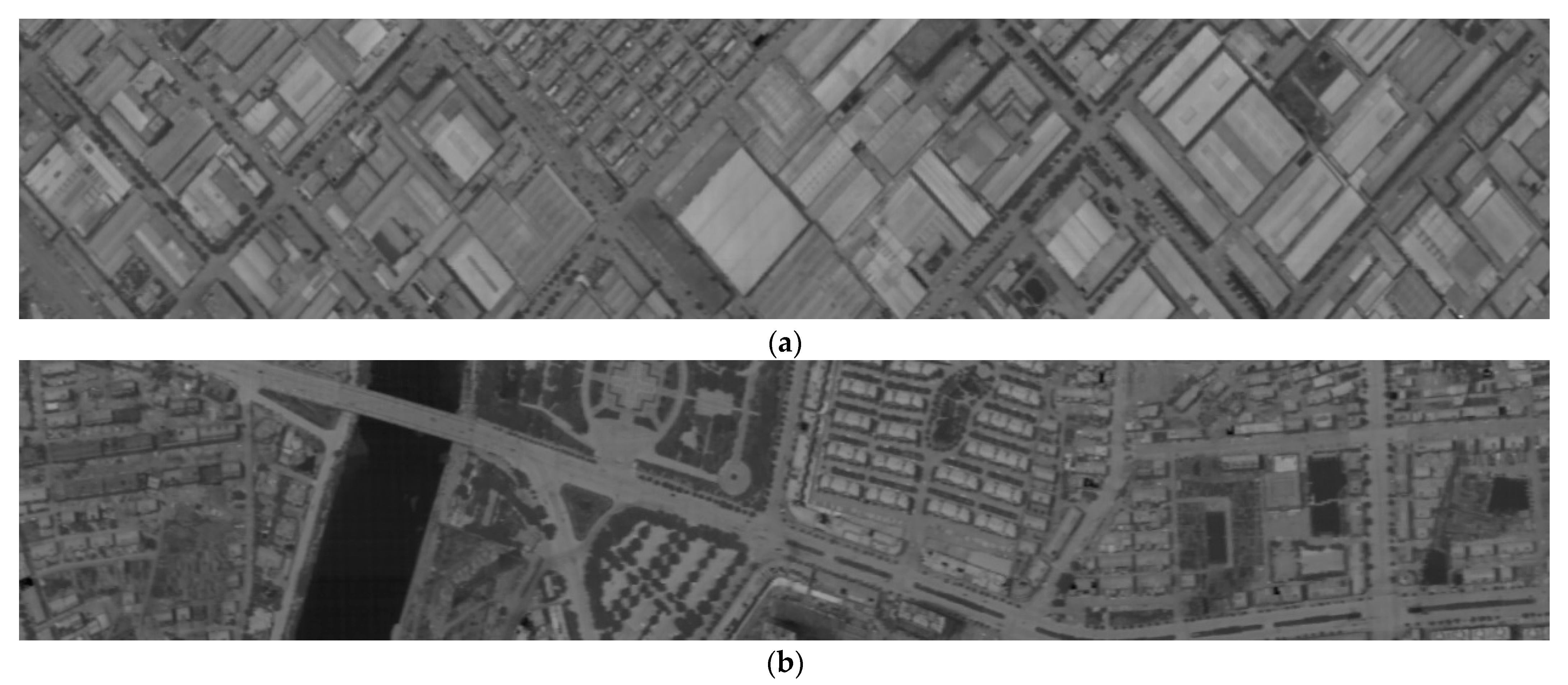
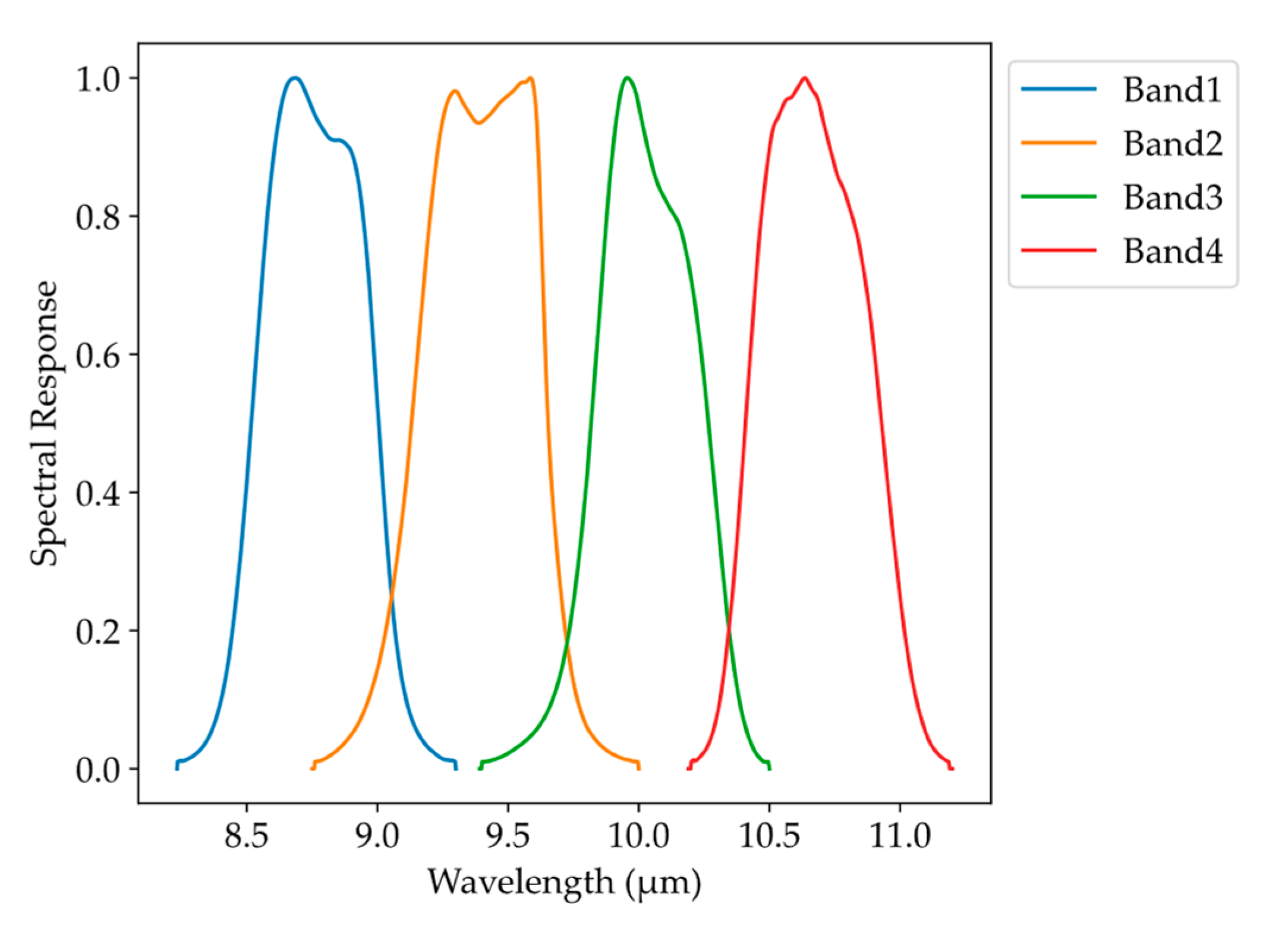
4. Dataset
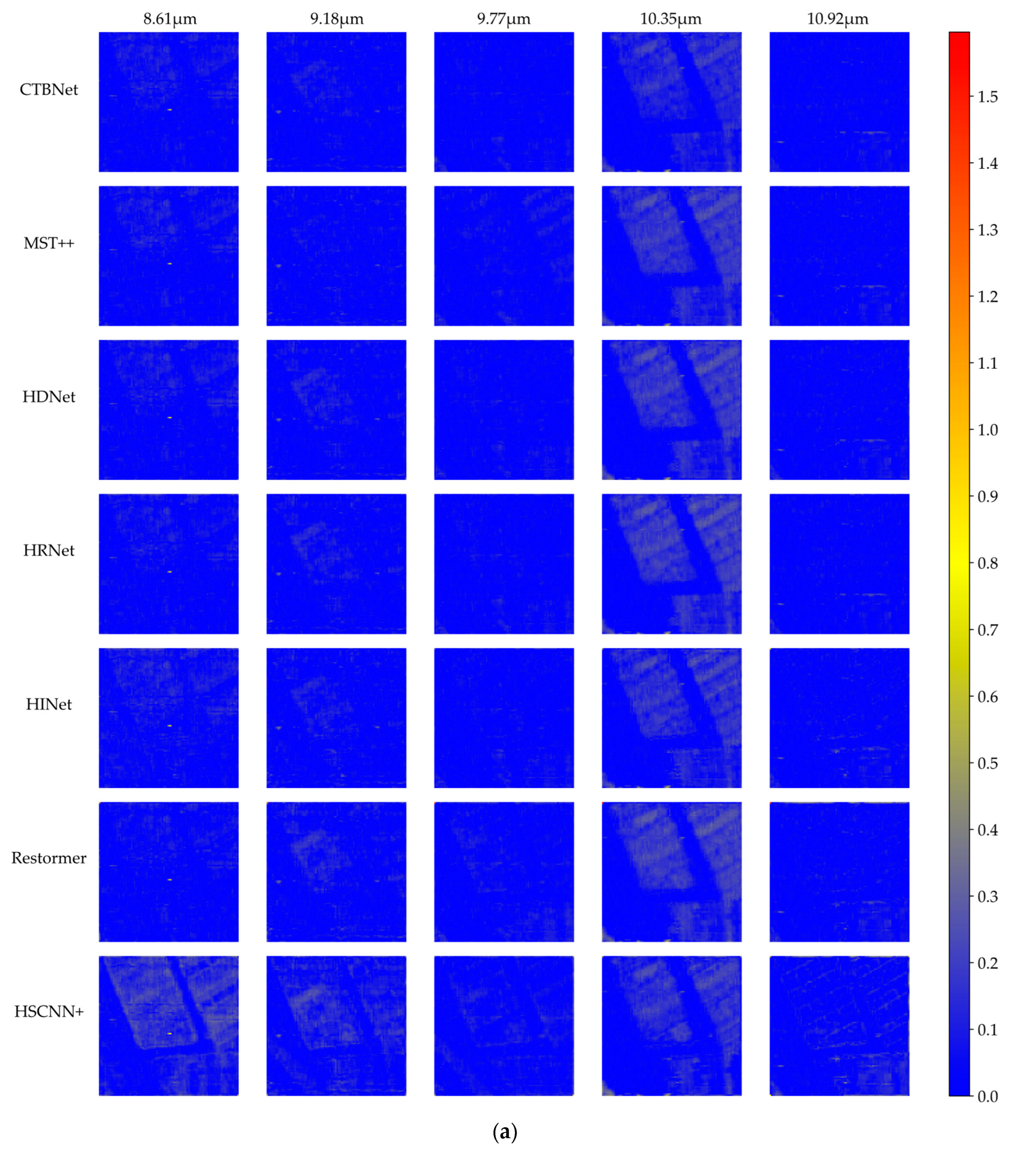
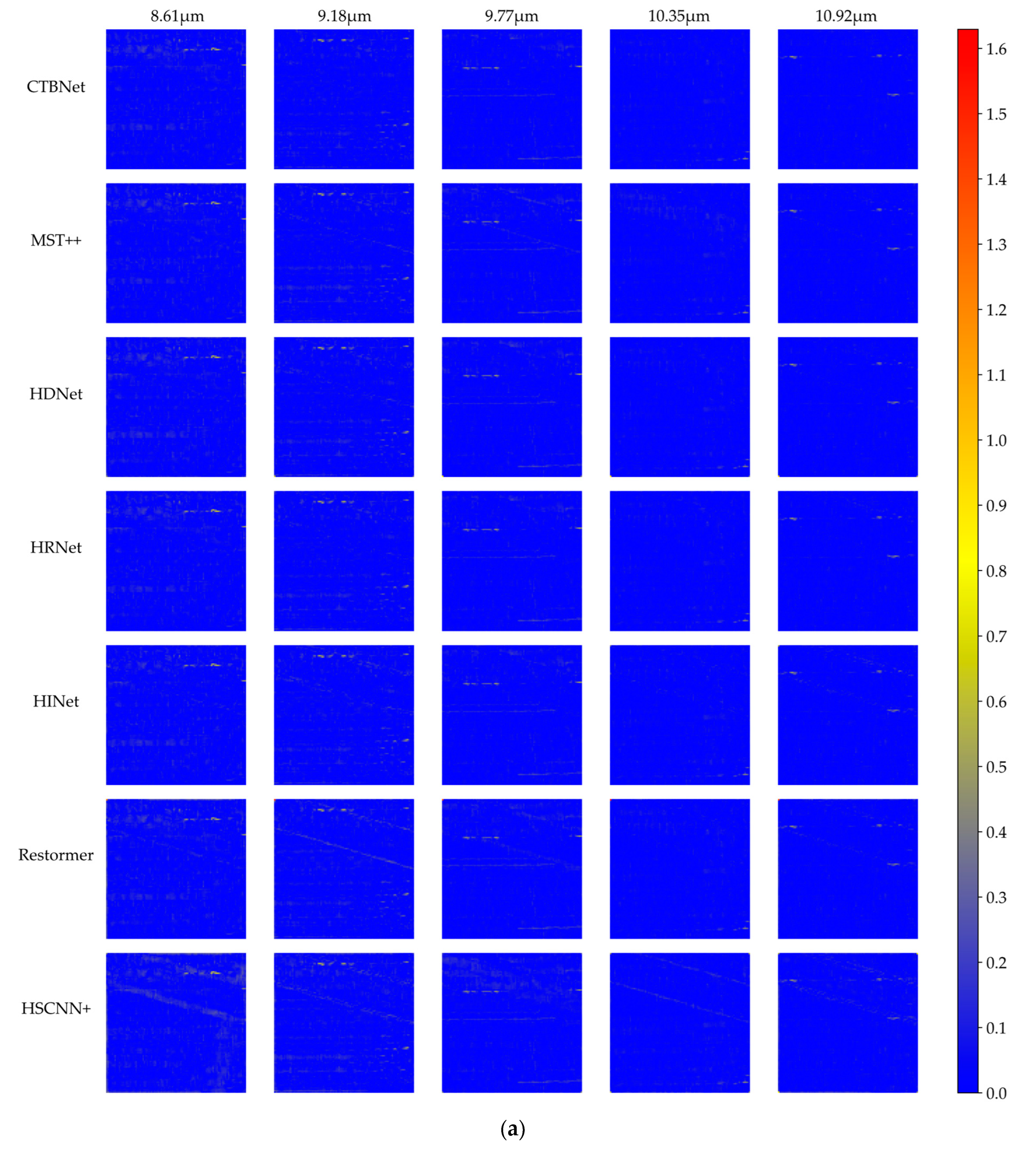
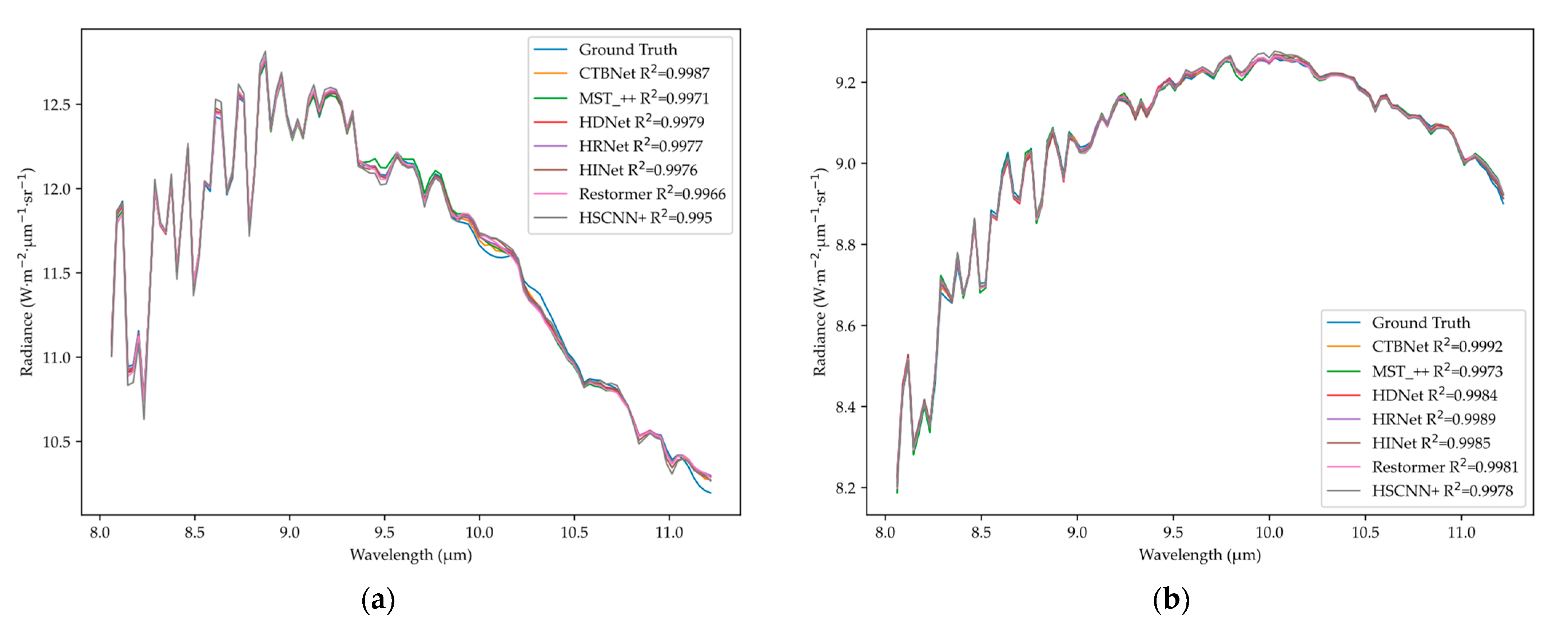
5. Results
6. Discussion
6.1. Ablation Study
6.2. Sensitivity Analysis
6.2.1. Influence of Instrument Noise
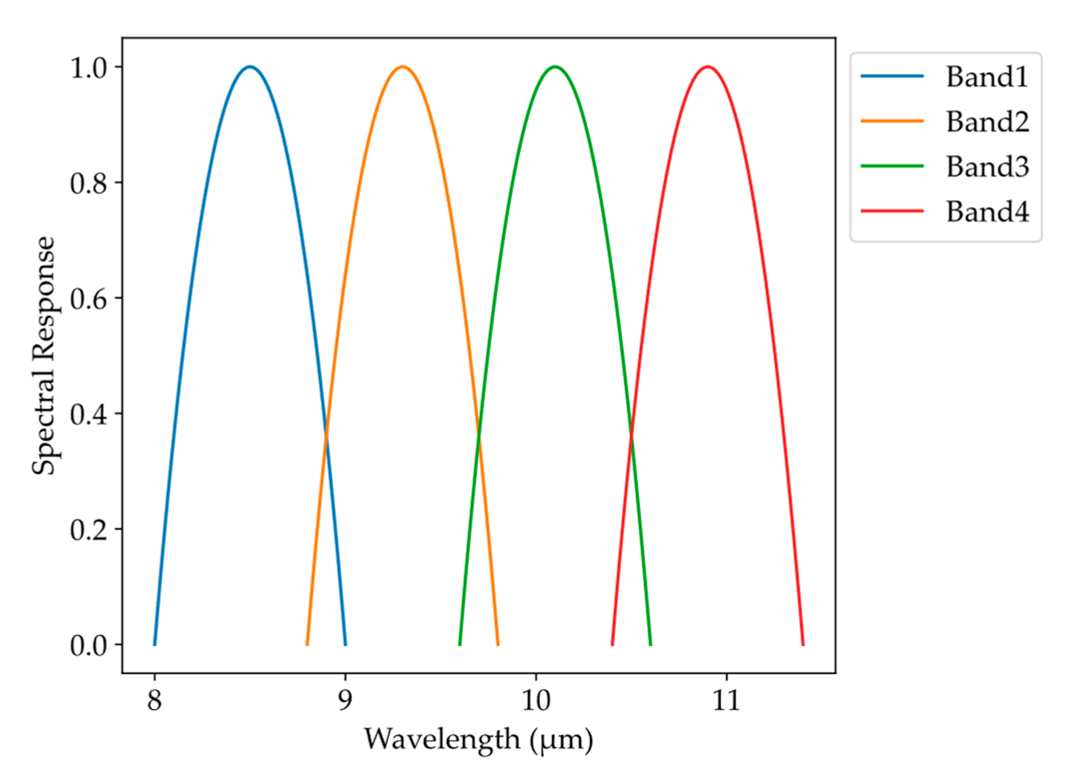
6.2.2. Influence of Spectral Response Function
7. Conclusions
Author Contributions
Funding
Data Availability Statement
Conflicts of Interest
References
- Li, Z.-L.; Wu, H.; Duan, S.-B.; Zhao, W.; Ren, H.; Liu, X.; Leng, P.; Tang, R.; Ye, X.; Zhu, J.; et al. Satellite Remote Sensing of Global Land Surface Temperature: Definition, Methods, Products, and Applications. Rev. Geophys. 2023, 61, 1–77. [Google Scholar] [CrossRef]
- Zhu, X.; Cao, L.; Wang, S.; Gao, L.; Zhong, Y. Anomaly Detection in Airborne Fourier Transform Thermal Infrared Spectrometer Images Based on Emissivity and a Segmented Low-Rank Prior. Remote Sens. 2021, 13, 754. [Google Scholar] [CrossRef]
- Liu, X.; Li, Z.-L.; Li, Y.; Wu, H.; Zhou, C.; Si, M.; Leng, P.; Duan, S.-B.; Yang, P.; Wu, W.; et al. Local temperature responses to actual land cover changes present significant latitudinal variability and asymmetry. Sci. Bull. 2023, 68, 2849–2861. [Google Scholar] [CrossRef] [PubMed]
- Zhang, D.; Zhu, Z.; Zhang, L.; Sun, X.; Zhang, Z.; Zhang, W.; Li, X.; Zhu, Q. Response of Industrial Warm Drainage to Tide Revealed by Airborne and Sea Surface Observations. Remote Sens. 2023, 15, 205. [Google Scholar] [CrossRef]
- Wang, Y.; Chen, X.; Wang, F.; Song, M.; Yu, C. Meta-Learning Based Hyperspectral Target Detection Using Siamese Network. IEEE Trans. Geosci. Remote Sens. 2022, 60, 5527913. [Google Scholar] [CrossRef]
- Li, Y.; Li, Z.-L.; Wu, H.; Zhou, C.; Liu, X.; Leng, P.; Yang, P.; Wu, W.; Tang, R.; Shang, G.-F.; et al. Biophysical impacts of earth greening can substantially mitigate regional land surface temperature warming. Nat. Commun. 2023, 14, 121. [Google Scholar] [CrossRef] [PubMed]
- Maes, W.H.; Steppe, K. Perspectives for Remote Sensing with Unmanned Aerial Vehicles in Precision Agriculture. Trends Plant Sci. 2019, 24, 152–164. [Google Scholar] [CrossRef] [PubMed]
- Kuai, L.; Kalashnikova, O.V.; Hopkins, F.M.; Hulley, G.C.; Lee, H.; Garay, M.J.; Duren, R.M.; Worden, J.R.; Hook, S.J. Quantification of Ammonia Emissions with High Spatial Resolution Thermal Infrared Observations from the Hyperspectral Thermal Emission Spectrometer (HyTES) Airborne Instrument. IEEE J. Sel. Top. Appl. Earth Observ. Remote Sens. 2019, 12, 4798–4812. [Google Scholar] [CrossRef]
- Wang, Y.; Zhu, Q.; Ma, H.; Yu, H. A Hybrid Gray Wolf Optimizer for Hyperspectral Image Band Selection. IEEE Trans. Geosci. Remote Sens. 2022, 60, 5527713. [Google Scholar] [CrossRef]
- Liu, H.; Wu, K.; Xu, H.; Xu, Y. Lithology Classification Using TASI Thermal Infrared Hyperspectral Data with Convolutional Neural Networks. Remote Sens. 2021, 13, 3117. [Google Scholar] [CrossRef]
- Fahlen, J.E.; Brodrick, P.G.; Thompson, D.R.; Herman, R.L.; Hulley, G.; Cawse-Nicholson, K.; Green, R.O.; Green, J.J.; Hook, S.J.; Miller, C.E. Joint VSWIR-TIR retrievals of earth's surface and atmosphere. Remote Sens. Environ. 2021, 267, 112727. [Google Scholar] [CrossRef]
- Black, M.; Riley, T.R.; Ferrier, G.; Fleming, A.H.; Fretwell, P.T. Automated lithological mapping using airborne hyperspectral thermal infrared data: A case study from Anchorage Island, Antarctica. Remote Sens. Environ. 2016, 176, 225–241. [Google Scholar] [CrossRef]
- Wang, Y.; Chen, X.; Zhao, E.; Song, M. Self-Supervised Spectral-Level Contrastive Learning for Hyperspectral Target Detection. IEEE Trans. Geosci. Remote Sens. 2023, 61, 5510515. [Google Scholar] [CrossRef]
- Koz, A.; Efe, U. Geometric- and Optimization-Based Registration Methods for Long-Wave Infrared Hyperspectral Images. Remote Sens. 2021, 13, 2465. [Google Scholar] [CrossRef]
- Qi, M.; Cao, L.; Zhao, Y.; Jia, F.; Song, S.; He, X.; Yan, X.; Huang, L.; Yin, Z. Quantitative Analysis of Mixed Minerals with Finite Phase Using Thermal Infrared Hyperspectral Technology. Materials 2023, 16, 2743. [Google Scholar] [CrossRef] [PubMed]
- Li, T.; Gu, Y. Progressive Spatial–Spectral Joint Network for Hyperspectral Image Reconstruction. IEEE Trans. Geosci. Remote Sens. 2022, 60, 5507414. [Google Scholar] [CrossRef]
- Gerhards, M.; Schlerf, M.; Mallick, K.; Udelhoven, T. Challenges and Future Perspectives of Multi-/Hyperspectral Thermal Infrared Remote Sensing for Crop Water-Stress Detection: A Review. Remote Sens. 2019, 11, 1240. [Google Scholar] [CrossRef]
- Wang, Y.; Wang, L.; Yu, C.; Zhao, E.; Song, M.; Wen, C.-H.; Chang, C.-I. Constrained-Target Band Selection for Multiple-Target Detection. IEEE Trans. Geosci. Remote Sens. 2019, 57, 6079–6103. [Google Scholar] [CrossRef]
- Zhang, J.; Su, R.; Fu, Q.; Ren, W.; Heide, F.; Nie, Y. A survey on computational spectral reconstruction methods from RGB to hyperspectral imaging. Sci. Rep. 2022, 12, 11905. [Google Scholar] [CrossRef] [PubMed]
- Zhao, E.; Gao, C.; Han, Q.; Yao, Y.; Wang, Y.; Yu, C.; Yu, H. An Operational Land Surface Temperature Retrieval Methodology for Chinese Second-Generation Huanjing Disaster Monitoring Satellite Data. IEEE J. Sel. Top. Appl. Earth Observ. Remote Sens. 2022, 15, 1283–1292. [Google Scholar] [CrossRef]
- Gade, R.; Moeslund, T.B. Thermal cameras and applications: A survey. Mach. Vis. Appl. 2014, 25, 245–262. [Google Scholar] [CrossRef]
- Zou, C.; Wei, M. Cluster-based deep convolutional networks for spectral reconstruction from RGB images. Neurocomputing 2021, 464, 342–351. [Google Scholar] [CrossRef]
- Huang, L.; Luo, R.; Liu, X.; Hao, X. Spectral imaging with deep learning. Light-Sci. Appl. 2022, 11, 61. [Google Scholar] [CrossRef] [PubMed]
- Qu, Q.; Pan, B.; Xu, X.; Li, T.; Shi, Z. Unmixing Guided Unsupervised Network for RGB Spectral Super-Resolution. IEEE Trans. Image Process. 2023, 32, 4856–4867. [Google Scholar] [CrossRef] [PubMed]
- Fu, Y.; Zheng, Y.; Zhang, L.; Huang, H. Spectral Reflectance Recovery From a Single RGB Image. IEEE Trans. Comput. Imaging 2018, 4, 382–394. [Google Scholar] [CrossRef]
- Fotiadou, K.; Tsagkatakis, G.; Tsakalides, P. Spectral Super Resolution of Hyperspectral Images via Coupled Dictionary Learning. IEEE Trans. Geosci. Remote Sens. 2019, 57, 2777–2797. [Google Scholar] [CrossRef]
- Zhao, J.; Kechasov, D.; Rewald, B.; Bodner, G.; Verheul, M.; Clarke, N.; Clarke, J.L. Deep Learning in Hyperspectral Image Reconstruction from Single RGB images-A Case Study on Tomato Quality Parameters. Remote Sens. 2020, 12, 3258. [Google Scholar] [CrossRef]
- Miao, X.; Yuan, X.; Pu, Y.; Athitsos, V. lambda-Net: Reconstruct Hyperspectral Images From a Snapshot Measurement. In Proceedings of the 2019 IEEE/CVF International Conference on Computer Vision (ICCV), Seoul, Republic of Korea, 27 October–2 November 2019. [Google Scholar]
- Zhu, L.; Wu, J.; Biao, W.; Liao, Y.; Gu, D. SpectralMAE: Spectral Masked Autoencoder for Hyperspectral Remote Sensing Image Reconstruction. Sensors 2023, 23, 3728. [Google Scholar] [CrossRef] [PubMed]
- Han, X.; Zhang, H.; Xue, J.H.; Sun, W. A Spectral–Spatial Jointed Spectral Super-Resolution and Its Application to HJ-1A Satellite Images. IEEE Geosci. Remote Sens. Lett. 2022, 19, 5505905. [Google Scholar] [CrossRef]
- Vaswani, A.; Shazeer, N.; Parmar, N.; Uszkoreit, J.; Jones, L.; Gomez, A.N.; Kaiser, L.; Polosukhin, I. Attention is All you Need. In Proceedings of the Neural Information Processing Systems, Long Beach, CA, USA, 4–9 December 2017. [Google Scholar]
- Rogers, A.; Kovaleva, O.; Rumshisky, A. A Primer in BERTology: What We Know About How BERT Works. Trans. Assoc. Comput. Linguist. 2020, 8, 842–866. [Google Scholar] [CrossRef]
- Liu, Z.; Lin, Y.; Cao, Y.; Hu, H.; Wei, Y.; Zhang, Z.; Lin, S.; Guo, B. Swin Transformer: Hierarchical Vision Transformer Using Shifted Windows. In Proceedings of the IEEE/CVF International Conference on Computer Vision (ICCV), Montreal, QC, Canada, 10–17 October 2021. [Google Scholar]
- Du, D.; Gu, Y.; Liu, T.; Li, X. Spectral Reconstruction from Satellite Multispectral Imagery Using Convolution and Transformer Joint Network. IEEE Trans. Geosci. Remote Sens. 2023, 61, 5515015. [Google Scholar] [CrossRef]
- Carion, N.; Massa, F.; Synnaeve, G.; Usunier, N.; Kirillov, A.; Zagoruyko, S. End-to-End Object Detection with Transformers. In Proceedings of the Computer Vision—ECCV 2020: 16th European Conference, Glasgow, UK, 23–28 August 2020. [Google Scholar]
- Chen, K.; Zou, Z.; Shi, Z. Building Extraction from Remote Sensing Images with Sparse Token Transformers. Remote Sens. 2021, 13, 4441. [Google Scholar] [CrossRef]
- Cai, Y.; Lin, J.; Lin, Z.; Wang, H.; Zhang, Y.; Pfister, H.; Timofte, R.; Gool, L.V. MST++: Multi-stage Spectral-wise Transformer for Efficient Spectral Reconstruction. In Proceedings of the 2022 IEEE/CVF Conference on Computer Vision and Pattern Recognition Workshops (CVPRW), New Orleans, LA, USA, 19–20 June 2022. [Google Scholar]
- Zhao, Y.; Po, L.-M.; Yan, Q.; Liu, W.; Lin, T. Hierarchical Regression Network for Spectral Reconstruction from RGB Images. In Proceedings of the 2020 IEEE/CVF Conference on Computer Vision and Pattern Recognition Workshops (CVPRW), Seattle, WA, USA, 14–19 June 2020. [Google Scholar]
- Shi, Z.; Chen, C.; Xiong, Z.; Liu, D.; Wu, F. HSCNN+: Advanced CNN-Based Hyperspectral Recovery from RGB Images. In Proceedings of the 2018 IEEE/CVF Conference on Computer Vision and Pattern Recognition Workshops (CVPRW), Salt Lake City, UT, USA, 18–22 June 2018. [Google Scholar]
- Hu, X.; Cai, Y.; Lin, J.; Wang, H.; Yuan, X.; Zhang, Y.; Timofte, R.; Gool, L.V. HDNet: High-resolution Dual-domain Learning for Spectral Compressive Imaging. In Proceedings of the 2022 IEEE/CVF Conference on Computer Vision and Pattern Recognition (CVPR), New Orleans, LA, USA, 18–24 June 2022. [Google Scholar]
- Chen, L.; Lu, X.; Zhang, J.; Chu, X.; Chen, C. HINet: Half Instance Normalization Network for Image Restoration. In Proceedings of the 2021 IEEE/CVF Conference on Computer Vision and Pattern Recognition (CVPR), Online, 19–25 June 2021. [Google Scholar]
- Zamir, S.W.; Arora, A.; Khan, S.; Hayat, M.; Khan, F.S.; Yang, M.-H. Restormer: Efficient Transformer for High-Resolution Image Restoration. In Proceedings of the 2022 IEEE/CVF Conference on Computer Vision and Pattern Recognition (CVPR), New Orleans, LA, USA, 18–24 June 2022. [Google Scholar]
- Sun, W.; Ren, K.; Meng, X.; Yang, G.; Xiao, C.; Peng, J.; Huang, J. MLR-DBPFN: A Multi-Scale Low Rank Deep Back Projection Fusion Network for Anti-Noise Hyperspectral and Multispectral Image Fusion. IEEE Trans. Geosci. Remote Sens. 2022, 60, 5522914. [Google Scholar] [CrossRef]
- Zhang, H.; Cai, J.; He, W.; Shen, H.; Zhang, L. Double Low-Rank Matrix Decomposition for Hyperspectral Image Denoising and Destriping. IEEE Trans. Geosci. Remote Sens. 2022, 60, 5502619. [Google Scholar] [CrossRef]
- Zhuang, L.; Ng, M.K.; Liu, Y. Cross-Track Illumination Correction for Hyperspectral Pushbroom Sensor Images Using Low-Rank and Sparse Representations. IEEE Trans. Geosci. Remote Sens. 2023, 61, 5502117. [Google Scholar] [CrossRef]
- Capelle, V.; Hartmann, J.-M. Use of hyperspectral sounders to retrieve daytime sea-surface temperature from mid-infrared radiances: Application to IASI. Remote Sens. Environ. 2022, 280, 113171. [Google Scholar] [CrossRef]
- Lan, X.; Zhao, E.; Leng, P.; Li, Z.-L.; Labed, J.; Nerry, F.; Zhang, X.; Shang, G. Alternative Physical Method for Retrieving Land Surface Temperatures from Hyperspectral Thermal Infrared Data: Application to IASI Observations. IEEE Trans. Geosci. Remote Sens. 2022, 60, 1–12. [Google Scholar] [CrossRef]
- Ricciardelli, E.; Paola, F.; Cimini, D.; Larosa, S.; Mastro, P.; Masiello, G.; Serio, C.; Hultberg, T.; August, T.; Romano, F. A Feedforward Neural Network Approach for the Detection of Optically Thin Cirrus From IASI-NG. IEEE Trans. Geosci. Remote Sens. 2023, 61, 4104217. [Google Scholar] [CrossRef]


| PSNR (dB) | SSIM | SAM (rad) | RMSE (K) | MRAE | |
|---|---|---|---|---|---|
| MST++ | 60.93172 | 0.98797 | 0.00091 | 0.31442 | 0.00068 |
| HRNet | 61.37429 | 0.98842 | 0.00085 | 0.29734 | 0.00063 |
| HSCNN+ | 59.1247 | 0.98611 | 0.00109 | 0.4063 | 0.00083 |
| Restormer | 60.14287 | 0.98824 | 0.00095 | 0.35053 | 0.00071 |
| HDNet | 61.058 | 0.98855 | 0.00088 | 0.30924 | 0.00065 |
| HINet | 60.97999 | 0.9879 | 0.00089 | 0.30969 | 0.00066 |
| CTBNet | 61.48676 | 0.98864 | 0.00084 | 0.29338 | 0.00062 |
| PSNR (dB) | SSIM | SAM (rad) | RMSE (K) | MRAE | |
|---|---|---|---|---|---|
| CTBNet | 61.48676 | 0.98864 | 0.00084 | 0.29338 | 0.00062 |
| New-Attention | 59.93308 | 0.98728 | 0.00093 | 0.36361 | 0.00074 |
| Nom-Attention | 61.42158 | 0.98854 | 0.00085 | 0.29546 | 0.00063 |
| Nom-Transformer | 57.79278 | 0.98686 | 0.00098 | 0.46456 | 0.00109 |
| PSNR (dB) | SSIM | SAM (rad) | RMSE (K) | MRAE | |
|---|---|---|---|---|---|
| Without_noise | 61.48676 | 0.98864 | 0.00084 | 0.29338 | 0.00062 |
| With_noise | 61.11164 | 0.98793 | 0.00088 | 0.30397 | 0.00066 |
| PSNR (dB) | SSIM | SAM (rad) | RMSE (K) | MRAE | |
|---|---|---|---|---|---|
| Ideal data | 61.48676 | 0.98864 | 0.00084 | 0.29338 | 0.00062 |
| MODIS data | 61.24813 | 0.98838 | 0.00089 | 0.31294 | 0.00065 |
Disclaimer/Publisher’s Note: The statements, opinions and data contained in all publications are solely those of the individual author(s) and contributor(s) and not of MDPI and/or the editor(s). MDPI and/or the editor(s) disclaim responsibility for any injury to people or property resulting from any ideas, methods, instructions or products referred to in the content. |
© 2024 by the authors. Licensee MDPI, Basel, Switzerland. This article is an open access article distributed under the terms and conditions of the Creative Commons Attribution (CC BY) license (https://creativecommons.org/licenses/by/4.0/).
Share and Cite
Zhao, E.; Qu, N.; Wang, Y.; Gao, C. Spectral Reconstruction from Thermal Infrared Multispectral Image Using Convolutional Neural Network and Transformer Joint Network. Remote Sens. 2024, 16, 1284. https://doi.org/10.3390/rs16071284
Zhao E, Qu N, Wang Y, Gao C. Spectral Reconstruction from Thermal Infrared Multispectral Image Using Convolutional Neural Network and Transformer Joint Network. Remote Sensing. 2024; 16(7):1284. https://doi.org/10.3390/rs16071284
Chicago/Turabian StyleZhao, Enyu, Nianxin Qu, Yulei Wang, and Caixia Gao. 2024. "Spectral Reconstruction from Thermal Infrared Multispectral Image Using Convolutional Neural Network and Transformer Joint Network" Remote Sensing 16, no. 7: 1284. https://doi.org/10.3390/rs16071284