Abstract
When there are dynamic obstacles in the environment, it is difficult for traditional path-generation algorithms to achieve desired obstacle-avoidance results. To solve this problem, we propose a robot navigation control method based on SAC (Soft Actor-Critic) Deep Reinforcement Learning. Firstly, we use a fast path-generation algorithm to control the robot to generate expert trajectories when the robot encounters danger as well as when it approaches a target, and we combine SAC reinforcement learning with imitation learning based on expert trajectories to improve the safety of training. Then, for the hybrid data consisting of agent data and expert data, we use an improved prioritized experience replay method to improve the learning efficiency of the policies. Finally, we introduce RNN (Recurrent Neural Network) units into the network structure of the SAC Deep Reinforcement-Learning navigation policy to improve the agent’s transfer inference ability in a new environment and obstacle-avoidance ability in dynamic environments. Through simulation and practical experiments, it is fully verified that our method has a higher training efficiency and navigation success rate compared to state-of-the-art reinforcement-learning algorithms, which further enhances the obstacle-avoidance capability of the robot system.
1. Introduction
The traditional deterministic model-based path-generation algorithm relies heavily on sensor data, and when the sensor’s field of view is more seriously obscured by obstacles in the environment, the above path-generation algorithm will make it difficult for the robot to achieve the desired obstacle-avoidance results []. In order to solve this problem, we carried out research on robot navigation control methods based on Soft Actor-Critic deep reinforcement learning using LiDAR.
Deep reinforcement learning is an algorithm that integrates deep neural networks and reinforcement learning to solve complex decision-making tasks []. With the fitting ability of deep neural networks, it solves the mapping from observed features to strategy and value functions, and at the same time, it uses reinforcement-learning algorithms to define the optimization problem and optimization objective and continuously improves the decision-making ability of the agent in the process of interacting with information from the environment. The important metrics to be considered for training robot navigation policies using Deep Reinforcement-Learning methods include (i) sampling efficiency, i.e., how to train the agent’s navigation ability at a faster rate with limited data; (ii) safety—since the physical robot cannot collide with the environment randomly, as it can in the simulation environment, the algorithm needs to learn in a safe situation; and (iii) transfer inference ability—since there are usually dynamic objects in the environment, the agent also needs some transfer inference ability to accomplish the desired dynamic obstacle avoidance. The main innovations of this study are as follows:
- (1)
- We use fast path-generation algorithm to control the robot to generate expert trajectories, combine SAC reinforcement learning with imitation learning based on expert trajectories to solve the problem of the poor navigation ability of the agent in the initial state, and improve the training safety and convergence speed of reinforcement learning.
- (2)
- Considering that the priority of expert trajectory data is higher than that of agent trajectory data, we improve the priority calculation method on the basis of the TD-error (time-difference error) priority replay technique, which improves the utilization efficiency of the data in the experience replay pool.
- (3)
- We introduced an RNN to improve the obstacle-avoidance ability of SAC navigation policy in a dynamic environment.
2. Related Work
Most approaches to reinforcement learning belong to model-free methods, which can be further categorized into value-based such as Q-learning [], SARSA [], and so on. However, these traditional reinforcement-learning methods can only be applied to low-dimensional simple tasks. With the rapid development of deep learning, there have been attempts to combine deep learning with reinforcement learning to deal with more complex tasks, which are called Deep Reinforcement-Learning (DRL) methods. DRL uses deep neural networks as nonlinear approximators to fit value functions, policies, or models, which can solve the bottleneck problem of traditional reinforcement learning that is limited to state dimensions and continuous spaces. Deep Q-network (DQN) [] utilizes neural networks to replace the tables that record state action values in Q-learning, which can be used in discrete action spaces and trained in an offline manner, but the simultaneous presence of an offline policy, nonlinear function approximation, and self-starting make the Q-learning algorithm difficult to converge. Various improved versions have emerged to address the shortcomings of DQN, e.g., Double DQN [] builds on DQN by first using an evaluation network to determine the action and then using a target network to determine the value of the state action, which prevents uneven overestimation in DQN. Dueling DQN [] adopts the structure of dyadic network after the neural network outputs the state value and the advantage value of the action, and the corresponding Q value can be obtained by adding the state value and the advantage value. This method can improve the convergence speed and enhance the learning effect. Rainbow [] combines multiple improvement methods of DQN to achieve a better effect than a single improvement.
In addition to value-based reinforcement-learning methods like DQN, another large class of methods is directly policy-based methods, which can directly pick action outputs in a continuous space. Trust Region Policy Optimization (TRPO) uses the largest possible learning step to increase the convergence speed and introduces constraints during the policy optimization process to ensure that the new policy is better than the old one. Proximal Policy Optimization (PPO) [], proposed by DeepMind, is based on TRPO and adds KL scattering constraints into the objective function to simplify the computation process, which has achieved good results in continuous control. OpenAI has also proposed its own version of PPO [], which uses a first-order approach and a few tricks to approximate strict mathematical constraints as closely as possible, further eliminating the computation of KL dispersion and striking a good balance between expressive performance and generalization ability. In addition to the value-based and strategy frameworks, there is also Actor-Critic, a methodological framework that combines the two. DDPG (Deep Deterministic Policy Gradient) [,] can be used to output continuous actions, which combines the advantages of DQN to improve the stability and speed of algorithm convergence. SQL (Soft Q-learning) [] is an offline stochastic policy that targets maximum entropy and is based on an energy-expression-based policy; the algorithm expresses the optimal policy through a Boltzmann distribution, is insensitive to hyperparameters, and has excellent performance. After SQL, the authors further proposed the SAC (Soft Actor-Critic) [] framework, which consists of strategy iteration and strategy boosting, where the strategy is fixed during the iterative strategy evaluation, and then the Bellman equation containing entropy is used to update the Q-value until convergence. In the strategy boosting phase, minimizing the distance between the distribution of the strategy and the KL scattering based on the energy distribution is carried out to learn the strategy parameters, and the algorithm is easy to implement and has excellent performance and good robustness.
Currently, combining reinforcement learning with navigation policies for mobile robots is a research hotspot. Lei T et al. [] input depth camera images into a pre-trained convolutional neural network to obtain feature mappings and then input the feature mappings into a fully connected layer to obtain Q-values to train a robot for sustained collision-free motion in a corridor environment. Jaradat et al. [] proposed a Q-learning reinforcement-learning path-navigation algorithm due to its use of discrete distances and angles to classify the environment, resulting in a less-flexible robot, and the effectiveness of the algorithm is heavily dependent on the quality of the designed state, which has a strong learning ability in simple environments but is indeed difficult to adapt to complex environments. Anthony et al. [] proposed a reinforcement-learning navigation policy combined with the traditional path planning method Probabilistic Roadmaps (PRMs), where the PRM (or A*) algorithm is utilized globally to scavenge for optimal paths, and then the reinforcement-learning policy executes the small goals one by one, which allows for navigation planning over a larger area. Safety is an important factor to consider when applying reinforcement learning to real-world domains such as robot navigation policies and robotic arm operation. Q. Yang et al. [] proposed a worst-case secure SAC reinforcement-learning method considering the distribution of security costs, which possesses better risk control performance compared to the expectation-based secure reinforcement-learning method. Gal Dalal et al. [] added a linear safety layer to the continuous action output of DDPG reinforcement learning, but the method requires the high accuracy of the pre-trained safety layer, and the prediction cost needs to be expressed as a linear relationship. A. Stooke et al. [] viewed the traditional Lagrangian method applied to safety reinforcement learning as an I-session; then, they added a P-session and a D-session to reduce oscillations and verified that the algorithm could achieve better results in the safety gym environment, but the method still could not directly control and guarantee the safety of the agent training.
The abovementioned reinforcement-learning methods applied to the robot navigation process have problems such as low navigation efficiency, lack of safety considerations, and no reduction of human involvement. To solve the above problems, we carried out a robot navigation control method based on SAC deep reinforcement learning.
3. SAC Reinforcement-Learning Navigation Policy Incorporating Expert Data-Based Imitation Learning
When training a robot (agent) is using reinforcement learning, only two-dimensional position information is usually considered, and less consideration is given to the robot’s pose information, which is often very important in real applications when the robot reaches the target point. In a reinforcement-learning navigation task, introducing attitude constraints at the target point would bring about greater training difficulty. In the early stages of training when the robot is close to the target point, the actions output from the reinforcement-learning method often cause the robot to miss the target point, oscillate around the target point, or arrive at the target point at a large speed, resulting in a reduction in training effectiveness and safety. This is shown in Figure 1.
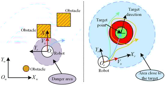
Figure 1.
Reinforcement-learning navigation policy incorporating expert data-based imitation learning. In Figure 1, the blue region in the right circle is the region close to the target point, the blue trajectory is the optimal trajectory obtained by solving, the green trajectory is close to the target point but eventually far away, the yellow trajectory is the case of cycling or oscillating near the target point, and the red region indicates the dangerous region.
Considering the above, we use an analytic approach to quickly and accurately compute the optimal trajectory along which to reach the target point, allowing the experience replay pool to contain more successfully sampled data. In addition, utilizing actions close to the target to train the action policy results in a better way for the robot to reach the target point and in a better overall action effect of the agent, and it also improves the sampling efficiency of the training. When the robot is in a dangerous area, the robot is controlled to “extrication” using a fast path-generation algorithm, which is provided directly by the ROS (Robot Operating System) navigation package and is a fusion of the traditional A* and DWA algorithms [], so it will not be introduced here. The data generated by the above fast path-generation algorithm are recorded as expert data, and the blue trajectory in Figure 1 is the expert trajectory for “extrication”, and when it is out of the danger zone, the intervention is ended and is changed to the agent method to control the robot movement. In Figure 1, the left side of the figure represents the use of an expert method to help the robot get out of trouble and avoid obstacles, and the right side of the figure represents the situation after the robot gets out of trouble, when the agent takes over and controls the robot to reach the goal point quickly.
For ease of description, we call the method of controlling the robot’s “extrication” using traditional A* and DWA fusion algorithms an expert method, and the collected data are called expert data. The method of using reinforcement learning to control the robot’s motion is called the agent method, and the collected data are called agent data. Both the data collected by the expert method and the agent method are stored in the experience pool for offline training, and the data in the experience pool are played back using an improved prioritized experience calculation method. The offline SAC reinforcement-learning method is used to train the agent, and the overall navigation policy flow of this study is shown in Figure 2.
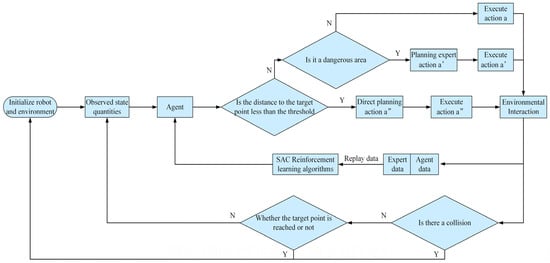
Figure 2.
The overall navigation policy process for this study.
In Figure 2, “a” denotes the action performed by the agent to control the robot. a′ and a″ denote the actions performed by the robot to control the robot when using the expert method to help the robot to perform extrication in different situations, respectively.
3.1. SAC Reinforcement-Learning Algorithm Based on Security Constraints
The core idea of the SAC algorithm is to learn the optimal action strategy through policy optimization and Q-function optimization. Specifically, the algorithm employs the dual optimization objectives of minimizing policy loss and Q-function loss. At each time step, it samples an action from the current state and computes a probability density function for that action. Then, the expectation of the product of that probability density function and the Q function is minimized to compute the policy loss. In calculating this expectation, the SAC algorithm introduces an entropy regularity term to ensure the explorability and stability of the policy, which aims to maximize the entropy of the policy, facilitates the exploration of more action space, and employs techniques such as goal networks and experience replay to improve the stability of the algorithm. The flowchart of the SAC algorithm is shown in Figure 3.
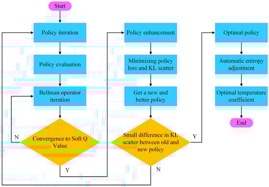
Figure 3.
Flowchart of SAC algorithm.
The optimal policy objective for SAC is as follows [,]:
where is the state, is the action, and is the time. is a temperature factor that regulates the randomness of the policy and is used to balance the relative importance between entropy and reward. When is large, the policy is biased toward randomness, while when is small, the policy tends to be deterministic. is the entropy, which indicates the randomness of the policy and is calculated as shown in Equation (2). is the discount factor, which indicates the length of time in the future to be considered.
Unlike the standard definitions of value function and action-value function, the soft Q-function and soft value function defined in SAC are shown in Equations (3) and (4), respectively.
where denotes the discounted future return of the agent under the condition of taking optimal action. denotes the state value function. Based on the above equation, the formula for the optimal policy can be directly introduced:
obeys the Boltzmann distribution of the energy model, where is negative energy and is used for normalization. The ideal sampling policy should follow the energy model above, but it is difficult to express it directly in terms of parameters, so the action policy constructs a neural network with parameter to sample the actions, where is a variable obeying a standard normal distribution. In order to make the policy approximate the optimal policy, the KL scattering method is utilized for constraints:
where is the empirical pool of data and denotes the Gaussian distribution. The optimization of the action policy is completed by following the gradient descent method for Equation (6), which guarantees convergence to the optimal policy [,]. The distance information of the robot from an obstacle during operation is converted into a cost value to keep the robot away from the obstacle during movement, improve navigation safety and ensure exploration performance:
where denotes the action-state cost value and denotes the distance threshold. is the closest distance of the robot to the obstacle measured by the LiDAR. and are two adjustable positive scale factors. is defined as described above, and in practice, it specifically refers to the size of the robot’s speed control command. For the above optimization problem with constraints, the Lagrange method is used to transform the constrained optimization problem into
To satisfy the constraints and for ease of computation, the PDO (Primal-Dual Optimization) method [] is used to solve and in Equation (8).
3.2. Training Process Based on Expert Methodology
Although the addition of a safety layer to the SAC navigation policy improves the safety of the training process, the cost expectation estimated by the neural network may not be completely accurate and may be affected by hyperparameters during the training process, resulting in a situation where unsafe collisions can still occur during the training process. In order to improve the training speed and safety of the SAC algorithm, we made the following improvements: the first one was dividing the area where the robot is located, and when the robot was in the dangerous area, the fast path-generation algorithm was used to help the robot to “extrication”, and at the same time, the expert data generated by the algorithm were collected. The second was using the fast path-generation algorithm to intervene with the agent when the robot’s distance and angle deviation from the target point were within a set threshold, so the robot could reach the target point quickly and obtain a higher reward value. The data from both cases are used as expert data for additional training using imitation learning in addition to the SAC method.
The agent consists of an Actor and a Critic, respectively, and is represented by a neural network as and , with characterizing the policy by outputting a Gaussian distribution, and outputting a numerical value characterizing the desired reward value of the state-action pair. Specifically, the Actor can output and through the neural network, then the action executed by agent under observation can be represented by sampling:
Let the action of the expert data be A, then the loss function for imitation learning can be constructed:
where is the size of the batch of expert data during offline training.
The training of Actor and Critic network parameters can be accomplished by using gradient descent for Equation (10). Using TD-error to update the value of the Critic for expert and agent data, assuming that the batch size of intelligent body data is , the error can be defined as follows:
where and denote the target value network and action network, respectively, and and are the corresponding network parameters.
3.3. An Improved Experience Replay Method Based on Mixed Data
The data in the experience replay pool contain both expert data and agent-generated data, which contain high-value training samples that have successfully reached the target point and collisions, while a large number of them are inefficient samples that have not reached the end point and have not collided. For agent training, expert data are more meaningful compared to agent data because expert data contain more prior information. The original prioritized experience replay (PER) algorithm uses the time-differential error as a priority, and the larger the TD-error value, the larger the gap between the estimated value of the state-action value and the target value, and the more it needs to be learned. The experience replay pool designed in this paper contains expert data in addition to data collected by agent, so it is necessary to increase the weight of expert data being sampled on this basis. Assuming that the agent’s action at moment is , while the expert’s action is , the Actor’s strategy is , and the Critic is denoted as . Then, the designed prioritization is calculated as follows:
where is a pre-determined positive number that guarantees that the weights are positive, and and are adjustable parameters characterizing the relative importance of action and value deviations. In the experience pool containing expert data and agent-collected data, the probability of data being sampled conforms to Equation (13).
The use of priority-based sampling changes the distribution of experience data in the replay pool and introduces bias into the estimation of the value function. Although biased Q-value estimation has no effect on reinforcement-learning consistency, it reduces the robustness of reinforcement-learning training. We eliminate this effect by assigning weights to the loss function with the help of importance sampling. The importance weights are calculated as:
where and is an adjustable parameter. Uniform sampling when means that importance sampling is not used, and when , it means that importance sampling is fully used. When updating the neural network, the loss function is multiplied by the importance weight and then updated using gradient descent. After each update to the neural network, the priority of the samples is updated.
4. Network Structure Design Based on Recurrent Neurons
4.1. Environmental Model
In the SAC reinforcement-learning-based navigation task, agent outputs speed commands based on the input state information to control the robot to interact with the environment, and finally, it can reach the specified target point without collision. The state information includes environment information, the robot’s own information, and target information. The environment model of the system is shown in Figure 4.
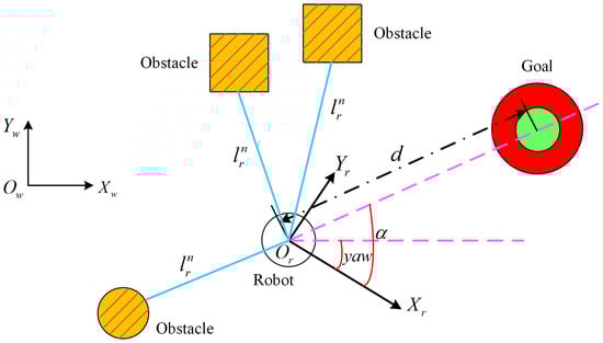
Figure 4.
System environment model.
In Figure 4, is the world coordinate system coordinates and is the robot coordinate system, where is the current velocity direction of the robot and is clockwise perpendicular to .
The environmental information that can be directly sensed by the robot through LIDAR is the distance from the robot to the obstacle; the self-information includes the robot’s position , and the target information includes the target point position as well as the robot’s distance and angle from the target point. The target information and describes the relative position information of the target point with respect to the robot, while the positions of the robot and the target point in the navigation process are usually described in the world coordinate system, so we need to transform the description of the target information in the world coordinate system to the robot coordinate system through coordinate transformation.
are the coordinates of the target point relative to the world coordinate system, which need to be transformed into the coordinates under the robot coordinate system when calculating the angle of pinch . From the robot’s pose , the target point can be transformed into the robot coordinate system to obtain the position of the target point under the robot coordinate system, which is calculated as shown in Equation (15).
The coordinates of the target point relative to the robot can be calculated from and :
The distance and relative angle between the robot and the target point can be calculated according to Equations (17) and (18).
Let denote the distance from the center of the robot to the obstacle measured by LiDAR. We normalize the distance information measured by the environment, the positional state information of the robot, the angle information of the target point, and the robot motion information , respectively. Then, the robot navigation task can be reduced to finding a function mapping , which maps all relevant information into decision commands to control the robot and leads it to move towards the target point without collision, which can be defined as:
We categorize all state information into two classes—LiDAR information is one class and other information combinations are the other class. The two classes of information are first extracted as features and , respectively, and then the extracted low-dimensional features and are jointly fed into the decision network, and the problem can be redefined as:
4.2. Reward Function Design
Only when the distance and the angular deviation between the robot and the target point are less than the set thresholds at the same time is the robot considered to have accomplished the planning goal, and the one-episode training is over. Assuming that the final distance and angle thresholds are and , when this value is used as a judgment at the very beginning of training, the robot usually has difficulty in meeting the targets, leading to an increase in training time. Therefore, at the beginning of training, the thresholds are set to and , and the thresholds are gradually reduced as the number of training successes increases, as shown in Equation (21):
where is a predetermined value, denotes the number of training successes, and , are coefficients of the attenuation of the thresholds for determining the number of training successes needed to satisfy the final distance and angle thresholds and .
In this study, when the robot position satisfies both the position and attitude requirements, a positive reward value is given, and the training for that episode ends. When the robot satisfies the position constraints but not the attitude constraints, a positive reward is also given , and if it satisfies , the episode continues with the training. When the robot collides with the environment, a negative reward value is given, i.e., the behavior is penalized. With only these three rewards, it is difficult for the robot to complete the training task because the reward values are too sparse. In order to improve the efficiency of reinforcement learning, this paper also introduces the position distance difference and angle difference between the front and back moments of the robot as part of the reward function to guide the robot toward the goal point. At the same time, in order to make the robot reach the target point as fast as possible, a time penalty term is also introduced to the reward function. In summary, the reward function of the navigation strategy designed in this paper is:
where is a penalty factor that takes time into account, i.e., the robot is encouraged to reach the target point with the fewest time steps (shortest path); , and are the scaling factors that take into account the linear and angular velocities of the robot when it arrives at the target point and the distance information penalty from the target point, respectively; denotes a penalty that needs to be given to the agent when the robot is about to be in danger of collision, and the robot is transformed from agent control to expert method control, so the agent can try to avoid that kind of intervened situation; and the penalty value can be removed when the expert method completely controls the agent, i.e., . When the robot is closer to the end point and the expert method controls the agent method, an additional positive reward is added to the trajectory data generated by the expert method because that expert data are a priori, and it is more beneficial for the robot to simulate that behavior to reach the target point.
4.3. Network Structure Design
In order to improve the system’s ability to avoid obstacles in the face of dynamic environments, it is necessary to utilize the temporal properties of the observations []. Therefore, we designed a network structure containing recurrent neurons with memory capabilities. In this study, we stacked individual state vectors by stacking the state vectors in a sliding-window ground fashion, with the length of the sequence being , and inputting the sequence into an LSTM neural network.
As shown in Figure 5, the sequence input needs to go through two layers of the LSTM network, take the last dimension of LSTM cell state of the sequence as the output , and at the same time, encode the last state vector of the sequence and merge it with , which can be followed by a fully connected layer to output the action or Q-value. The initial LSTM hidden states are all zero, so after the length is passed, the effect of the inaccuracy of the initial hidden states can be ignored or counteracted, and the Actor and Critic neural networks containing LSTM are shown in Figure 6. In Figure 6, the Dense (fully connected) layer is mainly aimed at increasing the nonlinear capability of the LSTM model. The Dense layer usually employs an activation function, such as ReLU, to introduce nonlinearities, which enables the model to better adapt to complex time-series data. In addition, when the length of the input sequence is long, the LSTM model may suffer from overfitting, while the Dense layer can directly perform the corresponding regularization, thus reducing the occurrence of overfitting.
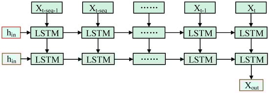
Figure 5.
Data processing including LSTM networks.
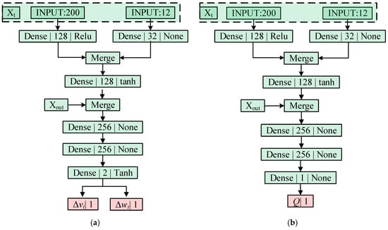
Figure 6.
The neural network structure designed in this paper. (a) shows the Actor neural network structure; (b) shows the Critic neural network structure.
Linear and angular velocities using Actor policy outputs to direct control of the robot will result in violent vibrations, so here, the robot velocity is controlled using an incremental approach. Assuming that the outputs of Actor are and , the velocity of the robot’s motion at the current moment is , the maximum acceleration and angular acceleration allowed for the robot are and , respectively, and since the output range of the activation function tanh is , the amount of the velocity of the control robot is and , respectively. Considering the structure of the robot, the driving force of the motors, and the smoothness of the motion, a dynamic window is usually used to constrain the control speed of the robot, assuming that the minimum and maximum permissible speeds of the robot are and , respectively, and the minimum and maximum permissible angular velocities are and , respectively, and the control speed of the robot at the next moment satisfies Equation (23).
5. Experimental Results
In this paper, during the simulation experiments, the learning rate is set to 0.001 when the SAC algorithm is used alone, and after the introduction of LSTM, the learning rate of the algorithm is set to 0.0001. During the actual experiments, the learning rate of the SAC_LSTM algorithm proposed in this paper is set to 0.001. The PPO and DDPG algorithms [,] have a similar structure to the SAC algorithm and have the same algorithmic learning rate settings. The activation functions involved in the above three algorithms mainly include ReLU [] and Tanh [].
5.1. Simulation Experiment Results
In this section, we conduct experiments on SAC-based reinforcement-learning navigation policy and analyze the performance in terms of different reinforcement-learning methods, the introduction of imitation learning with prioritized replay techniques, and the introduction of Recurrent Neural Networks. The computer configuration for the experiment was Intel I7 7700K CPU, the graphics card was NVIDIA 1060, and the operating system was Ubuntu 18.04. The deep learning framework used was TensorFlow 1.14 developed by Google Inc. (Mountain View City, CA, USA).
5.1.1. Performance Comparison of Reinforcement-Learning Navigation Policies
As shown in Figure 7, the simulation environment is built in Gazebo, and the size of the simulation environment is approximate to the size of the real environment in the laboratory, with a length and width of about 32 m and 16 m, respectively, and the maximum measurement depth of the robot-configured LiDAR is 20 m. The navigation target points for the test are randomly selected positions and directions in the six green areas in the figure, with position centers at , , , , , and , respectively, and the position coordinates are in meters with a radius of . Path navigation is considered successful when the positional distance between the robot and the target point is less than and the angular deviation is less than .
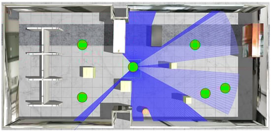
Figure 7.
Constructed simulation environment.
Trained in the same simulation environment, the cumulative reward values for each episode based on DDPG, PPO and the SAC reinforcement-learning navigation policy proposed in this paper is shown in Figure 8a, and the navigation success rate of the training process is shown in Figure 8b. The total number of training episodes and their distribution during the training process are shown in Figure 9.
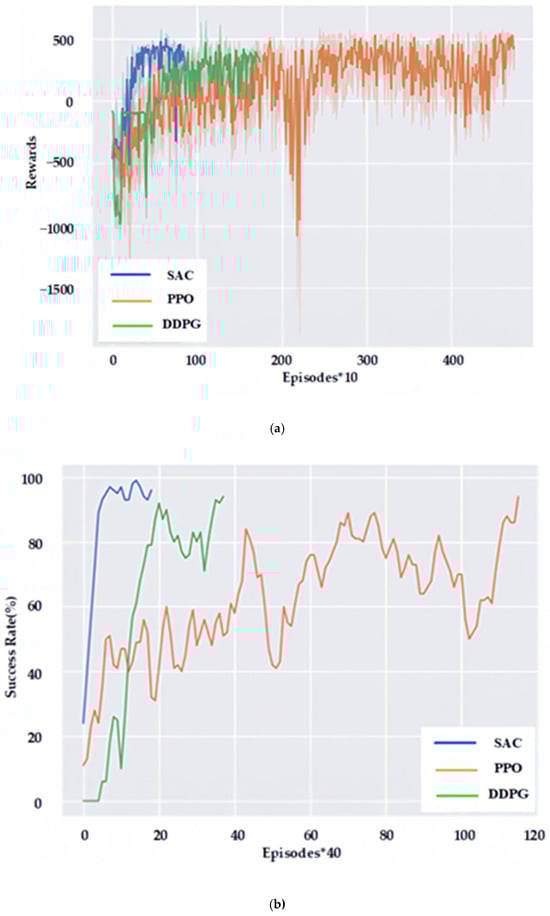
Figure 8.
Comparison of training reward values and success rates for reinforcement-learning methods. (a) is the result of reward value comparison; (b) is the result of success rate comparison.
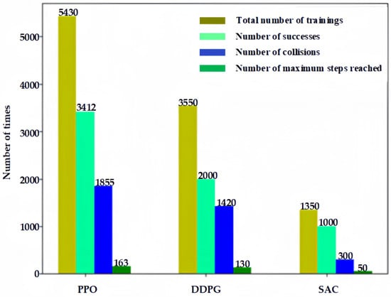
Figure 9.
Comparison of training times and performance.
As can be seen from Figure 8, the offline reinforcement-learning navigation policy of SAC proposed in this paper is the most effective, which only needs 887 episodes to achieve a 96% navigation success rate. The DDPG-based reinforcement-learning navigation policy is the second-most-effective, which can achieve a 94% navigation success rate in 1751 episodes, and the PPO-based reinforcement-learning navigation policy is less effective, which needs 4751 episodes to achieve a 94% navigation success rate, and the training time is close to 48 h.
As can be seen in Figure 9, the SAC reinforcement-learning method proposed in this paper can achieve a success rate of more than 94% with fewer episodes, and at the same time requires fewer collisions, which is safer for training and conducive to application in practical environments.
After the training is completed, the robot is allowed to run at the same starting position , with a yaw angle of , to the same six navigation target points, namely , , , , and . The yaw angle of the target point is . The distance between the robot and the target point is less than , and an angle deviation of less than is considered successful navigation. The number of steps run by the robot when the navigation is successful is recorded, and each target point is counted 100 times, and the results are shown in Figure 9.
It can be seen from Figure 10 that both the offline-based DDPG and the SAC proposed in this paper have better navigation effects on the six test points after the training is completed. However, the SAC in this paper has the best effect, which can reach the target point with fewer steps and can go through a shorter path to reach the target point with the best effect. Compared to the first two methods, the online-based PPO reinforcement-learning method, which requires more steps to reach the target point, has the worst navigation effect. For example, on the first target point, the average number of steps needed to reach the target point by the PPO-based reinforcement-learning method is 107.59, while the average number of steps needed to reach the target point by the DDPG-based and SAC-based reinforcement-learning methods proposed in this paper are only 40.52 and 32.78, respectively.
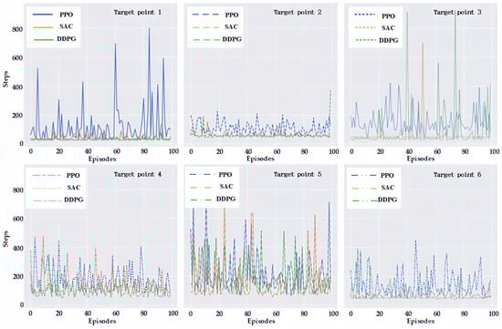
Figure 10.
Number of execution steps required to reach each target point.
5.1.2. Performance Comparison after Introduction of Imitation Learning and Improved Experience Replay Techniques
This section focuses on the analysis of the performance of SAC reinforcement-learning navigation policies using different prioritized experience replay techniques, including the Q-value-based replay technique and the prioritized experience replay technique proposed in this paper. The training reward values and success rates with or without using the prioritized replay technique and with different prioritized replay techniques are shown in Figure 10.
As can be seen in Figure 11, due to the difference between the data collected by the agent method and the expert data, the reward value and the success rate fluctuate during the training process. However, based on the prioritized experience replay technique proposed in this paper, the agent can achieve a high success rate in the initial stage, because the robot can “extricate” itself and quickly reach the target point, which greatly reduces the number of collisions between the robot and the environment, thus improving the training speed of the agent.
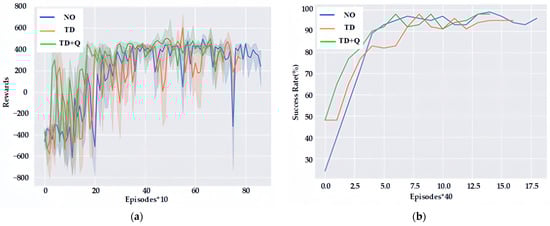
Figure 11.
Training reward values and success rates for different experience replay methods. (a) is the result of reward value comparison; (b) is the result of success rate comparison.
As can be seen in Figure 12, when no expert data are introduced (NO), 887 episodes are needed to achieve a 96% navigation success rate, and 772 episodes are needed to achieve a 95% navigation success rate by introducing imitation learning and a time-differential error (TD)-based replay technique. However, in this paper, the introduction of imitation learning and improved prioritization of the experience replay technique (TD+Q) can achieve a 98% success rate with only 701 episodes. What is more, the number of robot collisions can be further reduced from 305 to 224 and 113, respectively, after the introduction of imitation learning, thus making the training safer.
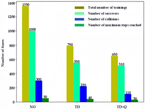
Figure 12.
Comparison of training times and performance.
5.1.3. Comparison of Dynamic Obstacle Avoidance with the Introduction of RNN
In order to verify the dynamic obstacle-avoidance ability of the planner after the introduction of Recurrent Neural Network, dynamic objects are added into the simulation environment for testing, as shown in Figure 13. Dynamic objects move within the circumference of the circle, and when they reach the boundary of the circle, the other side of the diameter is selected as the new target point, and the dynamic objects can sense each other’s position and velocity and perform obstacle-avoidance movement using the RVO algorithm [].
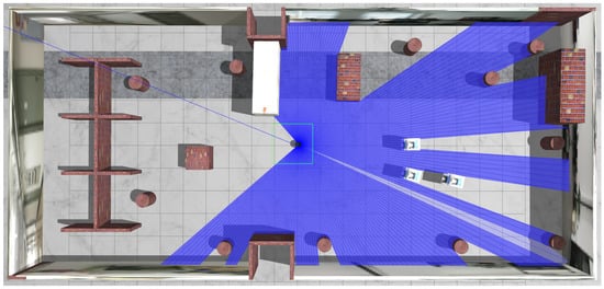
Figure 13.
Adding dynamic objects to the simulation environment.
The change process of the reward value and success rate of the training process in the dynamic environment is shown in Figure 14, which shows that after the introduction of the LSTM network, it can achieve a higher navigation success rate of more than 90% in a shorter period of time. However, when Recurrent Neural Networks are not used, obstacle avoidance is less effective because the inputs do not contain temporal information, their reward values are even lower, and the success rate is only about 80%. PPO_LSTM is a reinforcement-learning navigation strategy for solving the problem of obstacle avoidance for robots in dynamic environments, as proposed in the literature [].
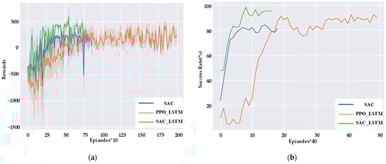
Figure 14.
Comparison of retraining reward values and success rates in a dynamic environment. (a) is the result of reward value comparison; (b) is the result of success rate comparison.
As can be seen in Figure 14, the PPO_LSTM method can also obtain a better navigation success rate after the introduction of Recurrent Neural Networks, but its training efficiency and navigation success rate are lower than the SAC_LSTM method proposed in this paper due to its use of an online approach to agent training and lack of stochastic exploration.
After training, the dynamic obstacle-avoidance process of the robot is shown in Figure 15. Figure 15 shows the movement of the robot from one planning point (initial point) to another planning point (target point), during which dynamic obstacle avoidance is constantly performed. In order to improve the agent’s reasoning ability, multiple static cylinders are added to the environment to make the laser measurements complex and closer to the real environment.
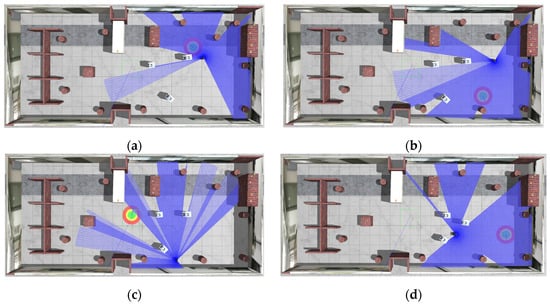
Figure 15.
Dynamic obstacle-avoidance process. (a–d) show the dynamic obstacle-avoidance process during the movement of the robot from one planning point (initial point) to another planning point (target point).
5.2. Practical Experimental Results
In order to verify the navigation performance of the SAC depth-enhanced navigation control method proposed in this paper in real applications, mobile robot navigation experiments are conducted in the indoor built environment in this section. Firstly, in order to verify the migration ability of the navigation policy, the trained agent in the simulation environment is utilized in the static environment and directly applied to the real environment for the navigation success rate test. The agent and the environment are interacted and trained again to improve the performance of the agent. Secondly, in order to verify the dynamic obstacle-avoidance performance of the navigation strategy, the dynamic obstacle-avoidance experiments are conducted in the dynamic obstacle environment for the agent after the interaction training is completed.
5.2.1. Testing and Policy Migration in Static Environments
For the robot navigation policy research objective of this paper, we need to apply the policy in the simulation environment to the real environment, i.e., policy migration. Utilizing the trained navigation policies in the simulation environment can greatly reduce the number of training samples needed in the real environment. An indoor navigation environment similar to the simulation environment was built in the laboratory, as shown in Figure 16a, and a map of the environment was constructed using LiDAR, as shown in Figure 16b. This environment map can provide localization information for the robot during navigation. The agent navigation planner obtained by training based on PPO, DDPG and the SAC reinforcement-learning algorithm proposed in this paper, respectively, is directly applied to the indoor environment for testing in the simulation environment.
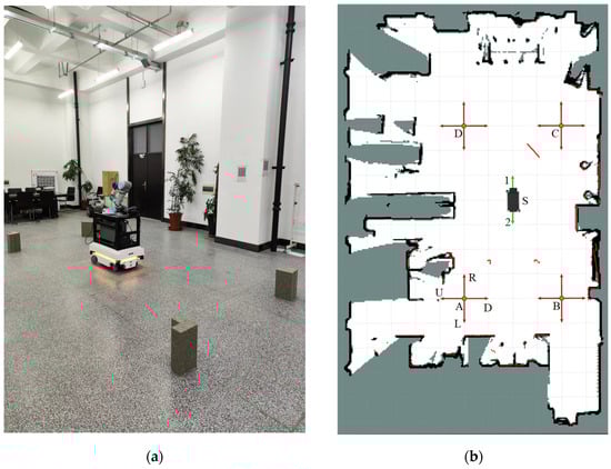
Figure 16.
Experimental scenarios and test target point settings. (a) is the test environment; (b) is the location of the planning point set in the environment map. In Figure 15b, S is the planned starting position with coordinates . Two test directions, 1 and 2, are considered, and the target points are located at A, B, C, and D with coordinates , , and , respectively, and the four directions of up (U), down (D), left (L), and right (R) are tested at each position.
The conditions for successful robot navigation are a distance range less than and an angle range less than ; this is based on the PPO, DDPG and SAC navigation strategy proposed in this paper, which succeeded 15, 19 and 23 times, respectively. The test results for planning points A, B, C and D are shown in Table 1. From Table 1, it can be seen that the performance of our navigation policy method is optimal, and its success rate can reach 71.9%, while the success rate of the other two methods can only reach about 45%.

Table 1.
Statistics on the results of target point navigation.
When the navigation policy is transferred to a real environment, the navigation success rates of the above methods are significantly reduced—a phenomenon known as the reality gap. In order to eliminate the reality gap phenomenon so that the navigation strategies can be applied to real environments, we allowed the robot to re-collect data in the physical environment for training. The change in navigation success rate during training is shown in Figure 17, and the final navigation success rate reaches 92%.
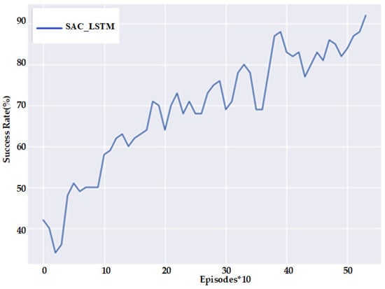
Figure 17.
Navigation success rate of this paper’s method during retraining in real scenarios.
After the training was completed, we had the robot perform a loop closure test, as shown in Figure 18. In Figure 18, the left side is the physical picture, and the bottom right side is the trajectory map displayed in RVIZ. The sequence of the robot’s running target points is S-1→A-D→B-R→C-U→D-L→S-2, which shows that the agent after training demonstrates a strong navigation and obstacle-avoidance ability and can move from an arbitrary position to another position without the need to set the starting position relatively fixedly. In order to verify the computational efficiency of the reinforcement-learning-based navigation policy, we counted 1300 times of the speed computation process, and its computational time consumed is shown in Figure 19.
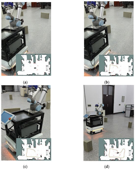
Figure 18.
Navigation planning process for loop closure motions. (a) is the robot at the starting position S-1; (b) is the robot arriving at the planning point position B-R; (c) is the robot arriving at the planning point position C-U; and (d) is the robot arriving at the end position S-2.
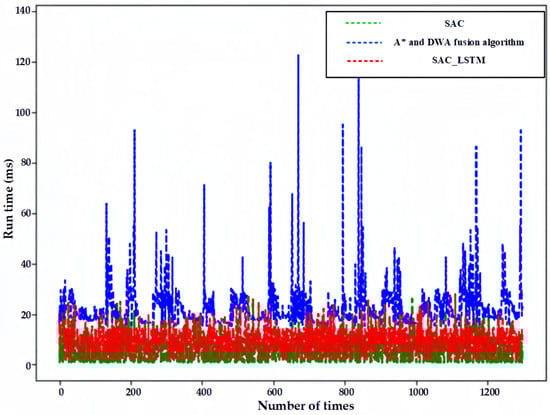
Figure 19.
Comparison of computation times for speed commands.
As can be seen in Figure 19, the average computation time of the fast path-generation algorithm (A* and DWA fusion algorithm) for calculating speed control commands is 23.527 ms, and the average computation time of the reinforcement-learning method without a Recurrent Neural Network (SAC) is 6.378 ms, and after the introduction of the Recurrent Neural Network (SAC_LSTM), the network parameters involved in computation are more, resulting in a slight increase in computation time to 9.557 ms. However, this is significantly lower than that of the traditional navigation algorithm, which is only 40.62%.
5.2.2. Obstacle-Avoidance Experiments in Dynamic Environments
In order to verify the effectiveness of the Recurrent Neural Network designed in this paper in dynamic environments, dynamic obstacle-avoidance experimental tests are conducted in indoor dynamic environments in this section. The successive processes of static obstacle avoidance and dynamic obstacle avoidance of the robot planner are displayed in RVIZ, as shown in Figure 20. The robot starts moving from the starting position, as shown in Figure 20a, and then senses static obstacles and performs obstacle avoidance, as shown in Figure 20b,c; then, after passing through static obstacles, the robot senses dynamic obstacles and generates an obstacle-avoidance trajectory, as shown in Figure 20d, after which the robot runs towards the planning target point, as shown in Figure 20e,f. The practical scenario of the robot bypassing static and dynamic obstacles is shown in Figure 21.
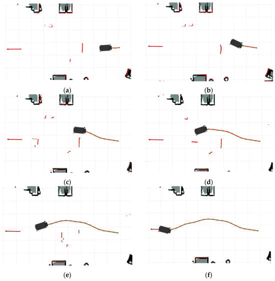
Figure 20.
Obstacle-avoidance process of the planner trained by the method of this paper. (a) shows the initial state of the robot; (b) shows the robot avoiding a static obstacle; (c) shows the robot passing through a static obstacle; (d) shows the robot avoiding dynamic obstacles; (e) shows the robot running towards the end point; and (f) shows the robot reaching the end point.
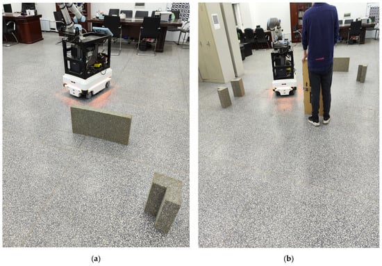
Figure 21.
Dynamic obstacle avoidance process for real scenarios. (a) shows the robot avoiding static obstacles (b) shows the robot avoiding dynamic obstacles.
The robot is allowed to plan continuously 20 times, and the statistical planning results are shown in Table 2.
Table 2.
Comparison of average running time and distance.
As can be seen from Table 2, we use the sequence information for stacking as the state information of the input Recurrent Neural Network, and the success rate of the obstacle avoidance of the robot navigation system in the dynamic scene is much higher than that of the ordinary fully connected neural network. Additionally, the average distance of operation is also smaller, but after the introduction of the neural network, the parameters become more parameters, which makes the computation time longer; however, the average distance is still much smaller than that of the traditional navigation and obstacle-avoidance methods. The main reasons for the reduced success rate of obstacle avoidance using this paper’s method in real environments are as follows: first, there is a difference between real and simulated environments, and second, the robot does not collect enough data in the real environment that can be used for the training of the agent.
6. Conclusions
In this paper, we propose a SAC reinforcement-learning navigation planner with an RNN. This solves the problem of low training efficiency caused by the uncertainty of the initial and hidden states of the RNN by adopting the sliding-window method to input the state data and realizes the efficient obstacle avoidance of the mobile robot in the environment of larger scenes and dynamic obstacles.
In future work, we will investigate how to quickly migrate trained models to practical environments. In addition, we will consider new network models and design new network structures and data preprocessing methods to generalize agents from small training environments to larger new environments. Meanwhile, less attention has been paid to the effect of dynamic obstacle movement speed on obstacle-avoidance methods, which we will investigate in depth.
Author Contributions
Project administration, Y.L.; writing—original draft preparation, C.W.; Data Curation, C.Z.; Formal analysis, H.W.; Supervision, Y.W. All authors have read and agreed to the published version of the manuscript.
Funding
This research was funded by Key Special Projects of Heilongjiang Province’s Key R&D Program (NO. 2023ZX01A01) and Heilongjiang Province’s Key R&D Program: ‘Leading the Charge with Open Competition’ (NO. 2023ZXJ01A02).
Data Availability Statement
The original contributions presented in the study are included in the article, further inquiries can be directed to the corresponding author.
Conflicts of Interest
The authors declare no conflicts of interest.
References
- Dai, Y.; Yang, S.; Lee, K. Sensing and Navigation for Multiple Mobile Robots Based on Deep Q-Network. Remote Sens. 2023, 15, 4757. [Google Scholar] [CrossRef]
- Xu, Y.H.; Wei, Y.R.; Jiang, K.Y.; Wang, D.; Deng, H.B. Multiple UAVs Path Planning Based on Deep Reinforcement Learning in Communication Denial Environment. Mathematics 2023, 11, 405. [Google Scholar] [CrossRef]
- Dayan, P.; Watkins, C. Q-learning. Mach. Learn. 1992, 8, 279–292. [Google Scholar] [CrossRef]
- Sutton, R.S. Generalization in reinforcement learning: Successful examples using sparse coarse coding. In Proceedings of the 9th Annual Conference on Neural Information Processing Systems (NIPS), Denver, Co, USA, 27–30 November 1995; pp. 1038–1044. [Google Scholar]
- Mnih, V.; Kavukcuoglu, K.; Silver, D.; Graves, A.; Antonoglou, I.; Wierstra, D.; Riedmiller, M. Playing atari with deep reinforcement learning. arXiv 2013, arXiv:1312.5602. [Google Scholar] [CrossRef]
- Van Hasselt, H.; Guez, A.; Silver, D. Deep reinforcement learning with double q-learning. In Proceedings of the AAAI Conference on Artificial Intelligence, Phoenix, AZ, USA, 12–17 February 2016; pp. 2094–2100. [Google Scholar]
- Wang, Z.; Schaul, T.; Hessel, M.; Hasselt, H.; Lanctot, M.; Freitas, N. Dueling network architectures for deep reinforcement learning. In Proceedings of the International conference on machine learning, New York, NY, USA, 20–22 June 2016; pp. 1995–2003. [Google Scholar]
- Schaul, T.; Quan, J.; Antonoglou, I.; Silver, D. Prioritized experience replay. arXiv 2015, arXiv:1511.05952. [Google Scholar] [CrossRef]
- Heess, N.; Tb, D.; Sriram, S.; Lemmon, J.; Merel, J.; Wayne, G.; Tassa, Y.; Erez, T.; Wang, Z.; Eslami, S. Emergence of locomotion behaviours in rich environments. arXiv 2017, arXiv:1707.02286. [Google Scholar] [CrossRef]
- Schulman, J.; Wolski, F.; Dhariwal, P.; Radford, A.; Klimov, O. Proximal policy optimization algorithms. arXiv 2017, arXiv:1707.06347. [Google Scholar] [CrossRef]
- Lillicrap, T.P.; Hunt, J.J.; Pritzel, A.; Heess, N.; Erez, T.; Tassa, Y.; Silver, D.; Wierstra, D. Continuous control with deep reinforcement learning. arXiv 2015, arXiv:1509.02971. [Google Scholar] [CrossRef]
- Silver, D.; Lever, G.; Heess, N.; Degris, T.; Wierstra, D.; Riedmiller, M. Deterministic policy gradient algorithms. In Proceedings of the International Conference on Machine Learning, Bejing, China, 22–24 June 2014; pp. 387–395. [Google Scholar]
- Haarnoja, T.; Tang, H.; Abbeel, P.; Levine, S. Reinforcement learning with deep energy-based policies. In Proceedings of the International conference on machine learning, Sydney, Australia, 6–11 August 2017; pp. 1352–1361. [Google Scholar]
- Haarnoja, T.; Zhou, A.; Hartikainen, K.; Tucker, G.; Ha, S.; Tan, J.; Kumar, V.; Zhu, H.; Gupta, A.; Abbeel, P. Soft actor-critic algorithms and applications. arXiv 2018, arXiv:1812.05905. [Google Scholar] [CrossRef]
- Tai, L.; Liu, M. A robot exploration strategy based on q-learning network. In Proceedings of the 2016 IEEE International Conference on Real-Time Computing and Robotics (rcar), Angkor Wat, Cambodia, 6–10 June 2016; pp. 57–62. [Google Scholar]
- Jaradat, M.A.K.; Al-Rousan, M.; Quadan, L.J.R.; Manufacturing, C.-I. Reinforcement based mobile robot navigation in dynamic environment. Robot. Comput.-Integr. Manuf. 2011, 27, 135–149. [Google Scholar] [CrossRef]
- Fang, Q.; Xu, X.; Wang, X.; Zeng, Y. Target-driven visual navigation in indoor scenes using reinforcement learning and imitation learning. CAAI Trans. Intell. Technol. 2022, 7, 167–176. [Google Scholar] [CrossRef]
- Yang, Q.; Simão, T.D.; Tindemans, S.H.; Spaan, M.T. WCSAC: Worst-case soft actor critic for safety-constrained reinforcement learning. In Proceedings of the AAAI Conference on Artificial Intelligence, Virtual, 2–9 February 2021; pp. 10639–10646. [Google Scholar]
- Dalal, G.; Dvijotham, K.; Vecerik, M.; Hester, T.; Paduraru, C.; Tassa, Y. Safe exploration in continuous action spaces. arXiv 2018, arXiv:1801.08757. [Google Scholar] [CrossRef]
- Stooke, A.; Achiam, J.; Abbeel, P. Responsive safety in reinforcement learning by pid lagrangian methods. In Proceedings of the International Conference on Machine Learning, Virtual, 13–18 July 2020; pp. 9133–9143. [Google Scholar]
- Liu, Y.; Wang, C.; Wu, H.; Wei, Y. Mobile Robot Path Planning Based on Kinematically Constrained A-Star Algorithm and DWA Fusion Algorithm. Mathematics 2023, 11, 4552. [Google Scholar] [CrossRef]
- Zhang, L.; Jia, X.L.; Tian, N.; Hong, C.S.; Han, Z. When Visible Light Communication Meets RIS: A Soft Actor-Critic Approach. IEEE Wirel. Commun. Lett. 2024, 13, 1208–1212. [Google Scholar] [CrossRef]
- Li, T.J.; Guan, Z.W.; Zou, S.F.; Xu, T.Y.; Liang, Y.B.; Lan, G.H. Faster algorithm and sharper analysis for constrained Markov decision process. Oper. Res. Lett. 2024, 54, 107107. [Google Scholar] [CrossRef]
- Chen, Y.; Shen, X.; Zhang, G.; Lu, Z. Multi-Objective Multi-Satellite Imaging Mission Planning Algorithm for Regional Mapping Based on Deep Reinforcement Learning. Remote Sens. 2023, 15, 3932. [Google Scholar] [CrossRef]
- Nair, V.; Hinton, G.E. Rectified linear units improve restricted boltzmann machines. In Proceedings of the 27th International Conference on Machine Learning (ICML-10), Haifa, Israel, 21–24 June 2010; pp. 807–814. [Google Scholar]
- Ghanimi, H.M.A.; Gopalakrishnan, T.; Deol, G.J.S. Chebyshev polynomial approximation in CNN for zero-knowledge encrypted data analysis. J. Discret. Math. Sci. Cryptogr. 2024, 27, 203–214. [Google Scholar] [CrossRef]
- Van Den Berg, J.; Guy, S.J.; Lin, M.; Manocha, D. Reciprocal n-body collision avoidance. In Proceedings of the Robotics Research: The 14th International Symposium ISRR, Lucerne, Switzerland, 31 August–3 September 2011; pp. 3–19. [Google Scholar]
- Liu, S.; Chang, P.; Liang, W.; Chakraborty, N.; Driggs-Campbell, K. Decentralized structural-rnn for robot crowd navigation with deep reinforcement learning. In Proceedings of the 2021 IEEE International Conference on Robotics and Automation (ICRA), Xian, China, 30 May–5 June 2021; pp. 3517–3524. [Google Scholar]
Disclaimer/Publisher’s Note: The statements, opinions and data contained in all publications are solely those of the individual author(s) and contributor(s) and not of MDPI and/or the editor(s). MDPI and/or the editor(s) disclaim responsibility for any injury to people or property resulting from any ideas, methods, instructions or products referred to in the content. |
© 2024 by the authors. Licensee MDPI, Basel, Switzerland. This article is an open access article distributed under the terms and conditions of the Creative Commons Attribution (CC BY) license (https://creativecommons.org/licenses/by/4.0/).