Characteristics of Cloud and Aerosol Derived from Lidar Observations during Winter in Lhasa, Tibetan Plateau

Abstract

In order to investigate the variations of cloud and aerosol vertical profiles over the Tibetan Plateau (TP) in winter, we performed ground-based lidar observations in Lhasa, a city on the TP, from November 2021 to January 2022. The profiles of extinction coefficient, depolarization ratio, and signal-to-noise ratio (SNR) were retrieved using the atmospheric echo signals collected by the lidar. Clouds were identified by the range-correction echo signals and classified into water clouds, mixed clouds, horizontally oriented ice crystal clouds (HOICC), and ice clouds by the depolarization ratio and the hourly temperature from the European Centre for Medium-Range Weather Forecasts Reanalysis version 5 (ERA5). The clouds mainly appeared at a height of 3~5 km from 14:00–22:00 Beijing Time throughout the field campaign. The height and frequency (~30%) for cloud appearance were significantly lower than that reported in previous studies in summer. The cloud categories were dominated by mixed clouds and ice clouds during the observation period. The proportions of ice clouds gradually increased with increasing heights. After eliminating profiles influenced by clouds, the aerosol extinction coefficient and depolarization ratio were obtained, and the atmospheric boundary layer height (ABLH) was calculated. The aerosol extinction coefficient decreased with increasing height in the ABLH, and there were no obvious changes for the aerosol extinction coefficient above the ABL. The aerosol extinction coefficients near the Earth’s surface presented two peaks, appearing in the morning and evening, respectively. The high aerosols at the surface in the morning continually spread upward for 4–5 h and finally reached an altitude of 1 km with the development of ABLH. In addition, the depolarization ratio of aerosols decreased slowly with increasing altitudes. There was no obvious diurnal variation for depolarization ratios, indicating partly that the source of aerosols did not change significantly. These results are beneficial in understanding the evolution of cloud and aerosol vertical profiles over the TP.

1. Introduction

Clouds and aerosols are important for many physical and chemical processes in the atmosphere. Clouds determine the surface precipitation and atmospheric radiation balance [1,2]. Aerosol particles can be used as cloud condensation nuclei to change the microphysical properties of clouds and then affect the radiative forcing of clouds. They also affect the energy balance of the Earth-atmosphere system by scattering and absorbing short-wave solar radiation and emitting and capturing long-wave radiation [3,4,5]. Tibetan Plateau (TP) is located in the central and eastern parts of the Eurasian continent and serves as a role of ‘‘the world water tower’’ [6]. Due to its unique landform, fragile ecosystem, and particular monsoon circulation, TP is considered a sensitive area for human activities [7]. The dust aerosol over the TP can heat the middle troposphere by absorbing solar radiation. The heating produces atmospheric dynamical feedback, i.e., the so-called elevated-heat-pump (EHP) effect, which enhances the rate of snow melt in the Himalayas and TP [8]. The increase of cloud cover on the lee slope of the TP increases the surface temperature, which leads to the destabilization and desaturation in the boundary layer [9]. In addition, the increase of low-level cloud cover at night is greater than the decrease of low-level cloud cover and total cloud cover in daytime, which influences surface temperature and its range of diurnal variation over the TP [10]. Investigating the spatiotemporal variations of cloud and aerosol on the TP can help us to understand the effects of their radiative feedback on the climate and environment in this region.

Lhasa is one of the major cities on the TP, with an average elevation of more than 3600 m [11]. Due to urbanization and tourism development, fossil fuels have become the primary energy consumption in Lhasa [12]. Primitive biomass burning and religious burning also occur frequently [13]. There have been some studies focusing on the variation characteristics of clouds and aerosols over the TP. It was shown that the cloud cover in July over the TP accounted for a high proportion throughout the day due to the influence of monsoons, especially in the southern and northwestward areas of the TP, and the semidiurnal (2:00–10:00 UTC) cloud-cover cycle was weaker in July than in January, April, and October [14]. The dependences of cloud cover on altitude over the TP were found to show an obvious seasonal variation, with a single peak (7~11 km) from January to April, double peaks (5~8 km and 11~17 km, respectively) after mid-June, and a single peak (5~10 km) after mid-August [15]. According to the CALIPSO (Cloud-Aerosol Lidar and Infrared Pathfinder Satellite Observation) aerosol observation, the dust plume in spring over the TP is mainly from the desert and the Gobi region in the northeastern TP [16]. In addition, the local religious burning in Lhasa in summer is a significant potential source of aerosols and accounts for 80% of total source emissions on the religious activity days [13]. However, the vertical distribution of clouds and aerosols over the TP in winter are still not fully understood at present.

In recent years, lidar has been widely used for remote sensing detection of clouds and aerosols [17]. Lidar has the advantages of high spatial and temporal resolution in obtaining profile information of atmospheric features. Based on polarization detection technology, the parallel and perpendicular polarization components of the received backscattered signal are separated and then the corresponding depolarization ratios are calculated [18]. The depolarization ratio is used to distinguish the scattering of spherical particles from non-spherical particles and identify aerosols, cloud droplets, and ice crystals [18,19,20]. The joint observations of lidar and weather radar in summer in Naqu, Tibet indicated that the frequency of low clouds in summer is about 50%, the frequency of liquid clouds and mixed phase clouds is higher in the morning and afternoon, and ice clouds mainly occur in the afternoon and midnight [2]. The polarization lidar observations in Litang and Naqu over the TP showed that the average depolarization ratio is 0.44 for cirrus clouds, and the height of cirrus clouds is between 5.2–12 km above ground level. The depolarization ratio of cirrus particles increases with increasing height, but the situation for the particle depolarization ratio is opposite [21]. The observations by satellite-borne lidar CALIOP (Cloud-Aerosol Lidar with Orthogonal Polarization) from 2007 to 2014 found that the dust on the TP mainly came from the Taklimakan Desert, in addition to the Gurbantunggut Desert and the Great Indian Thar Desert in some cases [22]. These studies have mainly concentrated on the characteristics of clouds and aerosol in summer over the TP through lidar observations. The lidar observations of clouds and aerosols over the TP are scarce in winter, and their spatiotemporal evolutions are not yet fully understood.

In this study, we performed ground-based lidar observations in Lhasa from 2 November 2021 to 25 January 2022. Clouds were identified by the range-corrected lidar signal and classified by the depolarization ratios and hourly temperature profiles from ERA5. The vertical distributions and diurnal variations of the extinction coefficient and depolarization ratio were also investigated. Section 2 introduces the observation site and instrument, as well as the methods for the extinction coefficient and depolarization ratio retrieval, cloud identification, and classification. Section 3 presents the vertical distribution and its temporal evolution of cloud, extinction coefficient, and depolarization ratio during the observation period. Finally, a discussion and conclusions are provided in Section 4 and Section 5, respectively.

2. Materials and Methods

2.1. Site and Instrument

The lidar observations were performed at the Lhasa Meteorological Station (91.14°E, 29.66°N, altitude 3552.5 m, a.s.l) in the downtown of Lhasa, the capital of the Tibet Autonomous Region, from 2 November 2021 to 25 January 2022. Within a radius of 3 km around the site, there are mainly low buildings, including several temples (such as Jokhang Temple and Norbulingka Temple), where spices and biomass fuels are burned for religious activities. In addition, the world-famous Potala Palace is located about 1.5 km southwest of the site. The site belongs to the temperate monsoon semi-arid plateau climate, characterized by strong solar radiation, long sunny days, low rainfall, and cold and dry winters. The Barkhor Street ambient air quality monitoring station is about 500 m away, southwest of the site, where hourly concentrations of surface particulate matter 2.5 (PM_2.5) are operationally released in real time. More details of the natural and human environment around the observation site can be found in previous studies [12,23,24].

The lidar system used in the study was developed by the Anhui Institute of Optics and Fine Mechanics, Chinese Academy of Sciences (AIOFM, CAS). The lidar consists of a laser emitting system, a receiving system, a data acquisition system, and a control system [25]. The laser emitting system consists of a laser and an optical unit, which emits laser pulses at a wavelength of 532 nm into the atmosphere. The receiving system consists of a telescope and a subsequent optical system. The telescope belongs to a Cassegrain telescope with a field of view angle of less than 1 mrad and a diameter of 150 mm. The atmospheric backscattered light received by the telescope is split by the polarizing prism, filtered on each channel, and then detected by photomultiplier tubes (PMT). The echo signals can be obtained via the data acquisition system. The main technical specifications of the lidar system are given in

Table 1. Main technical specifications of lidar system.

Technical Parameters	Value
Lase type	Active Q-switched laser
Laser wavelength	532.09 nm
Pulse energy	0.154 mJ
Pulse repetition rate	4 kHz
Pulse width (FWHM)	5.945 ns
Laser beam divergence	x = 0.323 mrad, y = 0.329 mrad
Telescope type	Cassegrain
Telescope diameter	150 mm
Vertical resolution	7.5 m
Time resolution	1 s–1800 s, adjustable
Effective detection range	10 km
Lidar configuration type	biaxial
Overlap range	≈200 m

.

During the 85-day observation period, the lidar operated stably except for maintenance and power outages, and the data acquisition rate was approximately 95%. The original vertical resolution of the lidar was set to 7.5 m, with a temporal resolution of 5 min. During data pre-processing, the original signals were smoothed using a 7-point window, and the background noises were removed. In addition, data quality control was carried out based on the principle of 3 times standard deviation.

2.2. Retrieval of Extinction Coefficient and Depolarization Ratio

With the assumption of only single scattering, the lidar equation can be expressed as the following [26]:

$$\mathrm{P}\left(\mathrm{z},\mathrm{\lambda }\right)=\frac{\mathrm{C}}{{\mathrm{z}}^2}{\mathrm{P}}_0\left(\mathrm{\lambda }\right)\mathrm{\beta }\left(\mathrm{z},\mathrm{\lambda }\right)\exp \left(-2{\displaystyle {\int }_0^{\mathrm{z}}\mathrm{\alpha }\left(\mathrm{z},\mathrm{\lambda }\right)\mathrm{d}{\mathrm{z}}^{\prime }}\right),$$

(1)

where $\mathrm{P}\left(\mathrm{z},\mathrm{\lambda }\right)$ is the power of the echo signal at distance $\mathrm{z}$; $\mathrm{C}$ is the lidar system constant; ${\mathrm{P}}_0\left(\mathrm{\lambda }\right)$ is the initial laser emission power. The atmospheric backscatter coefficient $\mathrm{\beta }\left(\mathrm{z},\mathrm{\lambda }\right)$ is the sum of the atmospheric molecule backscatter coefficient ${\mathsf{\beta }}_{\mathrm{m}}\left(\mathrm{z},\mathsf{\lambda }\right)$ and the aerosol backscatter coefficient ${\mathsf{\beta }}_{\mathrm{a}}\left(\mathrm{z},\mathsf{\lambda }\right)$. The atmospheric extinction coefficient $\mathrm{\alpha }\left(\mathrm{z},\mathrm{\lambda }\right)$ is the sum of the atmospheric molecule extinction coefficient ${\mathrm{\alpha }}_{\mathrm{m}}\left(\mathrm{z},\mathrm{\lambda }\right)$ and the aerosol extinction coefficient ${\mathrm{\alpha }}_{\mathrm{a}}\left(\mathrm{z},\mathrm{\lambda }\right)$.

The aerosol extinction coefficients can be retrieved by the Collis method [27], the Klett method [28], and the Fernald method [29]; wherein the Fernald method is widely used with high inversion accuracy. In this study, we used the Fernald method to retrieve the extinction coefficient of aerosol. The Fernald method assumes that the backscattering coefficient of particles is proportional to the extinction coefficient, as shown in Equations (2) and (3):

$${\mathrm{S}}_{\mathrm{a}}=\frac{{\mathrm{\alpha }}_{\mathrm{a}}}{{\mathrm{\beta }}_{\mathrm{a}}}$$

(2)

$${\mathrm{S}}_{\mathrm{m}}=\frac{{\mathrm{\alpha }}_{\mathrm{m}}}{{\mathrm{\beta }}_{\mathrm{m}}}$$

(3)

Therefore, the aerosol backscatter coefficient can be written as follows [29]:

$${\mathrm{\beta }}_{\mathrm{a}}\left(\mathrm{z}\right)=-{\mathrm{\beta }}_{\mathrm{m}}\left(\mathrm{z}\right)+\frac{\mathrm{P}\left(\mathrm{z}\right){\mathrm{z}}^2\exp \left[2\left({\mathrm{S}}_{\mathrm{a}}-{\mathrm{S}}_{\mathrm{m}}\right){\displaystyle {\int }_{\mathrm{z}}^{{\mathrm{z}}_{\mathrm{c}}}{\mathrm{\beta }}_{\mathrm{m}}\left({\mathrm{z}}^{\prime }\right)\mathrm{d}{\mathrm{z}}^{\prime }}\right]}{\frac{\mathrm{P}\left({\mathrm{z}}_{\mathrm{c}}\right){{\mathrm{z}}_{\mathrm{c}}}^2}{{\mathrm{\beta }}_{\mathrm{a}}\left({\mathrm{z}}_{\mathrm{c}}\right)+{\mathrm{\beta }}_{\mathrm{m}}\left({\mathrm{z}}_{\mathrm{c}}\right)}+2{\displaystyle {\int }_{\mathrm{z}}^{{\mathrm{z}}_{\mathrm{c}}}{\mathrm{S}}_{\mathrm{a}}\mathrm{P}\left({\mathrm{z}}^{\prime }\right){{\mathrm{z}}^{\prime }}^2\exp \left[2\left({\mathrm{S}}_{\mathrm{a}}-{\mathrm{S}}_{\mathrm{m}}\right){\displaystyle {\int }_{\mathrm{z}}^{{\mathrm{z}}_{\mathrm{c}}}{\mathrm{\beta }}_{\mathrm{m}}\left({\mathrm{z}}^{″}\right)\mathrm{d}{\mathrm{z}}^{″}}\right]\mathrm{d}{\mathrm{z}}^{\prime }}}$$

(4)

where ${\mathrm{z}}_{\mathrm{c}}$ is the height of reference point, and ${\mathrm{S}}_{\mathrm{a}}$ is the ratio of extinction coefficient and backscatter coefficient for atmospheric aerosol (usually referred to as the lidar ratio). The lidar ratio is one of the important parameters for the retrieval of the aerosol extinction coefficient, which is related to the physical and chemical properties of the aerosol, such as composition, particle size distribution, and shape [30,31]. ${\mathrm{S}}_{\mathrm{m}}=8\mathrm{\pi }/3$ is the ratio of extinction coefficient and backscatter coefficient for atmospheric molecules. ${\mathsf{\beta }}_{\mathrm{m}}$ is calculated from the vertical profile of air molecule density provided by the American standard atmospheric model according to the Rayleigh scattering theory [32], where ${\mathrm{z}}_{\mathrm{c}}$ is the height of the reference point. ${\mathrm{\beta }}_{\mathrm{a}}\left({\mathrm{z}}_{\mathrm{c}}\right)$ at wavelength 532 nm is calculated by Equation (5) [33,34]:

$$1+\frac{{\mathrm{\beta }}_{\mathrm{a}}\left({\mathrm{z}}_{\mathrm{c}}\right)}{{\mathrm{\beta }}_{\mathrm{m}}\left({\mathrm{z}}_{\mathrm{c}}\right)}=1.01$$

(5)

The depolarization ratio is defined as the ratio of the cross-polarized signal to the parallelly polarized signal at the same wavelength, which is usually used as the indicator of particle shape. Commonly, a larger depolarization ratio corresponds to a more irregular shape of the particles [35]. In this study, the depolarization ratio was calculated by the 532 nm echo signal, as shown in Equation (6):

$$\mathrm{\delta }\left(\mathrm{z}\right)=\frac{{\mathrm{\beta }}_{532\perp }\left(\mathrm{z}\right)}{{\mathrm{\beta }}_{532\parallel }\left(\mathrm{z}\right)}$$

(6)

where $\mathrm{\delta }\left(\mathrm{z}\right)$ is the depolarization ratio; ${\mathrm{\beta }}_{532\perp }\left(\mathrm{z}\right)$ and ${\mathrm{\beta }}_{532\parallel }\left(\mathrm{z}\right)$ are the backscatter coefficients at the wavelength of 532 nm for cross and parallel polarization channels, respectively. Figure A1 shows the range-corrected echo signal, extinction coefficient and depolarization ratio profile on 10 November 2021, respectively.

2.3. Cloud Identification and Classification

Based on the range-corrected lidar signal, we use the method of value distribution equalization (VDE) to identify clouds [36]. The VDE method has several advantages, such as preventing the expansion of noises at far distances, making aerosol/cloud signals stand out clearly from noises, and making SNR at a far distance comparable to that at a near distance [36].

In the first part, the semi-discretization method (SDP) is used to reduce the influence of noise on the power of the echo signal $\mathrm{P}$ [37]. The background noise (signals at 14–15 km height above the surface in this study) is subtracted from $\mathrm{P}$ and the standard deviation (${\mathrm{\sigma }}_{\mathrm{n}}$) of the background noise is calculated. Then smoothing P with a window of 0.06 km obtains the processed echo signal ${\mathrm{P}}_{\mathrm{s}}\left(\mathrm{z}\right)$. The processing of ${\mathrm{P}}_{\mathrm{s}}\left({\mathrm{z}}_{\mathrm{i}}\right)\left(\mathrm{i}=1,2,3,\dots ,\mathrm{N}\right)$ is shown in Equations (7)–(9):

$${\mathrm{P}}_{\mathrm{d}1}\left(\mathrm{z}\right)=\{\begin{array}{c}{\mathrm{P}}_{\mathrm{s}}\left({\mathrm{z}}_{\mathrm{i}-1}\right),\left|{\mathrm{P}}_{\mathrm{s}}\left({\mathrm{z}}_{\mathrm{i}}\right)-{\mathrm{P}}_{\mathrm{s}}\left({\mathrm{z}}_{\mathrm{i}-1}\right)\right|<3{\mathrm{\sigma }}_{\mathrm{n}}\\ {\mathrm{P}}_{\mathrm{s}}\left({\mathrm{z}}_{\mathrm{i}}\right),\left|{\mathrm{P}}_{\mathrm{s}}\left({\mathrm{z}}_{\mathrm{i}}\right)-{\mathrm{P}}_{\mathrm{s}}\left({\mathrm{z}}_{\mathrm{i}-1}\right)\right|\ge 3{\mathrm{\sigma }}_{\mathrm{n}}\end{array},$$

(7)

$${\mathrm{P}}_{\mathrm{d}2}\left(\mathrm{z}\right)=\{\begin{array}{c}{\mathrm{P}}_{\mathrm{s}}\left({\mathrm{z}}_{\mathrm{i}+1}\right),\left|{\mathrm{P}}_{\mathrm{s}}\left({\mathrm{z}}_{\mathrm{i}}\right)-{\mathrm{P}}_{\mathrm{s}}\left({\mathrm{z}}_{\mathrm{i}+1}\right)\right|<3{\mathrm{\sigma }}_{\mathrm{n}}\\ {\mathrm{P}}_{\mathrm{s}}\left({\mathrm{z}}_{\mathrm{i}}\right),\left|{\mathrm{P}}_{\mathrm{s}}\left({\mathrm{z}}_{\mathrm{i}}\right)-{\mathrm{P}}_{\mathrm{s}}\left({\mathrm{z}}_{\mathrm{i}+1}\right)\right|\ge 3{\mathrm{\sigma }}_{\mathrm{n}}\end{array},$$

(8)

$${\mathrm{P}}_{\mathrm{d}}\left(\mathrm{z}\right)=\frac{{\mathrm{P}}_{\mathrm{d}1}\left(\mathrm{z}\right)+{\mathrm{P}}_{\mathrm{d}2}\left(\mathrm{z}\right)}{2},$$

(9)

where ${\mathrm{P}}_{\mathrm{d}}\left(\mathrm{z}\right)$ denotes the average of ${\mathrm{P}}_{\mathrm{d}1}\left(\mathrm{z}\right)$ and ${\mathrm{P}}_{\mathrm{d}2}\left(\mathrm{z}\right)$, which retains the characteristics of sharp signals and minimizes the impact of atmospheric turbulence.

The second part is to treat ${\mathrm{P}}_{\mathrm{d}}\left(\mathrm{z}\right)$ using the VDE method to identify clouds and aerosol layers. First, ${\mathrm{P}}_{\mathrm{d}}\left(\mathrm{z}\right)$ is sorted in ascending order to obtain the intermediate variable $\mathrm{R}\left(\mathrm{i}\right),\left(\mathrm{i}=1,2,3,\dots ,\mathrm{N}\right)$. The index of an element of $\mathrm{R}\left(\mathrm{i}\right)$ in ${\mathrm{P}}_{\mathrm{d}}\left(\mathrm{z}\right)$ is denoted as $\mathrm{I}\left(\mathrm{i}\right),\left(\mathrm{i}=1,2,3,\dots ,\mathrm{N}\right)$. The minimum and maximum values of ${\mathrm{P}}_{\mathrm{d}}\left(\mathrm{z}\right)$ are expressed as ${\mathrm{M}}_{\mathrm{I}}$ and ${\mathrm{M}}_{\mathrm{A}}$, respectively. Then, the scale mapping coefficients ${\mathrm{P}}_{\mathrm{e}}\left(\mathrm{i}\right)$ are shown as follows:

$${\mathrm{P}}_{\mathrm{e}}\left(\mathrm{i}\right)=\mathrm{i}/\mathrm{N},\left(\mathrm{i}=1,2,3,\dots ,\mathrm{N}\right),$$

(10)

$${\mathrm{P}}_{\mathrm{e}}\left(\mathrm{i}\right)=\{\begin{array}{c}{\mathrm{P}}_{\mathrm{e}}\left(\mathrm{i}-1\right),\mathrm{R}\left(\mathrm{i}\right)=\mathrm{R}\left(\mathrm{i}-1\right)\\ {\mathrm{P}}_{\mathrm{e}}\left(\mathrm{i}\right),\mathrm{R}\left(\mathrm{i}\right)=\mathrm{R}\left(\mathrm{i}\right)\end{array},$$

(11)

with ${\mathrm{P}}_{\mathrm{e}}\left(\mathrm{i}\right)$ and the signal ranges, new ascending data values can be calculated:

$$\mathrm{Y}\left(\mathrm{i}\right)={\mathrm{P}}_{\mathrm{e}}\left(\mathrm{i}\right)\left({\mathrm{M}}_{\mathrm{A}}-{\mathrm{M}}_{\mathrm{I}}\right)+{\mathrm{M}}_{\mathrm{I}},$$

(12)

Finally, a new dataset ${\mathrm{P}}_{\mathrm{N}}\left(\mathrm{z}\right)$ can be constructed via the aforementioned steps:

$${\mathrm{P}}_{\mathrm{N}}\left(\mathrm{z}\right)={\mathrm{P}}_{\mathrm{N}}\left[\mathrm{I}\left(\mathrm{i}\right)\right]=\mathrm{Y}\left(\mathrm{i}\right)$$

(13)

The baseline $\mathrm{B}\left(\mathrm{z}\right)$ is constructed from points $\left({\mathrm{z}}_1,{\mathrm{M}}_{\mathrm{A}}\right)$ and $\left({\mathrm{z}}_{\mathrm{N}},{\mathrm{M}}_{\mathrm{I}}\right)$. The position where ${\mathrm{P}}_{\mathrm{N}}\left(\mathrm{z}\right)$ is greater than $\mathrm{B}\left(\mathrm{z}\right)$ is regarded as the appearance of the cloud and aerosol layer. We removed layers with a thickness of less than 50 m, probably caused by random fluctuations [36].

The third part distinguishes the cloud layer from the aerosol layer by calculating the slope of the rising part and the falling part of the aforementioned identification layer. The following threshold function $\mathrm{F}\left(\mathrm{z}\right)$ should be constructed:

$$\mathrm{F}\left(\mathrm{z}\right)=\frac{\mathrm{dln}\left[\left({\mathrm{P}}_{\mathrm{b}}\left(\mathrm{z}\right){\mathrm{z}}^2\right)\right]}{\mathrm{d}\mathrm{z}},$$

(14)

where ${\mathrm{P}}_{\mathrm{b}}\left(\mathrm{z}\right)$ is the echo signal after subtracting the background noise. The maximum and minimum values of $\mathrm{F}\left(\mathrm{z}\right)$ are denoted as $\mathrm{K}$ and $\mathrm{D}$, respectively. The aerosol layer and cloud layer can be distinguished by Equation (15) [36,38,39]:

$$\mathrm{L}\mathrm{a}\mathrm{y}\mathrm{e}\mathrm{r}=\{\begin{array}{l}\mathrm{c}\mathrm{l}\mathrm{o}\mathrm{u}\mathrm{d},\mathrm{z}\le 3\mathrm{k}\mathrm{m},\mathrm{K}>3\mathrm{o}\mathrm{r}\mathrm{D}<-7\\ \mathrm{c}\mathrm{l}\mathrm{o}\mathrm{u}\mathrm{d},\mathrm{z}>3\mathrm{k}\mathrm{m},\mathrm{K}>1.5\mathrm{o}\mathrm{r}\mathrm{D}<-7\\ \mathrm{a}\mathrm{e}\mathrm{r}\mathrm{o}\mathrm{s}\mathrm{o}\mathrm{l}\end{array},$$

(15)

In addition to the clouds identified by the above method, the cloud phase can be further classified by using depolarization ratios and the ERA5 hourly temperature profile [40]. The temperature profile is gridded into 37 layers from 1000 hPa to 1 hPa and interpolated to match the temporal and vertical resolution of the lidar profile. According to the temperature and depolarization ratio data, the cloud phases are divided into four categories, i.e., water cloud, mixed phase cloud, horizontally oriented ice crystal cloud (HOICC), and ice cloud [2,41]. The classification basis is shown in

Table 2. Classification basis of cloud phase.

Cloud Phase	${\mathbf{\beta }}_{\mathbf{a}}(\mathbf{z})/({\mathbf{m}}^{-1}\mathbf{s}{\mathbf{r}}^{-1})$	T (°C)	$\mathbf{\delta }(\mathbf{z})$
water	>10−3	>0	$\mathrm{\delta }$ ≥ 0 and $\mathrm{\delta }$ ≤ 0.05
mixed	>10−3	≤0	$\mathrm{\delta }$ > 0.05 and $\mathrm{\delta }$ ≤ 0.3
HOICC	>10−3	<0	$\mathrm{\delta }$ ≥ 0 and $\mathrm{\delta }$ ≤ 0.05
ice	>10−3	<0	>0.3

where β_a(z) is the aerosol backscattering coefficient, T is the temperature by ERA5, and $\mathrm{\delta }(\mathrm{z})$ is the depolarization ratio.

:

3. Results

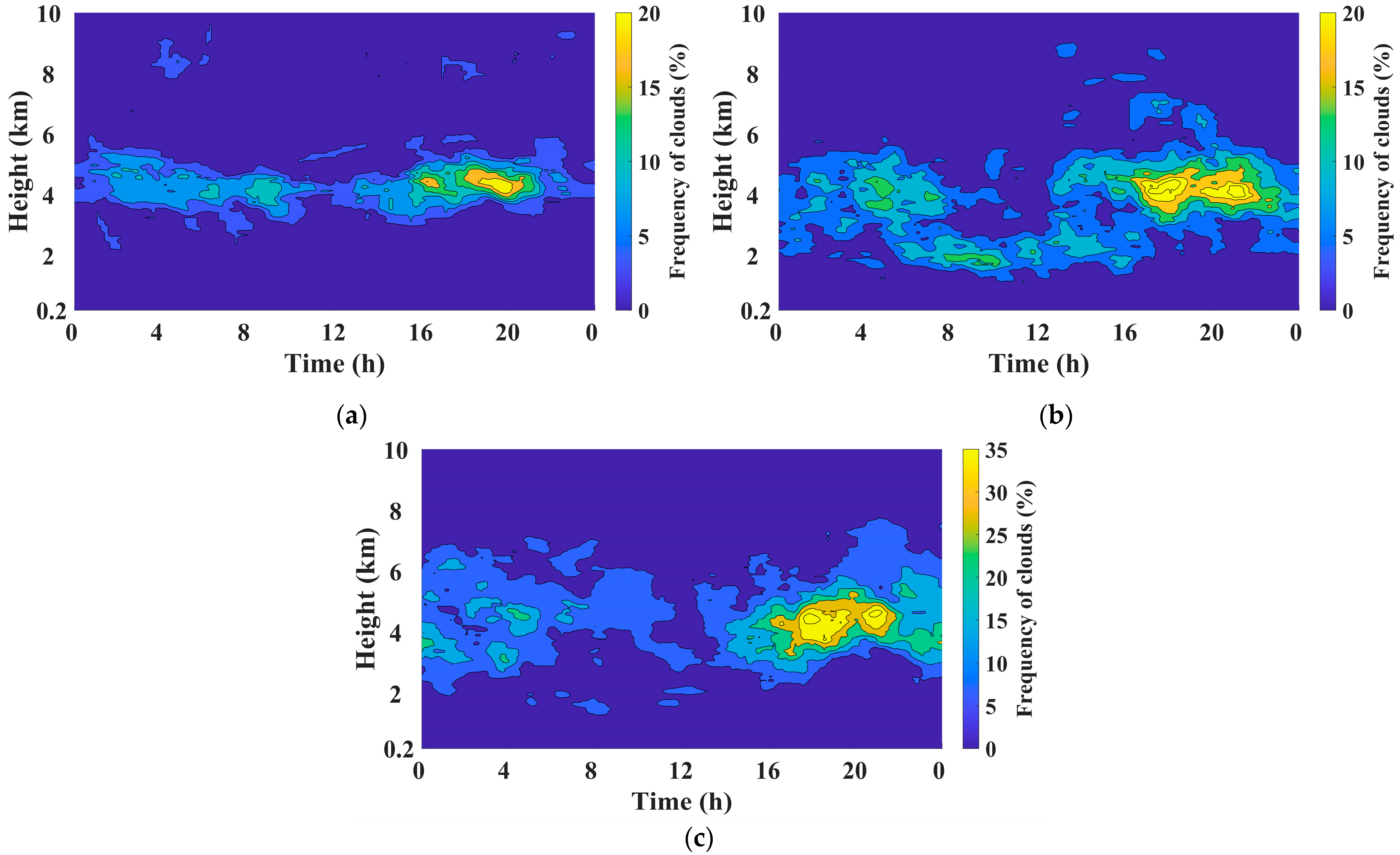
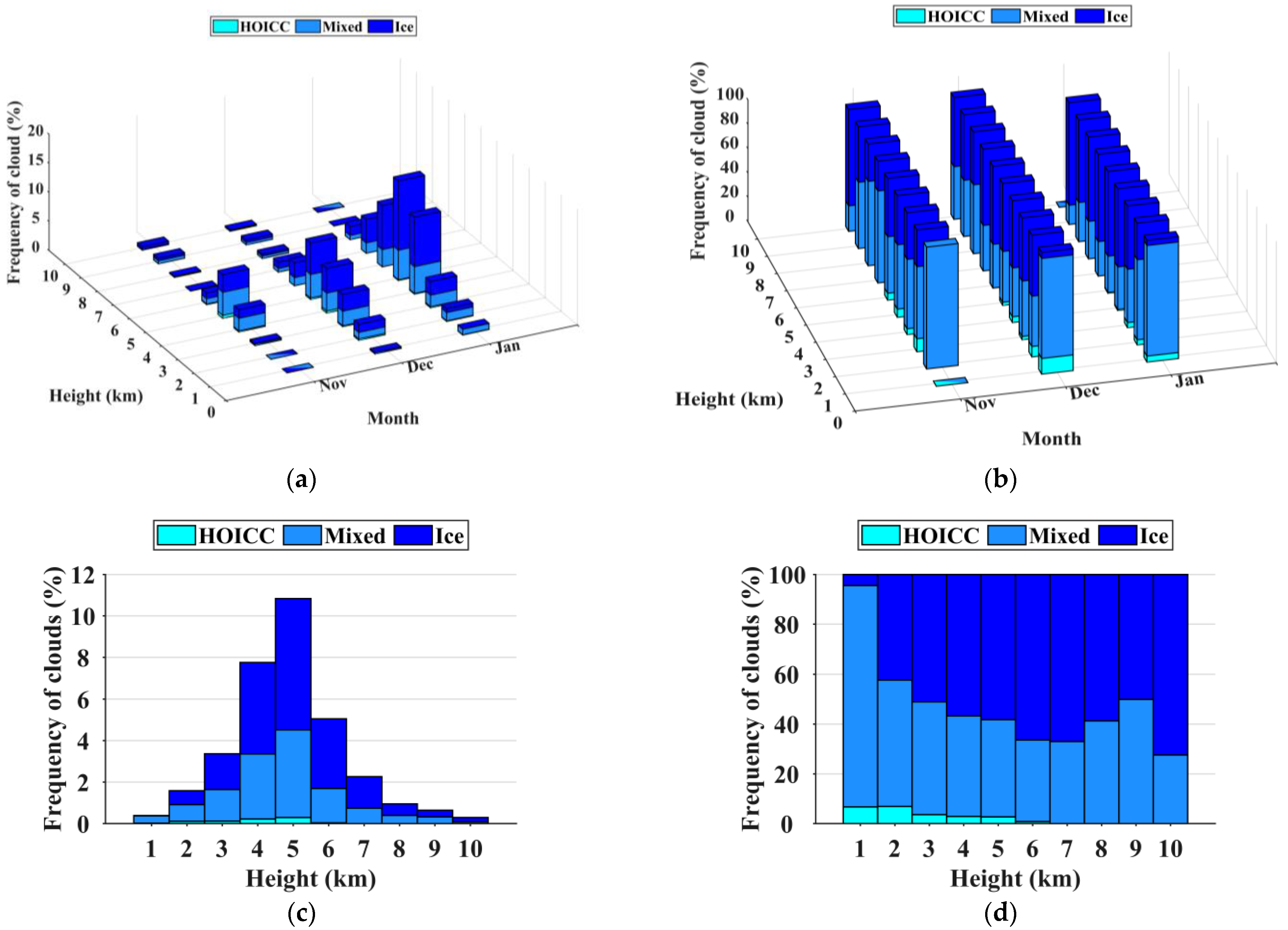
3.1. Characteristics of Cloud Vertical Distribution

According to the classification algorithm described in Section 2.3, the vertical distribution of clouds in Lhasa during the effective observation period was obtained. Because the strong attenuation of clouds can cause a sharp drop in the SNR, we eliminated data with an SNR below 10. In addition, the receiving field of view of the lidar is less than 1 mrad, which can effectively reduce the receiving of multiple scattered signals. Figure 1 shows the average diurnal variations of cloud appearance frequency in different months. We marked the locations identified as clouds in the observation data matrix as 1 and the other locations as 0 to obtain the marker matrix. The sum of the daily marker matrix is divided by the number of days to obtain the average diurnal variations of cloud appearance frequency. In November 2021, the height of the cloud was concentrated at 3–6 km, and the time of appearance was concentrated at 2:00~10:00 Beijing Time (BJT, Universal Time Coordinated + 8 h) and 16:00~22:00 BJT, with the highest appearance frequency of ~23%. In December 2021, the height of cloud appearance was concentrated at the height of 1.5~3 km during the period of 6:00~16:00, but it was at 3 km~6 km during time segments of 4:00~8:00 BJT and 16:00~22:00 BJT, with the highest appearance frequency of ~29%. In January 2022, the height of the cloud appearance was concentrated between 2~7 km during the time period of 16:00~22:00 BJT. During the observation period, the maximum of cloud appearance frequency was 41% in January 2022. The clouds occurred almost all day in December 2021, presenting a different diurnal pattern of cloud appearance frequency from that in the other two months. Multi-layer clouds appeared in the early morning and afternoon in December 2021.

On average, almost no clouds appeared around noon during the field campaign (Figure 2a). The heights of the cloud layer were primarily in the range of 2~7 km, although there were clouds below 2 km. The frequency of cloud appearance between 14:00~22:00 was significantly higher than that at the other time of the day, which is similar to the results reported in previous research studies [2,34]. The peak frequency (~29%) of cloud appearance was significantly lower than that at the same region in summer [2,32]. This is probably related to the cold and dry climate conditions in winter. The water clouds were not identified, probably due to the fact that the temperature was below zero at the height of the cloud appearance in winter of Lhasa. HOICC appeared below 5 km, with an occurrence probability below 1.5% during the observation period (Figure 2b). The proportion of HOICC in ice clouds was close to the global research result reported by Noel et al. [41]. The occurrence probability of mixed cloud was less than 10% in the height range of 1~6 km, mainly around 20:00 BJT (Figure 2c). It should be mentioned that the mixed clouds probably included the supercooled water clouds due to limitations in cloud classification methods. The ice clouds mainly occurred from 16:00 BJT to 22:00 BJT, with maximum frequency at a height of 3–5 km (Figure 2d). The occurrence time of ice clouds is similar to that observed in summer in the Naqu region [2], which is about 200 km away from Lhasa. However, the mean height for the maximum frequency of ice cloud appearance is lower by 3 km in winter in Lhasa, probably due to the seasonal difference in surface radiation.

Figure 3a shows the frequencies of cloud phases at different heights in three months. The frequencies for each cloud phase first increased and then decreased with the increasing heights, and the peak frequency appeared at 5 km. The frequencies of clouds also increased significantly from November 2021 to January 2022. Figure 3b shows the proportions of different cloud phases in the total cloud at different heights in three months. The proportion of mixed clouds showed a decreasing trend with increasing height from November 2021 to January 2022, while the situation was the opposite for the proportion of ice clouds. On average, the maximum of total cloud frequency was ~11% at the 5 km height, dominated by mixed clouds and ice clouds (Figure 3c). At the 1 km height, mixed clouds accounted for 90%, with the remaining 10% for ice clouds and HOICC (Figure 3d). In addition, the maximum proportion (~70%) of ice clouds appeared at 10 km during the field campaign. Only mixed clouds and ice clouds were found above a height of 6 km.

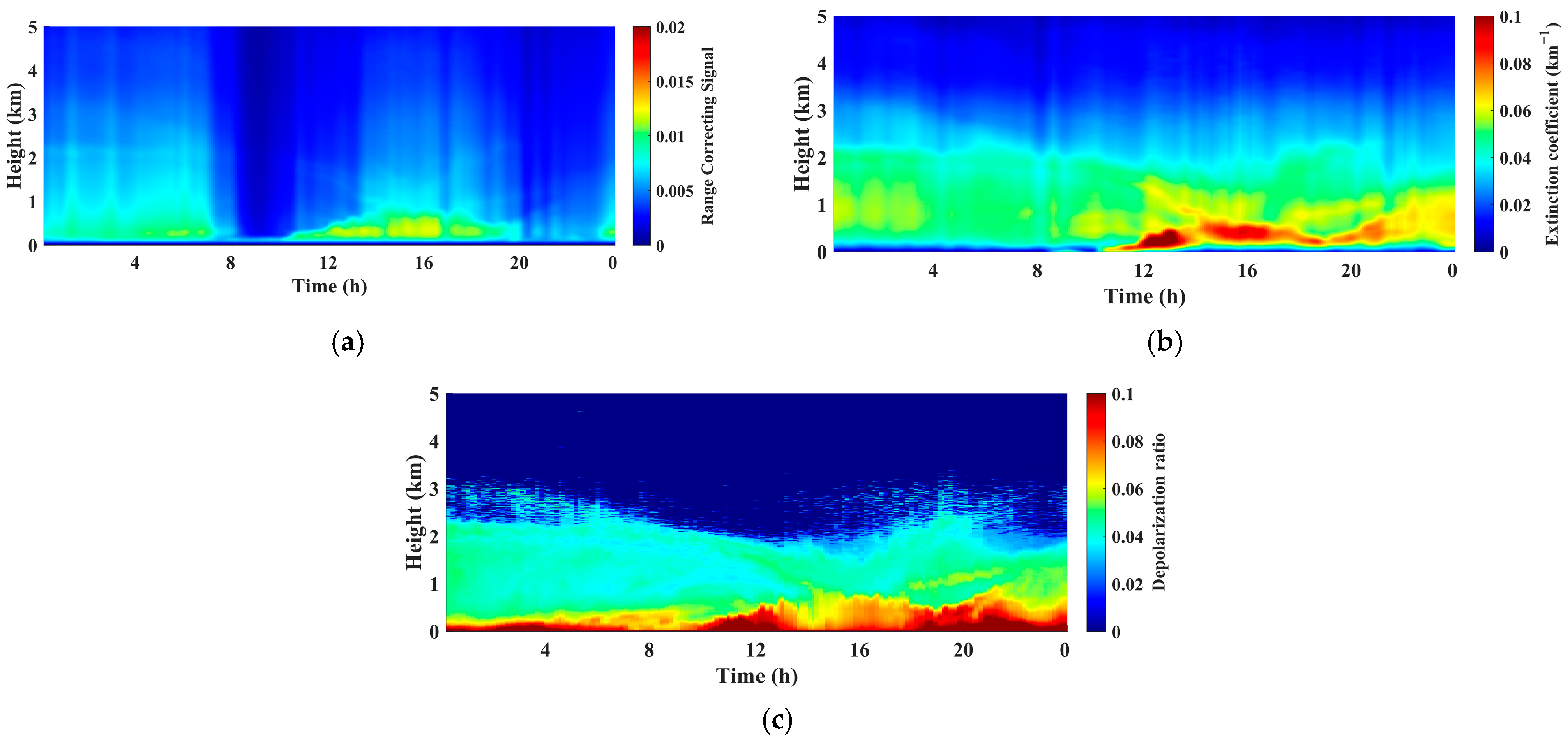
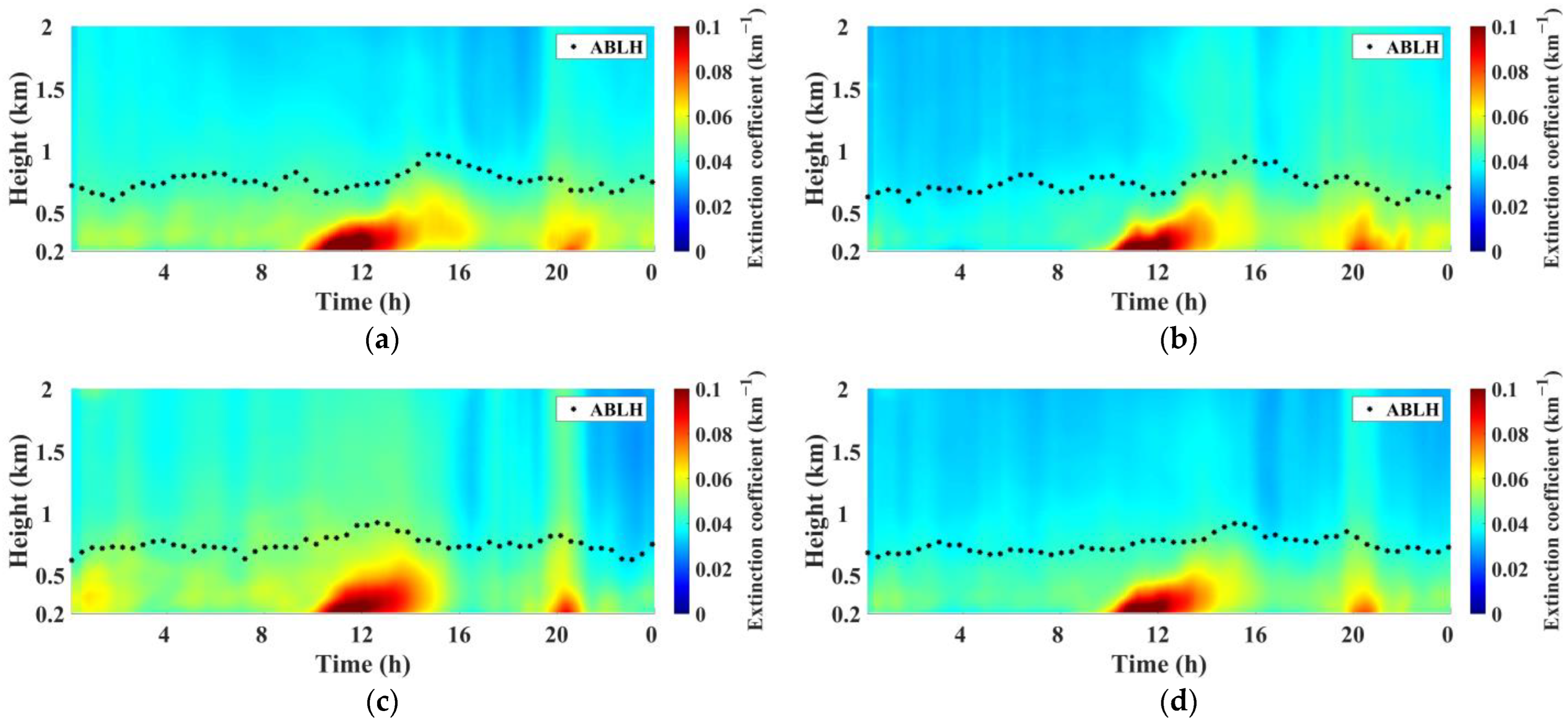
3.2. Monthly and Diurnal Variations of Vertical Distribution of Aerosol Optical Properties

The extinction coefficient and depolarization ratio are affected by different physicochemical properties and aerosol sources [5]. The relationship between aerosol extinction coefficient and PM_2.5 concentration can be simply expressed as ${\mathrm{\alpha }}_{\mathrm{a}}=\mathrm{K}\times {\mathrm{C}}_{\mathrm{p}\mathrm{m}2.5}$ [42]. The specific coefficient K is related to aerosol size distribution, refractive index, and atmospheric relative humidity. When the relative humidity is below 70%, the aerosol hydrophilic growth could be negligible. So, the specific coefficient K could be considered as constant under the condition of less than 70% relative humidity in the planetary boundary layer [42]. In order to verify the reliability of lidar observation in Lhasa, we performed a linear regression analysis between the extinction coefficient in the near-surface layer (i.e., 200–250 m in this study) and the PM_2.5 mass concentration measured at the adjacent station during the field campaign. As shown in Figure 4, the correlation coefficient is 0.77 between them, partly implying that the lidar observations are reliable.

Given the low SNR of the echo signal in the vertical channel above 3 km, we mainly analyzed the vertical evolutions of aerosol optical parameters below 3 km. The data of extinction coefficient and depolarization ratio were rejected once they were affected by the clouds or outside three times the standard deviation in the following statistical analysis. Figure 5 shows the vertical profiles of the extinction coefficient and depolarization ratio in each month as well as during the whole observation period. Both the extinction coefficient and depolarization ratio decreased with increasing altitude. For example, the extinction coefficients were 0.059 ± 0.03 in November 2021, 0.067 ± 0.03 in December 2021, and 0.065 ± 0.08 in January 2022 at 200 m, respectively. The corresponding extinction coefficients at 1 km were 0.043 ± 0.004, 0.047 ± 0.01 and 0.048 ± 0.03, respectively. This indicates that the rather low aerosol concentrations in Lhasa decreased with increasing altitude. In addition, there were no significant monthly trends for the extinction coefficient and depolarization ratio, indicating no significant differences in particle shapes and aerosol sources.

Figure 6 shows the average diurnal variations of the aerosol extinction coefficient and the depolarization ratio in the lower layer (i.e., between 200–400 m) in each month and during the whole observation period. The diurnal variations of the extinction coefficient presented a “double-peak” pattern, around 12:00 BJT and 20:00 BJT, respectively. The averaged diurnal variation of ground PM_2.5 concentration measured at the adjacent monitoring station also presented double peaks, which appeared around 10:00 BJT and 20:00 BJT, respectively (Figure A2). The diurnal cycles were partly influenced by the local source emissions, such as production activities and religious activities [43]. The time differences for the first peak between aerosol extinction and PM_2.5 concentrations were partly related to the particle transport from the lower layer to the higher layer with the development of the boundary layer. The change in the depolarization ratio and extinction coefficient in November 2021 (Figure 6a) and December 2021 (Figure 6b) is consistent, but this consistency is not obvious in January 2022 (Figure 6c). Overall, the diurnal patterns of depolarization ratio were similar to that of aerosol extinction coefficient. Considering the depolarization ratio variation in the range of 0.06–0.1, the rather small fluctuation indicates that the type of aerosol particles did not change significantly during the observation period.

The atmospheric boundary layer height (ABLH) was also retrieved from lidar echo signals by the gradient-based method [44,45,46]. The aerosol lidar-derived ABLH is actually the height of the surface aerosol layer [47]. Assuming that the distribution of aerosol concentration during the daytime is primarily influenced by turbulent mixing, the boundary layer height measured by lidar is considered as the mixed layer height (MLH), which is equivalent to the convective boundary layer height obtained from radiosonde observations [47,48]. For the stable nocturnal boundary layer (NBL), the height determined by aerosol lidar is either the top of the residual layer or the top of the surface mechanical driven ML (MLH, or the height of ground inversion layer) [47]. Figure 7 shows the diurnal variations of ABLH overlaid onto that of the extinction coefficient profile. It is clearly shown that the aerosols were basically distributed within the atmospheric boundary layer (ABL). The ABLH gradually increased from hundreds of meters at ~10:00 BJT to 1 km at ~15:00 BJT. Such ABL development driven by the increase of surface thermal radiation during the day led to the vertical diffusion of aerosols and played an important role in the dilution effect of air pollution. For another air pollution period (around 20:00 BJT), the ABLHs were about 0.6 km and remained nearly at the same level for several hours, which were not conducive to the diffusion of air pollution. In addition, the ABLH diurnal variation pattern did not change significantly over the months during the field campaign.

4. Discussion

Here we report for the first time long continuous lidar observations in Lhasa during winter. The lidar observation shows that the cloud height in winter of Lhasa is significantly lower than that in summer, which is partly related to the weaker thermal force caused by the weakening surface radiation in winter [2]. The clouds always appear except around noon, which is probably related to the local boundary layer processes [49]. The frequency of cloud appearance is also significantly lower in winter than that in summer, which is probably connected with the colder and drier climate conditions in winter. In addition, the clouds in winter of Lhasa are dominated by ice clouds and mixed clouds. Due to the limitations of the cloud classification method and uncertainties of temperature data, almost no water clouds were identified. Probably, there were super-cooled water clouds that were not distinguishable. In addition, the uncertainty of the inversion results caused by multiple scattering and the strong extinction effect of clouds needs further study.

The consistency between aerosol extinction coefficient and PM_2.5 concentrations partially indicates that the lidar observation was reliable during the field campaign. Overall, the extinction coefficients decrease with increasing altitude and the depolarization ratios vary over a small range, indicating that aerosol particles are mainly concentrated in the lower layer and the aerosol type does not change significantly. Thus, the primary sources of aerosol in Lhasa are dominated by local emissions [50]. The clear bimodal structure of aerosol diurnal variation reveals that we should pay more attention to the reduction of local source emissions in the two key periods. In addition, the diurnal variation of the aerosol vertical profile presents a clear diffusion process of aerosols with increasing ABLH, which implies that the ABL evolutions play an important role in air pollution in Lhasa.

5. Conclusions

Lidar observations were performed from November 2021 to January 2022 in Lhasa, one of the major cities on the TP. We identified clouds based on the distance-corrected echo signal of lidar and classified clouds into water clouds, HOICC, mixed clouds, and ice clouds. Then, we investigated the temporal variations of the vertical distribution for each cloud phase. We found that the distribution height and frequency of clouds were significantly different from those reported in summer. We also presented temporal variations of the vertical distribution of aerosol optical properties as well as ABLH retrieved from lidar observation. The main conclusions are as follows:

• Clouds always appeared except around noon during the field campaign, concentrated at a height of about 5 km. The height and frequency of cloud appearance in this study were significantly lower than that reported in summer. The cloud types are dominated by mixed clouds and ice clouds in the winter of Lhasa. The relative proportions of mixed clouds gradually decrease with increasing altitude, but the situation is opposite for ice clouds.
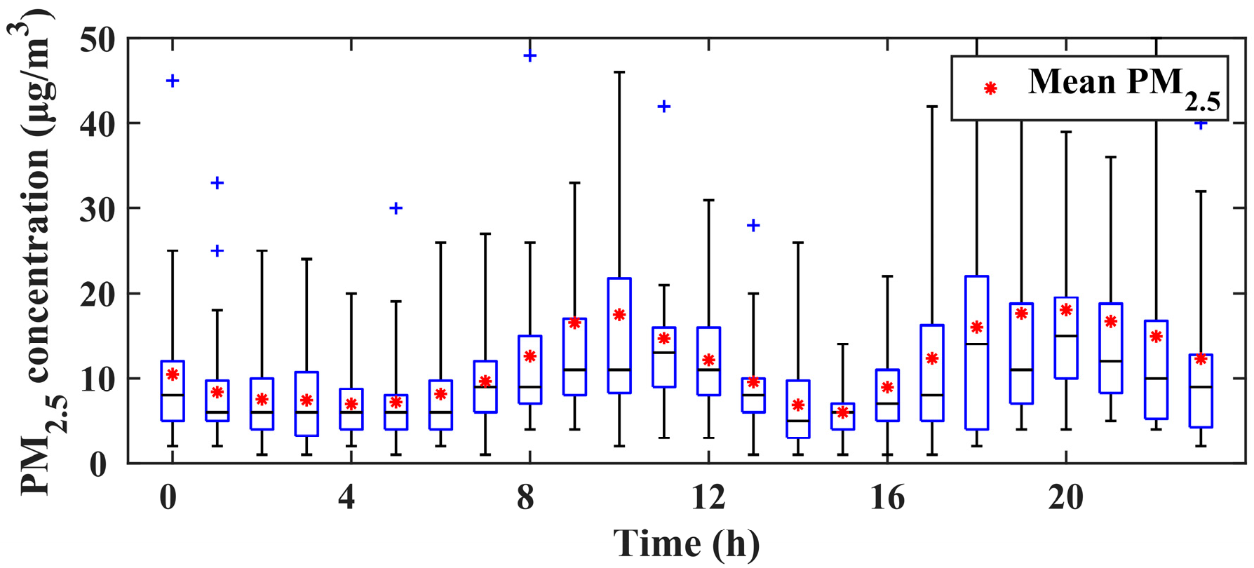
• The aerosol extinction coefficients decrease with increasing altitude. The depolarization ratios vary in the range of 0.06–0.1, implying that the major sources of aerosol particles did not change significantly during the observation period. There were two peaks for aerosol diurnal variation, appearing in the morning and late afternoon, respectively. The aerosols were basically distributed within the ABL. With the ABL development in the morning, the aerosol particles continued to diffuse upward for about 4 h until reaching a height of 1 km at ~15:00 BJT. For another air pollution period (around 20:00 BJT), the ABLHs were about 0.6 km and remained basically at the same level, which is not conducive to the diffusion of air pollution. In addition, the ABLH diurnal variation pattern changed slightly over the months during the field campaign.

As a whole, the results above enhance the understanding of the characteristics of clouds and aerosols in winter over the TP. In the future, the comparisons made by different observation methods will be significant. Also, it is necessary to undertake long-term continuous observations by lidar in different regions of the TP in order to increase the spatial–temporal representativeness.

References

1. Pruppacher, H.R.; Klett, J.D. Microstructure of Atmospheric Clouds and Precipitation. In Microphysics of Clouds and Precipitation, 2nd ed.; Springer: Dordrecht, The Netherlands, 2010; Volume 18, pp. 10–73. [Google Scholar]
2. Bian, Y.; Liu, L.; Zheng, J.; Wu, S.; Dai, G. Classification of Cloud Phase Using Combined Ground-Based Polarization Lidar and Millimeter Cloud Radar Observations Over the Tibetan Plateau. IEEE Trans. Geosci. Remote Sens. 2023, 61, 1–13. [Google Scholar] [CrossRef]
3. Yin, Y.; Wurzler, S.; Levin, Z.; Reisin, T.G. Interactions of mineral dust particles and clouds: Effects on precipitation and cloud optical properties. J. Geophys. Res.-Atmos. 2002, 107, AAC 19-1–AAC 19-14. [Google Scholar] [CrossRef]
4. Twomey, S. Aerosols, clouds and radiation. Atmos. Environ. 1991, 25, 2435–2442. [Google Scholar] [CrossRef]
5. Li, M.; Cao, X.; Zhang, Z.; Ji, H.; Zhang, M.; Guo, Y.; Tian, P.; Liang, J. Optical Properties and Vertical Distribution of Aerosols Using Polarization Lidar and Sun Photometer over Lanzhou Suburb in Northwest China. Remote Sens. 2023, 15, 4927. [Google Scholar] [CrossRef]
6. Xu, X.; Lu, C.; Shi, X.; Gao, S. World water tower: An atmospheric perspective. Geophys. Res. Lett. 2008, 35, L20815. [Google Scholar] [CrossRef]
7. Qiu, J. China: The third pole. Nature 2008, 454, 393–396. [Google Scholar] [CrossRef] [PubMed]
8. Lau, W.K.M.; Kim, M.; Kim, K.; Lee, W. Enhanced surface warming and accelerated snow melt in the Himalayas and Tibetan Plateau induced by absorbing aerosols. Environ. Res. Lett. 2010, 5, 25204. [Google Scholar] [CrossRef]
9. Yu, R.; Wang, B.; Zhou, T. Climate Effects of the Deep Continental Stratus Clouds Generated by the Tibetan Plateau. J. Clim. 2004, 17, 2702–2713. [Google Scholar] [CrossRef]
10. Duan, A.; Wu, G. Change of cloud amount and the climate warming on the Tibetan Plateau. Geophys. Res. Lett. 2006, 33, L22704. [Google Scholar] [CrossRef]
11. Duo, B.; Cui, L.; Wang, Z.; Li, R.; Zhang, L.; Fu, H.; Chen, J.; Zhang, H.; Qiong, A. Observations of atmospheric pollutants at Lhasa during 2014–2015: Pollution status and the influence of meteorological factors. J. Environ. Sci. 2018, 63, 28–42. [Google Scholar] [CrossRef]
12. Ran, L.; Lin, W.L.; Deji, Y.Z.; La, B.; Tsering, P.M.; Xu, X.B.; Wang, W. Surface gas pollutants in Lhasa, a highland city of Tibet -current levels and pollution implications. Atmos. Chem. Phys. 2014, 14, 10721–10730. [Google Scholar] [CrossRef]
13. Cui, Y.Y.; Liu, S.; Bai, Z.; Bian, J.; Li, D.; Fan, K.; McKeen, S.A.; Watts, L.A.; Ciciora, S.J.; Gao, R. Religious burning as a potential major source of atmospheric fine aerosols in summertime Lhasa on the Tibetan Plateau. Atmos. Environ. 2018, 181, 186–191. [Google Scholar] [CrossRef]
14. Shang, H.; Letu, H.; Nakajima, T.; Wang, Z.; Ma, R.; Wang, T.; Lei, Y.; Ji, D.; Li, S.; Shi, J. Diurnal cycle and seasonal variation of cloud cover over the Tibetan Plateau as determined from Himawari-8 new-generation geostationary satellite data. Sci. Rep. 2018, 8, 1105. [Google Scholar] [CrossRef]
15. Yan, Y.; Liu, Y.; Lu, J. Cloud vertical structure, precipitation, and cloud radiative effects over Tibetan Plateau and its neighboring regions. J. Geophys. Res.-Atmos. 2016, 121, 5864–5877. [Google Scholar] [CrossRef]
16. Liu, Z.; Liu, D.; Huang, J.; Vaughan, M.; Uno, I.; Sugimoto, N.; Kittaka, C.; Trepte, C.; Wang, Z.; Hostetler, C. Airborne dust distributions over the Tibetan Plateau and surrounding areas derived from the first year of CALIPSO lidar observations. Atmos. Chem. Phys. 2008, 8, 5045–5060. [Google Scholar] [CrossRef]
17. Bian, Y.; Xu, W.; Hu, Y.; Tao, J.; Kuang, Y.; Zhao, C. Method to retrieve aerosol extinction profiles and aerosol scattering phase functions with a modified CCD laser atmospheric detection system. Opt. Express 2020, 28, 6631–6647. [Google Scholar] [CrossRef] [PubMed]
18. Sassen, K. The Polarization Lidar Technique for Cloud Research: A Review and Current Assessment. Bull. Amer. Meteorol. Soc. 1991, 72, 1848–1866. [Google Scholar] [CrossRef]
19. Bohlmann, S.; Shang, X.; Vakkari, V.; Giannakaki, E.; Leskinen, A.; Lehtinen, K.E.J.; Atsi, S.P.; Komppula, M. Lidar depolarization ratio of atmospheric pollen at multiple wavelengths. Atmos. Chem. Phys. 2021, 21, 7083–7097. [Google Scholar] [CrossRef]
20. Vakkari, V.; Baars, H.; Bohlmann, S.; Uhl, J.B.; Komppula, M.; Mamouri, R.E.; O’Connor, E.J. Aerosol particle depolarization ratio at 1565nm measured with a Halo Doppler lidar. Atmos. Chem. Phys. 2021, 21, 5807–5820. [Google Scholar] [CrossRef]
21. Dai, G.; Wu, S.; Song, X. Depolarization Ratio Profiles Calibration and Observations of Aerosol and Cloud in the Tibetan Plateau Based on Polarization Raman Lidar. Remote Sens. 2018, 10, 378. [Google Scholar] [CrossRef]
22. Jia, R.; Liu, Y.; Chen, B.; Zhang, Z.; Huang, J. Source and transportation of summer dust over the Tibetan Plateau. Atmos. Environ. 2015, 123, 210–219. [Google Scholar] [CrossRef]
23. Yin, X.; de Foy, B.; Wu, K.; Feng, C.; Kang, S.; Zhang, Q. Gaseous and particulate pollutants in Lhasa, Tibet during 2013-2017: Spatial variability, temporal variations and implications. Environ. Pollut. 2019, 253, 68–77. [Google Scholar] [CrossRef] [PubMed]
24. Cheng, S.; Pu, G.; Ma, J.; Hong, H.; Du, J.; Yudron, T.; Wagner, T. Retrieval of Tropospheric NO2 Vertical Column Densities from Ground-Based MAX-DOAS Measurements in Lhasa, a City on the Tibetan Plateau. Remote Sens. 2023, 15, 4869. [Google Scholar] [CrossRef]
25. Lv, L.; Liu, W.; Zhang, T.; Chen, Z.; Dong, Y.; Fan, G.; Xiang, Y.; Yao, Y.; Yang, N.; Chu, B. Observations of particle extinction, PM2.5 mass concentration profile and flux in north China based on mobile lidar technique. Atmos. Environ. 2017, 164, 360–369. [Google Scholar] [CrossRef]
26. Fernald, F.G.; Herman, B.M.; Reagan, J.A. Determination of Aerosol Height Distributions by Lidar. J. Appl. Meteorol. Climatol. 1972, 11, 482–489. [Google Scholar] [CrossRef]
27. Collis, R.T.H.; Russell, P.B. Lidar measurement of particles and gases by elastic backscattering and differential absorption. In Laser Monitoring of the Atmosphere; Hinkley, E.D., Ed.; Springer: Berlin, Germany, 1976; Volume 14, pp. 71–151. [Google Scholar]
28. Klett, J.D. Stable analytical inversion solution for processing lidar returns. Appl. Optics 1981, 20, 211–220. [Google Scholar] [CrossRef]
29. Fernald, F.G. Analysis of atmospheric lidar observations: Some comments. Appl. Optics 1984, 23, 652–653. [Google Scholar] [CrossRef] [PubMed]
30. Wiegner, M.; Groß, S.; Freudenthaler, V.; Schnell, F.; Gasteiger, J. The May/June 2008 Saharan dust event over Munich: Intensive aerosol parameters from lidar measurements. J. Geophys. Res.-Atmos. 2011, 116, D23213. [Google Scholar] [CrossRef]
31. Mattis, I.; Ansmann, A.; Müller, D.; Wandinger, U.; Althausen, D. Dual-wavelength Raman lidar observations of the extinction-to-backscatter ratio of Saharan dust. Geophys. Res. Lett. 2002, 29, 20–1–20–4. [Google Scholar] [CrossRef]
32. National Geophysical Data Center. U.S. standard Atmosphere (1976). Planet Space Sci. 1992, 40, 553–554. [Google Scholar] [CrossRef]
33. Redemann, J.; Turco, R.P.; Pueschel, R.F.; Fenn, M.A.; Browell, E.V.; Grant, W.B. A multi-instrument approach for characterizing the vertical structure of aerosol properties: Case studies in the Pacific Basin troposphere. J. Geophys. Res.-Atmos. 1998, 103, 23287–23298. [Google Scholar] [CrossRef]
34. Su, J.; Liu, Z.; Wu, Y.; Mc Cormick, M.P.; Lei, L. Retrieval of multi-wavelength aerosol lidar ratio profiles using Raman scattering and Mie backscattering signals. Atmos. Environ. 2013, 79, 36–40. [Google Scholar] [CrossRef]
35. Freudenthaler, V.; Esselborn, M.; Wiegner, M.; Heese, B.; Tesche, M.; Ansmann, A.; Müller, D.; Althausen, D.; Wirth, M.; Fix, A. Depolarization ratio profiling at several wavelengths in pure Saharan dust during SAMUM 2006. Tellus Ser. B-Chem. Phys. Meteorol. 2009, 61, 165–179. [Google Scholar] [CrossRef]
36. Zhao, C.; Wang, Y.; Wang, Q.; Li, Z.; Wang, Z.; Liu, D. A new cloud and aerosol layer detection method based on micropulse lidar measurements. Atmos. Chem. Phys. 2014, 119, 6788–6802. [Google Scholar] [CrossRef]
37. Insperger, T.; Stépán, G. Semi-discretization. In Semi-Discretization for Time-Delay Systems: Stability and Engineering Applications; Springer: New York, NY, USA, 2011; Volume 178, pp. 39–71. [Google Scholar]
38. Clothiaux, E.E.; Mace, G.G.; Ackerman, T.P.; Kane, T.J.; Spinhirne, J.D.; Scott, V.S. An Automated Algorithm for Detection of Hydrometeor Returns in Micropulse Lidar Data. J. Atmos. Ocean. Technol. 1998, 15, 1035–1042. [Google Scholar] [CrossRef]
39. Campbell, J.R.; Sassen, K.; Welton, E.J. Elevated Cloud and Aerosol Layer Retrievals from Micropulse Lidar Signal Profiles. J. Atmos. Ocean. Technol. 2008, 25, 685–700. [Google Scholar] [CrossRef]
40. Hersbach, H.; Bell, B.; Berrisford, P.; Biavati, G.; Horányi, A.; Muñoz Sabater, J.; Nicolas, J.; Peubey, C.; Radu, R.; Rozum, I.; et al. ERA5 Hourly Data on Pressure Levels from 1940 to Present. Copernicus Climate Change Service (C3S) Climate Data Store (CDS). 2023. Available online: https://cds.climate.copernicus.eu/cdsapp#!/dataset/reanalysis-era5-pressure-levels?tab=overview (accessed on 7 January 2024).
41. Noel, V.; Chepfer, H. A global view of horizontally oriented crystals in ice clouds from Cloud-Aerosol Lidar and Infrared Path finder Satellite Observation (CALIPSO). J. Geophys. Res.-Atmos. 2010, 115, D00H23. [Google Scholar] [CrossRef]
42. Tao, Z.; Wang, Z.; Yang, S.; Shan, H.; Ma, X.; Zhang, H.; Zhao, S.; Liu, D.; Xie, C.; Wang, Y. Profiling the PM2.5 mass concentration vertical distribution in the boundary layer. Atmos. Meas. Tech. 2016, 9, 1369–1376. [Google Scholar] [CrossRef]
43. Li, C.; Han, X.; Kang, S.; Yan, F.; Chen, P.; Hu, Z.; Yang, J.; Ciren, D.; Gao, S.; Sillanpää, M. Heavy near-surface PM2.5 pollution in Lhasa, China during a relatively static winter period. Chemosphere 2019, 214, 314–318. [Google Scholar] [CrossRef] [PubMed]
44. Vivone, G.; D’Amico, G.; Summa, D.; Lolli, S.; Amodeo, A.; Bortoli, D.; Pappalardo, G. The Contribution of Local Anthropogenic Emissions to Air Pollutants in Lhasa on the Tibetan Plateau. Atmos. Chem. Phys. 2021, 21, 4249–4265. [Google Scholar] [CrossRef]
45. Flamant, C.; Pelon, J.; Flamant, P.H.; Durand, P. Lidar Determination of The Entrainment Zone Thickness at the Top of the Unstable Marine Atmospheric Boundary Layer. Bound.-Layer Meteor. 1997, 83, 247–284. [Google Scholar] [CrossRef]
46. Tsaknakis, G.; Papayannis, A.; Kokkalis, P.; Amiridis, V.; Kambezidis, H.D.; Mamouri, R.E.; Georgoussis, G.; Avdikos, G. Inter-comparison of lidar and ceilometer retrievals for aerosol and Planetary Boundary Layer profiling over Athens, Greece. Atmos. Meas. Tech. 2011, 4, 1261–1273. [Google Scholar] [CrossRef]
47. Dang, R.; Yang, Y.; Hu, X.; Wang, Z.; Zhang, S. A Review of Techniques for Diagnosing the Atmospheric Boundary Layer Height (ABLH) Using Aerosol Lidar Data. Remote Sens. 2019, 11, 1590. [Google Scholar] [CrossRef]
48. Dang, R.; Yang, Y.; Li, H.; Hu, X.; Wang, Z.; Huang, Z.; Zhou, T.; Zhang, T. Atmosphere Boundary Layer Height (ABLH) Determination under Multiple-Layer Conditions Using Micro-Pulse Lidar. Remote Sens. 2019, 11, 263. [Google Scholar] [CrossRef]
49. Li, Y.; Zhang, M. Cumulus over the Tibetan Plateau in the Summer Based on CloudSat–CALIPSO Data. J. Clim. 2016, 29, 1219–1230. [Google Scholar] [CrossRef]
50. Chen, S.; Wang, W.; Li, M.; Mao, J.; Ma, N.; Liu, J.; Bai, Z.; Zhou, L.; Wang, X.; Bian, J. Atmospheric boundary layer height estimation from aerosol lidar: A new approach based on morphological image processing techniques. J. Geophys. Res.-Atmos. 2022, 127, e2021JD036202. [Google Scholar] [CrossRef]
Figure 1. Average diurnal variations of cloud appearance frequency in (a) November 2021, (b) December 2021, and (c) January 2022 (BJT).
Remotesensing 16 02074 g001
Figure 2. Diurnal variations of the vertical distribution of cloud frequencies during the field campaign for (a) all clouds, (b) HOICCs, (c) mixed clouds, and (d) ice clouds (BJT).
Remotesensing 16 02074 g002
Figure 3. (a) The frequency of cloud phases at different heights in three months; (b) the proportion of different cloud phases in the total cloud at different heights in three months; (c) the mean frequency of cloud phases at different heights during the observation period; (d) the averaged proportion of different cloud phases in the total cloud at different heights during the observation period (HOICC: cyan; mixed cloud: light blue; ice cloud: blue).
Remotesensing 16 02074 g003
Figure 4. Linear regression analysis between the hourly extinction coefficient at the height range of 200~250 m and corresponding PM2.5 mass concentration measured at the adjacent station during the field campaign.
Remotesensing 16 02074 g004
Figure 5. Mean vertical profiles of extinction coefficient (upper panel) and depolarization ratio (lower panel) (a,e) in November 2021, (b,f) in December 2021, (c,g) in January 2022, and (d,h) during the whole observation period (BJT). The error bars indicate the standard deviations.
Remotesensing 16 02074 g005
Figure 6. Diurnal variations of extinction coefficient and depolarization ratio between 200–400 m in (a) November 2021, (b) December 2021, (c) January 2022, and (d) during the whole observation period (BJT).
Remotesensing 16 02074 g006
Figure 7. Diurnal variations of extinction coefficient profile and ABLH (black dot line) in (a) November 2021, (b) December 2021, (c) January 2022, and (d) during the whole observation period (BJT).
Remotesensing 16 02074 g007