Multi-Shot Simultaneous Deghosting for Virtual-Shot Gathers via Integrated Sparse and Nuclear Norm Constraint Inversion

Abstract

Seismic interferometry is a key technology in geophysical exploration, having achieved significant developments in constructing virtual seismic responses, overcoming the limitation of traditional exploration. However, non-physical reflections in virtual-shot gathers pose challenges for data processing and interpretation. This study focuses on deghosting in virtual-shot gather data processing. We propose a novel method that integrates sparse and nuclear norm constraint inversion for multi-shot simultaneous deghosting. Initially, a pseudo 3D data cube is created to enhance computational efficiency and lay the foundation for subsequent continuity regularization. Subsequently, an inversion framework is constructed to improve deghosting precision and stability by combining sparse and nuclear norm constraint inversion. Both synthetic and field examples demonstrate the superiority of our method, offering a new paradigm for virtual-shot gather data processing, and representing a major advancement in overcoming the inherent limitations of seismic interferometry.

1. Introduction

Seismic interferometry, a groundbreaking approach in geophysical exploration, has revolutionized our ability to interpret and understand seismic data. Pioneered by Snieder in 2009, this entirely data-driven method allows for the construction of virtual seismic responses between any two receivers, eliminating the need for detailed source information [1]. This technique can convert the seismic signals of two receivers with overlapping propagation paths into a new record, creating a scenario where one receiver acts as a source while the other receives the seismic wave [2]. The significant advantage of seismic interferometry lies in its ability to enhance the flexibility and scope of seismic exploration, overcoming traditional limitations. Its application spans various domains including oil and gas exploration [3,4,5,6,7], mineral exploration [8,9], tectonic structure investigation [10,11], fluid monitoring [12], etc. Its impact is not limited to commercial applications but also extends to academic and environmental studies, proving its versatility and wide-ranging influence.

Although seismic interferometry has achieved substantial progress across various fields, it still faces challenges. Fundamentally, seismic interferometry assumes a complete boundary of sources around the receivers, an assumption that often confronts practical constraints in field applications, particularly due to the limited distribution of surface-based illuminating sources [1]. This discrepancy results in complexities in the wavefield interactions, notably in the generation of non-physical reflections (as shown in Figure 1) due to cross-correlation between diverse interfaces [13]. These non-physical reflections, characterized by kinematic properties similar to actual seismic reflections, represent a form of coherent noise that challenges conventional denoising methods. Their resemblance to true seismic signals makes them difficult to distinguish and remove effectively. Furthermore, these reflections often obscure many reconstructed weak events in the virtual seismic response, creating a potential for instability in subsequent inversion processes. Such attributes of non-physical reflections significantly affect data processing, predominantly due to their contribution to a low signal-to-noise ratio of the data [14,15,16]. This issue is a critical factor in the failure of most conventional processing methods, as outlined by Schuster in his seminal work on seismic interferometry.

To overcome these challenges, there have been significant advancements in techniques such as multiple suppression [17,18], weak signal enhancement [19], and migration methods [20]. These developments aim to refine the processing to effectively address distortions caused by non-physical reflections. Our paper concentrates on deghosting within the context of non-physical reflection interference.

Ghost interference is a common issue in marine seismic exploration, arising from the receivers being positioned at a certain depth below the sea surface [21]. This setup results in the formation of downgoing wavefields from the sea surface that mix with upgoing wavefields from the seabed, captured by the receivers [22]. Ghosts, typically appearing after the primary signal, interfere with it and degrade the data quality. Specifically, they narrow the frequency band of the effective signal and eliminate the low frequencies [23]. Additionally, the phase distortion affects accurate event localization, while reduced data resolution compromises the clarity of seismic interpretation, highlighting the critical need for precise deghosting methods in marine seismic exploration.

The inversion-based deghosting method combines plane wave decomposition with the construction of ghost delay operators and utilizes a linear inversion algorithm to extract ghost-free wavefields, which have been gaining prominence in recent years [24,25]. Recent advances in this field have focused on integrating high-performance inversion algorithms [26,27,28] or machine learning techniques [29,30,31] to further improve deghosting results. Despite these significant advancements, existing deghosting methods does not specifically consider the influence of non-physical reflections of the virtual gathers, which is generated by seismic interferometry.

As mentioned above, non-physical reflections can lead to unstable inversion processes and reduced accuracy in conventional deghosting algorithms. Therefore, we present an innovative deghosting method for the virtual gathers based on the principles of low-rank approximation and sparse inversion. This advanced method aims to improve the stability by enhancing denoising ability and adding prior constraints. To solve the problem of noise interference, we introduced a sparse constraint method to enhance inversion accuracy. Additionally, the proposed method modifies the traditional deghosting mode that involves deghosting shot by shot. Taking advantage of the characteristics of streamer observation systems, the data are rearranged into 3D data cubes, transforming the single-shot inversion into multi-shot inversion. Introducing nuclear norm constraints allows stratigraphic continuity to become a new constraint in the inversion process, further improving the accuracy. Synthetic data and field data are used to verify the effectiveness of the proposed method.

2. Materials and Methods

2.1. Foundational Information

In this section, we will introduce the foundational information. We will present the principles and limitations of the deghosting methods, highlighting the challenges faced by conventional deghosting methods when applied to virtual-shot gathers.

For existing deghosting algorithms, Ghosh demonstrated, through a comparison of deconvolution-based time-domain and frequency-domain deghosting algorithms, that the frequency-domain algorithm is more stable [21]. Furthermore, due to the independence of slowness information from frequency in the frequency–slowness domain, the stability is enhanced [22]. In practical applications, the deghosting algorithm based on a linear Radon transform is the most widely used [24,32]. In this method, seismic records are transformed from the time–space domain to the time–slowness domain through the Radon transform. According to the slowness information, each trace is associated with its corresponding ghost delay time $△t_i$:

$$△t_i=\frac{2z\sqrt{1-p_i^2{v}^2}}{v},$$

(1)

where $p_i$ indicates the different trace slowness in the Radon domain, $z$ is receiver depth, and $v$ is water velocity. The Radon domain deghosting method can be represented as

$$D(x_j,\omega )={\displaystyle {\displaystyle \sum _{i=1}^{np}}S(p_i,\omega )}\cdot e^{-i\omega p_i{x}_j}\cdot (1-e^{-i\omega \Delta t_i}),$$

(2)

where $D(x_j,\omega )$ represent two-dimensional seismic records in the frequency domain;$x_j$ and $\omega$ are the offset index and angular frequency. $S(p_i,\omega )$ represent frequency domain deghosting results, which can be expressed as

$$\left[\begin{array}{c}D(x_1,\omega )\\ D(x_2,\omega )\\ ⋮\\ D(x_{n-1},\omega )\\ D(x_n,\omega )\end{array}\right]=\left[\begin{array}{ccccc}{G}_{1,1}& G_{1,2}& \cdots & G_{1,np-1}& G_{1,np}\\ G_{2,1}& G_{2,2}& \cdots & G_{2,np-1}& G_{2,np}\\ ⋮& ⋮& G_{i,j}& ⋮& ⋮\\ G_{n-1,1}& G_{n-1,2}& \cdots & G_{n-1,np-1}& G_{n-1,np}\\ G_{n,1}& G_{n,2}& \cdots & G_{n,np-1}& G_{n,np}\end{array}\right]\left[\begin{array}{c}S(p_1,\omega )\\ S(p_2,\omega )\\ ⋮\\ S(p_{np-1},\omega )\\ S(p_{np},\omega )\end{array}\right]$$

(3)

where $G_{i,j}=e^{-i\omega p_i{x}_j}\cdot (1-e^{-i\omega \Delta t_i})$. We can simplify this process by using a linear equation for expression, as shown in Equation (4):

$$D=GS,$$

(4)

where $G$ represents a ghost operator. Solving the linear inversion problem can obtain the Radon domain deghosting result, which is expressed as

$$S=(G^{H}G+\epsilon I{)}^{-1}{G}^{H}D.$$

(5)

Finally, performing an inverse Fourier transform in the frequency direction can obtain the time–space domain deghosting results.

However, although such methods have been proven to achieve good results under normal circumstances, they face limitations when dealing with complex wavefields, especially when the data contain a significant amount of noise. As mentioned above, the virtual-shot gathers contain a large amount of non-physical noise, which severely limits the effectiveness of the deghosting inversion.

Virtual-shot gathers are generated through seismic interferometry [33,34]. By processing the original seismic data using seismic interferometry, it can be transformed into the data that approximate being generated from any arbitrary subsurface location. This transformed data are known as virtual-shot gathers. In exploration, the flexibility of interferometry is often used to reposition imaging points to penetrate complex overburdens or enhance illumination. Seismic interferometry is applicable to both active seismic data and passive seismic data (Figure 2). The original data can be transformed into virtual-shot gathers through Equations (6) and (7) [35].

$$\Re \{G(x_B,x_A,\omega )\}\approx \frac{1}{\rho c}{\displaystyle \int G(x_B,S,\omega )G{(x_A,S,\omega )}^{\ast }dS},$$

(6)

$$\Re \{\widehat{G}(x_B,x_A,\omega )\}\widehat{S}(\omega )=\frac{1}{\rho c}〈{\widehat{p}}^{obs}(x_B,S,\omega ){\widehat{p}}^{obs}{(x_A,S,\omega )}^{\ast }〉,$$

(7)

where $\Re$ represents the real part of a complex number; $G$ and ${\widehat{p}}^{obs}$ represent the active and passive seismic wavefield. $\omega$ represents the angular frequency; * denotes the complex conjugate in the frequency domain. $\rho$ is the density and $c$ is the propagation velocity, and $〈\cdot 〉$ represents the overall spatial average.

The process of seismic interferometry can be understood as the matching of different wavefield propagation paths. The cross-correlation process cancels the overlapping paths, approximating the data as a new wavefield. However, unmatched wavefield paths during cross-correlation generate non-physical noise [20]. This non-physical noise presents a major challenge for deghosting frameworks when dealing with virtual-shot gathers, introducing perturbations that disrupt the propagation relationship between the primary and ghost, thereby affecting the stability of the inversion process.

2.2. Multi-Shots’ Sparse Inversion with Nuclear Norm Constraint Deghosting Framework

To overcome this challenge, we propose a novel inversion deghosting framework. We introduce sparse constraints to reduce the impact of non-physical noise along the shot direction. Additionally, the nuclear norm constraints are introduced, allowing the continuity of the layer along the offset direction to serve as a new prior constraint, thereby enhancing the stability of the inversion. In this section, we first introduce how to construct the joint inversion framework based on sparse constraints and nuclear norm constraints. We then provide a comprehensive data processing workflow, including the preprocessing steps for obtaining a 3D data cube suited for joint sparse and nuclear norm constraints, as well as the solution methods for the joint constraint inversion.

2.2.1. Joint Inversion Framework with Sparse and Nuclear Norm Constraints

We regard the challenge as an inversion problem. Applying regularization during the inversion process can prevent data overfitting and reduce its complexity with respect to noise, thereby enhancing the stability of the inversion [36]. Considering the characteristics of the data, in this paper, we choose a sparse constraint and nuclear norm constraint as regularization terms to optimize the inversion process.

Sparse inversion, rooted in compressive sensing theory, aims to discretize the seismic signal using a sampling matrix to eliminate redundant information [37]. By integrating sparse inversion algorithms with deghosting frameworks, the influence of non-physical events can be suppressed. Additionally, to further enhance the stability of the inversion process, introducing new prior constraints is proven to be an effective strategy. Lateral continuity of layers can be a good choice that can reduce the non-uniqueness of the solution, making the inversion results more stable and reliable [38]. Nuclear norm regularization treats the seismic reflection coefficient matrix as a low-rank matrix, and by minimizing its nuclear norm, lateral constraints are applied, which can achieve the goal of the incorporation of lateral stratigraphic continuity as a prior constraint into the inversion process [39,40].

The inversion process with regularization constraints can be expressed by Equation (8):

$$F\left(r\right)={‖Wr-D‖}_q+\phi R(r),$$

(8)

where $r$ is the inversion result, $D$ is the input data, and $W$ is the observation matrix. ${‖Wr-D‖}_q$ represents the data fitting term, $\phi R(r)$ is the regularization term, and $\phi$ is the parameter controlling the strength of the regularization.

In the deghosting inversion, the observation matrix is equal to the ghost operator $G$, and the inversion result is deghosting data $S$. Therefore, we can construct the deghosting inversion framework with regularization constraints by rewriting Equation (8):

$$F\left(S\right)={‖GS-D‖}_q+\phi R(S),$$

(9)

and when using sparse constraint as the regularization method, Equation (9) can be rewritten as follows (see Appendix A for details):

$$F\left(S\right)={‖GS-D‖}_2^2+\lambda {‖S‖}_1,$$

(10)

where ${‖\cdot ‖}_1$ represents the L1 norm of the pure signal; ${‖\cdot ‖}_2^2$ denotes the calculation of the squares of the L2 norm, which is the sum of the squares of the vector elements. It should be noted that Equation (11) is the equation of single-shot inversion. When we extend the inversion from single-shot to multi-shot simultaneous inversion, Equation (10) can be rewritten as

$$F\left(S\right)={‖GS-D‖}_F^2+\lambda {‖S‖}_1,$$

(11)

where ${‖\cdot ‖}_F^2$ represents the squares of the Frobenius norm, that is, the sum of the squares of the matrix elements.

When using nuclear norm constraints as a regularization method, Equation (9) is rewritten as follows (detailed content can be found in Appendix B):

$$F\left(S\right)={‖GS-D‖}_F^2+\mu {‖S‖}_{\ast },$$

(12)

where ${‖\cdot ‖}_F^2$ represents the Frobenius norm; $\mu$ is a regularization parameter with low-rank constraints. ${‖S‖}_{\ast }={\displaystyle \sum _i\sigma \left(i\right)}$, and $\sigma \left(i\right)$ is the $i_{th}$ singular value of matrix $S$.

To ensure the effectiveness of the deghosting inversion process for virtual-shot gathers, we combine the two regularization methods for joint inversion. By simultaneously enhancing noise resistance and introducing new prior constraints, we optimize the inversion process. The joint inversion framework can be obtained by combining Equations (11) and (12):

$$F(S)={‖GS-D‖}_F^2+\lambda {‖S‖}_1+\mu {‖S‖}_{\ast },$$

(13)

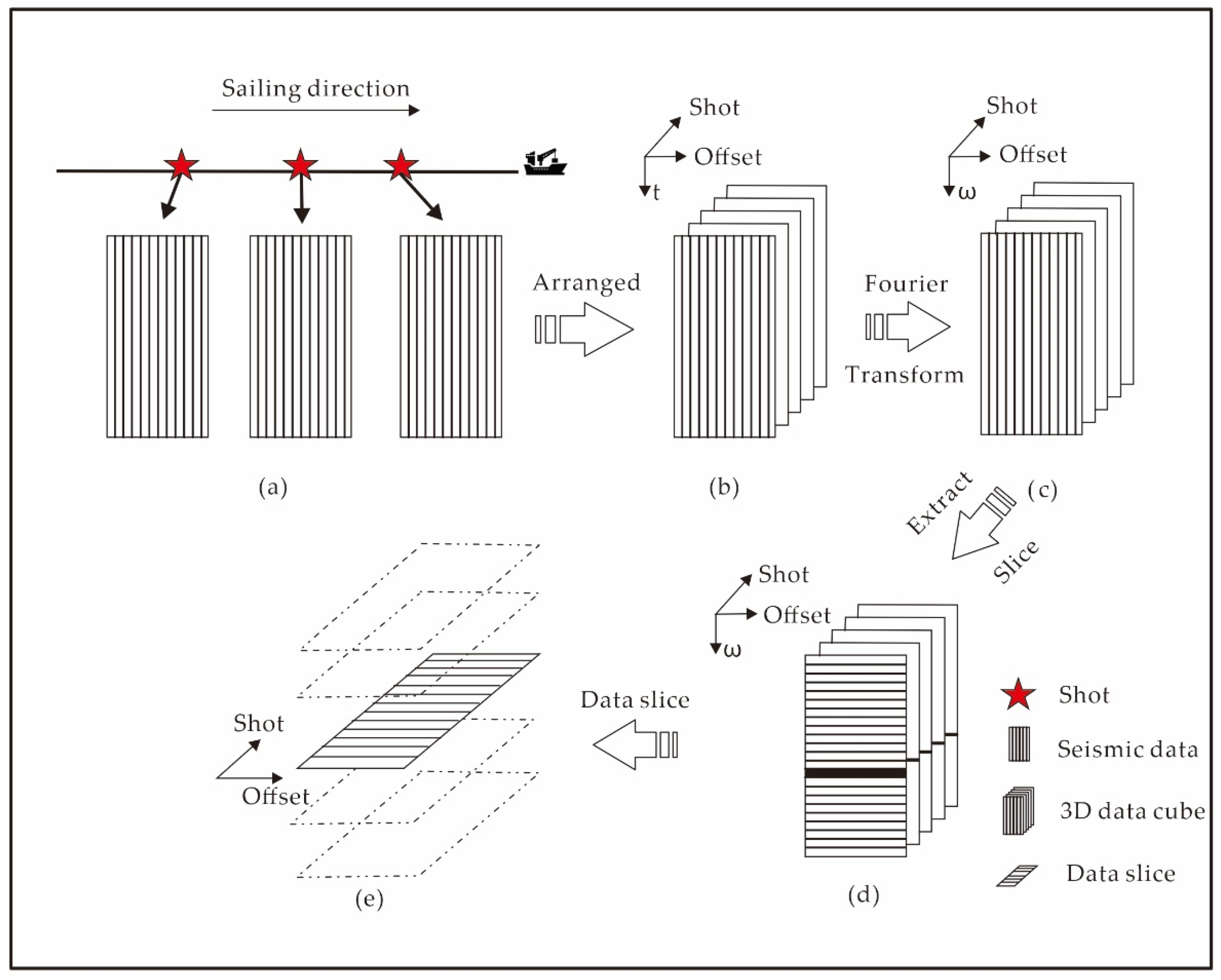
2.2.2. Multi-Shots’ Simultaneous Deghosting Framework

The signal of seismic data appears in different forms across different gathers. In common shot gathers, it is represented as high-curvature hyperbolas, while in common-offset gathers, it resembles the layers (smooth and continuous, which are suitable for nuclear norm constraints). Based on this feature, we designed a data preprocessing procedure that transforms 2D shot-by-shot arranged data into a 3D pseudo-data cube, providing more suitable input data for joint constraints’ inversion. With the modified data cube, we can achieve multi-shot simultaneous inversion, which improves efficiency while meeting the requirements of both regularization methods for the data.

For original data, in a conventional streamer observation system, the positions of the source and receivers are relatively fixed, which means that the offsets of different shots are consistent. Therefore, for the streamer data, we can simply rearrange the data from different shots (as shown in Figure 3) into a 3D data cube. This process can be simply understood as follows: Firstly, as shown in Figure 3a,b, the original data, which are shown in common shot gathers, are arranged according to shot numbers to obtain a 3D data cube. Then, by performing a Fourier transform along the time axis, we can obtain the frequency domain representation of the 3D data cube (as shown in Figure 3c). At this point, extracting it at any frequency slice will give us a 2D slice where the first dimension represents the shot number, and the second dimension represents the offset (as shown in Figure 3d,e).

However, for virtual data generated through seismic interferometry, it is not a cable system, but rather similar to conventional seismic acquisition systems; that is, the receiver remains stationary with the source moves, and the offsets between different shots are different. It means that if we rearrange the data as shown in Figure 3, the data slice along shots is not the common-offset gather, which is required by the nuclear norm constraint. Therefore, before constructing a pseudo-3D data cube, it is necessary to preprocess the virtual-shot data to form a common-offset gather. It is interesting that through the observation and analysis of virtual data, we found that with only a slight adjustment of the observation perspective, we can still easily obtain the desired common-offset gathers from the rearranged 3D data cube. The process is shown in Figure 4, and we present it in the form of a 3D data overview diagram.

For the virtual-shot gather, we can understand it as shown in Figure 4a. The receiver position of the acquisition system remains unchanged, the source position moves, and each receiver position undergoes an excitation. First, we rotate the data cube to Figure 4b and connect the data with the same offset in the red line. Then, with the shaded area being a zero matrix, as shown in Figure 4c, we can obtain the preprocessing result, in which the vertical slice of the 3D data cube becomes a common-offset gather (each vertical slice is connected by red lines). The frequency domain slices of the data can be represented as

$$D_{\mathrm{pse}\text{-}3\mathrm{D}}({\omega }_k)=\left[\begin{array}{ccccc}{D}_1^v(x_{-ntr},{\omega }_k)& \cdot \cdot \cdot & D_1^v(x_j,{\omega }_k)& \cdot \cdot \cdot & D_1^v(x_{ntr},{\omega }_k)\\ \cdot \cdot \cdot & \cdot \cdot \cdot & \cdot \cdot \cdot & \cdot \cdot \cdot & \cdot \cdot \cdot \\ D_i^v(x_{-ntr},{\omega }_k)& \cdot \cdot \cdot & D_i^v(x_j,{\omega }_k)& \cdot \cdot \cdot & D_i^v(x_{ntr},{\omega }_k)\\ \cdot \cdot \cdot & \cdot \cdot \cdot & \cdot \cdot \cdot & \cdot \cdot \cdot & \cdot \cdot \cdot \\ D_{ns}^v(x_{-ntr},{\omega }_k)& \cdot \cdot \cdot & D_{ns}^v(x_j,{\omega }_k)& \cdot \cdot \cdot & D_{ns}^v(x_{ntr},{\omega }_k)\end{array}\right],$$

(14)

where $ns$ is the number of shots, and $ntr$ represents the number of traces and

$$D_i^v(x_j,\omega )=\left\{\begin{array}{cc}0& \begin{array}{cc}& x_{-ntr}<x_j<x_{-i}\end{array}\\ D_{i-(j+1)/2}(x_{i+(j-1)/2},\omega )& \begin{array}{cc}& x_{-i}\le x_j\le x_i\end{array}\\ 0& \begin{array}{cc}& x_i<x_j<x_{ntr}\end{array}\end{array}\right.,$$

(15)

among them; $s_i$ represents the $i_{th}$ shot, $x_i$ is the offset coordinate, and its value range is $-x_{ntr}\le x_j\le x_{ntr}$. In this way, we can rearrange the virtual-shot data into a pseudo-3D data cube.

Through the aforementioned data preprocessing steps, we obtain the input data $D_{\mathrm{pse}\text{-}3\mathrm{D}}$ that meet the requirements of the joint constraint inversion. Then, we can derive the objective function of the inversion framework:

$$F(S_{\mathrm{pse}\text{-}3\mathrm{D}})={‖G{S}_{\mathrm{pse}\text{-}3\mathrm{D}}-D_{\mathrm{pse}\text{-}3\mathrm{D}}‖}_F^2+\lambda {‖S_{\mathrm{pse}\text{-}3\mathrm{D}}‖}_1+\mu {‖S_{\mathrm{pse}\text{-}3\mathrm{D}}‖}_{\ast }.$$

(16)

Equation (16) can be solved using a split Bergman iteration strategy and introducing auxiliary variable matrix $\Theta$. Equation (16) can be rewritten as

$$F(S_{\mathrm{pse}\text{-}3\mathrm{D}},\Theta )={‖G{S}_{\mathrm{pse}\text{-}3\mathrm{D}}-D_{\mathrm{pse}\text{-}3\mathrm{D}}‖}_F^2+\lambda {‖\Theta ‖}_1+\beta {‖S_{\mathrm{pse}\text{-}3\mathrm{D}}-\Theta ‖}_F^2+\mu {‖S_{\mathrm{pse}\text{-}3\mathrm{D}}‖}_{\ast },$$

(17)

and among them, $\beta$ is an auxiliary parameter in the split Bergman iteration. Equation (17) can be iteratively solved by alternately minimizing the $\Theta$ and $S_{\mathrm{pse}\text{-}3\mathrm{D}}$.

Firstly, we will introduce how to minimize the auxiliary matrix $\Theta$. $\Theta$ can be obtained by solving the objective function shown in Equation (18):

$$F({\Theta }^k)=\beta {‖S_{\mathrm{pse}\text{-}3\mathrm{D}}^{k-1}-{\Theta }^k‖}_F^2+\lambda {‖{\Theta }^k‖}_1,$$

(18)

where $k$ is the number of iterations. This function can be solved through the threshold shrinkage algorithm [41]:

$${\Theta }^k=T_t(S_{\mathrm{pse}\text{-}3\mathrm{D}}^{k-1}),$$

(19)

where $t=\frac{\lambda }{2\beta }$, and $T_t(S_{\mathrm{pse}\text{-}3\mathrm{D}}^{k-1})$ is the threshold shrinkage operator:

$$T_t(S_{\mathrm{pse}\text{-}3\mathrm{D}})=\left\{\begin{array}{cc}{S}_{i,j}-t& S_{i,j}\ge t>0\\ 0& -t<S_{i,j}<t\\ S_{i,j}+t& S_{i,j}<-t\end{array}\right.,$$

(20)

where $S_{\mathrm{pse}\text{-}3\mathrm{D}}$ can be obtained by solving the objective function of Equation (21), which requires the use of auxiliary matrices $\Theta$.

$$F(S_{\mathrm{pse}\text{-}3\mathrm{D}}^k)={‖G{S}_{\mathrm{pse}\text{-}3\mathrm{D}}^k-D_{\mathrm{pse}\text{-}3\mathrm{D}}‖}_F^2+{\beta }^{k-1}{‖S_{\mathrm{pse}\text{-}3\mathrm{D}}^k-{\Theta }^k‖}_F^2+\mu {‖S_{\mathrm{pse}\text{-}3\mathrm{D}}^k‖}_{\ast },$$

(21)

which can be rewritten as

$$F(S_{\mathrm{pse}\text{-}3\mathrm{D}}^k)={‖A-L{S}_{\mathrm{pse}\text{-}3\mathrm{D}}^k‖}_F^2+\mu {‖S_{\mathrm{pse}\text{-}3\mathrm{D}}^k‖}_{\ast },$$

(22)

where $A=\left[\begin{array}{c}{D}_{\mathrm{pse}\text{-}3\mathrm{D}}\\ \sqrt{\beta }{\Theta }^k\end{array}\right]$ and $L=\left[\begin{array}{c}G\\ \sqrt{\beta }I\end{array}\right]$. Equation (22) can be solved by an approximate message passing algorithm [42].

In summary, Equation (16) can be solved by the following steps:

Step 1: Input data contain ghost $D_{\mathrm{pse}\text{-}3\mathrm{D}}$, ghost operator $G$, zero matrix $S^0$, regularization parameters $\lambda$ and $\mu$, and auxiliary parameters ${\beta }^0$. Set $k=1$.

Step 2: Obtain the auxiliary matrix ${\Theta }^k$ through Equation (20).

Step 3: Substituting ${\Theta }^k$ into Equation (21) to obtain the matrix $S^k$.

Step 4: Determine if $S^k$ meets the requirement $\frac{{‖S^k-S^{k-1}‖}_F^2}{1+{‖S^k‖}_F^2}<\epsilon$, where $\epsilon$ is the Bregman iteration stop parameter, or if the desired number of iterations has been reached. If so, stop the iteration. If not, set $k=k+1$ and ${\beta }^k=a{\beta }^{k-1},a\in (1,2)$ and return to Step 2.

2.3. Data Description

The performance of the proposed multi-shot simultaneous deghosting method in this article is evaluated on three datasets: the passive seismic synthetic data, the active seismic synthetic data, and field data. Details of all datasets are described as follows:

2.3.1. Synthetic Data

The velocity model used is the salt dome model (Figure 5). This model has 250 grid points in the vertical direction and 1081 sampling points in the horizontal direction, with a grid spacing of 5 m. The model includes various velocity layers and contains a large number of geological anomalies. These complex geological structures (including high-velocity layers and faults) and significant velocity variations result in a highly complex synthetic seismic wavefield. This complexity effectively tests the method’s efficacy in handling intricate situations, making it widely used in seismic exploration-related research [1,2]. In this study, we applied this model to generate synthetic datasets and test the effectiveness of the multi-shot simultaneous deghosting method.

First, we use synthetic datasets to test the effectiveness of the multi-shot simultaneous deghosting method (the detailed acquisition system parameter settings are provided in

Table 1. Parameter setting of Synthetic data.

Acquisition System	Parameter Setting
Source	271
Receivers	271
Trace spacing	20 m
Shot spacing	20 m
Time sampling	2 ms
Total time	1.6 s
Receiver depth	20 m

). Recognizing the applicability of both active and passive seismic data in constructing virtual-shot gathers via seismic interferometry, we conducted separate analyses on these datasets (Figure 6).

We used the finite difference seismic forward modeling method and Ricker wavelet with a main frequency of 30 Hz to generate the synthetic data. Among them, Figure 6a,b are the virtual-shot gathers obtained by passive and active seismic data, respectively. The air–water surface was set as a free surface. Additionally, the sides of the model were configured with absorbing boundaries to prevent unnecessary interfering wavefields.

2.3.2. Field Data

Field data were collected (Figure 7) in the South Sea of China using a steamer system. In

Table 2. Parameter setting of Field data.

Acquisition System	Parameter Setting
Source	371
Receivers	371
Trace spacing	25 m
Shot spacing	25 m
Time sampling	4 ms
Total time	2.4 s
Receiver depth	7 m

, we provide the relevant information for this field data. These data were acquired using a steamer observation system, which is a unique marine exploration system that involves towing a series of receivers behind a survey vessel to continuously collect seismic data along predefined lines. During the acquisition process, the source points and receivers move with the survey vessel, resulting in the obtained data having a fixed offset in different shot gathers. Compared to the synthetic data, the layers are relatively gentle, but the wavefield is more complex, which is a challenge to the stability of the deghosting method.

3. Results

In this section, the original data (contain ghosts) and the result of the widely used Radon-based deghosting method will be used as the control group. Because of the effect of the ghost shown in both the data domain and frequency domain, in each test, we will provide the data domain deghosting results and frequency domain result (f-k spectra). In this section, we will compare the kinematic characteristics and frequency bands of different methods on seismic records, which aims to comprehensively verify the effectiveness of the proposed multi-shot simultaneous deghosting framework.

3.1. Synthetic Data Result

First, we use the passive synthetic data to test the effectiveness of the multi-shot simultaneous deghosting method. The data domain deghosting results are shown in Figure 8. Through Figure 8, we mainly compare the impact of different deghosting methods on kinematic characteristics of the seismic events. Firstly, from an overall perspective, comparing the original data shown in Figure 8a, both the conventional deghosting method and the multi-shot simultaneous deghosting framework reduced the impact of the ghost. This phenomenon is mainly shown in the two events of 0.3 s and 0.5 s in the slice of a common shot gather. In the original data (Figure 8a), the events shown in black are followed by the events with opposite polarity (shown in white), which is due to the delay superposition between the ghost and the original data, but in Figure 8b,c, the negative polarity events disappear. When we compare the processing effects shown in Figure 8b,c, we can find that there is a significant difference between the two methods. At the position indicated by the yellow arrow in a common shot gather near 0.4 s, due to the strong energy at the near offset, the conventional deghosting method exhibits instability, and non-physical events appear in seismic records. But, in Figure 8c, this phenomenon does not occur, which proved the effectiveness of the multi-shot simultaneous deghosting method. Similarly, we can observe that regarding the common-offset gather, the results obtained by the multi-shot simultaneous deghosting method are also more accurate than those obtained by the conventional method. It can be observed that the conventional method also leads to the presence of non-physical events due to inversion instability. In the meantime, marked by a yellow arrow, the layer present in the original data is almost masked by the introduced noise in Figure 8b, but in the multi-shot simultaneous deghosting method, the layer can still be clearly observed. This proves the superiority of the multi-shot simultaneous deghosting method over conventional methods.

By applying the Fast Fourier Transform (FFT) to the time-domain data shown in Figure 8, we can obtain the f-k spectra for the three datasets (shown in Figure 9) to further validate the effectiveness through the aspect of frequency band compensation. The impact of the ghost on the data frequency band is mainly reflected in two aspects; one is the absence of low frequency, and the other is the generation of notch frequencies. In the passive virtual-shot gathers, the latter is the main phenomenon of ghost impact. The theoretical notch frequency due to ghosting can be calculated using the equation $f_n=n\frac{c}{2z},n=0,1,2,\cdots$, where $z$ is receiver depth, and $c$ is water velocity. Substituting the water velocity and the receiver depth, we can obtain that the notch frequency should be concentrated near 37.5 Hz. To better compare the compensation effects of different methods on this notch frequency, we selected the frequency band range of the f-k spectrum to be 0–50 Hz. From Figure 9a, it can be observed that the notch frequency is near the 35 Hz position (marked by red arrows). In Figure 9b,c, both results compensate for the notch effect. However, it is evident that there is an obvious outlier in the processing results of the conventional method shown in Figure 9b, which is caused by the instability of the inversion algorithm. But, in the multi-shot simultaneous deghosting framework shown in Figure 9c, results have the complete frequency band without outliers. Through this comparative experiment, we have verified that the multi-shot simultaneous deghosting framework can achieve better processing results than conventional methods in passive virtual-shot gathers. Whether from the kinematic characteristics of the events shown in the data domain or frequency band shown in the f-k spectrum, it has been proven that the multi-shot simultaneous deghosting framework has strong stability, which can avoid interference caused by inversion instability.

Similar to the passive seismic data, we compare the effects of different deghosting methods on the kinematic characteristics of events in the data domain (Figure 10) and frequency band compensation (Figure 11). By comparing the original data (Figure 10a), conventional deghosting result (Figure 10b), and multi-shot simultaneous deghosting result (Figure 10c), we can clearly see changes in the polarity of seismic events after deghosting. At the position marked by the red arrow, the negative polarity (white) seen in Figure 10a, caused by the delay superposition of the ghost and the original data, is suppressed in Figure 10b,c, indicating the effectiveness of the deghosting method. Comparing the results shown in Figure 10b,c, it can be seen that due to the improvement in inversion stability, the interference introduced by the conventional deghosting method (marked by yellow arrow) does not appear in Figure 10c. Whether in the time slice or the common-offset slice, the processing results of the multi-shot simultaneous deghosting framework are better than those of the conventional method, specifically shown in better event continuity and the disappearance of false layers.

In the f-k spectrum of the original data shown in Figure 11a, it can be observed that due to the influence of the ghost, there is low frequency missing at the 0–10 Hz position, and a notch phenomenon near 40 Hz. Firstly, we compare the compensation effects of two deghosting methods for missing low frequency. In Figure 11b,c, we can see that the missing low-frequency wavefield in both results is compensated, but the result of the multi-shot simultaneous deghosting method has stronger energy, which will bring convenience for subsequent processing. For the frequency band notch near 40 Hz, it can be seen that after notch compensation, the frequency band continuity of the multi-shot simultaneous deghosting method is significantly better than the processing results of conventional methods because of the outliers caused by inversion instability. The processing results in the f-k spectrum fully demonstrate that the multi-shot simultaneous deghosting framework can achieve better processing results than conventional methods in the active source virtual data, demonstrating the effectiveness of the multi-shot simultaneous deghosting framework.

3.2. Field Data Result

Furthermore, we used the field data to test the effectiveness of the multi-shot simultaneous deghosting framework. The result is shown in Figure 12. In Figure 12, to better present the results, we adjusted the display range of the offset, mainly focusing on the near-offset data that contains more information. Overall, both conventional deghosting methods and the multi-shot simultaneous deghosting framework have successfully suppressed the ghost in the original data, as shown by the red arrow in the time slice. The seismic wave field formed by the delay superposition of the ghost and the original data (shown in white) is suppressed in Figure 12b,c. By comparing the processing results of the two methods in detail, we can find that the conventional method, due to the instability of the inversion process, not only attenuates the ghost but also affects the effective signal. At the position indicated by the yellow arrow in the shot slice, it can be seen that the results processed by the conventional method show waveform distortion compared to the original data and the results processed by the multi-shot simultaneous deghosting method. Meanwhile, there is a phenomenon of real strata being masked in the common-offset slice. For a more intuitive comparison, in Figure 13, we present the zoom view of the position marked by the red dotted box in the common-offset slice of Figure 12.

By comparing Figure 13, we observe that the multi-shot simultaneous deghosting framework (Figure 13c) provides better continuity and higher resolution than the conventional method (Figure 13b), and shows a certain noise suppression effect. At the positions marked by yellow arrows, we can see that Figure 13b, compared to Figure 13c, lacks some data. This indicates that the conventional method has caused damage to the effective signal due to instability in the inversion process. However, the multi-shot simultaneous deghosting framework (Figure 13c) effectively protects the signals. The analysis of data domain processing results shows that the multi-shot simultaneous deghosting framework achieves better results in field data, balancing deghosting and signal protection, thereby proving its effectiveness.

In Figure 14, we present the f-k spectrum of field data and evaluate the compensation effect of the method for missing frequency bands through a frequency band analysis. Compared to the original data (Figure 14a), the results in Figure 14b,c both enhance low-frequency signals within 10 Hz. However, the multi-shot simultaneous deghosting framework provides better energy compensation, resulting in stronger frequency band energy than the conventional method. This demonstrates the frequency band compensation capability of the multi-shot simultaneous deghosting framework in processing field data.

4. Conclusions

This study demonstrates an innovative approach to multi-shot simultaneous ghosting by integrating sparse and nuclear norm-constrained inversion. Our method focuses on constructing a pseudo-3D data cube and introducing joint sparsity and nuclear norm-constrained inversion, significantly enhancing ghost separation accuracy. The new method effectively balances computational demands and inversion accuracy. Synthetic and field examples show significant improvement in accuracy and stability with the multi-shot simultaneous deghosting method. The practical application of seismic interferometry marks a major advance in the field and offers a promising direction for future seismic data processing and interpretation.

References

1. Snieder, R.; Miyazawa, M.; Slob, E.; Vasconcelos, I.; Wapenaar, K. A Comparison of Strategies for Seismic Interferometry. Surv. Geophys. 2009, 30, 503–523. [Google Scholar] [CrossRef]
2. Wang, X.; Zhang, J.; Guo, C.; Zhao, S.; Cheng, H. Seismic Interferometry in Linear Radon Domain Applying to Noise Passive Data. IEEE Geosci. Remote Sens. Lett. 2022, 19, 1–5. [Google Scholar] [CrossRef]
3. Ramirez, A.C.; Weglein, A.B.; Otnes, E.; Hokstad, K. The role of the direct wave and Green’s theorem in seismic interferometry and spurious multiples. In SEG Technical Program Expanded Abstracts 2007; Society of Exploration Geophysicists: Houston, TX, USA, 2007; pp. 2471–2475. [Google Scholar]
4. Wang, Y.; Luo, Y.; Schuster, G.T. Interferometric interpolation of missing seismic data. Geophysics 2009, 74, SI37–SI45. [Google Scholar] [CrossRef]
5. Melo, G.; Malcolm, A.; Fehler, M. Comparison of microearthquake locations using seismic interferometry principles. In SEG Technical Program Expanded Abstracts 2012; Society of Exploration Geophysicists: Houston, TX, USA, 2012; pp. 1–5. [Google Scholar]
6. Gu, N.; Chamarczuk, M.; Gao, J.; Malinowski, M.; Zhang, H. Passive seismic structure imaging of a coal mine by ambient noise seismic interferometry on a dense array. Acta Geol. Sin. Engl. Ed. 2021, 95, 37–39. [Google Scholar] [CrossRef]
7. Yu, J.; Kim, B.-Y.; Joo, Y. A processing for ocean-bottom multicomponent data with seismic interferometry: A case study of southern offshore in Korea. Explor. Geophys. 2023, 54, 533–543. [Google Scholar] [CrossRef]
8. Zhang, F.; Zhang, P.; Xu, Z.; Gong, X.; Han, L. Multisource Seismic Full Waveform Inversion of Metal Ore Bodies. Minerals 2022, 12, 4. [Google Scholar] [CrossRef]
9. Liu, Q.; Feng, X.; Liu, C.; Zhang, M.; Tian, Y.; Hou, H. Metallic mineral exploration by using ambient noise tomography in Ashele copper mine, Xinjiang, China. Geophysics 2022, 87, B221–B231. [Google Scholar] [CrossRef]
10. Curtis, A.; Nicolson, H.; Halliday, D.; Trampert, J.; Baptie, B. Virtual seismometers in the subsurface of the Earth from seismic interferometry. Nat. Geosci. 2009, 2, 700–704. [Google Scholar] [CrossRef]
11. Brenguier, F.; Baue, P.; Ben-Zion, Y.; Vernon, F.; Johnson, C.W.; Mordret, A.; Coutant, O.; Share, P.E.; Beauce, E.; Hollis, D.; et al. Train Traffic as a Powerful Noise Source for Monitoring Active Faults With Seismic Interferometry. Geophys. Res. Lett. 2019, 46, 9529–9536. [Google Scholar] [CrossRef]
12. Mao, S.; Lecointre, A.; van der Hilst, R.D.; Campillo, M. Space-time monitoring of groundwater fluctuations with passive seismic interferometry. Nat. Commun. 2022, 13, 4643. [Google Scholar] [CrossRef]
13. King, S.; Curtis, A. Suppressing nonphysical reflections in Green’s function estimates using source-receiver interferometry. Geophysics 2012, 77, Q15–Q25. [Google Scholar] [CrossRef]
14. Viens, L.; Van Houtte, C. Denoising ambient seismic field correlation functions with convolutional autoencoders. Geophys. J. Int. 2020, 220, 1521–1535. [Google Scholar] [CrossRef]
15. Hu, B.; Wang, D.; Wang, R. An Iterative Focal Denoising Strategy for Passive Seismic Data. Pure Appl. Geophys. 2020, 177, 4607–4622. [Google Scholar] [CrossRef]
16. Othman, A.; Iqbal, N.; Hanafy, S.M.; Bin Waheed, U. Automated Event Detection and Denoising Method for Passive Seismic Data Using Residual Deep Convolutional Neural Networks. IEEE Trans. Geosci. Remote Sens. 2022, 60, 1–11. [Google Scholar] [CrossRef]
17. van Groenestijn, G.J.A.; Verschuur, D.J. Estimation of primaries by sparse inversion from passive seismic data. Geophysics 2010, 75, SA61–SA69. [Google Scholar] [CrossRef]
18. Cheng, H.; Wang, D.-L.; Feng, F.; Zhu, H. Estimating primaries from passive seismic data. Explor. Geophys. 2015, 46, 184–191. [Google Scholar] [CrossRef]
19. Zhao, B.; Han, L.; Zhang, P.; Yin, Y. Weak Signal Enhancement for Passive Seismic Data Reconstruction Based on Deep Learning. Remote Sens. 2022, 14, 5318. [Google Scholar] [CrossRef]
20. Wei, J.; Liu, H.; Xing, L.; Du, D. Application of seismic interferometric migration for shallow seismic high precision data processing: A case study in the Shenhu area. J. Ocean Univ. China 2018, 17, 46–52. [Google Scholar] [CrossRef]
21. Ghosh, S.K. Deconvolving the ghost effect of the water surface in marine seismics. Geophysics 2000, 65, 1831–1836. [Google Scholar] [CrossRef]
22. Amundsen, L.; Weglein, A.B.; Reitan, A. On seismic deghosting using integral representation for the wave equation: Use of Green’s functions with Neumann or Dirichlet boundary conditions. Geophysics 2013, 78, T89–T98. [Google Scholar] [CrossRef]
23. Seher, T.; Ren, Y.; Masoomzadeh, H.; Degel, T.; Cho, E.; Hawke, M.; Baldock, S. Deconvolution of upgoing and downgoing wavefields: A data example from the Utsira OBN survey. In Proceedings of the 83rd EAGE Annual Conference & Exhibition, Madrid, Spain, 6–9 June 2022; pp. 1–5. [Google Scholar]
24. Wang, P.; Ray, S.; Nimsaila, K. 3D joint deghosting and crossline interpolation for marine single-component streamer data. In Proceedings of the SEG International Exposition and Annual Meeting, Denver, CO, USA, 26–31 October 2014; p. SEG-2014-0882. [Google Scholar]
25. King, S.; Poole, G. Hydrophone-only receiver deghosting using a variable sea surface datum. In Proceedings of the SEG International Exposition and Annual Meeting, New Orleans, Louisiana, 18–23 October 2015; p. SEG-2015-5891123. [Google Scholar]
26. Zhang, Z.; Masoomzadeh, H.; Wang, B. Evolution of deghosting process for single-sensor streamer data from 2D to 3D. Geophys. Prospect. 2018, 66, 975–986. [Google Scholar] [CrossRef]
27. Cao, J.; Blacquière, G. Receiver Deghosting with Blended Data Using Sparse Inversion. In Proceedings of the 82nd EAGE Annual Conference & Exhibition, Amsterdam, The Netherlands, 18–21 October 2021; pp. 1–5. [Google Scholar]
28. Hardwick, A.; Charron, P.; Masoomzadeh, H.; Aiyepeku, A.; Cox, P.; Laha, S. Accounting for sea surface variation in deghosting–a novel approach applied to a 3D dataset offshore west Africa. In SEG Technical Program Expanded Abstracts 2015; Society of Exploration Geophysicists: Houston, TX, USA, 2015; pp. 4615–4619. [Google Scholar]
29. Vrolijk, J.-W.; Blacquiere, G. Source deghosting of coarsely sampled common-receiver data using a convolutional neural network. Geophysics 2021, 86, V185–V196. [Google Scholar] [CrossRef]
30. de Jonge, T.; Vinje, V.; Poole, G.; Zhao, P.; Iversen, E. Deghosting dual-component streamer data using demigration-based supervised learning. Geophys. Prospect. 2023, 72, 68–91. [Google Scholar] [CrossRef]
31. Almuteri, K.; Sava, P. A convolutional neural network approach for ghost removal. In Proceedings of the SEG International Exposition and Annual Meeting, Denver, CO, USA, 26 September–1 October 2021; p. D011S110R001. [Google Scholar]
32. Poole, G. Pre-migration receiver de-ghosting and re-datuming for variable depth streamer data. In Proceedings of the SEG International Exposition and Annual Meeting, Houston, TX, USA, 22–27 September 2013; p. SEG-2013-0541. [Google Scholar]
33. Curtis, A.; Gerstoft, P.; Sato, H.; Snieder, R.; Wapenaar, K. Seismic interferometry—Turning noise into signal. Lead. Edge 2006, 25, 1082–1092. [Google Scholar] [CrossRef]
34. Liu, L.; Liu, Y.; Li, T.; He, Y.; Du, Y.; Luo, Y. Inversion of vehicle-induced signals based on seismic interferometry and recurrent neural networks. Geophysics 2021, 86, Q37–Q45. [Google Scholar] [CrossRef]
35. Bleistein, N. Mathematical Methods for Wave Phenomena; Academic Press: Cambridge, MA, USA, 2012. [Google Scholar]
36. Nie, W.; Xiang, F.; Li, B.; Wen, X.; Nie, X. Prestack Seismic Inversion via Nonconvex L1-2 Regularization. Appl. Sci. 2021, 11, 12015. [Google Scholar] [CrossRef]
37. Liu, L.; Ma, J.; Plonka, G. Sparse graph-regularized dictionary learning for suppressing random seismic noise. Geophysics 2018, 83, V215–V231. [Google Scholar] [CrossRef]
38. Hamid, H.; Pidlisecky, A. Multitrace impedance inversion with lateral constraints. Geophysics 2015, 80, M101–M111. [Google Scholar] [CrossRef]
39. Shao, O.; Wang, L.; Hu, X.; Long, Z. Seismic denoising via truncated nuclear norm minimization. Geophysics 2021, 86, V153–V169. [Google Scholar] [CrossRef]
40. Zhang, W.; Fu, L.; Zhang, M.; Cheng, W. 2-D seismic data reconstruction via truncated nuclear norm regularization. IEEE Trans. Geosci. Remote Sens. 2020, 58, 6336–6343. [Google Scholar] [CrossRef]
41. Elad, M. Sparse and Redundant Representations: From Theory to Applications in Signal and Image Processing; Springer: Berlin/Heidelberg, Germany, 2010; Volume 2. [Google Scholar]
42. Donoho, D.L.; Maleki, A.; Montanari, A. Message-passing algorithms for compressed sensing. Proc. Natl. Acad. Sci. USA 2009, 106, 18914–18919. [Google Scholar] [CrossRef] [PubMed]
43. Davis, G.; Mallat, S.; Avellaneda, M. Adaptive greedy approximations. Constr. Approx. 1997, 13, 57–98. [Google Scholar] [CrossRef]
Figure 1. A demonstration of seismic data before and after seismic interferometry: (a) Original data. (b) The corresponding virtual-shot gather.
Remotesensing 16 02075 g001
Figure 2. A demonstration of different source data. (a) Active seismic data. (b) Passive seismic data.
Remotesensing 16 02075 g002
Figure 3. Data rearrangement schematic: (a) The acquired original data (shown in common shot gathers). (b) The pseudo-3D data cube which obtained by arranging the original data by shot number. (c) Frequency-domain pseudo-3D data cube. (d) Extract frequency slices from the frequency-domain data cube. (e) The extracted frequency slices.
Remotesensing 16 02075 g003
Figure 4. Schematic diagram of virtual-shot data rearrangement. (a) Top view of the 3D data cube where we illustrate the relative positions of the sources and receivers. (b) Top view of the rotated pseudo-3D data cube, where the red lines indicate data with the same offset. (c) Top view of the preprocessed results, with shaded areas indicating filled zero matrices.
Remotesensing 16 02075 g004
Figure 5. Salt dome velocity model.
Remotesensing 16 02075 g005
Figure 6. The 3D data cube of original synthetic data: (a) Virtual-shot gathers of passive seismic data. (b) Virtual-shot gathers of active seismic data. The blue lines indicate the positions of the displayed slices within the data cube, that is, the three slices shown from the 3D cube are: a time slice at 0.8 s, a common shot gather at shot number 135, and a common offset gather at an offset of 0 km.
Remotesensing 16 02075 g006
Figure 7. The 3D data cube of original field data. The blue lines indicate the positions of the displayed slices within the data cube.
Remotesensing 16 02075 g007
Figure 8. The data domain deghosting result of passive seismic data: (a) The input data which contain ghosts. (b) Radon-based inversion deghosting result. (c) Multi-shot simultaneous deghosting result. The locations of noise introduced are marked by yellow arrows. The blue lines indicate the positions of the displayed slices within the data cube.
Remotesensing 16 02075 g008aRemotesensing 16 02075 g008b
Figure 9. The frequency domain deghosting result of passive seismic data: (a) The input data which contain ghosts. (b) Radon-based inversion deghosting result. (c) Multi-shot simultaneous deghosting result. The locations of frequence notch compensation are marked by red arrows.
Remotesensing 16 02075 g009
Figure 10. The data domain deghosting result of active seismic data: (a) The input data which contain ghosts. (b) Radon-based inversion deghosting result. (c) Multi-shot simultaneous deghosting result. The locations of the denoising effect are marked by red arrows, and the location of noise introduced is marked by a yellow arrow. The blue lines indicate the positions of the displayed slices within the data cube.
Remotesensing 16 02075 g010aRemotesensing 16 02075 g010b
Figure 11. The frequency domain deghosting result of active seismic data: (a) The input data which contain ghosts. (b) Radon-based inversion deghosting result. (c) Multi-shot simultaneous deghosting result.
Remotesensing 16 02075 g011
Figure 12. The data domain deghosting result of field data: (a) The input data which contain ghosts. (b) Radon-based inversion deghosting result. (c) Multi-shot simultaneous deghosting result. The locations of the denoising effect are marked by red arrows, and the location of waveform distortion is marked by yellow arrows. The red dotted box marks the position needed to provide a zoom view. The blue lines indicate the positions of the displayed slices within the data cube.
Remotesensing 16 02075 g012aRemotesensing 16 02075 g012b
Figure 13. Zoom views of the position marked by a red dotted box of the data domain deghosting result of field data: (a) The input data which contain ghosts. (b) Radon-based inversion deghosting result. (c) Multi-shot simultaneous deghosting result. The location of the damaged signal is marked by yellow arrows.
Remotesensing 16 02075 g013
Figure 14. The frequency domain deghosting result of the field data: (a) The input data which contain ghosts. (b) Radon-based inversion deghosting result. (c) Multi-shot simultaneous deghosting result.
Remotesensing 16 02075 g014