Article

Identifying Plausible Labels from Noisy Training Data for a Land Use and Land Cover Classification Application in Amazônia Legal

by
Maximilian Hell
* and
Melanie Brandmeier
Faculty of Plastics Engineering and Surveying, Technical University of Applied Sciences Würzburg-Schweinfurt (THWS), 97070 Würzburg, Germany
*
Author to whom correspondence should be addressed.
Remote Sens. 2024, 16(12), 2080; https://doi.org/10.3390/rs16122080
Submission received: 5 April 2024 / Revised: 28 May 2024 / Accepted: 6 June 2024 / Published: 8 June 2024
(This article belongs to the Section AI Remote Sensing)

Abstract

:
Most studies in the field of land use and land cover (LULC) classification in remote sensing rely on supervised classification, which requires a substantial amount of accurate label data. However, reliable data are often not immediately available, and are obtained through time-consuming manual labor. One potential solution to this problem is the use of already available classification maps, which may not be the true ground truth and may contain noise from multiple possible sources. This is also true for the classification maps of the MapBiomas project, which provides land use and land cover (LULC) maps on a yearly basis, classifying the Amazon basin into more than 24 classes based on the Landsat data. In this study, we utilize the Sentinel-2 data with a higher spatial resolution in conjunction with the MapBiomas maps to evaluate a proposed noise removal method and to improve classification results. We introduce a novel noise detection method that relies on identifying anchor points in feature space through clustering with self-organizing maps (SOM). The pixel label is relabeled using nearest neighbor rules, or can be removed if it is unknown. A challenge in this approach is the quantification of noise in such a real-world dataset. To overcome this problem, highly reliable validation sets were manually created for quantitative performance assessment. The results demonstrate a significant increase in overall accuracy compared to MapBiomas labels, from 79.85% to 89.65%. Additionally, we trained the L2HNet using both MapBiomas labels and the filtered labels from our approach. The overall accuracy for this model reached 93.75% with the filtered labels, compared to the baseline of 74.31%. This highlights the significance of noise detection and filtering in remote sensing, and emphasizes the need for further research in this area.

1. Introduction

The Amazon Rainforest is one of the largest and most diverse ecosystems on earth, accommodating approximately one third of Earth’s species, a quarter of all freshwater, and houses indigenous communities [1]. Its trees absorb two billion tons of CO2 per annum from their surrounding atmosphere. In exchange, the forest generates 20% of Earth’s oxygen [2]. Despite its immeasurable value, this ecosystem is threatened by human deforestation, degradation, and massive land use and land cover changes. A complex chain of political and socio-economic decisions has lead to an increased deforestation rate in the Brazilian part of the rainforest [3,4]. The PRODES project monitors the clear-cutting of the Amazon Rainforest in Amazônia Legal and observed a steady rise in deforestation since 2012 [5]. They recorded a forest loss of 10,851 km2 in 2020 alone, which was then converted to other land use and cover forms. In the years from 1985 to 2017, approximately 38% of the land in Brazil was converted to pasture and farming usage, with an accompanied vegetation loss of 42.8% in the Amazon region [6]. Monitoring of this region is of utmost importance, as the occurring changes not only impact the local region, but also influence global climate [7]. Various projects and scientific research are concerned with the classification of the land surface in this area, to capture these events and assess their impact. One notable project is MapBiomas, a collaboration between various researchers, specialists, and NGOs. They produce annual complete land cover maps of Brazil with 30 m spatial resolution based on Landsat imagery time-series [6]. These maps can be used as baseline label data for training classifiers on data with a higher spatial and temporal resolution. The challenge of acquiring good training data and its related cost leads to one of the most prominent problems in supervised learning: the sparsity of good annotated data. Training data that is reliable and can act as a ground truth is often unavailable, and requires a lot of time from annotators to be created. The time to annotate data can be mitigated by using machine or deep learning classification models, which take a smaller amount of training data and extrapolate to other data or regions. This is performed by using already-prepared land use and land cover maps, such as MapBiomas, as ground truth data [8]. In the context of satellite remote sensing, this means only annotating few pixels or areas manually, and then training a classifier with these data to produce area-covering maps of land use and land cover. However, these models are also not certain in the classification, and misclassify samples which are outside of the learned distributions or uncertain in the separation between classes. Furthermore, the approach of using label data from other classifiers entails more challenges: classified labels can be incorrect (meaning wrong assigned class) or inaccurate (meaning the resolutions of label and training data are not the same) [9]. These types of wrong labels can be collectively termed as noisy labels, and learning with them is a weakly supervised task. Previous works have shown that noise in supervised training decreases the classification performance significantly [10]. Thus, it is important to develop training or filtering methods that are robust to noise, or even detects it. This, in turn, should lead to better performing and generalizing models, as the input to the models is cleaner and should mitigate memorization of wrong relationships between the data and the label. In this paper, we will present a novel approach for filtering and relabeling noisy labels from the MapBiomas project for later classification on higher resolution satellite data than the one used in the project. The proposed semi-supervised machine learning approach does not rely on a specific learned model, and rather only relies on the relationships between the input and label data. The classification improvement is then assessed using the L2HNet trained on the improved vs. original labels with accuracy assessment conducted using manually labeled validation data. Our novel approach can be termed model-independent and data-centric.

Learning with Noisy Labels

Supervised machine and deep learning methods mostly rely on clean training data to learn a good generalization of the underlying data distribution. However, real-life applications are often noisy in their input data, as well as in their labeled data. Label noise, also termed class noise in some of the literature [11], stems from multiple sources. It can occur through human mistakes or unclear differences between classes to a human interpreter [12,13]. With regard to remote sensing and land use and land cover (LULC) classification, the label noise can also be dependent on the time at which the label was identified. An example of this is in the agricultural sector, where fields might be fallow for some time and are planted during other times. They can also be planted with different crops at different points in time. The labels used in the presented study are derived from machine and deep learning models, cf. Section 2.1, which also inherently carry errors and biases. Further noise is introduced through the spatial mismatch of the label and input data. Both rasters do not overlap perfectly, and the spatial resolution are not the same. This is also known as inaccurate label data [9]. The existence of noisy labels within a training data set leads to a loss in detection performance [14], especially in conjunction with the memorization effect of highly parameterized models [15].
There are a multitude of approaches on how to handle or even identify noisy label data. This challenge has already been studied back in the 1960s [16], and is even more relevant today with multiple orders of magnitude more data available. The strategies for learning with label noise can be roughly grouped into data-centric and learning-centric methods [17,18,19]. In learning- or model-centric approaches, the methods depend on a supervised model to be learned. These methods are often concerned with robust learning and, thus, indirectly handle the noise. Early approaches learned an ensemble of models to then identify misclassified examples in multiple different classification models [13,20,21]. Other approaches make use of different loss functions during the training of the classification model to be more robust against noisy examples [22,23,24,25], correcting the loss during the learning process [26], or a joint optimization approach [27]. Also, ref. [28] presented an approach to use a k-NN filtering at the logit layer of a trained deep learning model to remove mislabeled data. Further methods rely on building noise transition matrices, which reflect the transition probability from one label to another, resulting in a noisy example [29]. Other works proposed special frameworks, which are purpose build to identify noise in the label data during the learning process and, in some instances, even correcting them at run-time [10,30,31,32]. Ref. [33] used negative learning, meaning labels that exclude impossible class labels, in conjunction with positive learning, to achieve robustness against noisy samples, whereas in data-centric methods, the focus on the relationship between the data and it is labels, i.e., outlier detection or clustering techniques, without the need to learn (semi-)supervised models in the process of it. Wilson et al. [34,35] presented algorithms that are noise-tolerant based on the k-nearest neighbors of training instances to prune the training data for reduction of the dataset. Ref. [36] clustered the data first to find high density regions, which should then help a supervised support vector machine find better decision boundaries. In more recent works, ref. [37] made use of the k-NN clusterability of the data to filter it using their higher order consensus (HOC) estimator on the data points and their two immediate neighbors in the feature space. Building up on this, ref. [17] then propose two ranking approaches of the k-nearest neighborhood for deciding if a label is corrupt or not, without the use of any other supervised methods and implementing the HOC. Those ranking approaches use majority voting, and another using Bayes’ rule with the noise transition estimated by HOC.
Noisy label detection from labeled training data in the field of remote sensing is often concerned with noisy labels in the context of scene classification, e.g., [38,39,40,41,42,43], and less within pixel-level image segmentation. Scene classification assigns one or more labels, single- and multi-class, respectively, to a subset or the whole satellite image. By contrast, our research deals with the classification on the pixel level, identifying a class for each individual image element rather than the whole image.
For noise detection in pixel-wise classification on hyperspectral imagery (HSI), ref. [44] used density peak clustering to detect noisy labels within four HSI data sets with sparsely annotated land use and land cover labels, to which they introduce artificial noise. After detection of their labels, they train an SVM for scene classification and compare the results to classification with the noisy data. They showed an overall improvement in classification accuracy. In [45], the authors used a modified mean shift algorithm to improve the separability of the training data in feature space. For their approach, they used three HSI sets that were partly labeled and added synthetic random noise to the label data. The validation was performed by using an ensemble of machine learning classifiers, such as SVM and MLR, to test how they perform with the cleansed data. They also showed that first detecting the class noise and removing it is improving classification accuracy.
The deep learning network L2HNet, proposed by [46], is used to generate high-resolution (1 m ) LULC maps with the use of label data, which has a spatial resolution of 30 m . This resolution mismatch also introduces a substantial amount of noise in the classification. The building block of this networks backbone is the RP-block, which fuses the output of multiple convolutions with different kernel sizes, but keeps a constant number of hidden feature channels. Intermediate feature maps from the backbone and the classification results are used for their proposed custom L2H loss function. In their testing, they successfully classified a high-resolution multispectral scene, together with lower-resolution labels, into five LULC classes. The network reaches an average overall accuracy of 87.7%, compared to high resolution ground truth data. It scores higher than other models in their comparison, such as U-Net, DeepLabv3, and Random Forest, with overall accuracies of 79.68%, 79.35%, and 78.32%, respectively. This model will also be used in our study for comparison and assessment of label improvement.
In this paper, a novel approach for detecting and correcting labels is presented, which only relies on the data and it is labels. The data are clustered according to the prior label to build prototypes for each class. Then, the class membership is tested and corrected for each pixel with the closest anchor points in the spectral domain. The cleaned data can then be further used in other classification tasks to build on a more trustworthy foundation and lead to better generalizing models. Furthermore, our work is applied on a real-world data set with inherent noise attached to it. To assess the effectiveness of the approach, it is quantitatively validated on a small set of validation data and visually inspected. Our approach is compared to a classification performed with a Random Forest model and the L2HNet, as described in Section Learning with Noisy Labels. We also show the performance improvements in label filtering with our approach, by learning the L2HNet on the cleaned dataset to assess the efficacy of a noise filter.

2. Materials and Methods

This section describes the used data (Section 2.1), and Section 2.3 highlights how the implemented methods are validated, and how the validation data are generated. Conclusively, Section 2.2 describes the used methods for detecting the noise in the used data.

2.1. Study Area and Data

The study area lies within Amazônia Legal, or Brazil’s Legal Amazon, which spans the nine Brazilian states that are within in the Amazon basin, and is home to the Amazon rainforest. This region is rich in biodiversity, but also experiences major deforestation and, consequently, land use and land cover change. Since 1988, the Amazon rainforest has lost a combined area of more than 480,000 km2 [5] in these nine states. This equates to roughly 15% of it is total area within the boundaries of Brazil [47]. The study area spans two Sentinel-2 image tiles, which corresponds to the UTM tile identifier 21-LXE and 21-LXF. The extent of the study area in reference to the Amazon basin is shown in Figure 1.
The satellite data used in this study consists of two Sentinel-2 scenes captured by the Sentinel-2A satellite on 1 May 2020 (S2A_MSIL2A_20200501T140101_N0214_R067_T21LXE_ 20200501T161952 and S2A_MSIL2A_20200501T140101_N0214_R067_T21LXF_ 20200501T161952). The data are delivered by the Copernicus Open Access Hub https://dataspace.copernicus.eu/ (accessed on 2 February 2024) in the processing Level-2A, which represents georeferenced and orthorectified Bottom-of-Atmosphere (BOA) reflectance, shown as a true color image (TCI) in Figure 2. The Sentinel-2 satellites capture data in 13 spectral bands with varying spatial resolutions of 10, 20, and 60 m . Three of these thirteen bands have a pixel spacing of 60 m , and are mainly used for atmospheric applications. Thus, only the ten remaining 10 m and 20 m bands are used. To obtain an image stack with the same spatial resolution for each band, the six 20 m bands are resampled to 10 m through nearest neighbor sampling. The final dataset contains 10 spectral bands, which span the visual, near-infrared (NIR), and short-wave-infrared (SWIR) spectrum. The infrared bands are especially important for vegetation analysis. The tiles were chosen as they showed a very low amount of clouds and contain a good mixture of the LULC classes present. Each of the two scenes has a size of 10,980 px × 10,980 px, and they overlap on their corresponding south and north edge, with a total overlap of 978 px , which equates to 9780 m . When stitched together, the resulting image has a total size of 10,980 px × 20,982 px.
The label data used in this study is a land use and land cover map produced by the MapBiomas Brasil project https://brasil.mapbiomas.org/en (accessed on 2 February 2024). They publish yearly maps going back to 1985, which differentiate 25 land use and land cover classes in Brazil in their Collection 6 data set. Twelve of these twenty-five classes are present within in the study area (cf. Table 1). These LULC maps have a spatial resolution of 30 m × 30 m , as they are derived from Landsat 5, 7, and 8 time series. The actual spectral signatures of the times series is not used in their classification process. Instead, a multitude of remote sensing indices and statistics is calculated for all the captures within a year. They then use a subset of these to classify the maps with a pixel-wise Random Forest [48] as their primary classifier [6]. For the classification of some classes (e.g., Aquaculture), a U-Net classifier [49] is used to identify and separate these from other classes. Additionally, the classification map is further processed by cascading filtering techniques, which are applied to the temporal and spatial domain of the data [50]. The classification scheme is delivered in four levels. Level 1 describes five macro classes: Forest, Non-Forest Natural Formation, Farming, Non-Vegetated Areas, and Water. Level 2 further differentiates finer classes within these, such as Forest Formation, Savanna Formation, Grassland, etc. Level 3 and level 4 only further subdivide the agricultural classes, distinguishing between temporary and perennial crops, and further identifying specific crops within these classes, e.g., Soybean, Sugarcane, and Rice. For this study, the level 1 and level 4 classification label are used. Their grouping is shown in Table 1, and the scene is visualized in Figure 2.
The MapBiomas data are delivered with a spatial resolution of 30 m × 30 m , whereas our used satellite data were captured with ground pixel sizes of 10 m and 20 m . This poses a challenge, as the input data and the label data do not have the same spatial resolution. In [9], this is termed as inexact supervision, as the labels are coarser in the spatial dimension than the input data. Thus, the label data does not fully represent the capture of the Sentinel-2 images. Smaller structures become visible with the finer spatial resolution, while with coarser resolutions, a lot of mixing in the spectral domain occurs [51]. However, to compare the satellite imagery with the LULC map, the label map is up-sampled to a spatial resolution of 10 m and aligned to the Sentinel-2 scene through nearest neighbor resampling. Additionally, we moved the Savanna Formation class to the macro class Natural Formation, as it appears to be a better semantic fit, especially in creation of the validation areas.

2.2. Identification of Noisy Labels

The identification of noisy labels is often performed in a model-dependent way where a specific, oftentimes supervised, model is learned. The label noise can then be mitigated through disagreement in the classification results, or with the use of robust loss functions, as discussed in Section Learning with Noisy Labels. However, our novel approach employs a weakly supervised clustering with self-organizing maps (SOMs) [52] on class-wise split data, with a subsequent k-Nearest Neighbor search to assess the confidence of membership to a class of each data point.
The proposed approach relies on the assumption that most class labels are correct in the noisy classification map. Furthermore, there is the assumption that classes are clusterable in the spectral domain, as the spectral signatures within each classes should be similar, and these signatures are disparate enough between classes that those can be separated. An overview for the proposed methods is shown in Figure 3.
In a first step, the input data are separated by the initially assigned classes from the noisy label map. Secondly, an SOM is applied as a mean of finding suitable anchor points, or prototypes, which should represent the clustered data [53]. Those anchor points are then collectively used across classes to find consensus between the data points and their neighboring prototypes, so as to decide if the label is noisy or not.
The input data can be treated as a raster image with dimensions ( h , w , b ) , with a height h, a width w, and a number of channels or bands b. As mentioned in Section 2.1, two full overlapping Sentinel-2 scenes are used, which represent an image of size ( 20 , 982 , 10 , 980 , 10 ) . This image can also be represented in the spectral domain where each pixel is a data point in a b-dimensional space, leading to a total of h · w number of points. In this case, the spectral domain represents the features space.
The input data set can thus be represented as a set of data points X , where each point x i lies within a b-dimensional feature space.
X = x 1 , x 2 , , x h · w x i R b
The c class labels are represented by the finite set:
Y = 1 , 2 , , c
Each point x i has a initially assigned class y ˜ i drawn from Y , which might be noisy, i.e., not representing what is depicted in the satellite image:
S : = x i , y ˜ i : x i X , y ˜ i Y
This set can be divided into subsets S j , where each element has the same class value y ˜ i = j . These sets are then individually used to find anchor points within the clusters of each noisy class j. To find these anchor points, an SOM is learned per class distribution S i ; i Y .
The SOM has a set of neurons, or units, which are arrange in a two dimensional grid of of size ( s 1 , s 2 ) . Each unit has an associated b-dimensional weight vector at time t lying in the aforementioned feature space.
W = w 1 ( t ) , w 2 ( t ) , , w s 1 · s 2 ( t )
The set of the weights W is also termed as the code-book of the SOM. These vectors are initialized in the space spanned by the first two eigenvectors of the PCA of the class-wise input data. In the training phase, the SOMs update the weight vector through forward passes, without any back-propagation. Each data point x i is matched to the best matching unit of the SOM code-book, measured by a distance function; in this case, the Euclidean distance in the feature space. The weight of the best matching unit is then updated to move towards the data point.
w i ( t + 1 ) = w i + α · σ x i w i ( t ) , t
where α is the learning factor, and σ ( · , · ) is the neighborhood function, which calculated the impact of neighboring units in the SOM [54]. The SOMs are trained for ten epochs, which is equivalent to ten forward passes of the whole input data set. A Gaussian neighborhood function is used in our experiments. The final code-book, i.e., the collection of weight vectors of each SOM unit, represent apparent cluster centers or anchor points of the chosen class. To overcome class imbalances in the data set, each class is trained with the same number of neurons in the SOM grid. This approach should counteract the imbalance problem of the present classes (cf. Table 1). The code-books of each learned class-SOM W j Y are then assigned to the noisy label class they were learned on. These anchor points map the distribution of the classes well in the feature domain, as most of the points should be correctly classified in the initial map. The set A = j Y W j is formed from all the anchor points, i.e., the code-books, of all separately learned class-SOMs.
After determining the anchor points for each class, they are used as target points in a k-nearest neighbor (k-NN) classification. For each data point x i X , the k nearest neighbors are determined from A . Each of the anchor points in A has an assigned class label to it, which corresponds to the class it was learned from. The frequency of each class label from the k nearest neighbors of x i is kept in form of vector y ^ i with a length of the number of available classes c. The j-th element of y ^ i can thus be interpreted as the number of neighbors from A that have the label j. Furthermore, these values can also be weighted by the distances between the data point x i and the neighbors y ^ i through a distance metric δ ( · , · ) . The maximum value then gives the apparent new class label y i = argmax y ^ i . If this new label is not the same as the initial label y ˜ i , the label is considered noisy and possibly wrong. Furthermore, this approach also allows to relabel those noisy labels to a new class, instead of discarding them. If a certain number of those k neighbors belong to a certain class, and the distance weighted values reach a certain threshold, then the class for that data point can be reassigned to another class. Otherwise, the class label can be marked as unknown and be filtered out. This relabeling technique helps to further improve the quality of the label map.
With the proposed methods, a multitude of parameter configurations arise. The Sentinel data are standardized per channel, i.e., centered around the mean value of the channel and fitted to a standard deviation of one. Further, the neuron grid of the self-organizing maps were chosen to be a size of 5 × 5 , which results in 25 neurons total. This also equates to 25 anchor points for each given class. The code-books for each SOM are initialized in the subspace spanned by the first two principal components of the data. Updating the neighboring weights was performed with the Gaussian neighborhood function. Each SOM is then trained for 10 epochs. The choice of the parameter k for the nearest neighbor classification was set to 5, with distance weighting of the classes instead of a uniform weighting. These parameters were chosen by empirically testing different combinations of grid sizes, neighborhood functions, and nearest neighbor samples. The number of epochs are the default value in the used implementation.

2.3. Validation

When using data that is completely accurate, one could go forth and add synthetic noise to it, i.e., as performed in most approaches highlighted in Section Learning with Noisy Labels. The noise detection could then be easily validated on parts of the clean data itself. However, this is not possible in our setup with label data stemming from a real-world application. Quantitative validation on such data sets is a challenge, as opposed to a synthetic one. Validating the method on parts of the label data itself is not feasible, as supposedly noisy data would be used to validate a noise cleaning approach. To overcome this problem, parts of the Sentinel-2 scenes were manually classified. A total of 96 polygons were digitized across the whole scene. The validation areas were manually chosen based on the Sentinel-2 scene. We paid attention to the fact that the areas are spread across the whole scene. The spatial distribution of the validation polygons is shown in Figure A1. An approach for generating random points and digitizing the surrounding areas would introduce class imbalance, as most points would be located in one of the majority classes Forest and Farming. Our approach was to select areas where we were highly confident of the correct label and to achieve balanced classes by, for example, digitizing some waterways, as this is the minority class. We also chose parts of the image where some classes bordered each other, e.g., broad streets between agricultural fields. These classes are easily discernible by a human observer, but might pose a challenge to convolutional-based classifiers. The digitizing process was conducted on the Sentinel-2 and high-resolution base imagery. While the validation points given by the MapBiomas project are a reliable source of ground truth points annotated by experts, they were not used in our approach, as they do not represent all classes in the scene, but mostly Forest and Farming.
The manual classification was performed on Level 1 class labels, as these are easily identifiable, i.e., Forest, Natural Formation, Farming, Non-Vegetated Areas, and Water. Only parts of the image where the class was clear enough and did not contain too many mixed pixels in bordering regions were chosen. After digitizing the validation patches, the vector data were rasterized. The resulting raster covers the satellite data, and is also matched to the spatial resolution, such that each pixel in the validation raster map is covering exactly the corresponding pixel of the satellite data. The rasterized polygons are then first compared to the MapBiomas labels to obtain a baseline accuracy assessment. Standard evaluation metrics are used to quantify the correctness of the labels, such as the Producer’s Accuracy, User’s Accuracy, and Overall Accuracy. These metrics are derived from the the True Positive, True Negative, False Positive, and False Negative values, represented in a confusion matrix. The qualitative assessment with those metrics is presented in Section 3.1.
Further, a measure for the separability of the classes within the spectral domain is computed. Fisher’s discriminant ratio (FDR) is a measure to quantify the separability of two or more class distributions [55]. It is calculated as the distance between the means of the distribution of two classes in proportion to their inner-class variances [56]:
FDR ( A , B ) = μ A μ B 2 2 S A 2 + S B 2
where A , B are the data points from two distinct classes, · 2 is the L 2 -norm, and S i 2 is the inner class variance. The higher the value of the FDR, the better is the separability between two classes. Analogous, smaller values indicate a lesser separability of classes.
Additionally to the quantitative assessment, a qualitative validation is performed through visual inspection and comparison of the original label data and the label data with detected and relabeled classes, as well as the Sentinel-2 scene. This gives a more complete picture about the quality and changes in the label maps, as this is also the way for end users to interact with the product. Furthermore, the selected quantitative validation areas can be biased by chance, and only capture results with are mostly positive or negative. Therefore, a qualitative assessment is useful when producing land use and land cover maps. The resulting qualitative accuracy assessment is presented in Section 3.2.

2.4. Comparison to Supervised Classification Methods

The performance of the proposed approach is evaluated by comparing it to two existing supervised classification methods that are supposed to be robust to noisy labels. A Random Forest [48] classifier is trained and evaluated using the MapBiomas data. However, Random Forest requires balanced samples, otherwise the performance of the classifier is impacted. Table 1 shows that the label data are heavily imbalanced. When the Random Forest classifier is trained on the whole present data set, the results favor the majority classes and do not produce any comparable results. To compensate for the imbalance in the data, the classes are under-sampled. The minority class Grassland keeps all it samples, while all other classes are randomly under-sampled to match the sample count of Grassland.
We chose L2HNet [46] as a second classifier. L2HNet is a deep learning classifier, performing semantic segmentation, which was specifically developed to learn from coarse 30 m resolution labels, classifying high resolution (1 m ) remotely sensed imagery. This already addresses the resolution mismatch of our present data. It uses an Inception-style “resolution preserving” (RP) backbone block, which keeps the spatial resolution throughout the model. This block performs three 2D-convolutions in parallel, with sizes 5 × 5 , 3 × 3 , and 1 × 1 , each followed by a batch normalization layer and ReLU. All three outputs are concatenated in the channel dimension, and then put through another 1 × 1 convolution, with batch normalization and ReLU. The input to the block is then added to the last convolution as a skip connection. We used the reference implementation of the original authors, only adjusting the training setup. This network uses five consecutive RP blocks, followed by a fully connected layer for classification. Each intermediate output of the RP blocks goes into the calculation of the L2H loss. This loss function uses custom processes: “confident probability” (CP) map “confident area selection” (CAS) and the DVA loss. A more detailed explanation can be found in [46]. The models were trained until there was no more improvement in the training loss within 10 training epochs. The checkpoint with the lowest training and validation loss was chosen as the final model.

2.5. Performance Evaluation of L2HNet Using Filtered Labels

To assess the efficacy of our presented noise detection approach, we compare the performance of the deep learning model L2HNet, both quantitatively and qualitatively, on corrected vs. original label data. The dataset is relabeled, as described in Section 2.2, but with the distinction that unsure labels are marked as unknown. For this, the neighboring anchor points are weighted by their distance to the data point. If the highest weighted class has a weight of 0.3 or lower, the label is marked as unknown. This is performed to prevent false relabeling of data points. While training the model, these unknown points are excluded in the loss calculation. Further, these labels are included in a prediction step to force the model to make a class decision, such that the resulting map is contiguous. The results are presented in the qualitative (Section 3.2) and quantitative (Section 3.1) sections and discussed in Section 4.

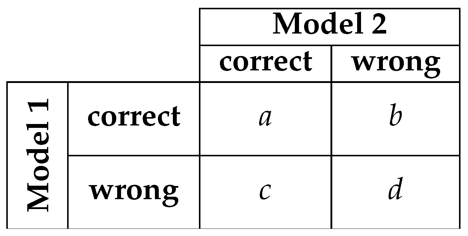
Statistical Significance Tests

To compare the predictive accuracy increase between the L2HNet trained on MapBiomas data and trained on denoised data, we employ McNemar’s test [57]. We formulate our null hypothesis that the predictions between the two classifiers are dependent on each other, and none of the two models performs better [58]. The alternative hypothesis is that the models are significantly different. To perform the test, we create the contingency matrix between the two classifiers, as shown in Figure 4. This matrix shows the number of samples in the validation set that were correctly classified by both classifiers (a), correctly classified by only one of them (b and c), or not captured correctly by either model (c).
We can then formulate our null hypothesis and alternate hypothesis as follows:
H 0 : p ( b ) = p ( c )
H 1 : p ( b ) p ( c )
McNemar’s test statistic is then calculated, with Edwards continuity correction [59]:
χ 2 = b c 1 2 b + c
This follows a chi-squared distribution with a degree of freedom equal to one. We set our significance threshold as α = 0.001 and the critical value as χ α ( 1 ) 2 = 10.828 . If our χ 2 result is significant, meaning higher than the critical value, we can reject the null hypothesis and can accept the alternative hypothesis, i.e., conclude that the difference between the classifiers is significant.

3. Results

In the following subsections, we will present the quantitative assessment of our proposed method, as well as a qualitative analysis to better understand the obtained improvements and limitations of our approach.

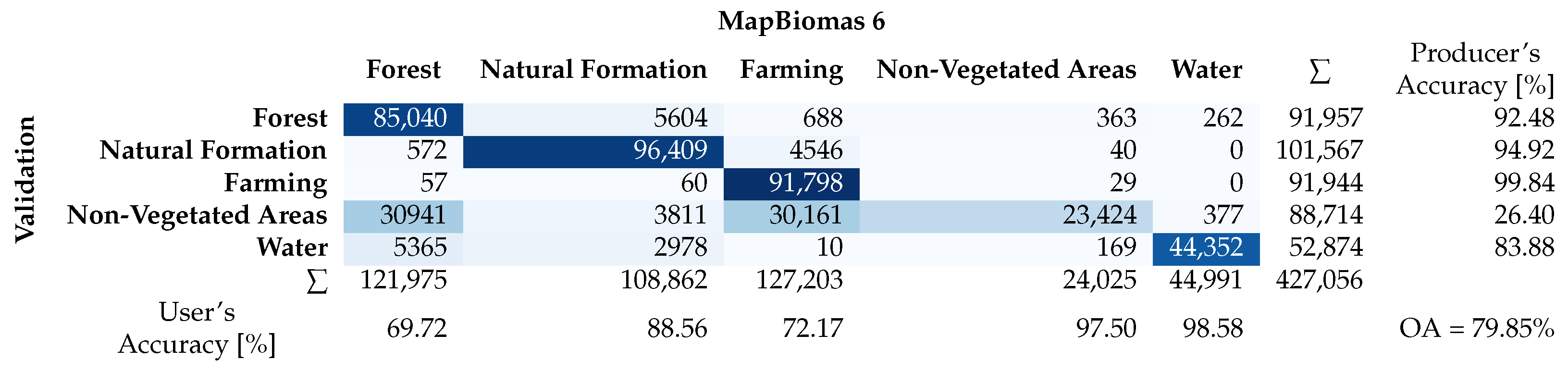
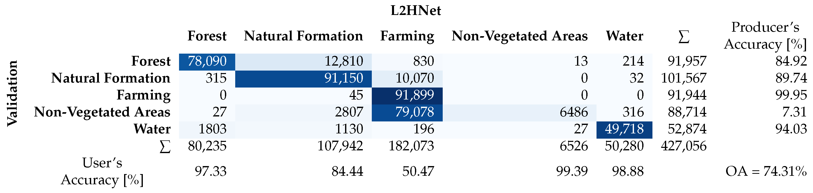
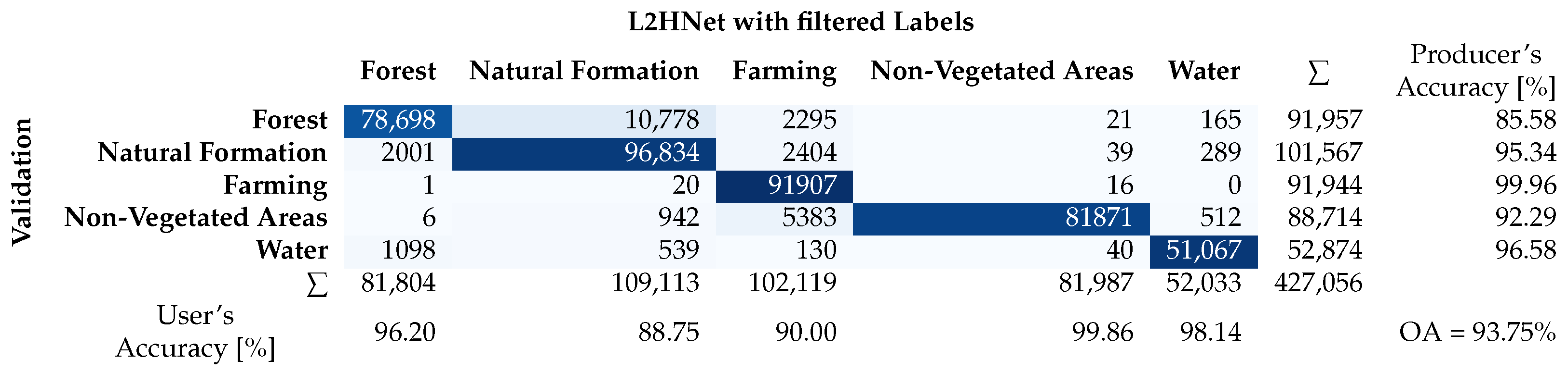
3.1. Quantitative Assessment

In this subsection, we present a quantitative assessment of the results obtained through the application of our data cleaning approach to the Sentinel-2 data with MapBiomas Collection-6 labels. To establish a baseline for comparison, we first validated the accuracy of the MapBiomas data against the manually created validation areas. This initial validation serves as a reference point for evaluating the effectiveness of our data cleaning methodology in improving the overall quality and reliability of the dataset.
The MapBiomas data set reaches an overall accuracy (OA) of 79.85% in the highly accurate validation data set. The resulting confusion matrix is presented in Figure 5. The Farming and Natural Formation classes are the most reliable, with producer’s accuracies (PAs) of 99.84% and 94.92%, respectively. The F 1 -score—which is the harmonic mean of the Producer’s Accuracy and the User’s Accuracy—of the Natural Formation class is also the highest of all five classes, with a value of 91.63%. All F 1 -scores are shown in Table 2. The Non-Vegetated Areas class reached the lowest PA scores in the classification, with only 26.40% of validation pixels coinciding with the label map. Most pixels in that class are detected as the Forest and Farming classes. This is due to the chosen semantics in the validation data. This also leads to a rather high UA in this class, with a score of 97.50%, as the other classes do not become misclassified as Non-Vegetated Areas. Thus, this class reaches the lowest F 1 -score, reaching 41.55% (cf. Table 2). A part of the validation data for this class is bare soil, rather than urban developments. The qualitative validation extent b (cf. Figure A1)shows such an area where validation data were created. The image shows bare soil from a deforested forest, which is classified as Forest in the MapBiomas data, but was interpreted as Other Non-Vegetated Areas. Most misclassifications occur within the Forest class, with a User’s Accuracy of 69.72%, but also significantly within the Farming class, reaching a UA score of 72.17%. The water class is quite confidently classified, with a PA of 83.88%, with some minor misclassifications in the Forest class. These phenomena are further discussed in Section 4.
After applying our proposed correction approach, the OA in the validation areas increases from 79.85% to 89.65%, cf. Figure 6. The confusion of the Non-Vegetated Areas class with other classes is mitigated, and results in a PA of 89.98%, which is a significant change from the baseline 26.40%. The Forest class in the classification map now reaches a higher UA score, 96.60% compared to the previous 69.72%, as those pixels are changed to other classes. The true positives of the Forest class drop significantly, and only reach a PA score of 76.36%. Most of the misclassifications in this class are attributed to the Natural Formation class, and some occurrences in the Farming class. Overall, a positive change is clearly visible in the validation areas.
The scene was also classified with a Random Forest classifier, to assess how robustly it can classify that scene with the given noisy labels. All non-minority classes, i.e., every class but Grassland (cf. Table 1), were randomly down-sampled so that each class has the same amount of input features. This is a necessary step, as the labels are heavily imbalanced, with three classes making up over 90% of all labels. The resulting measures score high in the given validation areas with an OA of 92.55%; see Figure 7. All classes score at least 88% in the PA, with minor misclassifications from Forest to Natural Formation, and from Non-Vegetated Areas to Farming. Random Forest also reaches an F 1 -score of 89.68% in the Natural Formation class and higher in the remaining classes.
Using the L2Hnet learned on the Sentinel-2 data and the MapBiomas labels yields the validation results presented in Figure 8. The classification reaches an overall accuracy of 74.31%, lower than the MapBiomas labels and the other approaches. The biggest confusion occurs from the Non-Vegetated Areas to the Farming, class with a Producer’s Accuracy of only 7.31%, almost completely misclassifying that class. This also leads to a F 1 -score of 13.62% within the Non-Vegetated Area class, see Table 2. However, the model is able to predict the Farming class most confidently with a PA of 99.98%. Further, the misclassification between the Farming and the Non-Vegetated Areas influences the User’s Accuracy score of the Farming class, reaching 50.47%.
In the last experiment, the noisy label data were filtered with our presented approach. The labels were set as unknown when the weight to the neighboring anchor points is lower than a given threshold, as described in Section 2.4. The resulting quantitative validation shows a significant increase in the classification metrics, cf. Figure 9 and Table 2. The overall accuracy rises from 74.31% to 93.75%, an increase of 19.44 percentage points. All producer’s accuracies result in an increase, and are now 85.58% or higher. The misclassifications from the Non-Vegetated Areas class to the Farming class are mitigated, so that the PA of the Non-Vegetated Areas rises from 7.31% to 92.29% compared to the training with the noisy labels. This also increases the UA of the Farming class to 90.00%, compared to the previous 50.47% (see Figure 8). All F 1 -scores are higher than 90%, with significant increases in the Non-Vegetated Areas and Farming classes reaching 95.92% and 94.72%, respectively. Overall, the training of the L2HNet with the filtered data shows the highest overall accuracy, and highest F 1 -scores in all but the Forest class across the presented experiments.
Fisher’s discriminant ratio (FDR) is computed using the data of the whole scene, together with the supposedly noisy label data from MapBiomas. After applying the proposed approach, the FDR is calculated again for each class combination, to assess if the classes are more separable than before. Computing this measure shows the separability of the macro classes of the label data. It can be observed that the Farming class and Water class can be separated most effectively of all the class combinations without any corrections, cf. Table 3a, which reaches a value of 2.67. On the other end, Farming and Natural Formation are not as well separable when assessed with this measure, only reaching a value of 0.84.
After applying the presented approach and relabeling all labels without a threshold, an increase in separability can be observed, as shown in Table 3b. The FDR between Forest and Water decreases slightly, while the FDR between Forest and the remaining classes rise. Most notably is now the separability measure between Forest and Non-Vegetated Areas, which increases to 4.25 from a prior 1.97. Also, the FDR between Farming and Non-Vegetated Areas increased from 1.12 to 2.38, which shows better spectral separation between those classes. This also corresponds to the confusion between those classes with the classification with the L2HNet, and a mitigation of this effect after filtering the labels, as shown in Section 3.2.
The results for McNemar’s test are collected in Table 4. The MapBiomas map itself is also treated as a classifier compared to the validation data. All comparisons between classifiers reach χ 2 values much higher than the critical value of χ 0.001 ( 1 ) 2 = 10.828 , which leads to p-values of much lower than the threshold α = 0.001 . Thus, we can reject the null hypothesis for each combination, and can assume that the differences between the classifiers is significant, and they are not dependent on each other. This is especially interesting for the difference between the L2HNet trained with the noisy labels and our filtered labels. We can conclude that the increase in performance is indeed significant.

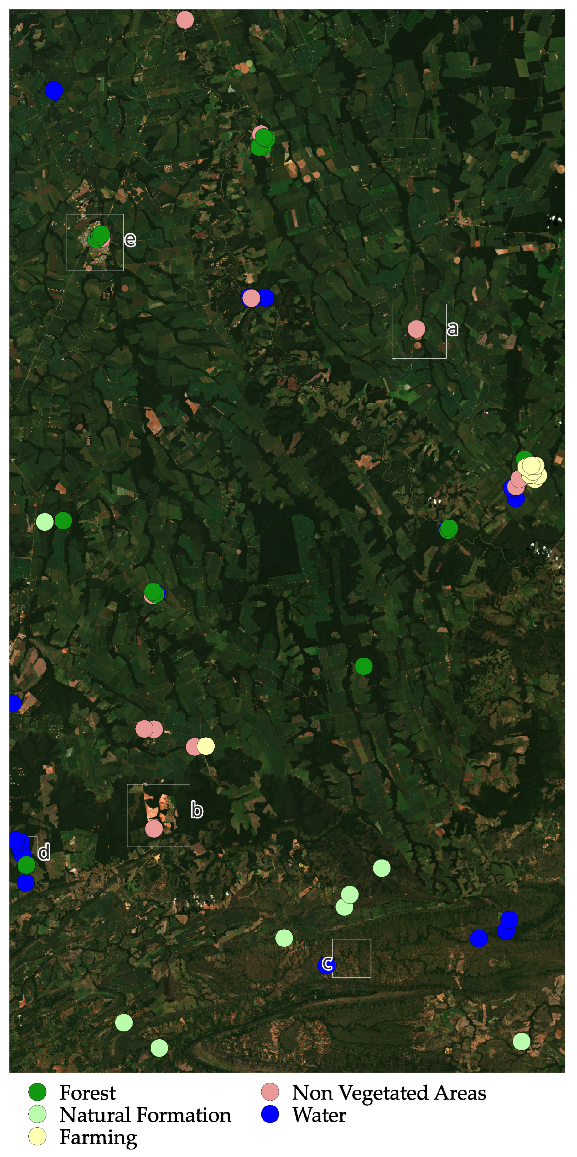
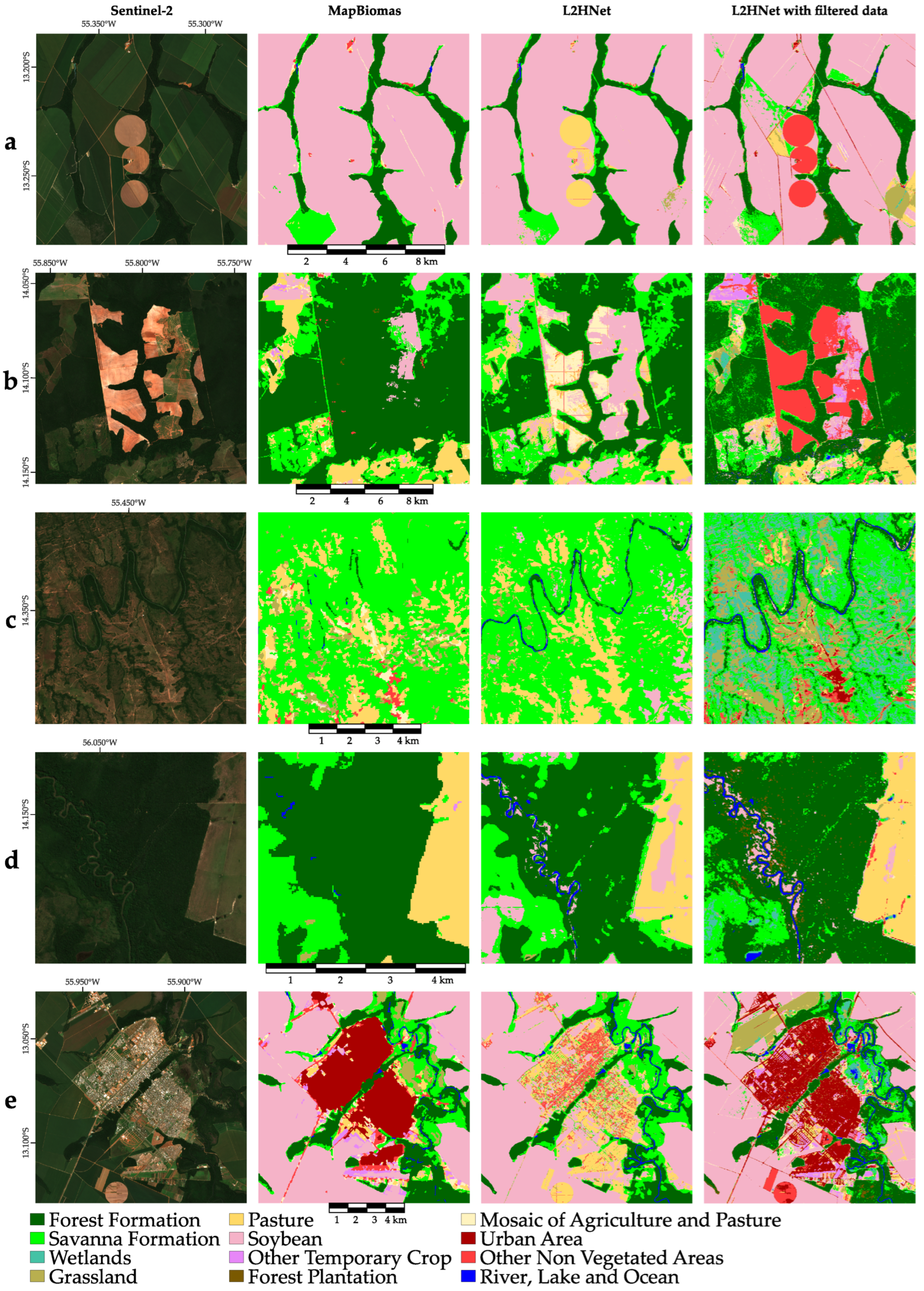
3.2. Qualitative Assessment

For the qualitative visual assessment, five locations showing significant changes after the application of the proposed methods are depicted in Figure 10 and discussed in the following. The bounding boxes of those locations are shown in Figure A1.
Figure 10a shows an image patch which includes farming areas, parts of a forest, some roads, and bare farm land in the form of irrigation circles. The MapBiomas map captures the forested areas with some mixture of forest and savanna formation. One of the roads is partly visible. When relabeling the data with the proposed method, the circular bare lands are reclassified as Other Non-Vegetated Areas. The surrounding fields are classified as a mixture of Soybean, Other Temporary Crops, Mosaic of Agriculture, and Pasture. The Random Forest classifiers robustly covers the agricultural fields, with some misclassifications. The bare land circles are classified as Urban Areas. Classification with the L2HNet yields a labeled map that is smoother than the MapBiomas map, with missing roads. The bare crop circles are classified as Pasture areas.
In Figure 10b, a central part of the true color image is a large portion of deforested area, where parts of it show some sort of vegetation, probably some form of growing crops. To the south of this area, a small river runs across the scene in east–west direction. These two land features are not captured in the MapBiomas map at all. The bare deforested land is classified as Forest, whereas the vegetated areas of it are partly classified as farm land. Pixels that would indicate the river are missing in this map completely. After the application of our presented approach, the bare land is assigned to the Other Non-Vegetated Area class, with the greened parts recognized mostly as Soybean. The river becomes visible, with an almost contiguous coverage. Areas south of the river appear more noisy than the large forest area north of it. Classifying this part with Random Forest yields similar results, especially with respect to the fidelity of the classification. However, the bare land is classified as mixture of Urban Area and Other Non-Vegetated Areas. The deep learning model L2HNet yields a smoother map. The deforested area is mostly classified as Pasture, with the greened parts classified as a contiguous area of Soybean.
The true color image in Figure 10c shows sparsely vegetated ground, a river running across the scene, and some roads present. In contrast, the MapBiomas map shows this scene classified as mostly Savanna, with some farming and natural formation classes in between. Some parts of the bare surface area in the southern part of the scene are attributed to the Other Non-Vegetated Area class. Only a few pixels of the river bank are classified as Water, with the major part being assigned to the Forest class. After the detection of the noisy labels and assigning them to more confident classes, the classification scene changes drastically. The majority of this part of the study area is now assigned to the classes Wetlands, Grassland, and Savanna, which indicate lower density vegetation. The higher density tree cover along the river bed is assigned to the Forest class. The Non-Vegetated Area bare land is expanded from the MapBiomas map and covers more area. Some of the roads also become visible with the proposed approach. The most apparent change is the correct detection of the river. The Random Forest results in a similar map, with less Wetlands and more Savanna. The tree cover along the river is not classified as widely as in our method. Applying the L2HNet, again yields a smoothed map. The bare vegetation classes are assigned to Pasture, and the river is detected similarly to the other methods. Contrary to the other maps, L2HNet detects areas of Soybean in the south-eastern corner.
In the satellite scene of Figure 10d forested areas, as well as some lower density vegetation, farmland, and a river are visible. The MapBiomas LULC map mostly shows Forest, and again does not capture the river well. When correcting the labels, the river becomes clearly classified, similar to the other presented scenes. Also, the vegetated areas without forest cover in the south-west of the scene are changed to the Natural Formation class. After correction of the labels with the presented approach, the river becomes visible, but the area surrounding it are classified as Soybean. The same effect appears in the classification with Random Forest. Here, more pixels in the dense forest area are assigned to Savanna. Again, the L2HNet produces a smoother map, capturing the river and also classifying parts of the Pasture area as Soybean.
The last scene, Figure 10e, also shows a significant change from the original MapBiomas labels to the denoised label map. Again, the waterways become clearly assigned to the Water class, whereas in the original map, those were only partly captured. In the center of the scene, an urban area is visible, and correctly identified as such in the MapBiomas map, and maintained after the cleaning. However, after applying the proposed methodology, more details and finer structures become discernible within that urban area, as well as in the surrounding landscape (i.e., roads).
In the northern part of the settlement, a rather large area is reassigned to the Grassland class. Random Forest yields similar results, with finer structures within the Urban Area becoming visible. The Grassland class is detected here as well. The bare circles in the south of the scene are classified mostly as Urban Area, similar to the scene in Figure 10a. The L2HNet on uncorrected data mostly fails to classify the settlement as such. Most parts are misclassified as Pasture. Finer structures around the settlement are also suppressed in this classification, in contrast to the prediction with prior label correction.
Figure 11 shows the classification results after training the L2HNet with the filtered labels. Here, the labels were corrected and also marked as unknown when the maximum class weight is below 0.3. Regarding the quantitative results, presented in Section 3.1, this lead to a significant increase in accuracy. This effect is also clearly visible in the qualitative assessment. In general, the now resulting classification maps do not appear as smooth as before, but exhibit higher spatial resolution features.
When training the model with the filtered data, roads become more visible, e.g., in Figure 11a. Further, the bare circular regions are now classified as Other Non-Vegetated Areas. North of them, some agricultural land is misclassified as Savanna, and another spot in the eastern part is assigned to Grassland.
The deforested area in Figure 11e is now assigned to Other Non-Vegetated Area, instead of Pasture. The area of classified Soybean is also smaller than with the model learned on the MapBiomas labels. Parts of the forest are now classified less as Savanna, but rather as dense Forest. The classification looks similar to the relabeled version in Figure 10b, but shows more contiguous classifications, rather than single pixels which show another class than their surroundings.
The map significantly changes in Figure 11c when using the filtered data. Fewer regions are classified as Savanna, and are assigned to Wetland and Grassland. Parts of the bare land in the south of the scene are assigned to the non-vegetation classes, instead of Pasture. However, the model detects a rather large area of Urban Area, which is not discernible in the satellite scene. Interestingly, the model successfully detects roads parting from this area as Other Non-Vegetated Areas, as well as in the southeastern part of the scene.
The river running through the scene in Figure 11d, is now more confidently classified. The effect of classifying the surroundings of the river bank as Soybean is now more succinct than before. This also occurred in the classification with Random Forest and the relabeled data, cf. Figure 10d. The area in the southwest is now not classified as Soybean, but rather a mix of Savanna and Wetland.
Changing the training data from MapBiomas labels to the relabeled and filtered labels shows a significant change in L2HNet’s classification of urban settlements. The MapBiomas labels result in misclassification of those areas and are instead mainly assigned to the Pasture class. When using the filtered data, those misclassifications are significantly mitigated, as visible in Figure 11e. Now, the settlement is contiguously detected as Urban Area. The river bank next to the settlement exhibits more detail, with classes such as Wetland appearing.
Conclusively, using the filtered data results in higher quantitative accuracies, cf. Section 3.1, as well as qualitative improvements in the classification when using the L2HNet as a classification model.

4. Discussion

In this paper, a novel approach for the detection of noise in land use and land cover maps is presented. The quantitative and qualitative assessments of the results show promising results for the presented method. When employing the noise cleaning method, the overall accuracy shows a steep increase from 79.85% to 89.65% for the label map in the validation regions. However, this should not be viewed as a final result, but further investigated. The label maps are delivered in a multi level scheme, which discerns multiple classes within five macro classes. The validation regions are created using the macro level classes, while the noise detection and classification is performed on the fine grained classes. This might distort the results, as classes like Urban Area and Other Non-Vegetated Areas are joined into one macro class. The Other Non-Vegetated Areas might comprise areas which exhibit bare soil or rock formation. When misclassification between those classes happen, they do not show up in the quantitative assessment. This is the case with the classification with the Random Forest, which shows high accuracy in this macro class, but the visual inspection showed major misclassifications where bare soil is assigned to the urban class. This shows the importance of qualitatively assessing the results.
One of the major challenges in this study is the prior unknown amount of noise in the data. Other studies mostly use small data sets, which are known to be free of noise, and then introduce artificial, mostly random, noise into the data and its labels as highlighted in Section Learning with Noisy Labels. For example, Tu et al. [44] use a method based on density peaks to detect noise in their data-set, which started clean and was artificially noisified. They show an overall increase in accuracy compared to a baseline support vector machine classification when they filter the noise. However, they only use a small number of samples (20 to 80) and artificially mislabeled instances. This makes it hard to compare to our proposed method, as we use the MapBiomas classification maps, which are derived through machine learning methods and contain an unknown amount of noise. This noise does not solely come from mislabeling a sample, but also a temporal and spatial mismatch between the labels and the Sentinel-2 imagery.
In the resulting maps partly shown in the qualitative assessment (Section 3.2), some phenomena can be observed in the classification maps. The MapBiomas maps mostly suppress fine-grained ground features, such as roads and rivers. A source for this is the rather low resolution of the Landsat imagery used in the project, which has a pixel spacing of 30 m and the spatial filters applied in the methodology. Another challenge in the relabeling is the semantics of the classes. The class Savanna Formation, which usually exhibits low density vegetation, is collected in the macro class Forest. For our study, we switched it to the Natural Formation macro class, as it seemed to fit in there better. It is also noticeable that bare ground from deforestation or crop circles were assigned to the Non-Vegetated classes, both by our approach and the Random Forest classifier. MapBiomas uses a time-series of one year per label map. This hides temporal phenomena like fallow lands and assigns classes which fit to the average representation across a whole year, which is adequate to derive land usage change detection at yearly intervals. When using a scene from one point in time (to classify at a higher temporal resolution or to reduce the amount of data), it becomes hard to discern land use classes that are mostly found in the Farming category of the classification scheme and which are highly variable over the year. To mitigate this problem, the input data also has to be multi-temporal or augmented with other data. These effects also explain the misclassification in the validation areas from Non-Vegetated Areas to Farming, as with the L2HNet, and the assignment to Farming and Forest in the MapBiomas maps. Parts of the validation data for the Non-Vegetated Areas category were created in the deforested area, as visible in Figure 10b and Figure A1, and in areas which show fallow land.
The resulting maps by the L2HNet trained on the MapBiomas data show surprisingly smooth maps, meaning large contiguous areas of one class, as well as a low amount of classes. The smoothed maps seem slightly counter-intuitive, as this network was designed to classify rather high-resolution imagery, but the smoothing in our case seems to happen on a much coarser level. This might occur through the rather large receptive fields within the RP block of the network, which employ convolutions of size 5 × 5 . With a pixel size of 10 m , this results in a rather large receptive field. This suggest that this model might perform with less smoothing at higher resolutions. However, the authors of the original paper proposing the architecture have not shown such effects at the meter level. When analyzing the resulting maps, we found that L2HNet completely omits the Wetlands and the Urban Area classes, and only classifies 221 pixels as Other Temporary Crop. Those classes belong to the minority classes in that scene. This shows an imbalance in the model, which seems to discard underrepresented classes. The map mostly consists of the larger classes, such as Forest, Soybean, Savanna, and Pasture, while the minority classes are mostly omitted. This seems contrary to the model’s purpose, but the original authors only trained it on five LULC classes. The number of classes and their imbalance seem to be a challenge for the model. On the contrary, when the model is trained on the data which was relabeled and filtered with our approach, the minority labels are kept and detected in the resulting maps. The Urban Area class in settlements is correctly assigned, and not mislabeled as a mixture of Pasture and Other Non-Vegetated Areas. This significant change highlights the necessity of noise detection and filter, as presented in this paper. The filtering seems to balance out the incorrect labels from impacting the model and the omission of classes. When testing the predictions of the model trained with MapBiomas and trained with our filtered label, McNemar’s test shows that the improvement between those two results is significant. This is also reflected in the confusion matrices.
Our noise filtering approach with SOMs is somewhat limited, as it omits the spatial relationship of the pixels to their surroundings. However, this seems to have no big impact on the final results, as the corrected map mostly shows contiguous areas of the same class, with only minimal noise. These missing spatial relationships could be integrated in future research, for example by encoding the neighborhood into each of the pixels, or applying spatial filtering techniques on the generated label map. The presented approach will become more computationally expensive as the study region grows. One way to counteract this is to further fit the SOMs with new incoming data, rather than training them from scratch.
Another aspect to discuss is that the chosen validation approach is limited in its application, as we are only able to validate on the macro level of the classification scheme. This introduces some kind of bias as the macro classes do not include important details of labeling errors, such as the misclassification of fallow land to Urban Areas. The MapBiomas validation points would have been a great and accurate resource for this, but they do not include all present classes and are only supplied in level 3 annotation. Nonetheless, our approach shows good results when applied to the MapBiomas data and Sentinel-2 imagery. Much more detail is revealed, especially striking with waterways and roads appearing in the produced maps. It also shows its strengths in the qualitative assessment compared to Random Forest. RF performs slightly better in the quantitative assessment on macro level labels, but the qualitative assessment shows that the RF has, for example, trouble to distinguish the Non-Vegetated Areas micro classes.

5. Conclusions

This work shows that a seemingly good classification map does not hold true when compared with higher resolution imagery, and how to possibly overcome this problem. By coupling self-organizing maps and k-nearest neighbor classification into a noise detection and filtering approach, a significant change towards ground truth can be observed. In the field of remote sensing, such methods for noisy label detection and alleviation could minimize the need for vast manual labeling efforts by recycling older, less reliable maps.
We demonstrate how to improve real-world labels form the MapBiomas project using relatively straightforward techniques, such as self-organizing maps and k-nearest neighbor classification, which can be fused into a noise detection and filtering system. The findings indicate noteworthy enhancements, not only by implementing this technique alone, but also when utilizing its output for subsequent classification with other models such as the L2HNet applied in this study, which showed a significant increase in correct class detection in the accuracy metrics and a visual inspection. Thus, the field of remote sensing can benefit from adopting additional approaches to detect and mitigate noisy labels, and reduce reliance on extensive manual labeling efforts.Such methods can rectify classification errors, enhance the reliability of generated maps, and should be investigated to further improve classification results that are crucially important on an ever changing planet.

Author Contributions

Conceptualization: M.H. and M.B.; Data curation: M.H.; Formal analysis: M.H.; Investigation: M.H.; Methodology: M.H. and M.B.; Project administration: M.B.; Software: M.H.; Supervision: M.B.; Visualization: M.H.; Writing—original draft: M.H.; Writing—review and editing: M.H. and M.B. All authors have read and agreed to the published version of the manuscript.

Funding

The APC is supported by the publication fund of the Technical University of Applied Sciences Würzburg-Schweinfurt (THWS).

Data Availability Statement

All used data in this study is freely available from the Copernicus Data Space (https://dataspace.copernicus.eu/ (accessed on 2 February 2024)) and the MapBiomas project (https://brasil.mapbiomas.org/en/downloads/ (accessed on 2 February 2024)).

Conflicts of Interest

The authors declare no conflicts of interest.

Abbreviations

The following abbreviations are used in this manuscript:
LULCLand Use and Land Cover
SOMSelf-organizing map
OAOverall Accuracy
PAProducer’s Accuracy
UAUser’s Accuracy

Appendix A

Figure A1. Spatial distribution of the manually created validation areas. Extent: UTM tile 21LXE and 21LXF. Area covered: 109.80 km × 209.82 km. The white bounding boxes a–e are showing the areas for qualitative validation (cf. Section 3.2).
Remotesensing 16 02080 g0a1

References

  1. The Nature Conservancy. The Amazon is Our Planet’s Greatest Life Reserve and Our World’s Largest Tropical Rainforest; The Nature Conservancy: Arlington, VA, USA, 2020. [Google Scholar]
  2. Baer, H.A.; Singer, M. The Anthropology of Climate Change: An Integrated Critical Perspective, 2nd ed.; Routledge: London, UK, 2018. [Google Scholar] [CrossRef]
  3. de Area Leão Pereira, E.J.; Silveira Ferreira, P.J.; de Santana Ribeiro, L.C.; Sabadini Carvalho, T.; de Barros Pereira, H.B. Policy in Brazil (2016–2019) threaten conservation of the Amazon rainforest. Environ. Sci. Policy 2019, 100, 8–12. [Google Scholar] [CrossRef]
  4. Carvalho, T.S.; Domingues, E.P.; Horridge, J.M. Controlling deforestation in the Brazilian Amazon: Regional economic impacts and land-use change. Land Use Policy 2017, 64, 327–341. [Google Scholar] [CrossRef]
  5. PRODES—Coordenação—Geral de Observação da Terra. Available online: http://www.obt.inpe.br/OBT/assuntos/programas/amazonia/prodes (accessed on 2 February 2024).
  6. Souza, C.M., Jr.; Z. Shimbo, J.; Rosa, M.R.; Parente, L.L.; A. Alencar, A.; Rudorff, B.F.T.; Hasenack, H.; Matsumoto, M.; G. Ferreira, L.; Souza-Filho, P.W.M.; et al. Reconstructing Three Decades of Land Use and Land Cover Changes in Brazilian Biomes with Landsat Archive and Earth Engine. Remote Sens. 2020, 12, 2735. [Google Scholar] [CrossRef]
  7. Berenguer, E.; Armenteras, D.; Lees, A.C.; Smith, C.C.; Fearnside, P.; Nascimento, N.; Alencar, A.; Almeida, C.; Aragão, L.E.O.; Barlow, J.; et al. Chapter 19: Drivers and ecological impacts of deforestation and forest degradation. In Amazon Assessment Report 2021, 1st ed.; Nobre, C., Encalada, A., Anderson, E., Roca Alcazar, F.H., Bustamante, M., Mena, C., Peña-Claros, M., Poveda, G., Rodriguez, J.P., Saleska, S., et al., Eds.; United Nations Sustainable Development Solutions Network: New York, NY, USA, 2021. [Google Scholar] [CrossRef]
  8. Cherif, E.; Hell, M.; Brandmeier, M. DeepForest: Novel Deep Learning Models for Land Use and Land Cover Classification Using Multi-Temporal and -Modal Sentinel Data of the Amazon Basin. Remote Sens. 2022, 14, 5000. [Google Scholar] [CrossRef]
  9. Zhou, Z.H. A brief introduction to weakly supervised learning. Natl. Sci. Rev. 2018, 5, 44–53. [Google Scholar] [CrossRef]
  10. Han, J.; Luo, P.; Wang, X. Deep Self-Learning From Noisy Labels. In Proceedings of the IEEE/CVF International Conference on Computer Vision, Seoul, Republic of Korea, 27 October–2 November 2019; pp. 5138–5147. [Google Scholar]
  11. Feng, W.; Long, Y.; Wang, S.; Quan, Y. A review of addressing class noise problems of remote sensing classification. J. Syst. Eng. Electron. 2023, 34, 36–46. [Google Scholar] [CrossRef]
  12. Hickey, R.J. Noise modelling and evaluating learning from examples. Artif. Intell. 1996, 82, 157–179. [Google Scholar] [CrossRef]
  13. Brodley, C.E.; Friedl, M.A. Identifying Mislabeled Training Data. J. Artif. Intell. Res. 1999, 11, 131–167. [Google Scholar] [CrossRef]
  14. Nettleton, D.F.; Orriols-Puig, A.; Fornells, A. A study of the effect of different types of noise on the precision of supervised learning techniques. Artif. Intell. Rev. 2010, 33, 275–306. [Google Scholar] [CrossRef]
  15. Liu, Y. Understanding Instance-Level Label Noise: Disparate Impacts and Treatments. In Proceedings of the 38th International Conference on Machine Learning, PMLR, Virtual, 18–24 July 2021; pp. 6725–6735. [Google Scholar]
  16. Lachenbruch, P.A. Discriminant Analysis When the Initial Samples Are Misclassified. Technometrics 1966, 8, 657. [Google Scholar] [CrossRef]
  17. Zhu, Z.; Dong, Z.; Liu, Y. Detecting Corrupted Labels without Training a Model to Predict. In Proceedings of the 39th International Conference on Machine Learning, PMLR, Baltimore, ML, USA, 17–23 July 2022; pp. 27412–27427. [Google Scholar]
  18. Frenay, B.; Verleysen, M. Classification in the Presence of Label Noise: A Survey. IEEE Trans. Neural Netw. Learn. Syst. 2014, 25, 845–869. [Google Scholar] [CrossRef]
  19. García, S.; Luengo, J.; Herrera, F. Dealing with Noisy Data. In Data Preprocessing in Data Mining; García, S., Luengo, J., Herrera, F., Eds.; Intelligent Systems Reference Library; Springer International Publishing: Cham, Switzerland, 2015; pp. 107–145. [Google Scholar] [CrossRef]
  20. Teng, C.M. Correcting Noisy Data. In Proceedings of the Sixteenth International Conference on Machine Learning; ICML ’99; Morgan Kaufmann Publishers Inc.: San Francisco, CA, USA, 1999; pp. 239–248. [Google Scholar]
  21. Verbaeten, S.; Van Assche, A. Ensemble Methods for Noise Elimination in Classification Problems. In Proceedings of the Multiple Classifier Systems; Windeatt, T., Roli, F., Eds.; Lecture Notes in Computer Science; Springer: Berlin/Heidelberg, Germany, 2003; pp. 317–325. [Google Scholar] [CrossRef]
  22. Ghosh, A.; Manwani, N.; Sastry, P.S. Making Risk Minimization Tolerant to Label Noise. Neurocomputing 2015, 160, 93–107. [Google Scholar] [CrossRef]
  23. Gao, W.; Wang, L.; Li, Y.F.; Zhou, Z.H. Risk Minimization in the Presence of Label Noise. Proc. AAAI Conf. Artif. Intell. 2016, 30, 10293. [Google Scholar] [CrossRef]
  24. Thulasidasan, S.; Bhattacharya, T.; Bilmes, J.; Chennupati, G.; Mohd-Yusof, J. Combating Label Noise in Deep Learning Using Abstention. arXiv 2019, arXiv:1905.10964. [Google Scholar] [CrossRef]
  25. Hao, D.; Zhang, L.; Sumkin, J.; Mohamed, A.; Wu, S. Inaccurate Labels in Weakly-Supervised Deep Learning: Automatic Identification and Correction and Their Impact on Classification Performance. IEEE J. Biomed. Health Inform. 2020, 24, 2701–2710. [Google Scholar] [CrossRef]
  26. Patrini, G.; Rozza, A.; Krishna Menon, A.; Nock, R.; Qu, L. Making Deep Neural Networks Robust to Label Noise: A Loss Correction Approach. In Proceedings of the IEEE Conference on Computer Vision and Pattern Recognition, Honolulu, HI, USA, 21–26 July 2017; pp. 1944–1952. [Google Scholar]
  27. Tanaka, D.; Ikami, D.; Yamasaki, T.; Aizawa, K. Joint Optimization Framework for Learning with Noisy Labels. In Proceedings of the IEEE Conference on Computer Vision and Pattern Recognition, Salt Lake City, UT, USA, 18–22 June 2018; pp. 5552–5560. [Google Scholar]
  28. Bahri, D.; Jiang, H.; Gupta, M. Deep k-NN for Noisy Labels. In Proceedings of the 37th International Conference on Machine Learning, PMLR, Virtual, 13–18 July 2020; pp. 540–550. [Google Scholar]
  29. Northcutt, C.; Jiang, L.; Chuang, I. Confident Learning: Estimating Uncertainty in Dataset Labels. J. Artif. Intell. Res. 2021, 70, 1373–1411. [Google Scholar] [CrossRef]
  30. Lee, K.H.; He, X.; Zhang, L.; Yang, L. CleanNet: Transfer Learning for Scalable Image Classifier Training with Label Noise. In Proceedings of the IEEE Conference on Computer Vision and Pattern Recognition, Salt Lake City, UT, USA, 18–22 June2018; pp. 5447–5456. [Google Scholar]
  31. Lu, Z.; Fu, Z.; Xiang, T.; Han, P.; Wang, L.; Gao, X. Learning from Weak and Noisy Labels for Semantic Segmentation. IEEE Trans. Pattern Anal. Mach. Intell. 2017, 39, 486–500. [Google Scholar] [CrossRef]
  32. Thyagarajan, A.; Snorrason, E.; Northcutt, C.; Mueller, J. Identifying Incorrect Annotations in Multi-Label Classification Data. arXiv 2022, arXiv:2211.13895. [Google Scholar] [CrossRef]
  33. Kim, Y.; Yim, J.; Yun, J.; Kim, J. NLNL: Negative Learning for Noisy Labels. In Proceedings of the IEEE/CVF International Conference on Computer Vision, Seoul, Republic of Korea, 27 October–2 November 2019; pp. 101–110. [Google Scholar]
  34. Wilson, D.R.; Martinez, T.R. Instance Pruning Techniques. In Machine Learning: Proceedings of the Fourteenth International Conference; Morgan Kaufmann Publishers: Nashville, TN, USA, 1997. [Google Scholar]
  35. Wilson, D.R. Reduction Techniques for Instance-Based Learning Algorithms; Springer: Berlin/Heidelberg, Germany, 2000. [Google Scholar]
  36. Peikari, M.; Salama, S.; Nofech-Mozes, S.; Martel, A.L. A Cluster-then-label Semi-supervised Learning Approach for Pathology Image Classification. Sci. Rep. 2018, 8, 7193. [Google Scholar] [CrossRef]
  37. Zhu, Z.; Song, Y.; Liu, Y. Clusterability as an Alternative to Anchor Points When Learning with Noisy Labels. In Proceedings of the 38th International Conference on Machine Learning, PMLR, Virtual, 18–24 July 2021; pp. 12912–12923. [Google Scholar]
  38. Tu, B.; Kuang, W.; He, W.; Zhang, G.; Peng, Y. Robust Learning of Mislabeled Training Samples for Remote Sensing Image Scene Classification. IEEE J. Sel. Top. Appl. Earth Obs. Remote Sens. 2020, 13, 5623–5639. [Google Scholar] [CrossRef]
  39. Li, Y.; Zhang, Y.; Zhu, Z. Learning Deep Networks under Noisy Labels for Remote Sensing Image Scene Classification. In Proceedings of the IGARSS 2019—2019 IEEE International Geoscience and Remote Sensing Symposium, Yokohama, Japan, 28 July–2 August 2019; pp. 3025–3028. [Google Scholar] [CrossRef]
  40. Kang, J.; Fernandez-Beltran, R.; Kang, X.; Ni, J.; Plaza, A. Noise-Tolerant Deep Neighborhood Embedding for Remotely Sensed Images with Label Noise. IEEE J. Sel. Top. Appl. Earth Obs. Remote Sens. 2021, 14, 2551–2562. [Google Scholar] [CrossRef]
  41. Aksoy, A.K.; Ravanbakhsh, M.; Demir, B. Multi-Label Noise Robust Collaborative Learning for Remote Sensing Image Classification. IEEE Trans. Neural Netw. Learn. Syst. 2022, 1–14. [Google Scholar] [CrossRef]
  42. Burgert, T.; Ravanbakhsh, M.; Demir, B. On the Effects of Different Types of Label Noise in Multi-Label Remote Sensing Image Classification. IEEE Trans. Geosci. Remote Sens. 2022, 60, 1–13. [Google Scholar] [CrossRef]
  43. Li, Q.; Chen, Y.; Ghamisi, P. Complementary Learning-Based Scene Classification of Remote Sensing Images with Noisy Labels. IEEE Geosci. Remote Sens. Lett. 2022, 19, 1–5. [Google Scholar] [CrossRef]
  44. Tu, B.; Zhang, X.; Kang, X.; Zhang, G.; Li, S. Density Peak-Based Noisy Label Detection for Hyperspectral Image Classification. IEEE Trans. Geosci. Remote Sens. 2019, 57, 1573–1584. [Google Scholar] [CrossRef]
  45. Bahraini, T.; Azimpour, P.; Yazdi, H.S. Modified-mean-shift-based noisy label detection for hyperspectral image classification. Comput. Geosci. 2021, 155, 104843. [Google Scholar] [CrossRef]
  46. Li, Z.; Zhang, H.; Lu, F.; Xue, R.; Yang, G.; Zhang, L. Breaking the resolution barrier: A low-to-high network for large-scale high-resolution land-cover mapping using low-resolution labels. ISPRS J. Photogramm. Remote Sens. 2022, 192, 244–267. [Google Scholar] [CrossRef]
  47. MapBiomas. Em 38 Anos o Brasil Perdeu 15% de Suas Florestas Naturais; MapBiomas: Sao Paulo, Brazil, 2023. [Google Scholar]
  48. Breiman, L. Random Forests. Mach. Learn. 2001, 45, 5–32. [Google Scholar] [CrossRef]
  49. Ronneberger, O.; Fischer, P.; Brox, T. U-Net: Convolutional Networks for Biomedical Image Segmentation. arXiv 2015, arXiv:1505.04597. [Google Scholar]
  50. MapBiomas. MapBiomas General “Handbook” Algorithm Theoretical Basis Document (ATBD) Collection 8; Technical Report; MapBiomas: Sao Paulo, Brazil, 2023. [Google Scholar]
  51. Woodcock, C.E.; Strahler, A.H. The factor of scale in remote sensing. Remote Sens. Environ. 1987, 21, 311–332. [Google Scholar] [CrossRef]
  52. Kohonen, T. Self-organized formation of topologically correct feature maps. Biol. Cybern. 1982, 43, 59–69. [Google Scholar] [CrossRef]
  53. Chang, C.L. Finding Prototypes For Nearest Neighbor Classifiers. IEEE Trans. Comput. 1974, C-23, 1179–1184. [Google Scholar] [CrossRef]
  54. Wittek, P.; Gao, S.C.; Lim, I.S.; Zhao, L. Somoclu: An Efficient Parallel Library for Self-Organizing Maps. J. Stat. Softw. 2017, 78, 1–21. [Google Scholar] [CrossRef]
  55. Theodoridis, S.; Koutroumbas, K. Chapter 5—Feature Selection. In Pattern Recognition, 4th ed.; Theodoridis, S., Koutroumbas, K., Eds.; Academic Press: Boston, MA, USA, 2009; pp. 261–322. [Google Scholar] [CrossRef]
  56. Windrim, L.; Ramakrishnan, R.; Melkumyan, A.; Murphy, R.J.; Chlingaryan, A. Unsupervised Feature—Learning for Hyperspectral Data with Autoencoders. Remote Sens. 2019, 11, 864. [Google Scholar] [CrossRef]
  57. McNemar, Q. Note on the sampling error of the difference between correlated proportions or percentages. Psychometrika 1947, 12, 153–157. [Google Scholar] [CrossRef]
  58. Kumar, P.; Prasad, R.; Choudhary, A.; Mishra, V.N.; Gupta, D.K.; Srivastava, P.K. A statistical significance of differences in classification accuracy of crop types using different classification algorithms. Geocarto Int. 2017, 32, 206–224. [Google Scholar] [CrossRef]
  59. Edwards, A.L. Note on the “correction for continuity” in testing the significance of the difference between correlated proportions. Psychometrika 1948, 13, 185–187. [Google Scholar] [CrossRef]
Figure 1. Study area (blue), spanning the UTM tiles 21LXE and 21LXF, within the bounds of the Amazon basin, or Amazônia Legal (green).
Remotesensing 16 02080 g001
Figure 2. Left: True color rendering of used Sentinel-2 scene with minimal cloud cover. Extent: UTM tile 21LXE and 21LXF. It covers an area of 109.80 km × 209.82 km. Right: MapBiomas Collection 6 label map.
Remotesensing 16 02080 g002
Figure 3. Overview of the proposed method’s workflow. The input data and corresponding labels are flattened to tabular data, where each row represents a single pixel and the columns represent the bands. Those data are then split by their prior labels given by the label map. For each class, a separate SOM is learned to create anchor points for that class. The anchor points are then aggregated. For each data point, the k nearest anchor points in the feature space are searched and weighted. The label of the data point can then be kept, changed (if confident enough), or marked as unknown. The filtered and corrected labels can then be reconstructed as an image.
Remotesensing 16 02080 g003
Figure 4. Example of a contingency matrix for calculation of McNemar’s test.
Remotesensing 16 02080 g004
Figure 5. Confusion matrix using the validation data as ground truth compared to the MapBiomas label map Collection 6.
Remotesensing 16 02080 g005
Figure 6. Confusion matrix using the validation data as ground truth compared to the corrected label map created with the proposed approach. k was set to 10, and the neighbors were weighted by distance.
Remotesensing 16 02080 g006
Figure 7. Confusion matrix using the validation data as ground truth compared to the classification with a Random Forest classifier.
Remotesensing 16 02080 g007
Figure 8. Confusion matrix using the validation data as ground truth compared to the classification with the L2HNet.
Remotesensing 16 02080 g008
Figure 9. Confusion matrix using the validation data as ground truth compared to the classification of the L2HNet with the filtered data as training input.
Remotesensing 16 02080 g009
Figure 10. Qualitative assessment of selected areas showing in the columns: true color image of the used Sentinel-2 imagery, the MapBiomas map, the classification map corrected with the presented approach, the classification with the RF classifier, and the classification with the L2HNet. The rows reflect the five chosen locations for the qualitative assessment. It should be noted that each location is depicted at a different scale. The rows (ae) correspond to the selected areas for qualitative validation marked in Figure A1.
Remotesensing 16 02080 g010
Figure 11. Qualitative assessment of selected areas showing in the columns: true color image of the used Sentinel-2 imagery, the MapBiomas map, the classification map of the L2HNet trained with MapBiomas data, the classification with L2HNet using the filtered labels. The rows reflect the five chosen locations for the qualitative assessment. It should be noted that each location is depicted at a different scale. The rows (ae) correspond to the selected areas for qualitative validation marked in Figure A1.
Remotesensing 16 02080 g011
Table 1. Classes present in the study area given by the MapBiomas label map, together with their percentage in the study area.
Class NameMacro ClassNumber of PixelsProportion of Study Area
Forest FormationForest56,666,05756,666,05724.60%24.60%
Savanna FormationNatural Formation47,971,70150,118,66220.82%21.75%
Grassland57,4370.02%
Wetland2,089,5240.91%
PastureFarming11,936,233121,651,4975.18%52.80%
Soybean103,705,26745.01%
Other Temporary Crop1,739,4050.76%
Forest Plantation198,9540.09%
Mosaic of Uses4,071,6381.77%
Urban AreaNon-Vegetated Areas354,1631,351,9000.15%0.59%
Other Non-Vegetated Area997,7370.43%
River, Lake, OceanWater594,244594,2440.26%0.26%
Σ = 230,382,360
Table 2. F 1 -scores of the macro classes of the validation data for each experiment. Highest scores per class are marked in bold.
MapBiomasDenoisedRandom ForestL2HNetL2HNet (Filtered)
Forest79.50%85.30%92.99%90.70%90.58%
Natural Formation91.63%86.51%89.68%87.01%91.93%
Farming83.78%88.33%92.35%67.08%94.72%
Non-Vegetated Areas41.55%94.67%93.65%13.62%95.92%
Water90.64%97.32%96.25%96.40%97.36%
Table 3. Fisher’s discriminant ratios.
(a) Fisher’s discriminant ratio of the MapBiomas classes (level 1) with the Sentinel-2 data.
WaterNon-Vegetated AreaFarmingNatural Formation
Forest1.481.970.890.89
Natural Formation1.650.880.84
Farming2.671.12
Non-Vegetated Area2.18
(b) Fisher’s discriminant ratio of the corrected labels with the Sentinel-2 data.
WaterNon-Vegetated AreaFarmingNatural Formation
Forest1.304.252.242.90
Natural Formation1.991.781.89
Farming3.252.38
Non-Vegetated Area3.75
Table 4. Results for McNemar’s test for all combinations of classifiers. MapBiomas is seen as a classifier compared to the validation data.
Classifier 1Classifier 2abcd χ 2 -Testp-Value
MapBiomasL2HNet303,27437,74914,06971,96410,820.47 0.001
MapBiomasL2HNet filtered323,55417,46976,823921037,360.31 0.001
L2HNetL2HNet filtered305,64211,70194,73514,97864,775.82 0.001
Disclaimer/Publisher’s Note: The statements, opinions and data contained in all publications are solely those of the individual author(s) and contributor(s) and not of MDPI and/or the editor(s). MDPI and/or the editor(s) disclaim responsibility for any injury to people or property resulting from any ideas, methods, instructions or products referred to in the content.

