MFPANet: Multi-Scale Feature Perception and Aggregation Network for High-Resolution Snow Depth Estimation

Abstract

Accurate snow depth estimation is of significant importance, particularly for preventing avalanche disasters and predicting flood seasons. The predominant approaches for such snow depth estimation, based on deep learning methods, typically rely on passive microwave remote sensing data. However, due to the low resolution of passive microwave remote sensing data, it often results in low-accuracy outcomes, posing considerable limitations in application. To further improve the accuracy of snow depth estimation, in this paper, we used active microwave remote sensing data. We fused multi-spectral optical satellite images, synthetic aperture radar (SAR) images and land cover distribution images to generate a snow remote sensing dataset (SRSD). It is a first-of-its-kind dataset that includes active microwave remote sensing images in high-latitude regions of Asia. Using these novel data, we proposed a multi-scale feature perception and aggregation neural network (MFPANet) that focuses on improving feature extraction from multi-source images. Our systematic analysis reveals that the proposed approach is not only robust but also achieves high accuracy in snow depth estimation compared to existing state-of-the-art methods, with RMSE of 0.360 and with MAE of 0.128. Finally, we selected several representative areas in our study region and applied our method to map snow depth distribution, demonstrating its broad application prospects.

1. Introduction

Snow is a form of water and a crucial component in the water cycle. It is sensitive to temperature fluctuations and arguably a key variable in global climate change [1,2,3]. Against the backdrop of global warming, extreme and adverse weather events are increasingly occurring [4,5,6]. During spring and summer, the snow cover, glaciers, and permafrost of the cryosphere melt at an unprecedented rate. The average snow depth in the European Alps is declining at an almost 10% rate per decade [7]. The rapid melting of snow not only provides abundant freshwater resources for nearby communities but also brings natural disasters such as landslides, soil erosion, and floods [8]. Frequent blizzards and prolonged low temperatures during autumn and winter lead to rapid snow accumulation, posing threats to agriculture and livestock while increasing the likelihood of avalanches [9]. Snow depth serves as one of the most intuitive indicators to warn against natural disasters like avalanches and to assess snow melt changes. Therefore, the research value of monitoring snow depth is exceptional.

However, due to the lack of meteorological stations in high-altitude or uninhabited areas where snow persists throughout the year, comprehensive snow depth monitoring in frigid regions still lacks effective measures [10,11]. Consequently, exploring wide-ranging, high-resolution, and high-precision methods for snow depth estimation has become a hot research topic in various fields such as remote sensing, hydrology, energy planning, and ecology. Remote sensing technology stands as an effective way to perceive large-scale snow depth information [12,13,14]. However, snow depth estimation based on passive microwave remote sensing is limited by low spatial resolution and large differences (1–25 km), so the snow depth estimation can only be made at the kilometer level, generally [15,16]. In recent years, despite numerous scholars conducting a series of downscaling research, it seems that the spatial resolution has reached a bottleneck of around 500 m [17]. With the development of satellite remote sensing technology, a large number of active microwave remote sensing satellites have appeared. High-resolution active microwave remote sensing data, with their exceptional penetration capabilities and immunity to any weather conditions, hold vast potential in the field of snow depth estimation research [18,19,20]. For instance, the open-source SAR images from the Sentinel-1 satellite launched in 2014 have a spatial resolution of up to 10 m and possess extremely strong penetration capabilities, capable of penetrating cloud and snow layers. Furthermore, considering more snow-related influencing factors and fusing underlying surface information closely associated with snow cover is also meaningful for achieving higher precision in snow depth estimation. Especially in the deep learning-based method, multi-source data fusion has been verified as an effective method for snow depth estimation.

Snow depth estimation based on SAR (an active microwave remote sensing) can be divided into traditional methods and deep learning-based methods. The traditional method holds that snow is an isotropic heterogeneous medium, and the Polarimetric Synthetic Aperture Radar (PolSAR) uses the differences in the propagation speed of HH and VV polarized signals within the snow layer to generate the Co-Polarization Phase Difference (CPD). By establishing the relationship between CPD and snow depth, a snow depth retrieval model can be constructed [21,22]. Simultaneously, interferometric techniques are widely applied in the construction of snow parameter inversion models. Utilizing interferometric processing of more than two SLC images from the same area allows the retrieval of millimeter-level surface elevation change information. Differential SAR Interferometry (D-InSAR) uses the geometric correlation between the slant range difference generated by microwave penetration through the snow layer and the interferometric phase of the snow layer to acquire snow-related information [23,24]. Yang and Li [25] assimilated snow depth from D-InSAR data using an Ensemble Kalman Filter. Lievens et al. proposed a physical model to estimate snow depth using SAR images, employing backscattering $\sigma 0$ to estimate snow depth in Northern Hemisphere mountain ranges, demonstrating a strong correlation between the $\sigma VH$/$\sigma VV$ ratio and snow depth [26]. Recently, as data-driven approaches, deep learning-based methods can leverage neural networks to learn nonlinear relationships inherent in sample datasets, and these techniques have found widespread applications in the field of remote sensing [27,28,29,30]. An increasing number of scholars have applied deep learning in snow depth research, achieving significant success. Yu et al. demonstrated the advantages of deep learning by examining changes in snow depth before and after blizzards in the Texas region using SAR images [31]. Rodrigo Caye Daudt and colleagues achieved success in snow depth mapping and snow disaster risk assessment in Switzerland by fusing SAR images with multi-spectral optical imagery data, employing recurrent neural networks [14].

Optical remote sensing can accurately judge snow pixels, but it is difficult to obtain snow parameter information. SAR remote sensing can actively transmit microwave signals to obtain backscattered signals reflected by the target. It has penetration power for clouds and fog, and can penetrate a certain thickness of snow to obtain snow and snow information. SAR remote sensing has higher spatial resolution than passive microwave remote sensing, so it is suitable for high-resolution snow parameter monitoring. At present, researchers have conducted a lot of research on the estimation of snow parameters using SAR remote sensing. Varade et al. [32] proposed a method for estimating snow density using dual-temporal fully polarized C-band radar data, and Singh et al. [33] proposed a C-band SAR snow density estimation algorithm. Based on dielectric constant inversion, Rodrigo Caye Daudt et al. [14] realized high-resolution snow depth estimation in Switzerland based on C-band SAR-GRD data combined with optical remote sensing data. These related works provide a reliable basis for the data selection of this work.

In this work, taking advantage of the excellent identification capability of optical remote sensing for snow-covered areas and the exceptional penetration capability of high-resolution active microwave remote sensing, coupled with the all-weather immunity, a SAR remote sensing image was combined with a multi-spectral optical remote sensing image and land cover data to estimate snow depth in high-latitude regions of Asia. We present a novel ‘area-to-point’ deep model, both in terms of dataset and methodology.

The major contributions can be summed up as follows:

• Constructing a multi-source dataset: This work contributes a snow cover remote sensing dataset for high-latitude regions of Asia. This dataset fuses multi-spectral optical satellite images, SAR images, and land cover distribution images. Ground snow depth measurements from meteorological stations are used as the ground truth.
• Proposing a multi-scale neural network: Unlike ‘point-to-point’ predictions ignore spatial characteristics, our model is an ‘area-to-point’ snow depth estimation deep model. The proposed network comprises a multi-branch feature extraction unit (MBFE), a multi-scale feature atrous aggregation module (MSFAA), and a high- and low-level feature fusion module (HLF). These components endow the new model with multi-scale feature perception capabilities, which is particularly advantageous in reducing non-snow area spatial interference, thereby achieving high accuracy snow depth estimation.
• Mapping snow depth distribution: By these optimal parameters of our model, a snow depth distribution map with a high resolution of 320 m in the study area is shown. It can be predicted that based on our method, high-resolution snow depth maps in any area of interest can be generated.

2. Methodology

In this work, the estimation of snow depth can be regarded as a regression task in deep learning. Feature extraction is a key step, which directly affects the estimation results. Due to the small-size nature of the input images, the information diminishes after several convolutional operations. To reduce such information loss, we propose a dual-branch structure based on the residual network called the MBFE unit. It contains two branches, where each branch of the downsampling sequence is not the same, and can extract and fuse different snow feature information. In addition, we introduce an MSFAA module, which contains multiple receptive fields. It uses the concept of pyramid pool to aggregate features. The design of cross-pixel extraction features can effectively reduce the non-snow interference of low gray values in the image. Then, we design the HLF module, which aims to integrate the extracted low-level and high-level features; this module helps to avoid the loss of semantic information caused by the simple combination of different scale features. Finally, we use the global average pool for the aggregated features, and then use the fully connected layer to output the estimated snow depth value. We employ dropout regularization to enhance the network’s robustness and generalization ability. The overall network structure can be seen in Figure 1.

2.1. Multi-Branch Feature Extraction Unit (MBFE)

We use deep learning techniques to focus on learning and recognizing the characteristics of snow at different depths. Our objective is to explore the correlation between different input image sources and snow depth values, thereby enhancing prediction accuracy. Generally, deeper networks tend to possess stronger capabilities in representing snow characteristics, allowing them to learn more complex and abstract snow features. However, as the network depth increases along with the parameters, issues such as vanishing or exploding gradients may arise. The ResNet proposed by He et al. [34] effectively addresses this problem. Here, we base our method on the residual network, using a dual-branch residual network structure as the main framework to extract and fuse features of different levels. The expression of the residual unit in the residual block is given as follows:

$$x_{i+1}=x_i+Con{v}_{i+1}\left\{\mathrm{Re}LU\left[Con{v}_i(xi)\right]\right\}$$

(1)

where $x_i$ is the input matrix of the first residual unit, $x_{i+1}$ is the output matrix of the residual unit, $Con{v}_{i+1}$ and $Con{v}_i$ represent convolution operations, and function represents the nonlinear function ReLU.

The low-level semantic information in snow remote sensing images is typically closely associated with fundamental features of snow, such as snow color and texture of the snow cover. The high-level semantic information involves a multi-dimensional understanding of the internal structure of snow and various parameters related to snow. Therefore, extracting multi-scale snow features is crucial for identifying snow and exploring snow depth information. We designed the MBFE unit as the backbone to explore semantic information at different depth levels of snow.

We adopted a dual-branch convolutional neural network, configuring the downsampling order of residual units within the two branches to be opposite to each other. To achieve feature enhancement and complementarity, after the first convolutional downsampling, we set a concatenation operation on two low-level features. Following the second convolutional downsampling, we combined high-level features extracted from three distinct branches. We were able to effectively verify the effectiveness of this design in the experiment part. Through the MBFE unit, we were able to obtain two different scale feature maps. The details of each layer in MBFE can be seen in Figure 2.

2.2. Multi-Scale Feature Atrous Aggregation Module (MSFAA)

To extract features comprehensively and minimize the interference of non-snow factors, we incorporated five MSFAA modules into the network. The goal is to extract multi-scale snow features acquired through the MBFE unit using various receptive fields. The module consists of three depth-separable convolutions with different dilation rates with a kernel of 3 × 3, a convolution with a kernel of 1 × 1, and a 2 × 2 average pooling operation; the output of the module concatenates the features obtained from the five branch operations, thereby increasing the number of channels. For specific details, they can be seen in Figure 3. Firstly, the design of dilated convolutions allows the extraction of snow features across pixels at different scales, effectively reducing the interference from speckle-like non-snow artifacts in the image. This is crucial for further enhancing the extraction capability of various snow features in our task. We were inspired by PSPnet and structured it in a pyramid-like shape [35], effectively consolidating snow features across different scales and deep semantic information. In addition to the design of dilated convolutions, the input feature images are also subjected to average pooling and 1 × 1 convolution operations. Using average pooling can better focus on the spatial information of snow in the image, enhance global snow features, and using 1 × 1 convolution can enhance the input features by fusing semantic information from different feature dimensions, which helps to better estimate the snow depth value in the region. We choose to use depth separable convolution in the MSFAA module to reduce the number of parameters while ensuring the accuracy of the estimation.

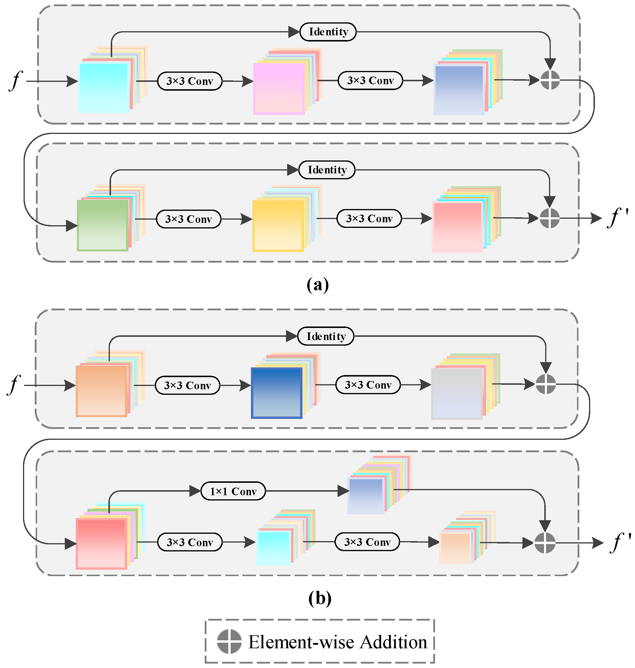
2.3. High- and Low-Level Feature Fusion Module (HLF)

Previously, we discussed that the characteristics of different scales can represent snow from different angles. Inspired by the work of Dai et al. [36], Chen et al. [37], and others, we propose the HLF module, aiming to effectively integrate two distinct scales of features. This design enhances the interaction between different channels within the model. The structural details of the HLF module can be seen in Figure 4.

Specifically, we designed two branches, where one branch inputs high-level semantic information $U_1$ and the other branch inputs low-level $U_2$, and these two branches do not know each other’s feature information. For the low-level features, we designed two sub-branches. The first sub-branch initially applies a depth separable convolution with a kernel size of 3 × 3, dilation rate of 2, then $U_{22}$ is obtained by sigmoid activation. The other sub-branch is first doubled by Avgpool with a kernel of 3 × 3 and stride of 2, and then $U_{21}$ is obtained by sigmoid activation. For high-level features, two sub-branches are similarly arranged. These sub-branches first enhance features through depth-separable convolutions with a 3 × 3 kernel and a dilation rate of 2, obtaining $U_{11}$, the other branch samples through bilinear interpolation to obtain $U_{12}$ with the same size as the low-level feature map subsequently. We set a weighted operation on feature maps $U_{11}$ and $U_{21}$, obtaining $H_1$ through bilinear interpolation, the feature map $U_{12}$ and $U_{22}$ were weighted to obtain $L_1$ at the same time. The final step involves adding the same-sized $H_1$ and $L_1$ feature maps. Initially, adjusting the channel numbers through a 1 × 1 kernel convolution is performed, followed by two layers of 3 × 3 kernel dilated convolution with a dilation rate of 4 to enhance the fused features. The arithmetic operations involved in the HLF module can be expressed as follows:

$$U_{11}=R(BN(DsCon{v}_{3\times 3}(U_1)))$$

(2)

$$U_{12}=Up(R(BN(DsCon{v}_{3\times 3}(U_1))))$$

(3)

$$U_{21}=f(A{p}_{3\times 3}(U_2))$$

(4)

$$U_{22}=f(R(BN(DsCon{v}_{3\times 3}(U_2))))$$

(5)

$$H_1=Up\left[U_{11}\otimes U_{21}\right]$$

(6)

$$L_1=U_{12}\otimes U_{22}$$

(7)

$$O_t=Con{v}_{1\times 1}(H_1+L_1)$$

(8)

$$O=Con{v^2}_{3\times 3}(O_t)+O_t$$

(9)

where $DsCon{v}_{3\times 3}$ denotes a depth separable dilated convolution with a kernel size of 3 × 3 and a dilation rate of 2, $Con{v}_{1\times 1}$ denotes a 1 × 1 2D convolutional kernel, $Con{v^2}_{3\times 3}$ denotes a two-layer convolution with dilation rate of 4 and kernel of 3 × 3, $A{p}_{3\times 3}$ represents a 3 × 3 average pooling operation, $BN$ represents bilinear interpolation upsampling, R represents the ReLU activation function, f represents the non-linear activation function sigmoid, $U_1$ is the input high-level feature, $U_2$ is the input low-level feature, $O_t$ is a temporary output in the module, and O is the fused features obtained through this module.

The HLF module weights the feature maps through a non-linear activation function sigmoid, merging deep semantic information and shallow detailed information, thereby complementing the feature representations of the two branches. It can effectively avoid issues such as distortion of two-level semantic information and loss of diversity caused by simple combinations.

3. Experiments

3.1. Study Area and Dataset

The study area of this work is located in the high-latitude regions of Asia, including the Qinghai–Tibet Plateau, Xinjiang and Gansu province $(21.{28}^{°}$N∼$48.{05}^{°}$N, $81.{33}^{°}$E∼$102.{67}^{°}$E). As shown in Figure 5, this area is far from the ocean, with low average temperatures in autumn and winter, and exhibits a markedly continental arid and semi-arid climate. With high altitude and complex terrain, it is an optimal choice for our research on snow depth.

To our knowledge, there is currently a lack of publicly available high-resolution snow remote sensing datasets for research on snow depth in the high-latitude regions of Asia, especially radar remote sensing data. In this work, we combined data from several different sources for input data. We chose satellite data from Sentinel-1A launched in 2014 and Landsat-8 launched in 2013, integrating pre-processed multi-spectral optical remote sensing data, SAR images, land cover data around the meteorological stations from 2014 to 2017. As we mentioned earlier, the resolution of estimating snow depth using passive microwave downscaling can reach approximately 500 m. Considering the high-resolution advantage of highlighting radar remote sensing in snow depth estimation tasks, combined with our computing power and memory resources, we decided to crop the registered remote sensing images to 32 × 32, representing 320 m × 320 m on the ground, and the snow remote sensing dataset (SRSD) with a resolution of 30 m was prepared. We used horizontal and vertical rotation as data augmentation strategies. Finally, a total of about 10,000 eight-channel snow remote sensing data were obtained. We divided the training set and the test set according to the ratio of 4:1. The training set contains 8889 images, while the test set contains 1846 images. Compared with the single point estimation, our model receives the snow information of a small area as input and learns the spatial pattern of snow so that it has better estimation effect in the face of complex snow conditions. While ensuring high resolution, it also provides spatial information of snow for the model and ensures the credibility of the snow depth value of the label. If the resolution of a single-point pixel is high enough, it can achieve higher-resolution snow depth estimation. We used the snow depth observation data from meteorological stations within the research area as labels. Figure 6 shows the amount of data in the dataset at different depths through a bar graph. Figure 7 displays a group of example images from our dataset. The following will introduce the data sources of this work.

3.1.1. SAR Images

The Sentinel-1 GRD data, with a resolution of 10 m, are composed of C-band SAR images with single VV polarization, downloaded from https://dataspace.copernicus.eu/ (accessed on 1 June 2023). The Sentinel-1 data downloaded in this work are processed using ESA’s SNAP 8.0 software. The meteorological events captured by the images, such as changes in solar light, cloud cover, etc., show strong robustness, which makes them a reliable and timely tool for earth observation. After orbit correction, thermal noise removal, radiometric calibration, terrain correction, and other operations, the pre-processed SAR image is obtained.

3.1.2. Multi-Spectral Optical Satellite Images

Under clear and cloudless weather conditions, we selected and downloaded optical images of the study area that coincide with the visits of the Sentinel-1 satellite, with a resolution of 30 m. We selected four bands from the visible and near-infrared spectral range of the Landsat-8 satellite, and performed band fusion and resampling operations using ENVI 5.3 software. This process generated four channels optical images with a resolution of 10 m. Our multi-spectral optical images were downloaded from the Landsat-8 satellite https://earthexplorer.usgs.gov/ (accessed on 1 June 2023).

3.1.3. Land Cover

Different land cover types have different effects on the backscattering of snow. The backscattering coefficient of snow on bare land is higher than that under vegetation cover [38]. Therefore, the introduction of snow underlying surface land cover information is necessary for the detection of snow depth information. The data are produced by Impact Observatory, Microsoft and Esri, and are generated using the Impact Observatory’s deep learning AI land classification model with a resolution of 10 m, providing three channels of information for the dataset, downloaded from https://livingatlas.arcgis.com/landcoverexplorer/(accessed on 1 June 2023). The rightmost image in Figure 7 shows a scene of land cover in our study area. The land cover data we used classify the ground into categories such as water, trees, crops, ice, built-up areas, bare ground, rangeland, flooded vegetation, etc.

3.1.4. Ground Observation

We obtained the daily surface snow depth observation data from the National Meteorological Information Center http://data.cma.cn/site (accessed on 16 May 2020), and regarded them as the objective truth value as the label data for model training. The obtained observation data cover the daily monitoring data of more than 200 meteorological stations in the study area from 2014 to 2017, including station numbers, station longitude and latitude, and the snow depth values observed on that day. Based on the overlapping visit frequency of SAR remote sensing and optical remote sensing, we used the daily observed snow depth values of 23 stations as labels to complete the preparation of the SRSD dataset; the SRSD dataset we prepared can cover 0∼42 cm of snow depth, which can theoretically estimate the depth of light snow and deep snow.

3.2. Experimental Parameter Setting

All of the reported experiments were conducted using PyTorch and configured with a Nvidia GeForce RTX4070Ti GPU card. The optimizer used is adaptive moment estimation (Adam), and the learning rate strategy is the “ploy” strategy, the formula of which can be defined as:

$$\mathrm{lr}=\mathrm{base}\_\mathrm{lr}\times (1-\frac{\mathrm{epoch}}{\mathrm{num}\_\mathrm{epoch}}{)}^{\mathrm{power}}$$

(10)

where lr is the updated learning rate, base_lr is the baseline learning rate, epoch is the quantity of iterations, num_epoch is the maximum number of iterations, and power controls the shape of the curve (usually it is greater than 1). In our model, power is set to 0.9, and we finally fixed the epoch number to 250. We did not use pre-training parameters during the training process. We set the batch size to 64. In order to prevent overfitting of the model, we adopted various methods in the design, including data augmentation, dropout, and normalization. In addition, we also designed a tenfold cross-validation experiment, by taking turns selecting onefold of data as the test set and using the remaining ninefold data for training to ensure the stability of the model and the reliability of the experimental results. The loss function used in this work is MSE. The equation can be listed as:

$$MSE(y,\stackrel{\wedge }{y})=\frac{1}{N}\sum _{\mathrm{i}=1}^N{({\stackrel{\wedge }{y}}_i-y_i)}^2$$

(11)

In order to evaluate the performance of our network in SRSD datasets, we chose four main metrics: root mean squared error (RMSE), positive mean error (PME), negative mean error (NME), and coefficient of determination ($R^2$). And their equations can be defined as:

$$RMSE(y,\stackrel{\wedge }{y})=\sqrt{\frac{1}{N}\sum _{i=1}^N{(y_i-\stackrel{\wedge }{y_i})}^2}$$

(12)

$$MAE(y,\stackrel{\wedge }{y})=\frac{1}{N}\sum _{i=1}^N\left|y_i-\stackrel{\wedge }{y_i}\right|$$

(13)

$$PME=\frac{1}{p}\sum _{i=1}^p(\stackrel{\wedge }{y_i}-y_i),\stackrel{\wedge }{y_i}>y_i$$

(14)

$$NME=\frac{1}{r}\sum _{i=1}^r(\stackrel{\wedge }{y_i}-y_i),\stackrel{\wedge }{y_i}<y_i$$

(15)

$$R^2={[\frac{N-1}{N}\sum _{i=1}^n(\frac{y_i-\mu (y_i)}{\sigma (y_i)})(\frac{\stackrel{\wedge }{y_i}-\mu (\stackrel{\wedge }{y_i})}{\sigma (\stackrel{\wedge }{y_i})})]}^2$$

(16)

where y means the model estimated snow depth value, and $\stackrel{\wedge }{y}$ means the station observed snow depth value. $\mu (•)$ denotes the mean operator, $\sigma (•)$ denotes the standard deviation operator, and N denotes the data sample size. p and r are the number of samples whose measured snow depths are greater and less than the retrieved snow depth. Among them, $R^2$ can well characterize the correlation between y and $\stackrel{\wedge }{y}$.

3.3. Ablation Studies

In this section, we conduct a series of ablation experiments on MFPANet to examine the rationality and effectiveness in the structural design of its modules and the selection of data source. Firstly, we test the MBFE unit and then we gradually add the designed modules MSFAA and HLF to the model. We show the experimental results through a series of tables, and accordingly give the parameters (Params), computational complexity (FLOPs), and other indicators to consider our model.

MBFE Ablation: We experimentally compare the prediction performance of MBFE under different branch numbers. The experimental results can be seen in

Table 1. Performance comparison of MBFE unit using different branch combinations. (Bold represents the best result).

Method	RMSE (↓)	MAE (↓)	PME (↓)	NME (↓)	${\mathit{R}}^2$ (↑)	Params (M)	FLOPs (G)
MBFE—single branch (branch1)	1.192	0.524	0.504	−0.548	0.989	0.85	0.143
MBFE—two branches (branch1 + branch2)	1.008	0.393	0.361	−0.444	0.991	2.25	0.286
MBFE—three branches (branch1 + branch2 + branch3) (Ours)	0.903	0.283	0.286	0.281	0.992	6.75	0.573

. Due to the different down-sampling sequences set in the residual blocks of the two different branches (branch1 and branch2), the two branches will extract different snow features, respectively. By comparing the experimental results of MBFE-single branch and MBFE-two branches, it can be found that this design can well realize the complementarity and enhancement of snow semantic information at the same scale, alleviate the excessive loss of snow semantic information in the down-sampling process, and greatly improve the prediction ability of the network. Comparing the experimental results, the addition of branch3 helps to partially compensate for the semantic information lost during the first downsampling. Therefore, we consider that the MBFE unit is suitable as our backbone to extract features.

MSFAA Ablation: We set up five MSFAA modules in the network. In this part of the experiment, we first conducted single-scale (MBFE + 3MSFAA) and multi-scale (MBFE + 5MSFAA) experiments. Compared with the experimental results in

Table 2. Step-by-step performance comparison of networks using designed modules (MSFAA and HLF). (Bold represents the best result).

Method	RMSE (↓)	MAE (↓)	PME (↓)	NME (↓)	${\mathit{R}}^2$ (↑)	Params (M)	FLOPs (G)
MBFE	0.903	0.283	0.286	−0.281	0.992	6.75	0.57
MBFE + 3MSFAA	0.878	0.231	0.175	−0.273	0.992	8.38	0.67
MBFE + 5MSFAA	0.541	0.146	0.155	−0.138	0.995	10.03	0.74
MBFE + 5MSFAA + HLF (Ours)	0.360	0.128	0.124	−0.129	0.997	13.60	1.36

, we found that the fusion of different scale features makes the predicted RMSE decrease by 0.337, and the estimation effect is significantly improved. On the other hand, by comparing the experimental results, we can also found that the estimation ability of our model is improved after adding the MSFAA module under the premise of single scale or multi-scale, which proves that this module is effective and also verifies that the fusion of multi-scale snow features is necessary for the snow depth estimation task.

HLF Ablation: We achieved satisfactory estimation results by simply superimposing and combining features from two scales (MBFE + 5MSFAA). After that, we no longer simply combine features of different scales but use the HLF module to fuse features of two scales (MBFE + 5MSFAA + HLF). By comparing the two experimental results in Table 2, it can be found that the introduction of the HLF module reduces RMSE by 0.189, which verifies the effectiveness of the HLF module, avoids the loss of information combination at different scales, and better integrates snow semantic information at different scales.

Data Ablation: In this section, we conduct a data ablation study on the multi-source data we made, using the proposed MFPANet. We separate the eight-channel dataset SRSD into a four-channel dataset (SAR + Land cover), a five-channel dataset (SAR + multi-spectral optical satellite) and a seven-channel dataset (multi-spectral optical satellite + Land cover) by encoding. In addition to the number of channels, the ablation dataset is consistent with the original dataset in the scale of the training set and test set. By this way, we discuss the contribution of each data source to snow estimation in our multi-source dataset, and prove that our strategy of fusing multi-source data is necessary.

Table 3. Performance comparison of data combination approaches. (Bold represents the best result).

Data Combination Approach	Channels	RMSE (↓)	MAE (↓)	R2 (↑)
SAR + Land cover	4	9.285	7.022	0.320
SAR + Multi-spectral optical	5	0.981	0.190	0.991
Multi-spectral optical + Land cover	7	0.768	0.172	0.994
Multi-spectral optical + SAR + Land cover (Ours)	8	0.360	0.128	0.997

shows the experimental results of data ablation; it strongly proves the effectiveness of our data selection combination. According to these results, it is clear that if we only combine SAR images and land cover data, in the absence of multi-spectral optical remote sensing to provide spatial information of snow cover, the effect of our network fitting snow depth true value is very poor, and the model can hardly perceive the existence of snow cover. On the other hand, with the combination of the SAR image and multi-spectral optical image or the combination of multi-spectral optical data and land cover data, the estimation effect is far less than the combination of SAR images, multi-spectral optical images and land cover data. It can be inferred that each data source is contributing to snow depth estimation. Optical remote sensing images can provide information on the snow cover surface to help perceive and identify snow cover. Land cover provides underlying surface information. SAR can penetrate into the interior of the snow layer, providing information about the internal structure of the snow and the backscattering intensity from the underlying surface. We show the scatter plot of the model’s estimation ability under different data combinations. It can also be seen from Figure 8 that the model has a better fitting effect based on our data selection.

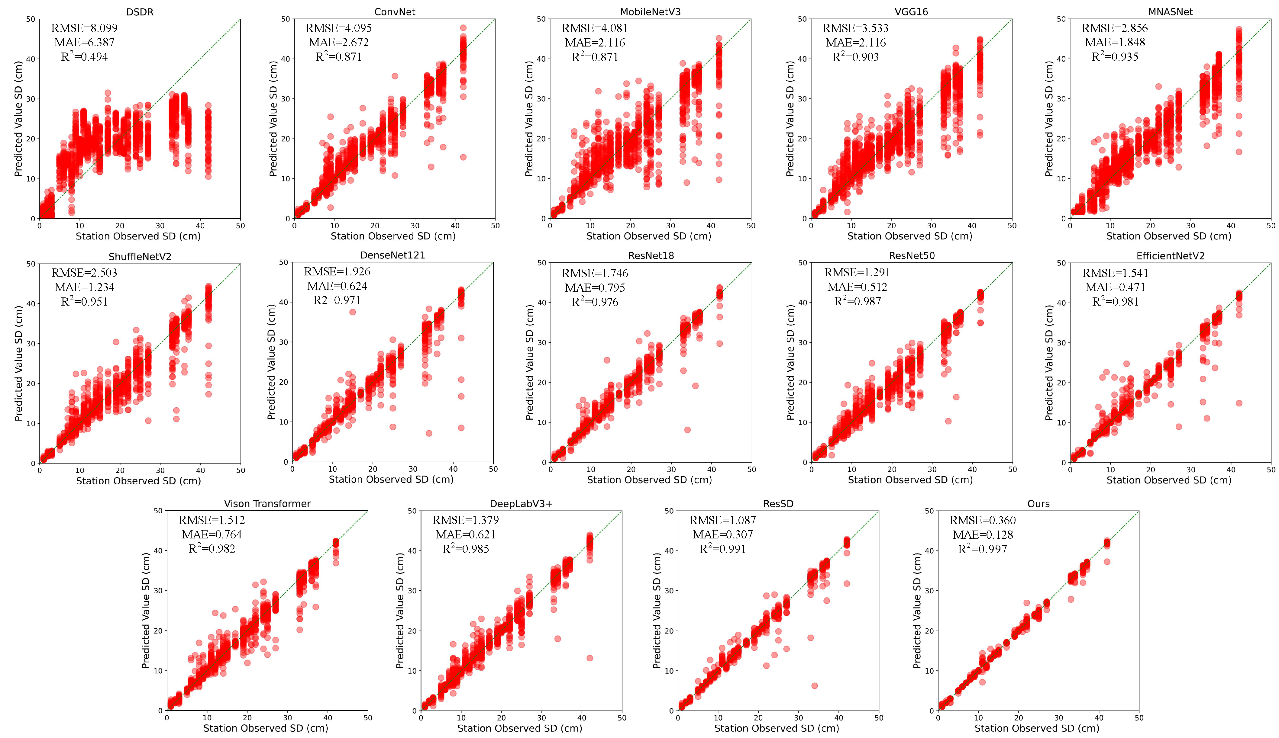
3.4. Comparative Analysis

Firstly, through an extensive literature review, we discovered several outstanding deep learning methods that use multi-source remote sensing data for snow depth estimation. They are adaptable for comparison on our SRSD dataset. We selected DSDR [17], ConvNet [39], and ResSD [13] for experimentation to demonstrate the superiority of MFPANet in snow depth estimation. These existing methods fuse multi-source data based on passive microwave remote sensing. Similarly, the study area also includes the Qinghai–Tibet Plateau, Xinjiang, Gansu, and other regions.

Next, considering the similarity to our task, in order to further prove the advantages of MFPANet in the snow depth estimation task, we selected some image classification and segmentation methods to apply and compare their performance on our SRSD dataset, including VGG-16 [40], MobileNetV3 [41], ShuffleNetV2 [42], DenseNet121 [43], ResNet-18, ResNet-50, MNASNet [44], EfficientNetV2 [45], Vision Transformer [46], and DeepLabV3+ [47]. We modified the number of input channels and the number of output neurons of the model to make the model output the estimated snow depth. All comparative experiments were completed on our SRSD dataset, trained on the same training set and tested on the same test set. We selected the RMSE, MAE, PME, NME, and $R^2$ Params as evaluation metrics for the experimental results.

Table 4. Performance comparison of the existing methods in snow depth estimation with ours. We selected three snow depth estimation methods based on deep learning to test on our SRSD dataset. The experimental results show that our method has obvious advantages. (Bold represents the best result).

Method	RMSE (↓)	MAE (↓)	PME (↓)	NME (↓)	${\mathit{R}}^2$ (↑)	Params
DSDR	8.099	6.387	6.038	−6.797	0.494	0.821k
ConvNet	4.095	2.672	2.658	−2.686	0.871	78.32k
ResSD	1.087	0.307	0.249	−0.372	0.991	1.43M
Ours	0.360	0.128	0.124	−0.129	0.997	13.60M

shows the performance of existing snow depth estimation models on our SRSD dataset, and

Table 5. Performance comparison of other methods with ours. We selected ten excellent algorithms in the field of computer vision to test on our SRSD dataset. They have different parameter quantities and strong feature extraction capabilities. The experimental results show that our method is ahead of other algorithms in various evaluation metrics. (Bold represents the best result).

Method	RMSE (↓)	MAE (↓)	PME (↓)	NME (↓)	${\mathit{R}}^2$ (↑)	Params
MobileNetV3	4.081	2.116	1.697	−2.528	0.871	455.25k
VGG-16	3.533	2.116	1.806	−2.439	0.903	7.64M
MNASNet	2.856	1.848	1.681	−2.026	0.935	3.41M
ShuffleNetV2	2.503	1.234	1.128	−1.309	0.951	2.78M
DenseNet121	1.926	0.624	0.427	−0.938	0.971	7.25M
ResNet-18	1.746	0.795	0.642	−0.952	0.976	11.17M
ResNet-50	1.291	0.512	0.421	−0.660	0.987	23.15M
EfficientNetV2	1.541	0.471	0.411	−0.522	0.981	19.89M
ViT	1.512	0.764	0.676	−0.854	0.982	86.64M
DeepLabV3+	1.379	0.621	0.595	−0.652	0.985	10.18M
Ours	0.360	0.128	0.124	−0.129	0.997	13.60M

shows the performance of other deep learning models on our SRSD dataset. By comparing the experimental results, it can be found that MFPANet is far ahead of other algorithms in all indicators. Figure 9 shows the scatter map of the snow depth values estimated by all the comparison methods on our test set and the station observations, demonstrating the fitting ability of different models to actual snow depth values under the same number of test samples after training intuitively. For the existing snow depth estimation models, DSDR can hardly provide deep snow estimation of >30 cm, and both ConvNet and DSDR models cannot provide accurate snow depth estimation, and the error is very large compared with the site observation value, which shows that the simple multi-layer perceptron and ordinary CNN network cannot extract the characteristic information of snow well. Compared with DSDR and ConvNet, ResSD has been greatly improved, but ResSD cannot take into account the spatial information of snow well, and a single residual structure has a certain bottleneck in the accuracy of snow depth estimation. It can be seen from the scatter plot that ResSD is unstable in the prediction of snow depth of >20 cm, indicating that the robustness of the model is poor.

Compared with image classification and segmentation models, MFPANet not only gives the best estimation accuracy but also has a small number of model parameters, which further proves the superiority of our model in snow depth estimation tasks. This shows that MFPANet can better adapt to snow depth prediction tasks by obtaining multi-scale features of snow and considering more details of snow spatial distribution.

We reselected, downloaded, and processed multi-source data captured in the Jimunai area of Xinjiang province on 6 January 2016. Using various methods, we generated snow depth maps and standardized the snow depth scale for a comprehensive understanding of the models’ estimation capabilities across varying depths of snow at a larger scale. Additionally, we selected two key regions marked by different colored rectangles, combining optical remote sensing images to assess the alignment between each model’s visualized snow depth results and the terrain as shown in Figure 10. Among them, we can see from the figure that the snow depth map estimated by the DSDR model is lighter in color than the estimation results of all other models and cannot perceive deep snow. The VGG-16 Vision transformer model performs well in our dataset, but it cannot well match the terrain features such as ridges and valleys in a wide range of snow depth visualization, and the generalization ability is limited. From the key areas we selected, we can find that MFPANet has a good agreement with the terrain, and has a good perception of deep snow and shallow snow. The visual results prove that MFPANet has a better generalization effect than other models in a wide range.

Finally, we selected the backbone network of VGG-16, ResNet-18 and ResNet-50 to replace the MBFE unit we designed as the backbone, and added the MSFAA module and HLF module we designed for experiments. The experimental results are shown in

Table 6. Performance comparison of different backbone. Based on the results of comparative experiments, we select three commonly used backbones to replace the MBFE unit. Our method performs the best experimental results. (Bold represents the best result).

Backbone	RMSE (↓)	MAE (↓)	PME (↓)	NME (↓)	${\mathit{R}}^2$ (↑)
VGG-16	2.377	1.126	1.017	−1.235	0.956
ResNet-18	0.756	0.201	0.163	−0.246	0.988
ResNet-50	0.470	0.134	0.153	−0.111	0.996
MBFE	0.360	0.128	0.124	−0.129	0.997

. Through the experimental results in the table, our method has obvious advantages in both parameter quantity and prediction accuracy. We can see that MFPANet with MBFE as the backbone has the best estimation effect, which makes us more convinced that the MBFE unit is suitable as the backbone of this snow depth estimation task.

3.5. Estimated Snow Depth Distribution

3.5.1. Mapping Varying Snow Depths

We re-selected and downloaded four groups of multi-source snow remote sensing images in the study area, and used our method to generate four groups of snow depth maps with a resolution of 320 m. As shown in Figure 11, there are four groups of pictures. Each group of figures shows the multi-spectral optical remote sensing image from left to right, the snow depth map of the corresponding area, and the detailed snow depth map including local stations.

Among them, group a is the area of TaCheng station in Xinjiang taken on 2 February 2015, group b is the area of ZhaoSu station in Xinjiang taken on 9 December 2014, group c is the area of NiKeLe station in Xinjiang taken on 9 December 2014, and group d is the area of PuLan station in Tibet taken on 12 January 2015. From the four groups of images, it is evident that the snow depth maps generated by our method align well with the shapes of ridges, valleys, and other terrain features. The distribution appears quite reasonable. By combining the actual measurements from the monitoring stations with our snow depth maps, it is apparent that our method can effectively estimate both shallow and deep snow.

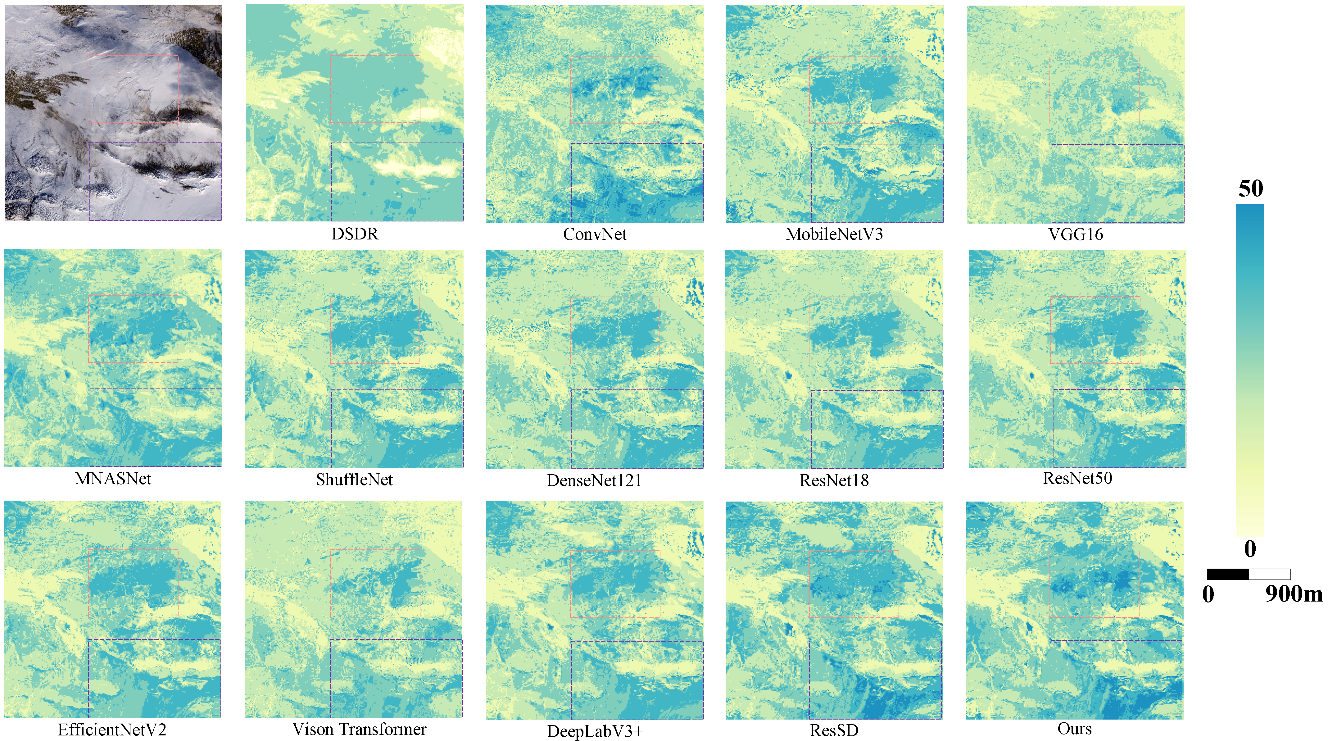
3.5.2. Visualizing Snow Depth Changes

For the time dimension, we also re-selected and downloaded two sets of multi-source snow remote sensing images of the TuoLi station in Xinjiang. As shown in Figure 12a,b, two sets of images show the snow depth of the TuoLi station area on 4 February 2015 and 27 February 2015, respectively, from left to right. Multi-spectral optical remote sensing data and corresponding snow depth maps are displayed. In order to clearly perceive the change in snow depth, we unified the snow depth gradient interval of 0∼45 cm. From the snow depth map, we can clearly see the change in snow cover in the whole area. Furthermore, in terms of details, based on the actual measurements from the meteorological stations over two days combined with the snow depth map, it can also be concluded that our method can effectively identify the accumulation trend of snow at TuoLi station. Hence, our method can be well applied to the snow depth mapping, effectively detecting different depths of snow and their changing trends.

4. Discussion

A series of experimental results demonstrate that our proposed deep learning method based on SAR remote sensing as a multi-source data input is feasible for estimating snow depth, achieving the best performance among all the metrics in the current research. In the ablation research section, data ablation shows that each data source is contributing to the final result in different ways, through model ablation, it shows that each module of MFPANet we proposed is effective, and they contribute to the realization of high-precision snow depth estimation. In the comparative study section, we show the improvement of our model in the field of snow depth estimation by comparing the relevant methods. It is worth mentioning that our model performs well in the estimation of shallow snow, and also shows excellent accuracy in the prediction of >30 cm deep snow, with RMSE of 0.474, with MAE of 0.221.

Table 7. The estimation results of our method on different snow depth ranges.

Snow Depth Range	RMSE	MAE
1–10 cm	0.118	0.043
10–20 cm	0.328	0.109
20–30 cm	0.423	0.167
>30 cm	0.479	0.198

shows the snow depth estimation result of our network in each depth interval. Due to the accumulation of snow cover, the snow layer of deep snow usually presents a multi-layer structure with instability, so deep snow is usually considered to be one of the potential hidden dangers of avalanches. The experiments have shown that our work on the accurate estimation of deep snow has a good application prospect in the prevention of avalanches and the avoidance of snow disasters.

On the other hand, compared to passive microwave remote sensing, which receives weak signals from the ground, SAR remote sensing actively generates signals and captures higher-quality echo signals for imaging. This results in a higher signal-to-noise ratio and provides high-quality, high-resolution remote sensing images for snow depth estimation studies. With the advancement of active microwave remote sensing technology and the deployment of multiple satellites, future snow depth estimation will benefit from even higher spatiotemporal resolution, helping to address various natural disasters and challenges more effectively.

4.1. Limitations

Although our snow depth estimation work has proposed MFPANet which is more suitable for the snow depth estimation task and shows better estimation accuracy than previous work, we should also recognize its limitations. At present, our proposed network cannot be well extended to other regions outside high-latitude regions of Asia. Because of the differences in altitude, annual average temperature, and snow media properties in different regions, the estimation of snow depth in different places is often ineffective. If there are enough local snow remote sensing data to support the training, our method can be extended to other regions, but for the time being, the lack of publicly available snow remote sensing datasets makes it difficult to achieve greater expansion and verification. Additionally, if the single pixel resolution of the satellite remote sensing used is high enough, then I think our method can be extended to provide higher resolution snow depth information.

4.2. Future Work

Although our current work has made progress in estimating snow depth in the high-latitude regions of Asia, and the proposed model shows decent predictive accuracy, looking ahead, with the continuous advancements and developments in radar and optical remote sensing technologies, our method holds significant potential for wider application and further exploration in both data and neural network methodologies. In terms of data, we can explore using remote sensing satellites or unmanned aerial vehicles (UAVs) with higher revisit frequencies and spatial resolutions. We could also consider employing polarimetric SAR with richer polarization modes or fully polarized SAR to acquire more precise ground station snow depth data. Additionally, fusing various auxiliary data sources such as temperature, elevation, and others is of great significance to promote snow depth estimation. In terms of the model, exploring more mainstream deep learning architectures or attention mechanisms could be beneficial. The continued exploration and adaptation of network structures suitable for snow depth estimation tasks could enable more accurate predictions of complex snow depths at higher spatial and temporal resolutions.

5. Conclusions

Achieving high-resolution snow depth estimation in high-latitude regions of Asia has always been an important issue. In order to solve this problem, we propose MFPANet, which is based on high-resolution multi-spectral optical remote sensing, SAR remote sensing and land cover data, and which relies on the measured snow depth data of ground meteorological stations. It shows unprecedented accuracy in snow depth prediction with a resolution of 320 m, with RMSE of 0.360, and with MAE of 0.128, $R^2$ reaches 0.997, which is of great value for hydrological simulation and regional snow disaster assessment in alpine regions. In addition, we use the residual network to build an MBFE unit, design modules such as MSFAA and HLF, mine semantic information at different scales, integrate features at different levels, and alleviate the complex ground object interference caused by spatial high resolution to snow depth estimation. Thus, a novel ‘area-to-point’ neural network suitable for snow depth estimation is obtained. Finally, our method can be used to generate high-resolution snow depth maps which play a role in hydrological simulation and snow disaster assessment. We hope that the proposed method can provide larger-scale, higher-resolution, and more accurate snow depth estimations for high-latitude regions of Asia, stimulate further research on snow depth estimation topics, and achieve comprehensive monitoring of the snow cryosphere. This is of great significance for solving the problem of more snow parameters in the cryosphere, and is crucial for the future of water resources management and sustainable development.

References

1. Estilow, T.W.; Young, A.H.; Robinson, D.A. A long-term Northern Hemisphere snow cover extent data record for climate studies and monitoring. Earth Syst. Sci. Data 2015, 7, 137–142. [Google Scholar] [CrossRef]
2. Che, T.; Dai, L.; Zheng, X.; Li, X.; Zhao, K. Estimation of snow depth from passive microwave brightness temperature data in forest regions of northeast China. Remote Sens. Environ. 2016, 183, 334–349. [Google Scholar] [CrossRef]
3. Kang, D.H.; Shi, X.; Gao, H.; Déry, S.J. On the changing contribution of snow to the hydrology of the Fraser River Basin, Canada. J. Hydrometeorol. 2014, 15, 1344–1365. [Google Scholar] [CrossRef]
4. Stott, P. How climate change affects extreme weather events. Science 2016, 352, 1517–1518. [Google Scholar] [CrossRef]
5. Tay, C.W.; Yun, S.H.; Chin, S.T.; Bhardwaj, A.; Jung, J.; Hill, E.M. Rapid flood and damage mapping using synthetic aperture radar in response to Typhoon Hagibis, Japan. Sci. Data 2020, 7, 100. [Google Scholar] [CrossRef]
6. Zhang, Y.; Liang, B. Evaluating the vulnerability of farming communities to winter storms in Iowa, US. Environ. Sustain. Indic. 2021, 11, 100126. [Google Scholar] [CrossRef]
7. Rumpf, S.B.; Gravey, M.; Brönnimann, O.; Luoto, M.; Cianfrani, C.; Mariethoz, G.; Guisan, A. From white to green: Snow cover loss and increased vegetation productivity in the European Alps. Science 2022, 376, 1119–1122. [Google Scholar] [CrossRef]
8. Gao, J.; Huang, X.; Ma, X.; Feng, Q.; Liang, T.; Xie, H. Snow disaster early warning in pastoral areas of Qinghai Province, China. Remote Sens. 2017, 9, 475. [Google Scholar] [CrossRef]
9. Bühler, Y.; Bebi, P.; Christen, M.; Margreth, S.; Stoffel, L.; Stoffel, A.; Marty, C.; Schmucki, G.; Caviezel, A.; Kühne, R.; et al. Automated avalanche hazard indication mapping on a statewide scale. Nat. Hazards Earth Syst. Sci. 2022, 22, 1825–1843. [Google Scholar] [CrossRef]
10. Rasmussen, R.; Baker, B.; Kochendorfer, J.; Meyers, T.; Landolt, S.; Fischer, A.P.; Black, J.; Thériault, J.M.; Kucera, P.; Gochis, D.; et al. How well are we measuring snow: The NOAA/FAA/NCAR winter precipitation test bed. Bull. Am. Meteorol. Soc. 2012, 93, 811–829. [Google Scholar] [CrossRef]
11. Hou, J.; Huang, C.; Zhang, Y.; Guo, J.; Gu, J. Gap-filling of MODIS fractional snow cover products via non-local spatio-temporal filtering based on machine learning techniques. Remote Sens. 2019, 11, 90. [Google Scholar] [CrossRef]
12. Wang, J.; Yuan, Q.; Shen, H.; Liu, T.; Li, T.; Yue, L.; Shi, X.; Zhang, L. Estimating snow depth by combining satellite data and ground-based observations over Alaska: A deep learning approach. J. Hydrol. 2020, 585, 124828. [Google Scholar] [CrossRef]
13. Xing, D.; Hou, J.; Huang, C.; Zhang, W. Estimation of Snow Depth from AMSR2 and MODIS Data based on Deep Residual Learning Network. Remote Sens. 2022, 14, 5089. [Google Scholar] [CrossRef]
14. Daudt, R.C.; Wulf, H.; Hafner, E.D.; Bühler, Y.; Schindler, K.; Wegner, J.D. Snow depth estimation at country-scale with high spatial and temporal resolution. ISPRS J. Photogramm. Remote Sens. 2023, 197, 105–121. [Google Scholar] [CrossRef]
15. Kelly, R.E.; Chang, A.T.; Tsang, L.; Foster, J.L. A prototype AMSR-E global snow area and snow depth algorithm. IEEE Trans. Geosci. Remote Sens. 2003, 41, 230–242. [Google Scholar] [CrossRef]
16. Olefs, M.; Koch, R.; Schöner, W.; Marke, T. Changes in snow depth, snow cover duration, and potential snowmaking conditions in Austria, 1961–2020—A model based approach. Atmosphere 2020, 11, 1330. [Google Scholar] [CrossRef]
17. Zhu, L.; Zhang, Y.; Wang, J.; Tian, W.; Liu, Q.; Ma, G.; Kan, X.; Chu, Y. Downscaling snow depth mapping by fusion of microwave and optical remote-sensing data based on deep learning. Remote Sens. 2021, 13, 584. [Google Scholar] [CrossRef]
18. Patil, A.; Singh, G.; Rüdiger, C. Retrieval of snow depth and snow water equivalent using dual polarization SAR data. Remote Sens. 2020, 12, 1183. [Google Scholar] [CrossRef]
19. Qiao, H.; Zhang, P.; Li, Z.; Huang, L.; Gao, S.; Liu, C.; Wu, Z.; Liang, S.; Zhou, J.; Sun, W.; et al. A new snow depth retrieval method by improved hybrid DEM differencing and coherence amplitude algorithm for PolInSAR. J. Hydrol. 2024, 628, 130507. [Google Scholar]
20. Shi, J.; Dozier, J. Estimation of snow water equivalence using SIR-C/X-SAR. II. Inferring snow depth and particle size. IEEE Trans. Geosci. Remote Sens. 2000, 38, 2475–2488. [Google Scholar]
21. Leinss, S.; Parrella, G.; Hajnsek, I. Snow height determination by polarimetric phase differences in X-band SAR data. IEEE J. Sel. Top. Appl. Earth Obs. Remote Sens. 2014, 7, 3794–3810. [Google Scholar] [CrossRef]
22. Leinss, S.; Löwe, H.; Proksch, M.; Lemmetyinen, J.; Wiesmann, A.; Hajnsek, I. Anisotropy of seasonal snow measured by polarimetric phase differences in radar time series. Cryosphere 2016, 10, 1771–1797. [Google Scholar] [CrossRef]
23. Evans, J.R.; Kruse, F.A. Determination of snow depth using elevation differences determined by interferometric SAR (InSAR). In Proceedings of the 2014 IEEE Geoscience and Remote Sensing Symposium, Quebec City, QC, Canada, 13–18 July2014; pp. 962–965. [Google Scholar]
24. Li, H.; Xiao, P.; Feng, X.; He, G.; Wang, Z. Monitoring snow depth and its change using repeat-pass interferometric SAR in Manas River Basin. In Proceedings of the 2016 IEEE International Geoscience and Remote Sensing Symposium (IGARSS), Beijing, China, 10–15 July 2016; pp. 4936–4939. [Google Scholar]
25. Yang, J.; Li, C. Assimilation of D-InSAR snow depth data by an ensemble Kalman filter. Arab. J. Geosci. 2021, 14, 505. [Google Scholar] [CrossRef]
26. Lievens, H.; Demuzere, M.; Marshall, H.P.; Reichle, R.H.; Brucker, L.; Brangers, I.; de Rosnay, P.; Dumont, M.; Girotto, M.; Immerzeel, W.W.; et al. Snow depth variability in the Northern Hemisphere mountains observed from space. Nat. Commun. 2019, 10, 4629. [Google Scholar] [CrossRef]
27. Yin, H.; Weng, L.; Li, Y.; Xia, M.; Hu, K.; Lin, H.; Qian, M. Attention-guided siamese networks for change detection in high resolution remote sensing images. Int. J. Appl. Earth Obs. Geoinf. 2023, 117, 103206. [Google Scholar] [CrossRef]
28. Song, L.; Xia, M.; Weng, L.; Lin, H.; Qian, M.; Chen, B. Axial cross attention meets CNN: Bibranch fusion network for change detection. IEEE J. Sel. Top. Appl. Earth Obs. Remote Sens. 2022, 16, 32–43. [Google Scholar] [CrossRef]
29. Ren, H.; Xia, M.; Weng, L.; Hu, K.; Lin, H. Dual-Attention-Guided Multiscale Feature Aggregation Network for Remote Sensing Image Change Detection. IEEE J. Sel. Top. Appl. Earth Obs. Remote Sens. 2024, 17, 4899–4916. [Google Scholar] [CrossRef]
30. Wang, Z.; Xia, M.; Weng, L.; Hu, K.; Lin, H. Dual Encoder–Decoder Network for Land Cover Segmentation of Remote Sensing Image. IEEE J. Sel. Top. Appl. Earth Obs. Remote Sens. 2024, 17, 2372–2385. [Google Scholar] [CrossRef]
31. Yu, X.; Hu, X.; Wang, G.; Wang, K.; Chen, X. Machine-Learning Estimation of Snow Depth in 2021 Texas Statewide Winter Storm Using SAR Imagery. Geophys. Res. Lett. 2022, 49, e2022GL099119. [Google Scholar] [CrossRef]
32. Varade, D.; Manickam, S.; Dikshit, O.; Singh, G. Modelling of early winter snow density using fully polarimetric c-band sar data in the indian himalayas. Remote Sens. Environ. 2020, 240, 111699. [Google Scholar] [CrossRef]
33. Singh, G.; Venkataraman, G. Algorithm development for snow density estimation using polarimetric advanced SAR data. In Remote Sensing for Agriculture, Ecosystems, and Hydrology XI; SPIE: San Diego, CA, USA, 2009; pp. 202–208. [Google Scholar]
34. He, K.; Zhang, X.; Ren, S.; Sun, J. Deep residual learning for image recognition. In Proceedings of the IEEE Conference on Computer Vision and Pattern Recognition, Las Vegas, NV, USA, 26 June–1 July 2016; pp. 770–778. [Google Scholar]
35. Zhao, H.; Shi, J.; Qi, X.; Wang, X.; Jia, J. Pyramid scene parsing network. In Proceedings of the IEEE Conference on Computer Vision and Pattern Recognition, Honolulu, HI, USA, 21–26 July 2017; pp. 2881–2890. [Google Scholar]
36. Dai, X.; Xia, M.; Weng, L.; Hu, K.; Lin, H.; Qian, M. Multi-Scale Location Attention Network for Building and Water Segmentation of Remote Sensing Image. IEEE Trans. Geosci. Remote Sens. 2023, 61, 5609519. [Google Scholar] [CrossRef]
37. Chen, K.; Xia, M.; Lin, H.; Qian, M. Multi-scale Attention Feature Aggregation Network for Cloud and Cloud Shadow Segmentation. IEEE Trans. Geosci. Remote Sens. 2023, 61, 5612216. [Google Scholar]
38. Ulaby, F.T.; Stiles, W.H.; AbdelRazik, M. Snowcover influence on backscattering from terrain. IEEE Trans. Geosci. Remote Sens. 1984, GE-22, 126–133. [Google Scholar]
39. Yao, H.; Zhang, Y.; Jiang, L.; Ewe, H.T.; Ng, M. Snow Parameters Inversion from Passive Microwave Remote Sensing Measurements by Deep Convolutional Neural Networks. Sensors 2022, 22, 4769. [Google Scholar] [CrossRef]
40. Simonyan, K.; Zisserman, A. Very deep convolutional networks for large-scale image recognition. arXiv 2014, arXiv:1409.1556. [Google Scholar]
41. Howard, A.; Sandler, M.; Chu, G.; Chen, L.C.; Chen, B.; Tan, M.; Wang, W.; Zhu, Y.; Pang, R.; Vasudevan, V.; et al. Searching for mobilenetv3. In Proceedings of the IEEE/CVF International Conference on Computer Vision, Seoul, Republic of Korea, 27 October–2 November 2019; pp. 1314–1324. [Google Scholar]
42. Ma, N.; Zhang, X.; Zheng, H.T.; Sun, J. Shufflenet v2: Practical guidelines for efficient cnn architecture design. In Proceedings of the European Conference on Computer Vision (ECCV), Munich, Germany, 8–14 September 2018; pp. 116–131. [Google Scholar]
43. Huang, G.; Liu, Z.; Van Der Maaten, L.; Weinberger, K.Q. Densely connected convolutional networks. In Proceedings of the IEEE Conference on Computer Vision and Pattern Recognition, Honolulu, HI, USA, 21–26 July 2017; pp. 4700–4708. [Google Scholar]
44. Tan, M.; Chen, B.; Pang, R.; Vasudevan, V.; Sandler, M.; Howard, A.; Le, Q.V. Mnasnet: Platform-aware neural architecture search for mobile. In Proceedings of the IEEE/CVF Conference on Computer Vision and Pattern Recognition, Long Beach, CA, USA, 15–20 June 2019; pp. 2820–2828. [Google Scholar]
45. Tan, M.; Le, Q. Efficientnet: Rethinking model scaling for convolutional neural networks. In Proceedings of the International Conference on Machine Learning, PMLR, Long Beach, CA, USA, 9–15 June 2019; pp. 6105–6114. [Google Scholar]
46. Vaswani, A.; Shazeer, N.; Parmar, N.; Uszkoreit, J.; Jones, L.; Gomez, A.N.; Kaiser, Ł.; Polosukhin, I. Attention is all you need. In Proceedings of the Advances in Neural Information Processing Systems 30 (NIPS 2017), Long Beach, CA, USA, 4–9 December 2017. [Google Scholar]
47. Chen, L.C.; Zhu, Y.; Papandreou, G.; Schroff, F.; Adam, H. Encoder-decoder with atrous separable convolution for semantic image segmentation. In Proceedings of the European Conference on Computer Vision (ECCV), Munich, Germany, 8–14 September 2018; pp. 801–818. [Google Scholar]
Figure 1. Framework of multi-scale feature perception and aggregation network.
Remotesensing 16 02087 g001
Figure 2. The structure of the residual layer in MBFE, (a) represents the internal structure of the residual layer without the downsampling operation, (b) represents the internal structure of the residual layer with the downsampling operation. f denotes the input of the residual layer, and  f  denotes the output of the residual layers.
Remotesensing 16 02087 g002
Figure 3. The structure of the MSFAA module. f denotes the input of the module,  f  denotes the output of the module.
Remotesensing 16 02087 g003
Figure 4. The structure of the HLF module.
Remotesensing 16 02087 g004
Figure 5. Location of the study area, including the Qinghai–Tibet Plateau, Xinjiang and Gansu province. The figure shows the elevation information of our study area, and the red marker is the meteorological station involved in the dataset we collected.
Remotesensing 16 02087 g005
Figure 6. Data distribution of our SRSD dataset. It is an eight-channel snow remote sensing dataset that fuses multi-source remote sensing data, including snow depth labels corresponding to 0∼42 cm.
Remotesensing 16 02087 g006
Figure 7. Multi-source data selection of this work; we randomly cropped and selected a set of data sources for display. The image on the left is a multi-spectral optical remote sensing image, the middle image is a VV single-polarization Sentinel-1 SAR image, and the image on the right displays corresponding land cover data.
Remotesensing 16 02087 g007
Figure 8. A 2D scatter diagram of measured snow depth values versus estimated by different data combinations using our method, where the green line is y = x line. The 4 channels represent the data combination of SAR + land cover, 5 channels represent the data combination of SAR + multi-spectral optical, 7 channels represent the data combination of multi-spectral optical + land cover, and our 8 channels’ data combination strategy (multi-spectral optical + SAR + Land cover) has better fitting ability by our method.
Remotesensing 16 02087 g008
Figure 9. A 2D scatter diagram of the measured snow depth values versus those estimated by different deep learning methods in the comparable studies section, which include existing snow depth estimation methods and excellent methods in image classification or image segmentation. The accuracy of snow depth estimation is also shown on the scatter plots of each method. The green line is y = x line. It is obvious that our method has better fitting ability.
Remotesensing 16 02087 g009
Figure 10. Snow depth mapping by different methods in the comparable studies section. We used purple and red matrix boxes to mark the parts with large differences in snow depth distributions in each model. We unified the snow depth scale in 0∼50 cm to observe the snow depth estimation ability of different models. According to the boxed area, we can find that the model has problems in a wide range of generalization applications when it performs similarly on our dataset; it may not be able to predict deep snow well, or it may not fit the terrain distribution well. In contrast, our proposed network can better fit terrain features and better estimate deep snow.
Remotesensing 16 02087 g010
Figure 11. Snow depth mapping by our method. (a,b) Two sets of snow depth maps show the estimation effect of our method on >30 cm deep snow through local amplification of the station. (c,d) Two sets of snow depth maps show the estimation effect of our method on <30 cm light snow through local amplification of the station, and the pink circle represents the location of the station. The red value denotes the measured snow depth value of the station on the day.
Remotesensing 16 02087 g011
Figure 12. Snow depth mapping by our method. (a,b) Two sets of images in this figure show the snow depth of TuoLi station area on 4 February 2015 and 27 February 2015. We can infer from the diagram that our method can perceive the changing trend in snow cover well.
Remotesensing 16 02087 g012