
Comparison of Machine Learning Models in Simulating Glacier Mass Balance: Insights from Maritime and Continental Glaciers in High Mountain Asia
 , , , , and
Abstract
:
1. Introduction
2. Study Area and Data
2.1. Study Area
2.2. Data
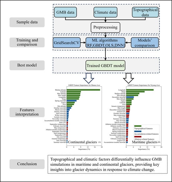
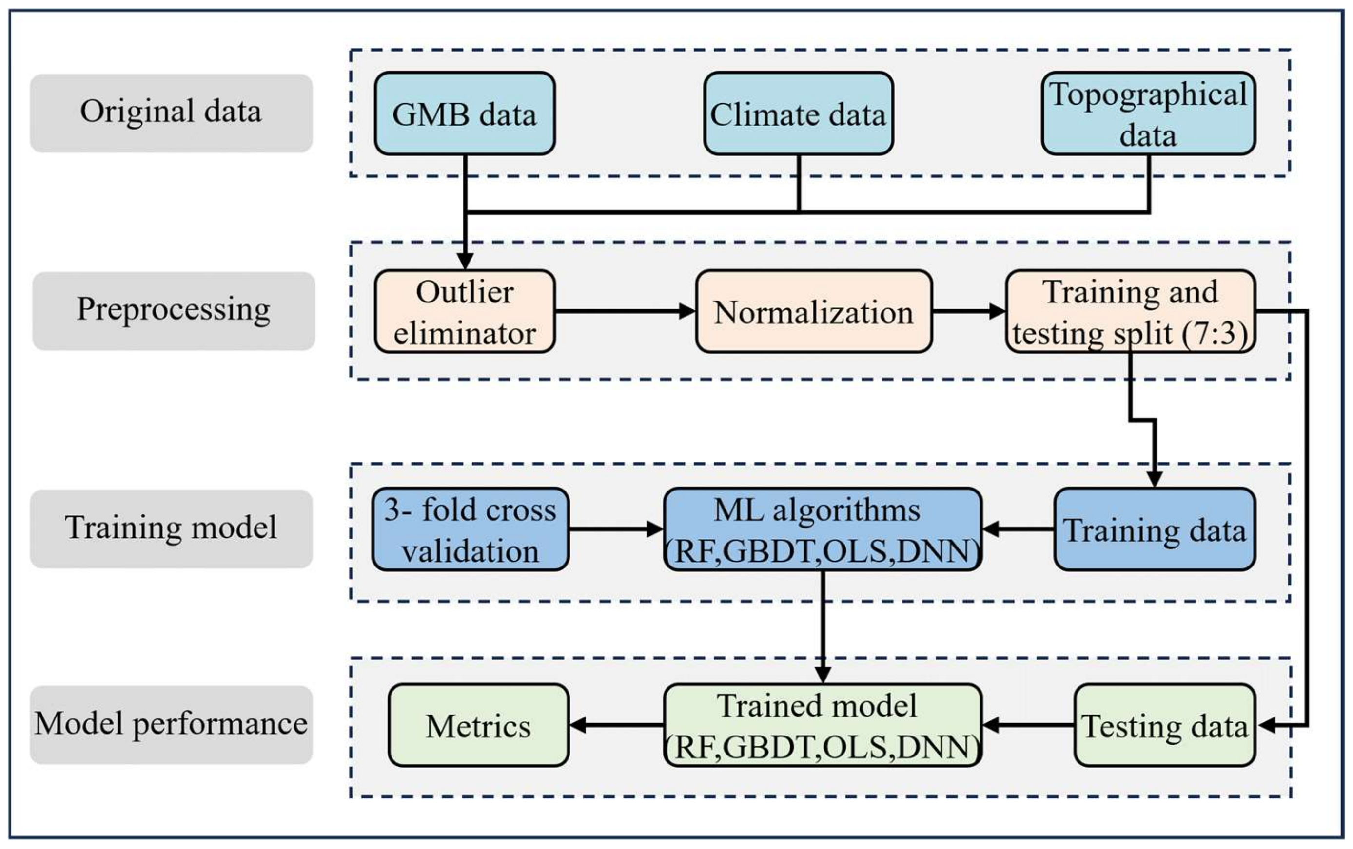
3. Methodology
3.1. Machine Learning Algorithms
3.1.1. Random Forest Models
3.1.2. Gradient Boosting Decision Tree
3.1.3. Deep Neural Network
3.2. Performance Measures
3.3. Hyperparameter Selection
4. Results
4.1. Selection of Predictors
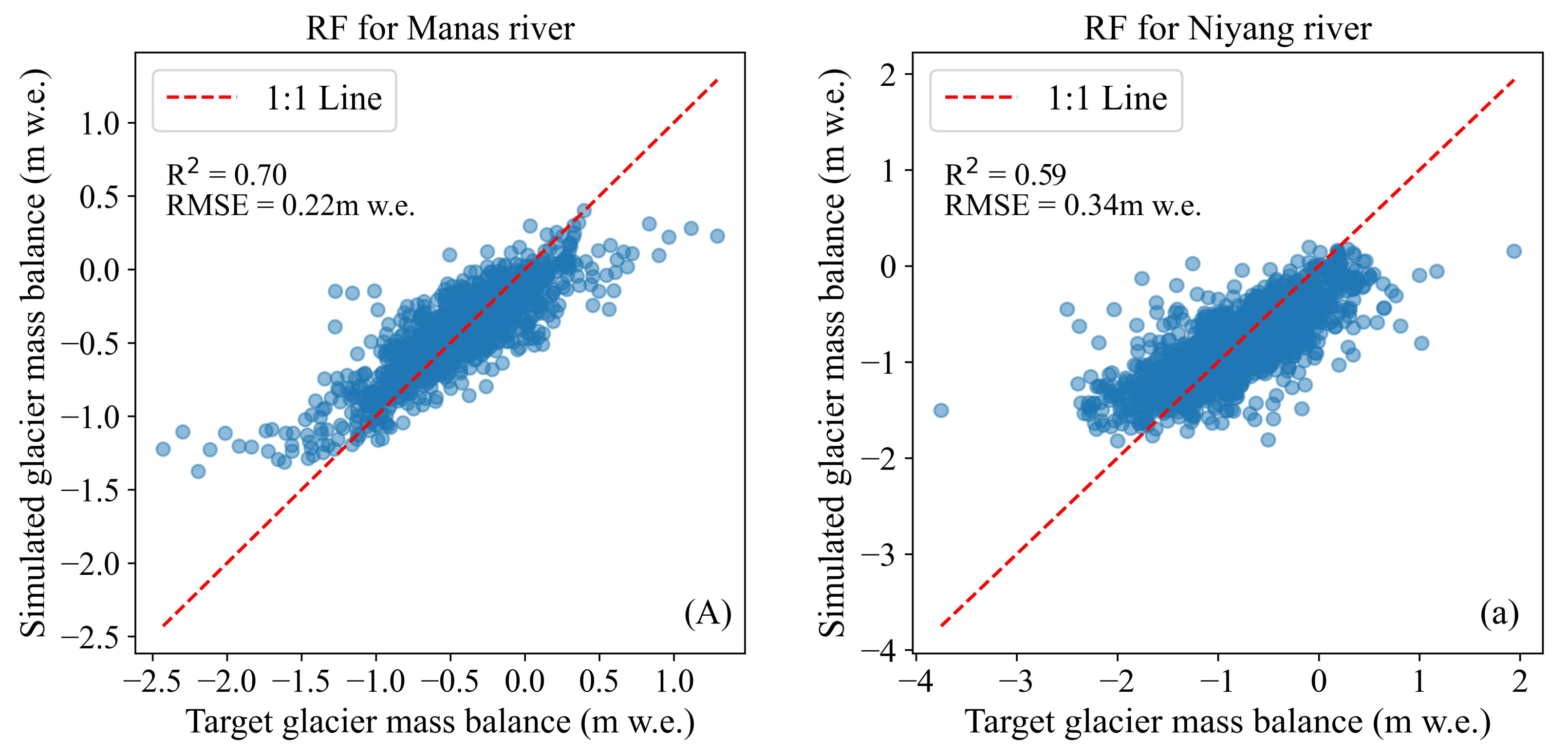
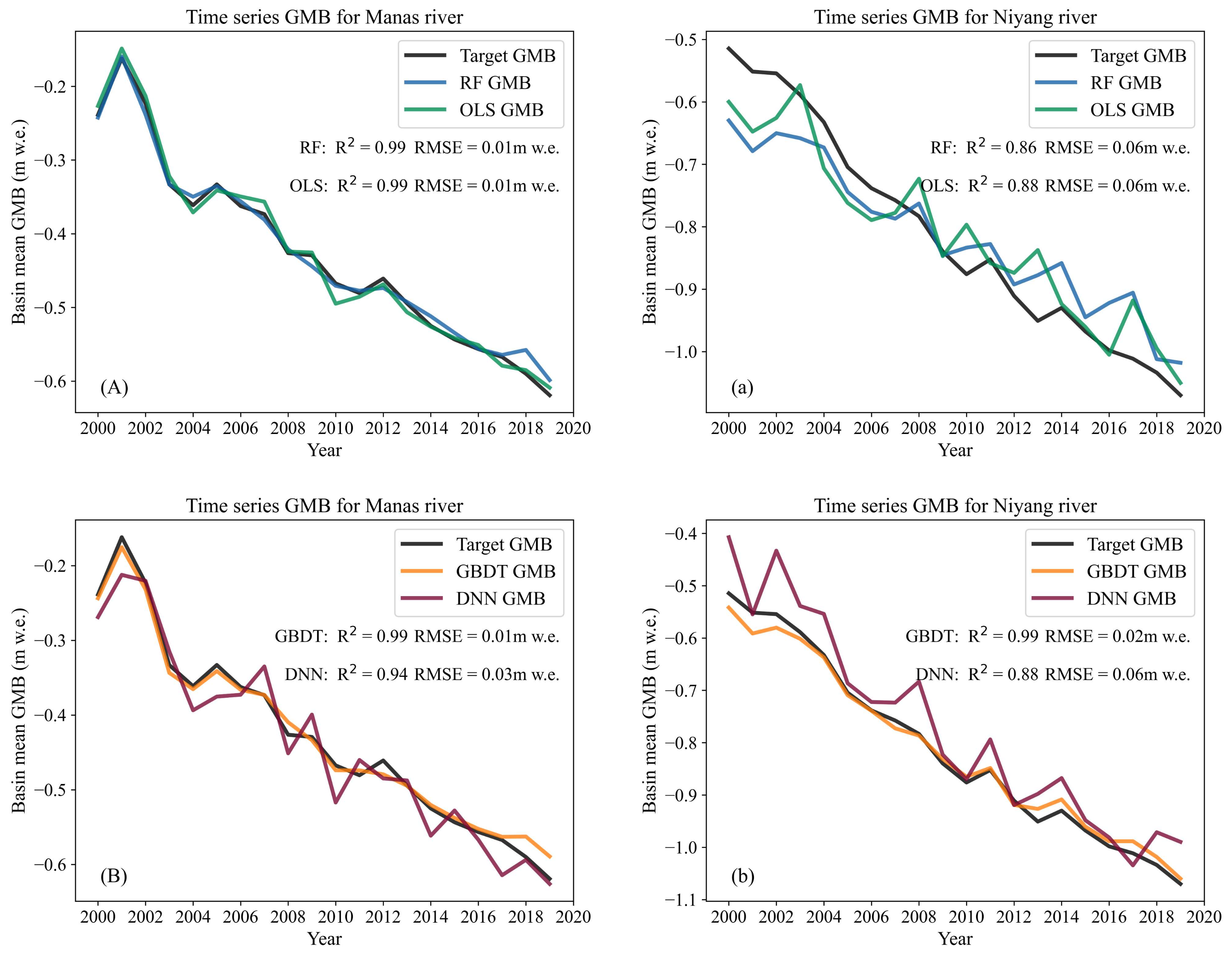
4.2. Overall Performance of the Four ML Models
4.3. Basin Analysis
5. Discussion
5.1. The Influence of Outliers
5.2. The Potential of Temporal Predictive Models
5.3. Limitations of the Current Study
6. Conclusions
Author Contributions
Funding
Data Availability Statement
Acknowledgments
Conflicts of Interest
References
- Biemans, H.; Siderius, C.; Lutz, A.F.; Nepal, S.; Ahmad, B.; Hassan, T. Importance of snow and glacier meltwater for agriculture on the Indo-Gangetic Plain. Nat. Sustain. 2019, 2, 594–601. [Google Scholar] [CrossRef]
- Immerzeel, W.W.; Lutz, A.F.; Andrade, M.; Bahl, A.; Biemans, H.; Bolch, T.; Hyde, S.; Brumby, S.; Davies, B.J.; Elmore, A.C.; et al. Importance and vulnerability of the world’s water towers. Nature 2020, 577, 364–369. [Google Scholar] [CrossRef]
- Miles, E.; McCarthy, M.; Dehecq, A.; Kneib, M.; Fugger, S.; Pellicciotti, F. Health and sustainability of glaciers in High Mountain Asia. Nat. Commun. 2021, 12, 2868. [Google Scholar] [CrossRef]
- Marzeion, B.; Hock, R.; Anderson, B.; Bliss, A.; Champollion, N.; Fujita, K.; Huss, M.; Immerzeel, W.W.; Kraaijenbrink, P.; Malles, J.H.; et al. Partitioning the uncertainty of ensemble projections of global glacier mass change. Earth’s Future 2020, 8, e2019EF001470. [Google Scholar] [CrossRef]
- Zemp, M.; Huss, M.; Thibert, E.; Eckert, N.; McNabb, R.; Huber, J.; Barandun, M.; Machguth, H.; Nussbaumer, S.U.; Gärtner-Roer, I.; et al. Global glacier mass changes and their contributions to sea-level rise from 1961 to 2016. Nature 2019, 568, 382–386. [Google Scholar] [CrossRef]
- Huss, M.; Hock, R. Global-scale hydrological response to future glacier mass loss. Nat. Clim. Chang. 2018, 8, 135–140. [Google Scholar] [CrossRef]
- Li, X.; Cheng, G.; Fu, B.; Xia, J.; Zhang, L.; Yang, D.; Zheng, C.; Liu, S.; Li, X.; Song, C.; et al. Linking critical zone with watershed science: The example of the Heihe River basin. Earth’s Future 2022, 10, e2022EF002966. [Google Scholar] [CrossRef]
- Li, X.; Feng, M.; Ran, Y.; Su, Y.; Liu, F.; Huang, C.; Shen, H.; Xiao, Q.; Su, J.; Yuan, S.; et al. Big Data in Earth system science and progress towards a digital twin. Nat. Rev. Earth Environ. 2023, 4, 319–332. [Google Scholar] [CrossRef]
- Zeng, R.; Ren, W. The spatiotemporal trajectory of US agricultural irrigation withdrawal during 1981–2015. Environ. Res. Lett 2022, 17, 104027. [Google Scholar] [CrossRef]
- Ren, W.; Li, X.; Zheng, D.; Zeng, R.; Su, J.; Mu, T.; Wang, Y. Enhancing Flood Simulation in Data-Limited Glacial River Basins through Hybrid Modeling and Multi-Source Remote Sensing Data. Remote Sens. 2023, 15, 4527. [Google Scholar] [CrossRef]
- Liu, H.; Wang, L.; Zhou, J.; Shrestha, M.; Chai, C.; Li, X.; Ahmad, B. Energy-balance modeling of heterogeneous glacio-hydrological regimes at upper Indus. J. Hydrol. Reg. Stud. 2023, 49, 101515. [Google Scholar] [CrossRef]
- Ismail, M.F.; Bogacki, W.; Disse, M.; Schäfer, M.; Kirschbauer, L. Estimating degree-day factors of snow based on energy flux components. Cryosphere 2023, 17, 211–231. [Google Scholar] [CrossRef]
- Ren, W.; Yang, T.; Shi, P.; Xu, C.Y.; Zhang, K.; Zhou, X.; Shao, Q.; Ciais, P. A probabilistic method for streamflow projection and associated uncertainty analysis in a data sparse alpine region. Glob. Planet. Chang. 2018, 165, 100–113. [Google Scholar] [CrossRef]
- Lutz, A.F.; Immerzeel, W.W.; Shrestha, A.B.; Bierkens, M.F.P. Consistent increase in High Asia’s runoff due to increasing glacier melt and precipitation. Nat. Clim. Chang. 2014, 4, 587–592. [Google Scholar] [CrossRef]
- Khanal, S.; Lutz, A.F.; Kraaijenbrink, P.D.A.; Hurk, B.v.D.; Yao, T.; Immerzeel, W.W. Variable 21st century climate change response for rivers in High Mountain Asia at seasonal to decadal time scales. Water Resour. Res. 2021, 57, e2020WR029266. [Google Scholar] [CrossRef]
- Gao, R.; Torres-Rua, A.F.; Aboutalebi, M.; White, W.A.; Anderson, M.; Kustas, W.P.; Agam, N.; Alsina, M.M.; Alfieri, J.; Hipps, L.; et al. LAI estimation across California vineyards using sUAS multi-seasonal multi-spectral, thermal, and elevation information and machine learning. Irrig. Sci. 2022, 40, 731–759. [Google Scholar] [CrossRef]
- Ren, W.W.; Yang, T.; Huang, C.S.; Xu, C.Y.; Shao, Q.X. Improving monthly streamflow prediction in alpine regions: Integrating HBV model with Bayesian neural network. Stoch. Environ. Res. Risk Assess. 2018, 32, 3381–3396. [Google Scholar] [CrossRef]
- Hugonnet, R.; McNabb, R.; Berthier, E.; Menounos, B.; Nuth, C.; Girod, L.; Farinotti, D.; Huss, M.; Dussaillant, I.; Brun, F.; et al. Accelerated global glacier mass loss in the early twenty-first century. Nature 2021, 592, 726–731. [Google Scholar] [CrossRef] [PubMed]
- Hoinkes, H.C. Glacier variation and weather. J. Glaciol. 1968, 7, 3–18. [Google Scholar] [CrossRef]
- Bolibar, J.; Rabatel, A.; Gouttevin, I.; Galiez, C.; Condom, T.; Sauquet, E. Deep learning applied to glacier evolution modelling. Cryosphere 2020, 14, 565–584. [Google Scholar] [CrossRef]
- Anilkumar, R.; Bharti, R.; Chutia, D.; Aggarwal, S.P. Modelling point mass balance for the glaciers of the Central European Alps using machine learning techniques. Cryosphere 2023, 17, 2811–2828. [Google Scholar] [CrossRef]
- Brun, F.; Berthier, E.; Wagnon, P.; Kääb, A.; Treichler, D. A spatially resolved estimate of High Mountain Asia glacier mass balances from 2000 to 2016. Nat. Geosci. 2017, 10, 668–673. [Google Scholar] [CrossRef]
- Zhao, F.; Long, D.; Li, X.; Huang, Q.; Han, P. Rapid glacier mass loss in the Southeastern Tibetan Plateau since the year 2000 from satellite observations. Remote Sens. Environ. 2022, 270, 112853. [Google Scholar] [CrossRef]
- Zhang, Z.; Gu, Z.; Hu, K.; Xu, Y.; Zhao, J. Spatial variability between glacier mass balance and environmental factors in the High Mountain Asia. J. Arid. Land 2022, 14, 441–454. [Google Scholar] [CrossRef]
- Kraaijenbrink, P.D.; Bierkens, M.F.; Lutz, A.F.; Immerzeel, W.W. Impact of a global temperature rise of 1.5 degrees Celsius on Asia’s glaciers. Nature 2017, 549, 257–260. [Google Scholar] [CrossRef]
- Yao, T.; Thompson, L.; Yang, W.; Yu, W.; Gao, Y.; Guo, X.; Yang, X.; Duan, K.; Zhao, H.; Xu, B.; et al. Different glacier status with atmospheric circulations in Tibetan Plateau and surroundings. Nat. Clim. Chang. 2012, 2, 663–667. [Google Scholar] [CrossRef]
- Fujita, K. Influence of precipitation seasonality on glacier mass balance and its sensitivity to climate change. Ann. Glaciol. 2008, 48, 88–92. [Google Scholar] [CrossRef]
- Yao, T.D.; Yu, W.S.; Wu, G.J.; Xu, B.; Yang, W.; Zhao, H.; Wang, W.; Li, S.; Wang, N.; Li, Z.; et al. Glacier anomalies and relevant disaster risks on the Tibetan Plateau and surroundings. Chin. Sci. Bull. 2019, 64, 2770–2782. (In Chinese) [Google Scholar]
- Muñoz-Sabater, J.; Dutra, E.; Agustí-Panareda, A.; Albergel, C.; Arduini, G.; Balsamo, G.; Boussetta, S.; Choulga, M.; Harrigan, S.; Hersbach, H.; et al. ERA5-Land: A state-of-the-art global reanalysis dataset for land applications. Earth Syst. Sci. Data 2021, 13, 4349–4383. [Google Scholar] [CrossRef]
- RGI Consortium. GLIMS: Global Land Ice Measurements from Space, A Dataset of Global Glacier Outlines Version 6.0 Technical Report, Colorado, USA. 2017. Available online: https://www.glims.org/RGI/randolph60.html (accessed on 10 January 2024).
- Zhang, Z.; Li, Z.; He, X. Progress in the research on glacial change and water resources in Manas river basin. Int. Soil Water Conserv. Res. 2014, 25, 332–337. (In Chinese) [Google Scholar]
- Wang, X.; Yang, T.; Xu, C.Y.; Yong, B.; Shi, P. Understanding the discharge regime of a glacierized alpine catchment in the Tianshan Mountains using an improved HBV-D hydrological model. Glob. Planet. Chang. 2019, 172, 211–222. [Google Scholar] [CrossRef]
- Ji, X.; Chen, Y. Characterizing spatial patterns of precipitation based on corrected TRMM 3B43 data over the mid Tianshan Mountains of China. J. Mt. Sci. 2012, 9, 628–645. [Google Scholar] [CrossRef]
- Zhang, M.; Ren, Q.; Wei, X.; Wang, J.; Yang, X.; Jiang, Z. Climate change, glacier melting and streamflow in the Niyang River Basin, Southeast Tibet, China. Ecohydrology 2011, 4, 288–298. [Google Scholar] [CrossRef]
- Wu, X.; Su, J.; Ren, W.; Lü, H.; Yuan, F. Statistical comparison and hydrological utility evaluation of ERA5-Land and IMERG precipitation products on the Tibetan Plateau. J. Hydrol. 2023, 620, 129384. [Google Scholar] [CrossRef]
- Yilmaz, M. Accuracy assessment of temperature trends from ERA5 and ERA5-Land. Sci. Total Environ. 2023, 856, 159182. [Google Scholar] [CrossRef] [PubMed]
- Zhou, L.; Pan, S.; Wang, J.; Vasilakos, A.V. Machine learning on big data: Opportunities and challenges. Neurocomputing 2017, 237, 350–361. [Google Scholar] [CrossRef]
- Schoppa, L.; Disse, M.; Bachmair, S. Evaluating the performance of random forest for large-scale flood discharge simulation. J. Hydrol. 2020, 590, 125531. [Google Scholar] [CrossRef]
- Rahman, A.; Hosono, T.; Quilty, J.M.; Das, J.; Basak, A. Multiscale groundwater level forecasting: Coupling new machine learning approaches with wavelet transforms. Adv. Water Resour. 2020, 141, 103595. [Google Scholar] [CrossRef]
- Seydi, S.T.; Kanani-Sadat, Y.; Hasanlou, M.; Sahraei, R.; Chanussot, J.; Amani, M. Comparison of machine learning algorithms for flood susceptibility mapping. Remote Sens. 2022, 15, 192. [Google Scholar] [CrossRef]
- He, X.; Luo, J.; Zuo, G.; Xie, J. Daily runoff forecasting using a hybrid model based on variational mode decomposition and deep neural networks. Water Resour. Manag. 2019, 33, 1571–1590. [Google Scholar] [CrossRef]
- Kadow, C.; Hall, D.M.; Ulbrich, U. Artificial intelligence reconstructs missing climate information. Nat. Geosci. 2020, 13, 408–413. [Google Scholar] [CrossRef]
- Bolibar, J.; Rabatel, A.; Gouttevin, I.; Zekollari, H.; Galiez, C. Nonlinear sensitivity of glacier mass balance to future climate change unveiled by deep learning. Nat. Commun. 2022, 13, 409. [Google Scholar] [CrossRef]
- Pedregosa, F.; Varoquaux, G.; Gramfort, A.; Michel, V.; Thirion, B.; Grisel, O.; Blondel, M.; Prettenhofer, P.; Weiss, R.; Dubourg, V.; et al. Scikit-learn: Machine learning in Python. J. Mach. Learn. Res. 2011, 12, 2825–2830. [Google Scholar]
- Brun, F.; Wagnon, P.; Berthier, E.; Jomelli, V.; Maharjan, S.B.; Shrestha, F.; Kraaijenbrink, P.D.A. Heterogeneous influence of glacier morphology on the mass balance variability in High Mountain Asia. J. Geophys. Res. Earth Surf. 2019, 124, 1331–1345. [Google Scholar] [CrossRef]
- Rabatel, A.; Dedieu, J.P.; Vincent, C. Spatio-temporal changes in glacier-wide mass balance quantified by optical remote sensing on 30 glaciers in the French Alps for the period 1983–2014. J. Glaciol. 2016, 62, 1153–1166. [Google Scholar] [CrossRef]
- Braithwaite, R.J.; Raper, S.C.B. Estimating equilibrium-line altitude (ELA) from glacier inventory data. Ann. Glaciol. 2009, 50, 127–132. [Google Scholar] [CrossRef]
- Maurer, J.M.; Schaefer, J.M.; Rupper, S.; Corley, A.J.S.A. Acceleration of ice loss across the Himalayas over the past 40 years. Sci. Adv. 2019, 5, eaav7266. [Google Scholar] [CrossRef]
- Liang, L.; Cuo, L.; Liu, Q. Mass balance variation and associative climate drivers for the Dongkemadi Glacier in the central Tibetan Plateau. J. Geophys. Res. Atmos. 2019, 124, 10814–10825. [Google Scholar] [CrossRef]
- Rani, S.; Mal, S. Trends in land surface temperature and its drivers over the High Mountain Asia. Egypt. J. Remote Sens. Space Sci. 2022, 25, 717–729. [Google Scholar] [CrossRef]
- He, Q.; Kuang, X.; Chen, J.; Feng, Y.; Zheng, C. Reconstructing runoff components and glacier mass balance with climate change: Niyang River basin, southeastern Tibetan Plateau. Front. Earth Sci. 2023, 11, 1165390. [Google Scholar] [CrossRef]
- Xiao, Y.; Ke, C.Q.; Shen, X.; Cai, Y.; Li, H. What drives the decrease of glacier surface albedo in High Mountain Asia in the past two decades? Sci. Total Environ. 2023, 863, 160945. [Google Scholar] [CrossRef] [PubMed]
- Zhang, Y.; Kang, S.; Cong, Z.; Schmale, J.; Sprenger, M.; Li, C.; Yang, W.; Gao, T.; Sillanpää, M.; Li, X.; et al. Light-absorbing impurities enhance glacier albedo reduction in the southeastern Tibetan Plateau. J. Geophys. Res. Atmos. 2017, 122, 6915–6933. [Google Scholar] [CrossRef]
- Zhao, P.; He, Z. A first evaluation of ERA5-Land reanalysis temperature product over the Chinese Qilian Mountains. Front. Earth Sci. 2022, 10, 907730. [Google Scholar] [CrossRef]


| Algorithm | Hyperparameter | Value for MRB | Value for NRB |
|---|---|---|---|
| RF | Number of trees | 100 | 120 |
| Maximum number of features | 4 | 5 | |
| Minimum split samples | 5 | 8 | |
| Maximum depth | None | None | |
| Minimum samples of leaf nodes | 4 | 6 | |
| DNN | Learning rate | 0.001 | 0.001 |
| Epochs | 1000 | 2000 | |
| Hidden layers | 20 | 20 | |
| Activation function | ReLu | ReLu | |
| GBDT | Learning rate | 0.01 | 0.1 |
| Number of trees | 450 | 250 | |
| Maximum number of features | 3 | 3 | |
| Minimum split samples | 5 | 4 | |
| Maximum depth | 8 | 8 | |
| Minimum samples of leaf nodes | 2 | 1 |
| Topographical Variables | Ablation-Related Variables | Accumulation-Related Variables | |
|---|---|---|---|
| Longitude | Annual CPT | Monthly accumulation temperature | Annual snowfall |
| Latitude | Monthly ablation CPT | Spring temperature | Monthly ablation snowfall |
| Median altitude | Monthly accumulation CPT | Summer temperature | Monthly accumulation snowfall |
| Min altitude | Spring CPT | Autumn temperature | Spring snowfall |
| Max altitude | Summer CPT | Winter temperature | Summer snowfall |
| Slope | Autumn CPT | 1~12 temperature | Autumn snowfall |
| Aspect | 4~10 CPT | Winter snowfall | |
| Max length | Annual temperature | 1~12 snowfall | |
| Area | Monthly ablation temperature | ||
| MRB | NRB | |||
|---|---|---|---|---|
| Train Sample/Test Sample | R2 | RMSE (m w.e.) | R2 | RMSE (m w.e.) |
| 2:8 | 0.93 | 0.03 | 0.72 | 0.09 |
| 3:7 | 0.97 | 0.02 | 0.85 | 0.07 |
| 4:6 | 0.98 | 0.02 | 0.92 | 0.05 |
| 5:5 | 0.98 | 0.02 | 0.96 | 0.03 |
| 6:4 | 0.98 | 0.02 | 0.97 | 0.03 |
| 7:3 | 0.99 | 0.01 | 0.99 | 0.02 |
| 8:2 | 0.99 | 0.01 | 0.99 | 0.01 |
Disclaimer/Publisher’s Note: The statements, opinions and data contained in all publications are solely those of the individual author(s) and contributor(s) and not of MDPI and/or the editor(s). MDPI and/or the editor(s) disclaim responsibility for any injury to people or property resulting from any ideas, methods, instructions or products referred to in the content. |
© 2024 by the authors. Licensee MDPI, Basel, Switzerland. This article is an open access article distributed under the terms and conditions of the Creative Commons Attribution (CC BY) license (https://creativecommons.org/licenses/by/4.0/).
Share and Cite
Ren, W.; Zhu, Z.; Wang, Y.; Su, J.; Zeng, R.; Zheng, D.; Li, X. Comparison of Machine Learning Models in Simulating Glacier Mass Balance: Insights from Maritime and Continental Glaciers in High Mountain Asia. Remote Sens. 2024, 16, 956. https://doi.org/10.3390/rs16060956
Ren W, Zhu Z, Wang Y, Su J, Zeng R, Zheng D, Li X. Comparison of Machine Learning Models in Simulating Glacier Mass Balance: Insights from Maritime and Continental Glaciers in High Mountain Asia. Remote Sensing. 2024; 16(6):956. https://doi.org/10.3390/rs16060956
Chicago/Turabian StyleRen, Weiwei, Zhongzheng Zhu, Yingzheng Wang, Jianbin Su, Ruijie Zeng, Donghai Zheng, and Xin Li. 2024. "Comparison of Machine Learning Models in Simulating Glacier Mass Balance: Insights from Maritime and Continental Glaciers in High Mountain Asia" Remote Sensing 16, no. 6: 956. https://doi.org/10.3390/rs16060956