

A Spectral and Spatial Comparison of Satellite-Based Hyperspectral Data for Geological Mapping

 , , ,
, , ,  and
and
Abstract
:
1. Introduction
- Ability to resolve diagnostic mineral absorptions, based on a qualitative assessment of endmember spectra.
- Qualitative consistency between mapping products, including spectral indices and spectral abundance maps, with respect to mapped regional geology.
- Quantitative correlation between the hyperspectral reflectance estimates, band ratios and abundance maps.
Hyperspectral Remote Sensing
2. Geology of the Study Area
2.1. Marinkas-Quellen
2.2. Epembe
3. Methods
3.1. Data Preparation and Correction
3.1.1. PRISMA
3.1.2. EnMAP
3.1.3. EMIT
3.1.4. HyMap
3.2. Data Co-Registration
3.3. Spectral Analyses
3.3.1. Spectral Index Analysis

| Mineral Proxy | Study Site | Target Absorption Position | Spectral Index | Reference |
|---|---|---|---|---|
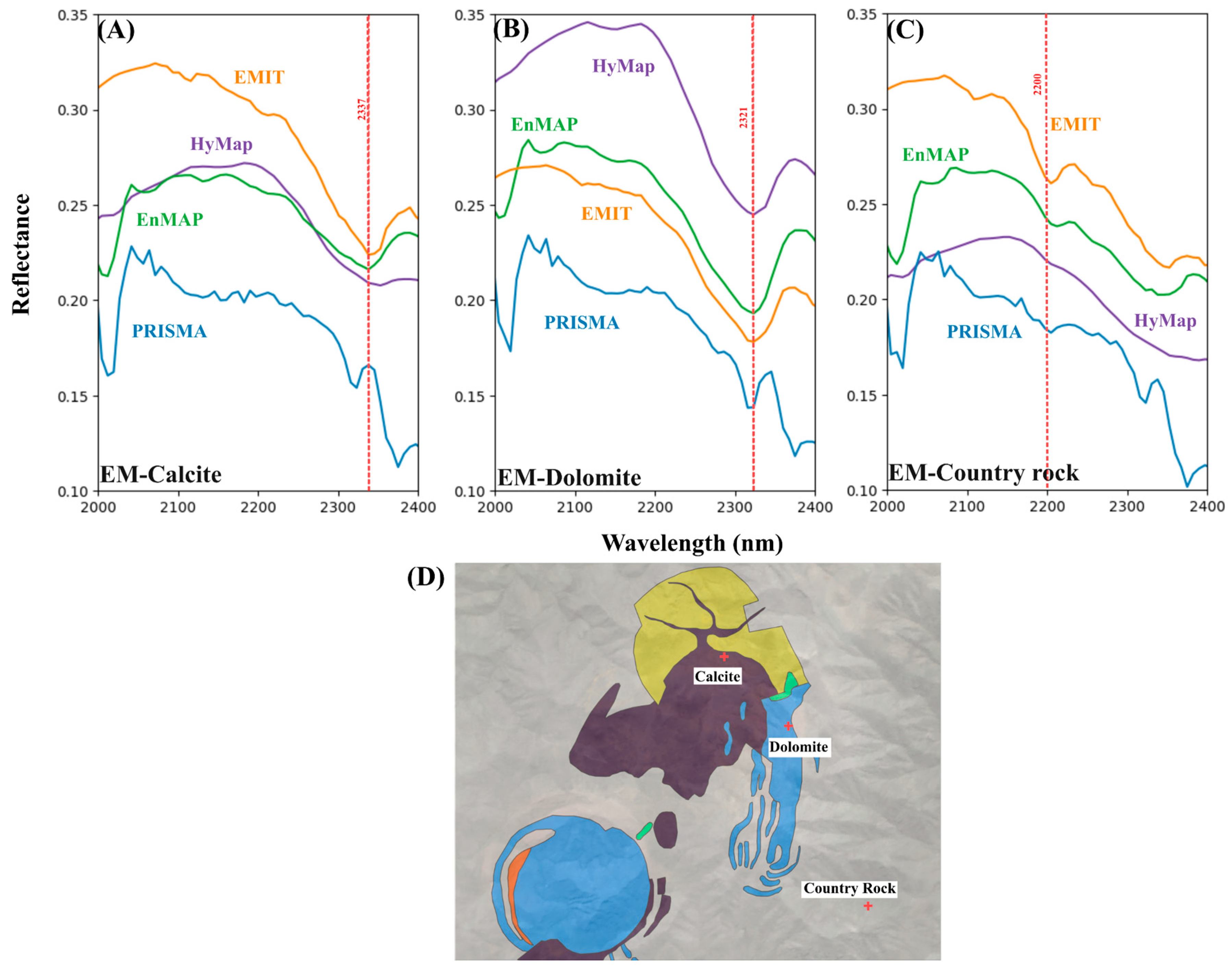
| Calcite | Marinkas-Quellen and Epembe | 2337 nm | [54,55] | |
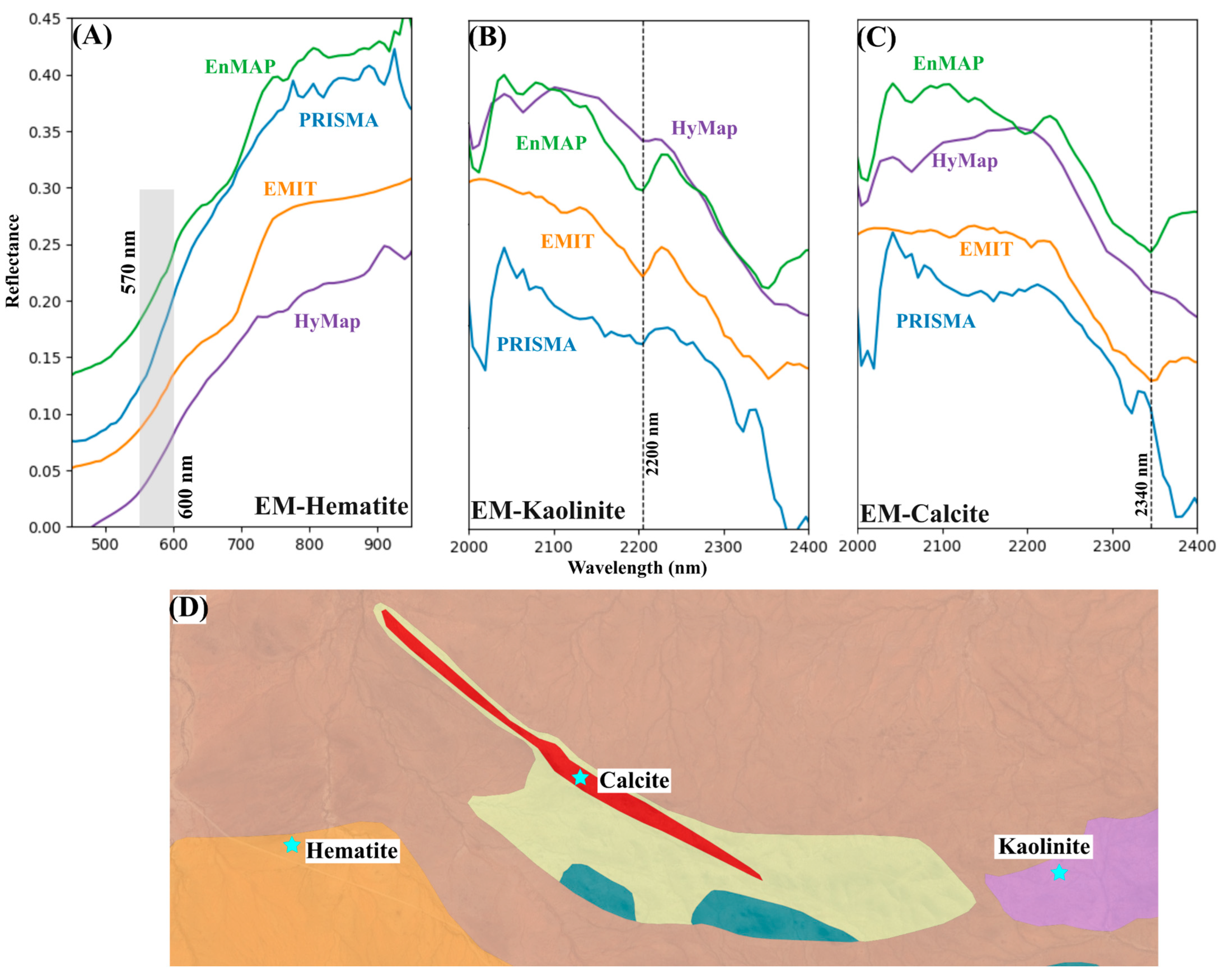
| Hematite | Epembe | 570 nm | [57] | |
| Kaolinite | Epembe | 2195 nm, 2225 nm | [54,55] | |
| Dolomite | Marinkas-Quellen | 2320 nm | [54] |
3.3.2. Spectral Abundance Mapping
3.4. Comparing Sensors by Quantifying Hyperspectral Consistency
4. Results and Interpretation
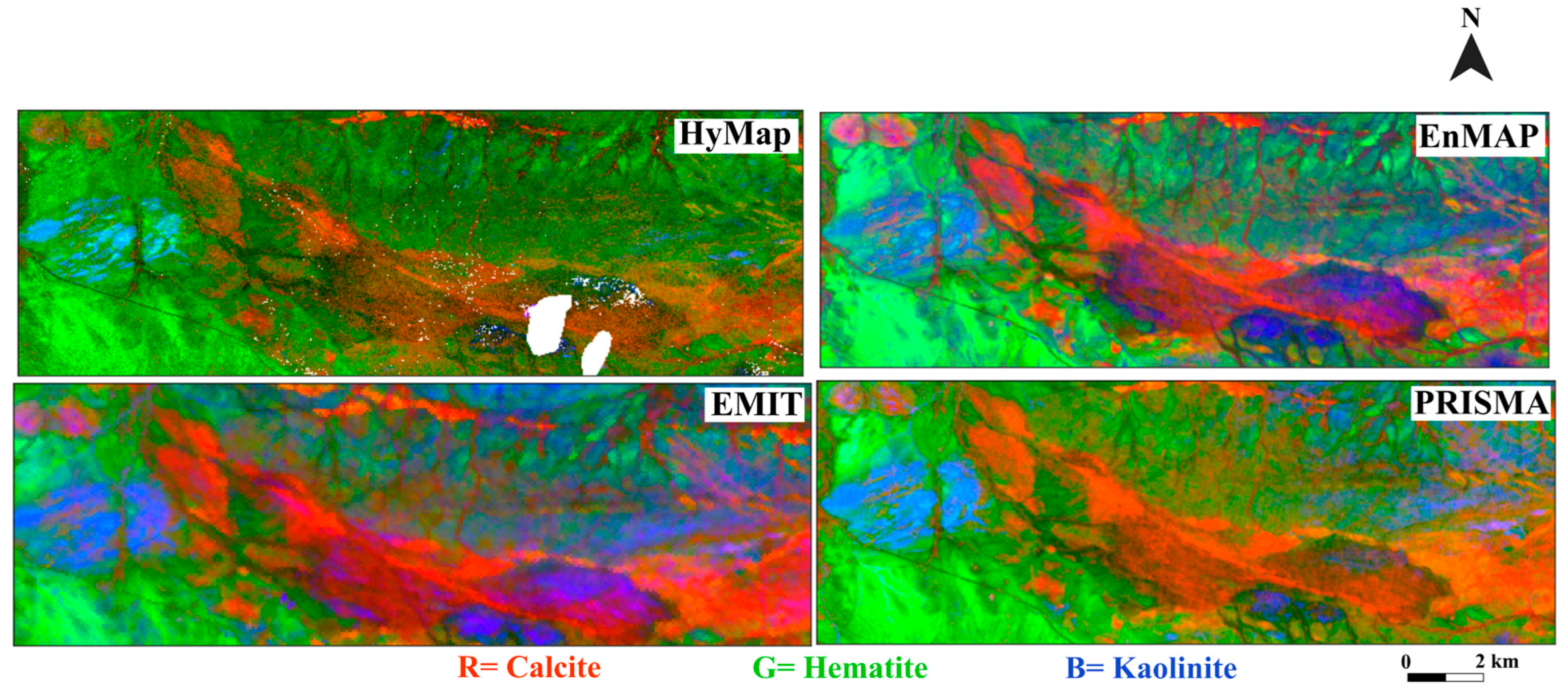
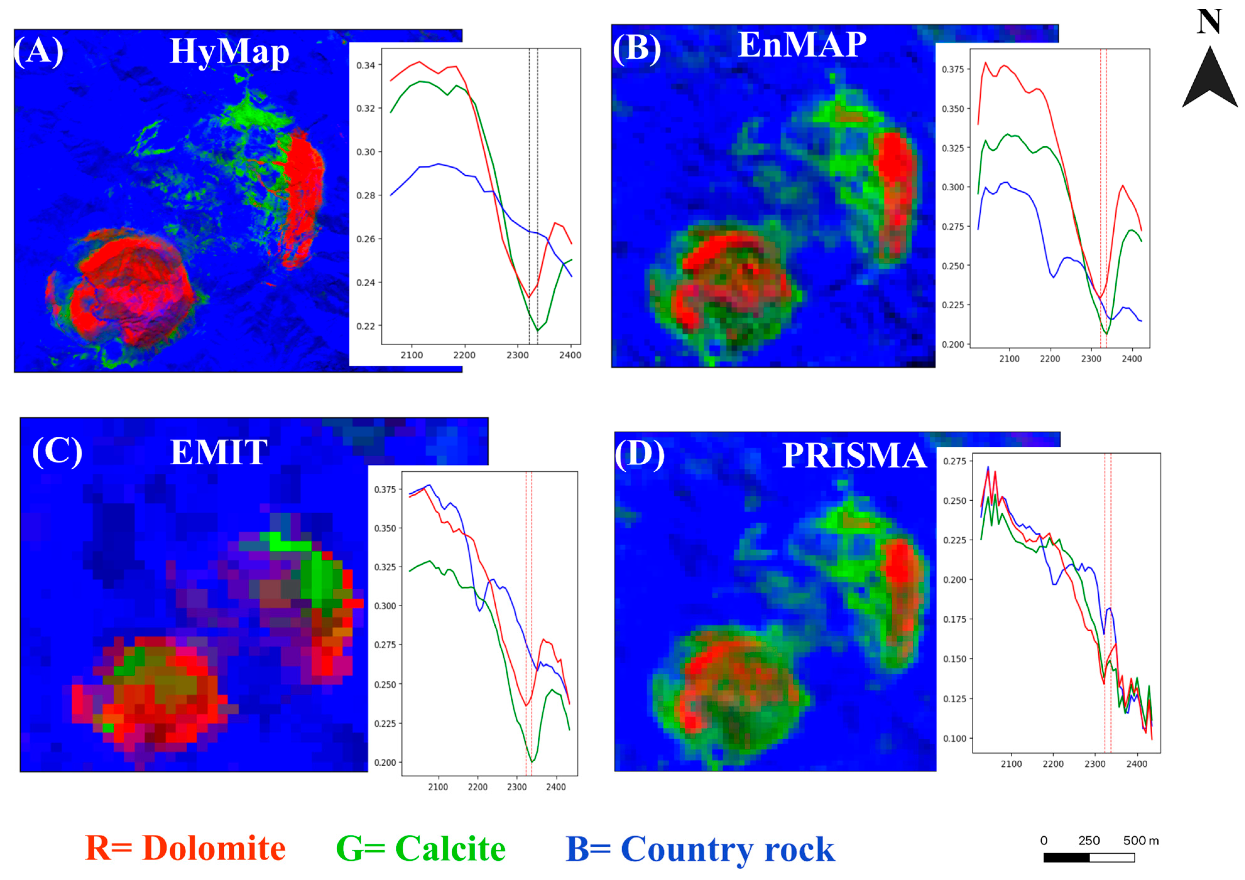
4.1. Qualitative Comparison
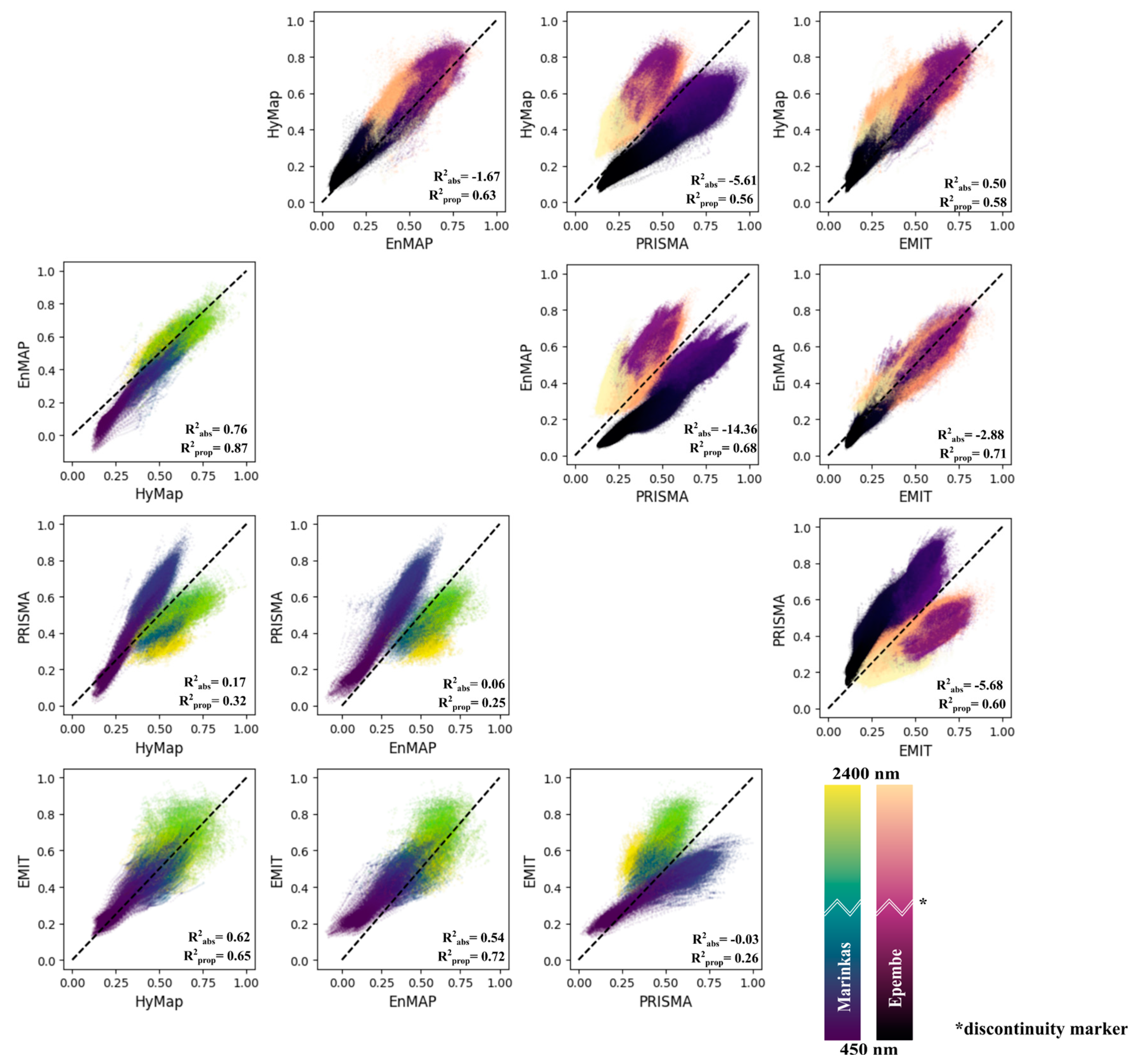
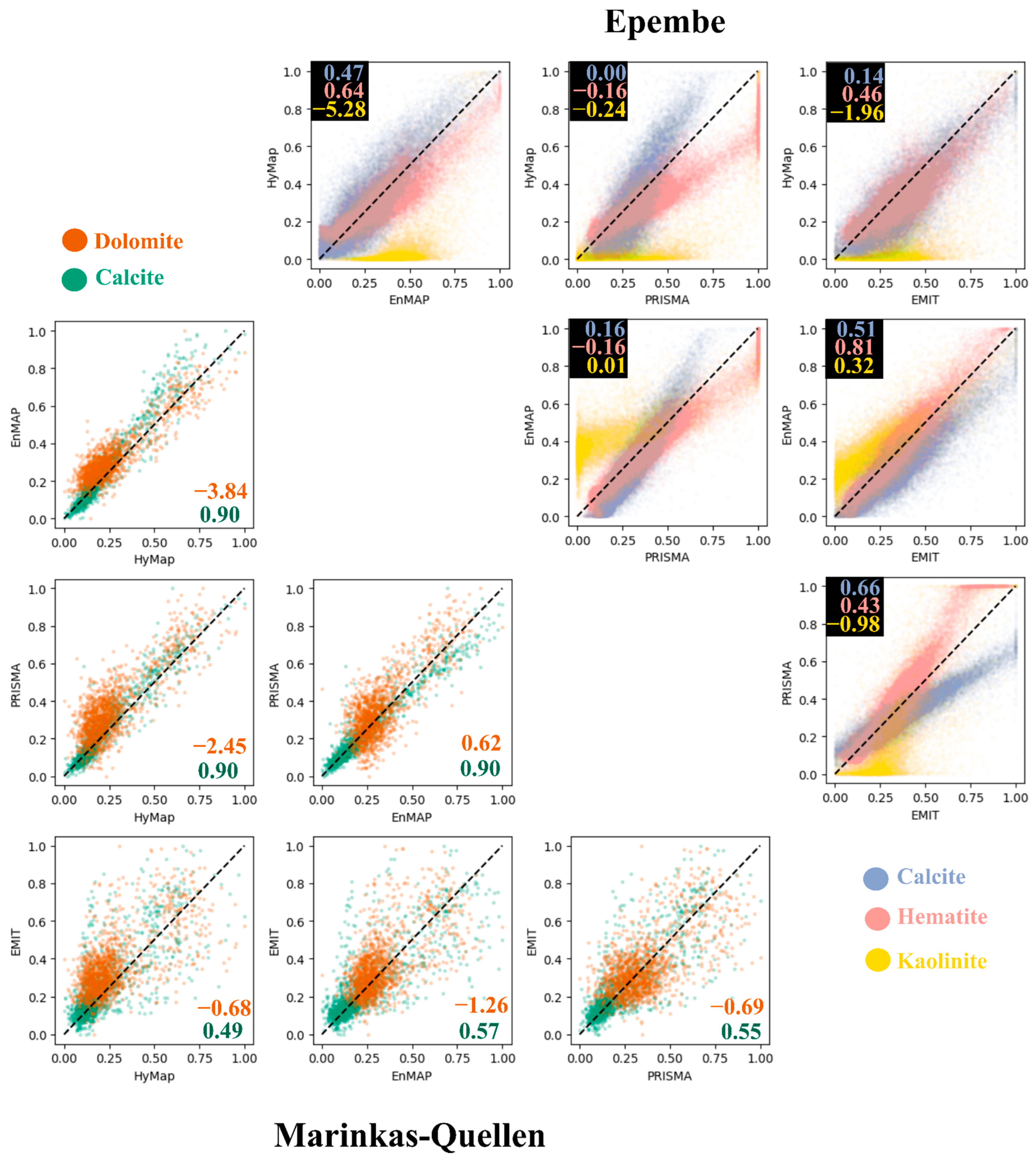
4.2. Absolute and Relative Consistency
4.3. Feature Consistency
4.4. Latent Consistency
5. Discussion
6. Conclusions
Supplementary Materials
Author Contributions
Funding
Data Availability Statement
Acknowledgments
Conflicts of Interest
References
- Cudahy, T.; Jones, M.; Thomas, M.; Laukamp, C.; Caccetta, M.; Hewson, R.; Rodger, A.; Verrall, M. Next Generation Mineral Mapping: Queensland Airborne HyMap and Satellite ASTER Surveys 2006–2008. Commonw. Sci. Ind. Res. Organ. Rep. 2008, 364, 1–161. [Google Scholar]
- Kruse, F.A.; Boardman, J.W.; Huntington, J.F. Comparison of Airborne Hyperspectral Data and EO-1 Hyperion for Mineral Mapping. IEEE Trans. Geosci. Remote Sens. 2003, 41, 1388–1400. [Google Scholar] [CrossRef]
- Kruse, F.A. Advances in Hyperspectral Remote Sensing for Geologic Mapping and Exploration. In Proceedings of the Proceedings 9th Australasian Remote Sensing Conference, Sydney, Australia, 20–24 July 1998. [Google Scholar]
- Lampinen, H.M.; Laukamp, C.; Occhipinti, S.A.; Hardy, L. Mineral Footprints of the Paleoproterozoic Sediment-Hosted Abra Pb-Zn-Cu-Au Deposit Capricorn Orogen, Western Australia. Ore Geol. Rev. 2019, 104, 436–461. [Google Scholar] [CrossRef]
- Laukamp, C.; Rodger, A.; LeGras, M.; Lampinen, H.; Lau, I.C.; Pejcic, B.; Stromberg, J.; Francis, N.; Ramanaidou, E. Mineral Physicochemistry Underlying Feature-Based Extraction of Mineral Abundance and Composition from Shortwave, Mid and Thermal Infrared Reflectance Spectra. Minerals 2021, 11, 347. [Google Scholar] [CrossRef]
- Riihimäki, H.; Luoto, M.; Heiskanen, J. Estimating Fractional Cover of Tundra Vegetation at Multiple Scales Using Unmanned Aerial Systems and Optical Satellite Data. Remote Sens. Environ. 2019, 224, 119–132. [Google Scholar] [CrossRef]
- Clark, R.N. Spectroscopy of Rocks and Minerals, and Principles of Spectroscopy; John Wiley and Sons: Hoboken, NJ, USA, 2020. [Google Scholar]
- van der Meer, F.; Kopačková, V.; Koucká, L.; van der Werff, H.M.; van Ruitenbeek, F.J.; Bakker, W.H. Wavelength Feature Mapping as a Proxy to Mineral Chemistry for Investigating Geologic Systems: An Example from the Rodalquilar Epithermal System. Int. J. Appl. Earth Obs. Geoinf. 2018, 64, 237–248. [Google Scholar] [CrossRef]
- Sabins, F.F. Remote Sensing for Mineral Exploration. Ore Geol. Rev. 1999, 14, 157–183. [Google Scholar] [CrossRef]
- Cloutis, E.A.; Sunshine, J.M.; Morris, R.V. Spectral Reflectance-compositional Properties of Spinels and Chromites: Implications for Planetary Remote Sensing and Geothermometry. Meteorit. Planet. Sci. 2004, 39, 545–565. [Google Scholar] [CrossRef]
- Boesche, N.K.; Rogass, C.; Lubitz, C.; Brell, M.; Herrmann, S.; Mielke, C.; Tonn, S.; Appelt, O.; Altenberger, U.; Kaufmann, H. Hyperspectral REE (Rare Earth Element) Mapping of Outcrops—Applications for Neodymium Detection. Remote Sens. 2015, 7, 5160–5186. [Google Scholar] [CrossRef]
- Chukanov, N.V.; Chervonnyi, A.D. Infrared Spectroscopy of Minerals and Related Compounds; Springer: Berlin/Heidelberg, Germany, 2016; ISBN 3-319-25349-2. [Google Scholar]
- Cudahy, T.; Caccetta, M.; Thomas, M.; Hewson, R.; Abrams, M.; Kato, M.; Kashimura, O.; Ninomiya, Y.; Yamaguchi, Y.; Collings, S. Satellite-Derived Mineral Mapping and Monitoring of Weathering, Deposition and Erosion. Sci. Rep. 2016, 6, 23702. [Google Scholar] [CrossRef]
- Clark, R.N.; King, T.V.; Klejwa, M.; Swayze, G.A.; Vergo, N. High Spectral Resolution Reflectance Spectroscopy of Minerals. J. Geophys. Res. Solid Earth 1990, 95, 12653–12680. [Google Scholar] [CrossRef]
- King, T.V.; Clark, R.N. Spectral Characteristics of Chlorites and Mg-serpentines Using High-resolution Reflectance Spectroscopy. J. Geophys. Res. Solid Earth 1989, 94, 13997–14008. [Google Scholar] [CrossRef]
- Swayze, G.A.; Clark, R.N.; Goetz, A.F.; Livo, K.E.; Breit, G.N.; Kruse, F.A.; Sutley, S.J.; Snee, L.W.; Lowers, H.A.; Post, J.L. Mapping Advanced Argillic Alteration at Cuprite, Nevada, Using Imaging Spectroscopy. Econ. Geol. 2014, 109, 1179–1221. [Google Scholar] [CrossRef]
- Ungar, S.G.; Pearlman, J.S.; Mendenhall, J.A.; Reuter, D. Overview of the Earth Observing One (EO-1) Mission. IEEE Trans. Geosci. Remote Sens. 2003, 41, 1149–1159. [Google Scholar] [CrossRef]
- Liu, L.; Feng, J.; Rivard, B.; Xu, X.; Zhou, J.; Han, L.; Yang, J.; Ren, G. Mapping Alteration Using Imagery from the Tiangong-1 Hyperspectral Spaceborne System: Example for the Jintanzi Gold Province, China. Int. J. Appl. Earth Obs. Geoinf. 2018, 64, 275–286. [Google Scholar] [CrossRef]
- Liu, Y.-N.; Sun, D.-X.; Hu, X.-N.; Ye, X.; Li, Y.-D.; Liu, S.-F.; Cao, K.-Q.; Chai, M.-Y.; Zhang, J.; Zhang, Y. The Advanced Hyperspectral Imager: Aboard China’s gaoFen-5 Satellite. IEEE Geosci. Remote Sens. Mag. 2019, 7, 23–32. [Google Scholar] [CrossRef]
- Iwasaki, A.; Ohgi, N.; Tanii, J.; Kawashima, T.; Inada, H. Hyperspectral Imager Suite (HISUI)-Japanese Hyper-Multi Spectral Radiometer. In Proceedings of the 2011 IEEE International Geoscience and Remote Sensing Symposium, Vancouver, BC, Canada, 24–29 July 2011; pp. 1025–1028. [Google Scholar]
- Thompson, D.R.; Green, R.O.; Bradley, C.; Brodrick, P.G.; Dor, B.; Bennett, M.; Bernas, M.; Carmon, N.; Chadwick, K.D.; Clark, R.N. On-Orbit Calibration and Performance of the EMIT Imaging Spectrometer. ESS Open Arch. 2023, 10, 1–16. [Google Scholar] [CrossRef]
- Kerr, G.; Avbelj, J.; Carmona, E.; Eckardt, A.; Gerasch, B.; Graham, L.; Günther, B.; Heiden, U.; Krutz, D.; Krawczyk, H. The Hyperspectral Sensor DESIS on MUSES: Processing and Applications. In Proceedings of the 2016 IEEE International Geoscience and Remote Sensing Symposium (IGARSS), Beijing, China, 10–15 July 2016; pp. 268–271. [Google Scholar]
- Lee, K.-H.; Yum, J.-M. A Review on Atmospheric Correction Technique Using Satellite Remote Sensing. Korean J. Remote Sens. 2019, 35, 1011–1030. [Google Scholar]
- Thiele, S.T.; Bnoulkacem, Z.; Lorenz, S.; Bordenave, A.; Menegoni, N.; Madriz, Y.; Dujoncquoy, E.; Gloaguen, R.; Kenter, J. Mineralogical Mapping with Accurately Corrected Shortwave Infrared Hyperspectral Data Acquired Obliquely from UAVs. Remote Sens. 2021, 14, 5. [Google Scholar] [CrossRef]
- Bohn, N.; Brodrick, P.; Montgomery, J.; Thompson, D. Advances in Imaging Spectrometer Atmospheric Correction with the Open-Source ISOFIT Codebase. In Proceedings of the IGARSS 2023-2023 IEEE International Geoscience and Remote Sensing Symposium, Pasadena, CA, USA, 16–21 July 2023; pp. 1253–1256. [Google Scholar]
- Smithies, R.H. The Geochemical Evolution of Three Alkaline Complexes in the Kuboos-Bremen Igneous Province, Southern Namibia; Rhodes University: Makhanda, South Africa, 1991. [Google Scholar]
- Verwoerd, W.J. Update on Carbonatites of South Africa and Namibia. S. Afr. J. Geol. 1993, 96, 75–95. [Google Scholar]
- Miller, R.M. The Geology of Namibia; Ministry of Mines and Energy, Geological Survey: Windhoek, Namibia, 2008; Volume 1.
- Zimmermann, R.; Brandmeier, M.; Andreani, L.; Mhopjeni, K.; Gloaguen, R. Remote Sensing Exploration of Nb-Ta-LREE-Enriched Carbonatite (Epembe/Namibia). Remote Sens. 2016, 8, 620. [Google Scholar] [CrossRef]
- Smithies, R.H.; Marsh, J.S. The Marinkas Quellen Carbonatite Complex, Southern Namibia; Carbonatite Magmatism with an Uncontaminated Depleted Mantle Signature in a Continental Setting. Chem. Geol. 1998, 148, 201–212. [Google Scholar] [CrossRef]
- González-Álvarez, I.; Stoppa, F.; Yang, X.Y.; Porwal, A. Introduction to the Special Issue, Insights on Carbonatites and Their Mineral Exploration Approach: A Challenge towards Resourcing Critical Metals. Ore Geol. Rev. 2021, 133, 104073. [Google Scholar] [CrossRef]
- Jones, A.P.; Genge, M.; Carmody, L. Carbonate Melts and Carbonatites. Rev. Mineral. Geochem. 2013, 75, 289–322. [Google Scholar] [CrossRef]
- Winter, J.D. Principles of Igneous and Metamorphic Petrology; Pearson Education: Harlow, UK, 2014; Volume 2. [Google Scholar]
- Booysen, R.; Jackisch, R.; Lorenz, S.; Zimmermann, R.; Kirsch, M.; Nex, P.A.M.; Gloaguen, R. Detection of REEs with Lightweight UAV-Based Hyperspectral Imaging. Sci. Rep. 2020, 10, 17450. [Google Scholar] [CrossRef] [PubMed]
- Lorenz, S.; Beyer, J.; Fuchs, M.; Seidel, P.; Turner, D.; Heitmann, J.; Gloaguen, R. The Potential of Reflectance and Laser Induced Luminescence Spectroscopy for Near-Field Rare Earth Element Detection in Mineral Exploration. Remote Sens. 2018, 11, 21. [Google Scholar] [CrossRef]
- Rowan, L.C.; Kingston, M.J.; Crowley, J.K. Spectral Reflectance of Carbonatites and Related Alkalic Igneous Rocks; Selected Samples from Four North American Localities. Econ. Geol. 1986, 81, 857–871. [Google Scholar] [CrossRef]
- White, W.B. Diffuse-Reflectance Spectra of Rare-Earth Oxides. Appl. Spectrosc. 1967, 21, 167–171. [Google Scholar] [CrossRef]
- Littmann, S.; Cook, N.; Teigler, B.; Drüppel, K. Ultramafic/Mafic Intrusives Hosting Cu-Ni Sulphide Mineralisation, Itjitambi Area, Kunene Region, NW Namibia: Investigation of Drillcore, Hole OTD-1. Commun. Geol. Surv. Namib. 2003. [Google Scholar]
- Brandt, S.; Will, T.M.; Klemd, R. Magmatic Loading in the Proterozoic Epupa Complex, NW Namibia, as Evidenced by Ultrahigh-Temperature Sapphirine-Bearing Orthopyroxene–Sillimanite–Quartz Granulites. Precambrian Res. 2007, 153, 143–178. [Google Scholar] [CrossRef]
- Unger, G.; Zimmermann, R.; Gloaguen, R. 3D Modeling of the Epembe (Namibia) Nb-Ta-P-(LREE) Carbonatite Deposit: New Insights into Geometry Related to Rare Metal Enrichment. Minerals 2018, 8, 600. [Google Scholar] [CrossRef]
- Guarini, R.; Loizzo, R.; Longo, F.; Mari, S.; Scopa, T.; Varacalli, G. Overview of the Prisma Space and Ground Segment and Its Hyperspectral Products. In Proceedings of the 2017 IEEE International Geoscience and Remote Sensing Symposium (IGARSS), Fort Worth, TX, USA, 23–28 July 2017; pp. 431–434. [Google Scholar]
- De Los Reyes, R.; Langheinrich, M.; Schwind, P.; Richter, R.; Pflug, B.; Bachmann, M.; Müller, R.; Carmona, E.; Zekoll, V.; Reinartz, P. PACO: Python-Based Atmospheric Correction. Sensors 2020, 20, 1428. [Google Scholar] [CrossRef] [PubMed]
- de Los Reyes, R.; Langheinrich, M.; Alonso, K.; Bachmann, M.; Carmona, E.; Gerasch, B.; Holzwarth, S.; Marshall, D.; Müller, R.; Pato, M. Atmospheric Correction of DESIS and EnMAP Hyperspectral Data: Validation of L2a Products. In Proceedings of the IGARSS 2023-2023 IEEE International Geoscience and Remote Sensing Symposium, Pasadena, CA, USA, 16–21 July 2023; pp. 1034–1037. [Google Scholar]
- Richter, R.; Schlapfer, D. Atmospheric/Topographic Correction for Satellite Imagery; ATCOR-2/3 User Guide; Remote Sensing Applications: Wil, Switzerland, 2023. [Google Scholar]
- Cawse-Nicholson, K.; Townsend, P.A.; Schimel, D.; Assiri, A.M.; Blake, P.L.; Buongiorno, M.F.; Campbell, P.; Carmon, N.; Casey, K.A.; Correa-Pabón, R.E.; et al. NASA’s Surface Biology and Geology Designated Observable: A Perspective on Surface Imaging Algorithms. Remote Sens. Environ. 2021, 257, 112349. [Google Scholar] [CrossRef]
- Scheffler, D.; Hollstein, A.; Diedrich, H.; Segl, K.; Hostert, P. AROSICS: An Automated and Robust Open-Source Image Co-Registration Software for Multi-Sensor Satellite Data. Remote Sens. 2017, 9, 676. [Google Scholar] [CrossRef]
- Gillies, S. Rasterio Documentation. MapBox. 23 July 2019. Available online: https://readthedocs.org/projects/rasterio/downloads/pdf/latest/ (accessed on 13 May 2024).
- Pedregosa, F.; Varoquaux, G.; Gramfort, A.; Michel, V.; Thirion, B.; Grisel, O.; Blondel, M.; Prettenhofer, P.; Weiss, R.; Dubourg, V. Scikit-Learn: Machine Learning in Python. J. Mach. Learn. Res. 2011, 12, 2825–2830. [Google Scholar]
- Geranian, H.; Tabatabaei, S.H.; Asadi, H.H.; Carranza, E.J.M. Application of Discriminant Analysis and Support Vector Machine in Mapping Gold Potential Areas for Further Drilling in the Sari-Gunay Gold Deposit, NW Iran. Nat. Resour. Res. 2016, 25, 145–159. [Google Scholar] [CrossRef]
- Kereszturi, G.; Schaefer, L.N.; Miller, C.; Mead, S. Hydrothermal Alteration on Composite Volcanoes: Mineralogy, Hyperspectral Imaging, and Aeromagnetic Study of Mt Ruapehu, New Zealand. Geochem. Geophys. Geosyst. 2020, 21, e2020GC009270. [Google Scholar] [CrossRef]
- Thiele, S.T.; Lorenz, S.; Kirsch, M.; Cecilia Contreras Acosta, I.; Tusa, L.; Herrmann, E.; Möckel, R.; Gloaguen, R. Multi-Scale, Multi-Sensor Data Integration for Automated 3-D Geological Mapping. Ore Geol. Rev. 2021, 136, 104252. [Google Scholar] [CrossRef]
- Sadiya, T.B.; Ibrahim, O.; Asma, T.F.; Mamfe, V.; Nsofor, C.J.; Oyewmi, A.S.; Shar, J.T.; Sanusi, M.; Ozigis, M.S. Mineral Detection and Mapping Using Band Ratioing and Crosta Technique in Bwari Area Council, Abuja Nigeria. Int. J. Sci. Eng. Res. 2014, 5, 1100–1108. [Google Scholar]
- Goetz, A.F.; Billingsley, F.C.; Gillespie, A.R.; Abrams, M.J.; Squires, R.L.; Shoemaker, E.M.; Lucchitta, I.; Elston, D.P. Application of ERTS Images and Image Processing to Regional Geologic Problems and Geologic Mapping in Northern Arizona; Jet Propulsion Laboratory: Pasadena, CA, USA, 1975. [Google Scholar]
- Laukamp, C. Geological Mapping Using Mineral Absorption Feature-Guided Band-Ratios Applied to Prisma Satellite Hyperspectral Level 2D Imagery. In Proceedings of the IGARSS 2022–2022 IEEE International Geoscience and Remote Sensing Symposium, Kuala Lumpur, Malaysia, 17–22 July 2022; pp. 5981–5984. [Google Scholar]
- Zhang, X.; Pazner, M.; Duke, N. Lithologic and Mineral Information Extraction for Gold Exploration Using ASTER Data in the South Chocolate Mountains (California). ISPRS J. Photogramm. Remote Sens. 2007, 62, 271–282. [Google Scholar] [CrossRef]
- Sorrentino, A.; Chirico, R.; Corrado, F.; Laukamp, C.; Di Martire, D.; Mondillo, N. The Application of PRISMA Hyperspectral Satellite Imagery in the Delineation of Distinct Hydrothermal Alteration Zones in the Chilean Andes: The Marimaca IOCG and the Río Blanco-Los Bronces Cu-Mo Porphyry Districts. Ore Geol. Rev. 2024, 167, 105998. [Google Scholar] [CrossRef]
- Chirico, R.; Mondillo, N.; Laukamp, C.; Mormone, A.; Di Martire, D.; Novellino, A.; Balassone, G. Mapping Hydrothermal and Supergene Alteration Zones Associated with Carbonate-Hosted Zn-Pb Deposits by Using PRISMA Satellite Imagery Supported by Field-Based Hyperspectral Data, Mineralogical and Geochemical Analysis. Ore Geol. Rev. 2023, 152, 105244. [Google Scholar] [CrossRef]
- Ghamisi, P.; Yokoya, N.; Li, J.; Liao, W.; Liu, S.; Plaza, J.; Rasti, B.; Plaza, A. Advances in Hyperspectral Image and Signal Processing: A Comprehensive Overview of the State of the Art. IEEE Geosci. Remote Sens. Mag. 2017, 5, 37–78. [Google Scholar] [CrossRef]
- Keshava, N.; Mustard, J.F. Spectral Unmixing. IEEE Signal Process. Mag. 2002, 19, 44–57. [Google Scholar] [CrossRef]
- Song, K.; Wang, E.; Yao, Y.; Fu, J.; Hao, D.; You, X. Spectral Alteration Zonation Based on Close Range Hyspex-320 m Imaging Spectroscopy: A Case Study in the Gongchangling High-Grade Iron Ore Deposit, Liaoning Province, NE China. Appl. Sci. 2020, 10, 8369. [Google Scholar] [CrossRef]
- Tuşa, L.; Khodadadzadeh, M.; Contreras, C.; Rafiezadeh Shahi, K.; Fuchs, M.; Gloaguen, R.; Gutzmer, J. Drill-Core Mineral Abundance Estimation Using Hyperspectral and High-Resolution Mineralogical Data. Remote Sens. 2020, 12, 1218. [Google Scholar] [CrossRef]
- Therien, C. Welcome to the PySptools Documentation; Christian Therien: Montreal, QC, Canada, 2021. [Google Scholar]
- Chang, C.-I.; Wu, C.-C.; Tsai, C.-T. Random N-Finder (N-FINDR) Endmember Extraction Algorithms for Hyperspectral Imagery. IEEE Trans. Image Process. 2010, 20, 641–656. [Google Scholar] [CrossRef]
- Tapete, D.; Jaiswal, R.K.; Licciardi, G.; Sacco, P.; Gupta, P.K.; Raju, P.V.; Raj, B.G.; Sahadevan, A.S.; Ahmad, T.; Lyngdoh, R.B. Scientific Research and Applications Development Based on Exploitation of PRISMA Data in the Framework of ASI–ISRO Earth Observation Working Group Hyperspectral Activity. In Proceedings of the IGARSS 2023-2023 IEEE International Geoscience and Remote Sensing Symposium, Pasadena, CA, USA, 16–21 July 2023; pp. 1648–1651. [Google Scholar]
- Vangi, E.; D’Amico, G.; Francini, S.; Giannetti, F.; Lasserre, B.; Marchetti, M.; Chirici, G. The New Hyperspectral Satellite PRISMA: Imagery for Forest Types Discrimination. Sensors 2021, 21, 1182. [Google Scholar] [CrossRef]


| EnMAP | EMIT | PRISMA | HyMap | ||
|---|---|---|---|---|---|
| Spatial resolution (in m) | 30 | 60 | 30 | 5 | |
| Spectral sampling (in nm) | VNIR | 6.5 | 7.4 | 12 | 15 |
| SWIR | 10 | 7.4 | 12 | 13–17 | |
| Spectral range (in nm) | VNIR | 420–1000 | 381–2493 | 400–1010 | 450–1350 |
| SWIR | 900–2450 | 920–2505 | 1400–2480 | ||
| Spectral bands | VNIR | 101 | 285 | 66 | 125 |
| SWIR | 123 | 171 | |||
| EnMAP | EMIT | PRISMA | HyMap | ||
|---|---|---|---|---|---|
| Processing level | L2A | L2A RFL | L2D | Reflectance data | |
| Acquisition date | Marinkas Quellen | 17 May 2023 | 7 January 2023 | 21 October 2020 | 26 February 2018 |
| Epembe | 17 April 2023 | 3 May 2023 | 27 November 2022 | 6 August 2014 | |
| Acquisition time (local) | Marinkas Quellen | 11:29 | 10:24 | 11:05 | 14:20 |
| Epembe | 11:49 | 12:01 | 11:27 | 11:52 | |
Disclaimer/Publisher’s Note: The statements, opinions and data contained in all publications are solely those of the individual author(s) and contributor(s) and not of MDPI and/or the editor(s). MDPI and/or the editor(s) disclaim responsibility for any injury to people or property resulting from any ideas, methods, instructions or products referred to in the content. |
© 2024 by the authors. Licensee MDPI, Basel, Switzerland. This article is an open access article distributed under the terms and conditions of the Creative Commons Attribution (CC BY) license (https://creativecommons.org/licenses/by/4.0/).
Share and Cite
Chakraborty, R.; Rachdi, I.; Thiele, S.; Booysen, R.; Kirsch, M.; Lorenz, S.; Gloaguen, R.; Sebari, I. A Spectral and Spatial Comparison of Satellite-Based Hyperspectral Data for Geological Mapping. Remote Sens. 2024, 16, 2089. https://doi.org/10.3390/rs16122089
Chakraborty R, Rachdi I, Thiele S, Booysen R, Kirsch M, Lorenz S, Gloaguen R, Sebari I. A Spectral and Spatial Comparison of Satellite-Based Hyperspectral Data for Geological Mapping. Remote Sensing. 2024; 16(12):2089. https://doi.org/10.3390/rs16122089
Chicago/Turabian StyleChakraborty, Rupsa, Imane Rachdi, Samuel Thiele, René Booysen, Moritz Kirsch, Sandra Lorenz, Richard Gloaguen, and Imane Sebari. 2024. "A Spectral and Spatial Comparison of Satellite-Based Hyperspectral Data for Geological Mapping" Remote Sensing 16, no. 12: 2089. https://doi.org/10.3390/rs16122089
APA StyleChakraborty, R., Rachdi, I., Thiele, S., Booysen, R., Kirsch, M., Lorenz, S., Gloaguen, R., & Sebari, I. (2024). A Spectral and Spatial Comparison of Satellite-Based Hyperspectral Data for Geological Mapping. Remote Sensing, 16(12), 2089. https://doi.org/10.3390/rs16122089