Abstract
As a consequence of global climate change, sea level rise (SLR) presents notable risks to both urban and natural areas located near coastlines. For developing effective strategies to mitigate and adapt to these risks, it is essential to evaluate the potential impacts of SLR in coastal areas. While substantial research has been conducted on mapping the broad-scale impacts of SLR based on scenarios of Global Mean Sea Level (GMSL), consideration of regional scenarios, systematic classification, and distinct stages of SLR have been largely overlooked. This gap is significant because SLR impacts vary by region and by the level of SLR, so adaptations, planning, and decision-making must be adapted to local conditions. This paper aims to precisely identify the landscape and urban morphology changes caused by the impact of SLR for each foot of elevation increase based on remote sensing technologies, focusing on St. Johns County, Florida, and Chatham County, Georgia. These two counties are both situated along the southeastern coastline of the United States but with completely different urban forms due to distinct historical and cultural developments. Regional forecasting SLR scenarios covering the period from 2020 to 2100 were utilized to assess the landscape transformation and urban changes, incorporating selected landscape and urban metrics to calculate quantitative data for facilitating comparative analyses. This study investigated gradual alterations in urban morphology and green infrastructure both individually and in combination with the effect on wetlands due to SLR. The mapping outcomes of this research were generated by employing comprehensive remote sensing data. The findings of this research indicated that, when the sea level rose to 3 feet, the wetlands would experience notable alterations, and the level of fragmentation in urban built areas would progressively increase, causing most of the metric data to exhibit a pronounced decline or increase.
1. Introduction
Sea level rise (SLR) poses a significant risk to urban and natural areas near coastlines. By the year 2100, it is estimated that SLR could reach 0.9 m (2.95 feet), potentially leading to the submergence of coastal areas and impacting around 4.2 million people in the United States [1]. Simultaneously, the form of coastal cities and the pattern of green infrastructure will undergo significant transformation due to the impact of SLR. For example, a one-meter SLR would result in the inundation of 42% of the Albemarle Pamlico Peninsula in North Carolina [2]. Areas that were once habitable may become uninhabitable due to frequent flooding, leading to changes in land-use patterns and urban boundaries. It is essential to study the change in urban morphology and green infrastructure, as they provide valuable insights into the dynamic nature of cities and landscapes, as well as their evolving spatial and structural characteristics. Currently, there exist specific tools that employ computational and information techniques to visualize coastal transformations, such as Sea Level Rise Viewer (NOAA) [3], Surging Seas (Climate Central) [4], and others. However, most of the visualization tools are based on the Global Mean Sea Level (GMSL) rise scenarios, which only take ice sheet loss as the dominant contributor to SLR [5]. The objective of this research is to precisely identify and quantify the landscape and urban form changes caused by the impact of SLR for each foot of elevation increase based on more comprehensive scenarios that consider shifts in oceanographic factors, changes in the Earth’s gravitational field, and vertical land movement [6]. According to the projections of this scenario from the year 2022 in Florida and Georgia, SLR will vary from 0.39 feet in the year 2020 to 6.99 feet in the year 2100 (the most extreme case). The table below (Table 1) shows the regional SLR scenarios from 2020 to 2100 at Fort Pulaski, Chatham County, GA.

Table 1.
Regional sea level rise scenarios at Fort Pulaski, GA, viewed by year in feet (2022 projections).
Specific numerical experiments have demonstrated that, once a certain threshold of SLR is exceeded, inundation results in an irreversible transformation of intertidal marshland into unvegetated areas. In five numerical models [7,8,9,10,11] aimed at investigating the long-term evolution of coastal marshland, considering feedback between inundation, sediment deposition, and the interplay of physical and biological processes, the consensus is that, by around the year 2080, accretion rates will decline to a level where they can no longer sustain vegetation [12]. The local intermediate SLR around the year 2080 would be 2.56 feet (Table 1).
Landscape metrics provide a quantitative way to assess changes in the natural and human environment detected by remote sensing technology. These metrics enable researchers to precisely measure the extent and magnitude of these changes, which are essential for understanding the impacts of SLR. They offer a systematic and data-driven approach to understanding changes in both natural and built environments for studying and addressing the impacts of SLR. FRAGSTATS [13] is a software program created for the purpose of calculating a diverse range of landscape metrics, aimed at enhancing our comprehension of landscape fragmentation. Metrics in this software can quantify attributes such as area, shape, core area, nearest-neighbor distances, isolation, and connectedness at the patch, class, or landscape level [14,15,16,17]. The software has been widely used in quantifying the configuration, fragmentation, and connectivity of landscape patterns [18,19]. In addition, FRAGSTATS metrics have been used in land-use change studies correlated to the degree of urbanization, development, and water quality [20]. However, some researchers indicated that the majority of papers utilizing landscape metrics or indices focus on biodiversity and habitat analysis [21], while fewer studies are related to the built environment and impacts of SLR.
The study of urban morphology and green infrastructure focuses on two different aspects of urban and natural landscape planning. Urban morphology studies the formation and transformation of urban forms in cities, towns, and villages over time [22]. Alternatively, green infrastructure focuses on open spaces, watersheds, wildlife habitats, parks, and other critical landscapes. Both types of studies are affected by several factors such as urban history, culture, and geography, as well as natural resources. In the study of urban and natural landscapes in relation to SLR, much of the literature tends to focus on either cities or natural landscapes, but not both. For instance, some studies concentrate on urban planning adaptations to SLR [23], while others address coastal wetland adaptation [24]. However, for holistic urban development, it is essential to integrate both disciplines. They are most effective when considered together, and the decision-making process should account for the relationship and degree of change between them. The study areas are St. Johns County in Florida and Chatham County in Georgia. The two counties are both located on extensive low-lying coastal areas of the southeastern United States, dominated by saltwater marshes, estuaries, and barrier islands. These low elevations make them highly vulnerable to rising sea levels, leading to a greater risk of flooding and coastal erosion. Florida has the second longest coastline among all the states in the United States [25], with a high proportion already developed, while Georgia, with a lower amount of coastline, has been more effective than Florida in preserving some of its valuable coastal ecosystems. Moreover, having a rich history that goes back to the foundation of the United States, the two counties contain valuable cultural, archaeological, and historical heritage, including architectural landmarks, artifacts, and cultural sites. Rising sea levels can pose a threat to these structures, leading to potential loss or damage. Especially with distinct establishment purposes, the two counties employed entirely different planning approaches, leading to noticeable disparities in their vulnerability to SLR. Within a framework for investigating urban morphologies and landscape change [26], an understanding focused on relations between places rather than only within the places themselves was applied in this paper.
The objective of this study is to employ remote sensing technologies for mapping and quantifying changes in urban morphology and landscapes in response to the gradual rise of sea levels along the southeastern coast of the United States, specifically focusing on St. Johns County in Florida and Chatham County in Georgia.
To address the identified research gaps, this study’s principal strengths include the following:
- This research addressed a critical gap in SLR studies for coastal landscape assessment, planning, and decision-making by incorporating remote sensing-based land-use/land-cover changes, mapped with regional and comprehensive SLR scenarios projected up to the year 2100 [6];
- In addition to maps, our analysis also quantified natural landscape and urban changes based on numerical landscape metrics, enabling objective comparisons and statistical summaries beyond visual map interpretations.
- The geospatial methodology and findings utilizing remote sensing data in this study served not only as a reference for comprehensive planning but also as a basis for crafting distinct adaptation strategies for urban and natural landscapes.
2. Literature Review
2.1. Sea Level Rise (SLR) Scenarios
In general, SLR scenarios are based on climate model outputs. Parris and other authors [5] described four global mean SLR scenarios (Highest, Intermediate–High, Intermediate–Low, and Lowest) for assessing potential vulnerabilities and impacts. The Intergovernmental Panel on Climate Change also released global mean sea level rise scenarios with its 6th Assessment Report (AR6) [27]. The NASA Sea Level Projection Tool, which visualizes sea level projections, was developed based on the Intergovernmental Panel on Climate Change’s 6th Assessment Report [28]. These scenarios provide coastal managers with the most authoritative information about SLR in the future [29]. The sea level rise and Coastal Flood Hazard Scenarios we applied to this study are based on the Parris et al. [5] and Sweet et al. [6] 2012 and 2022 global mean SLR (GMSL) scenarios. The authors updated the scenarios and integrated the scenarios with regional factors that contribute to sea level change for the entire U.S. coastline. To distinguish bewteen different types of planning scenarios, the most important aspect is to ensure that the scenarios are designed from different perspectives. The Intergovernmental Panel on Climate Change scenarios assumed that thermal expansion is the dominant contributor, while Parris’ GMSL scenarios are based on the National Research Council reports, which indicated that, from 1993 to 2008, ice sheet loss was a greater contribution to global SLR than thermal expansion. While the scenarios we applied were based on the GMSL rise scenarios and regional factors in the USA, they addressed a major gap in climate information needed for assessment, planning, and decision-making. For our study areas that are located near the southeast coast, under the Intermediate–High, High, and Extreme scenarios, relative SLR is projected to exceed the global average. Moreover, for this scenario/model, NOAA provides detailed data that can be used for research analysis [3].
2.2. Natural Landscape and Urban Metrics
In the nearly 30 years since FRAGSTATS [13] was released, this software for calculating landscape metrics has helped to revolutionize the analysis of landscape structure. Nowadays, many land managers and stakeholders still regard it as a simple and intuitive tool for assessing and monitoring changes in landscape patterns [30]. FRAGSTATS has been widely applied in studies regarding climate change and urbanization. For example, it was applied to explore long-term morphological changes in climatic landscapes on a global and continental scale [31]. Metrics like fragmentation, area-edge, shape, and aggregation were applied to measure the effects of green area landscape patterns on public health [32]. And, for urbanization studies, the spatial landscape metrics approach and Shannon’s entropy model have been applied for analyzing the urban growth pattern [33]. Ten landscape metrics, such as percentage of landscape and patch density, have been selected to explore the spatiotemporal patterns of land-use change in Swiss urban agglomerations [34]. With the increasing focus on SLR, landscape metrics are being used more frequently in this field. In 2011, a method that included landscape metrics was developed and applied to assess and compare various land-use scenarios for flood prevention and nature conservation [35]. Landscape metrics were also used to predict surface hydrologic connectivity patterns [36]. However, considering integrated impact assessment, research that focuses on both urban built areas and natural landscapes simultaneously would be able to provide holistic adaptation strategies related to SLR. This study aims to apply landscape metrics computed in FRAGSTATS to both urban and natural landscape change analysis. The research outputs combined efforts in both areas to consider overall resilience and contribute more effectively to climate change mitigation and adaptation.
3. Materials and Methods
3.1. Study Areas
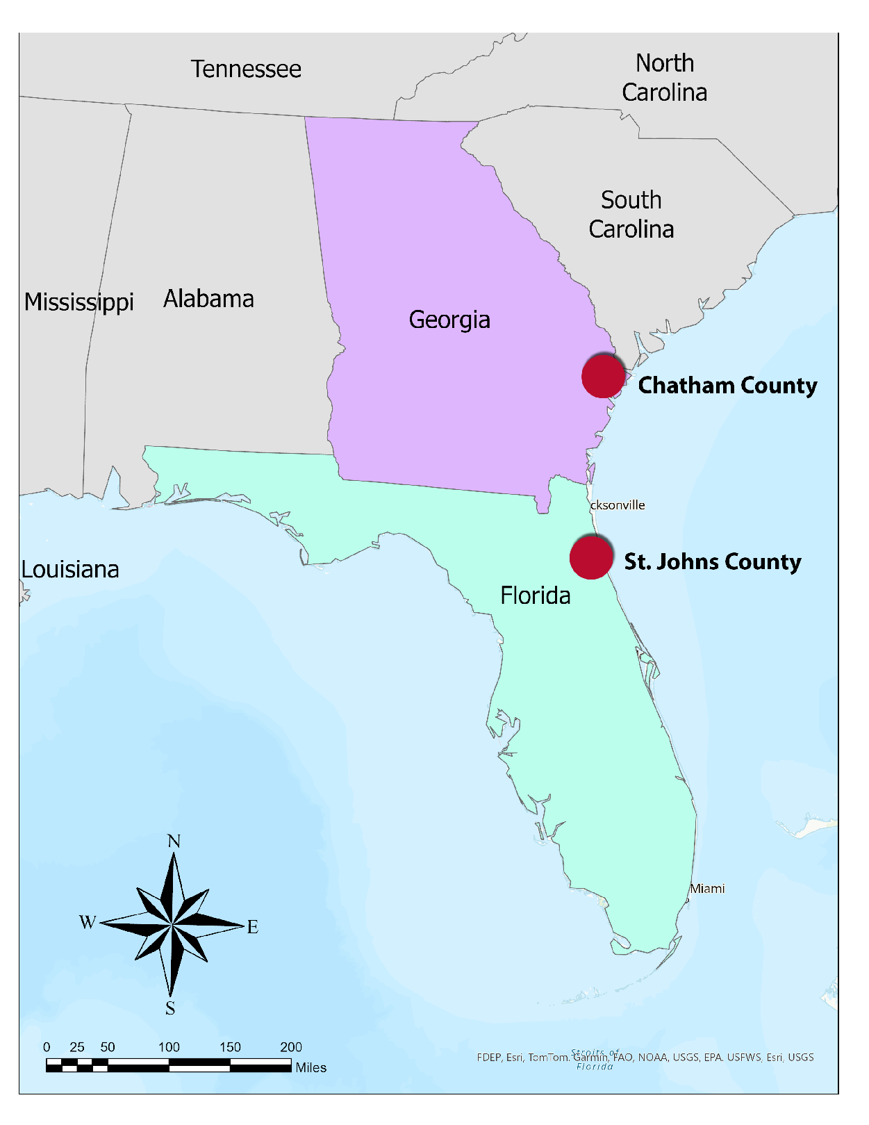
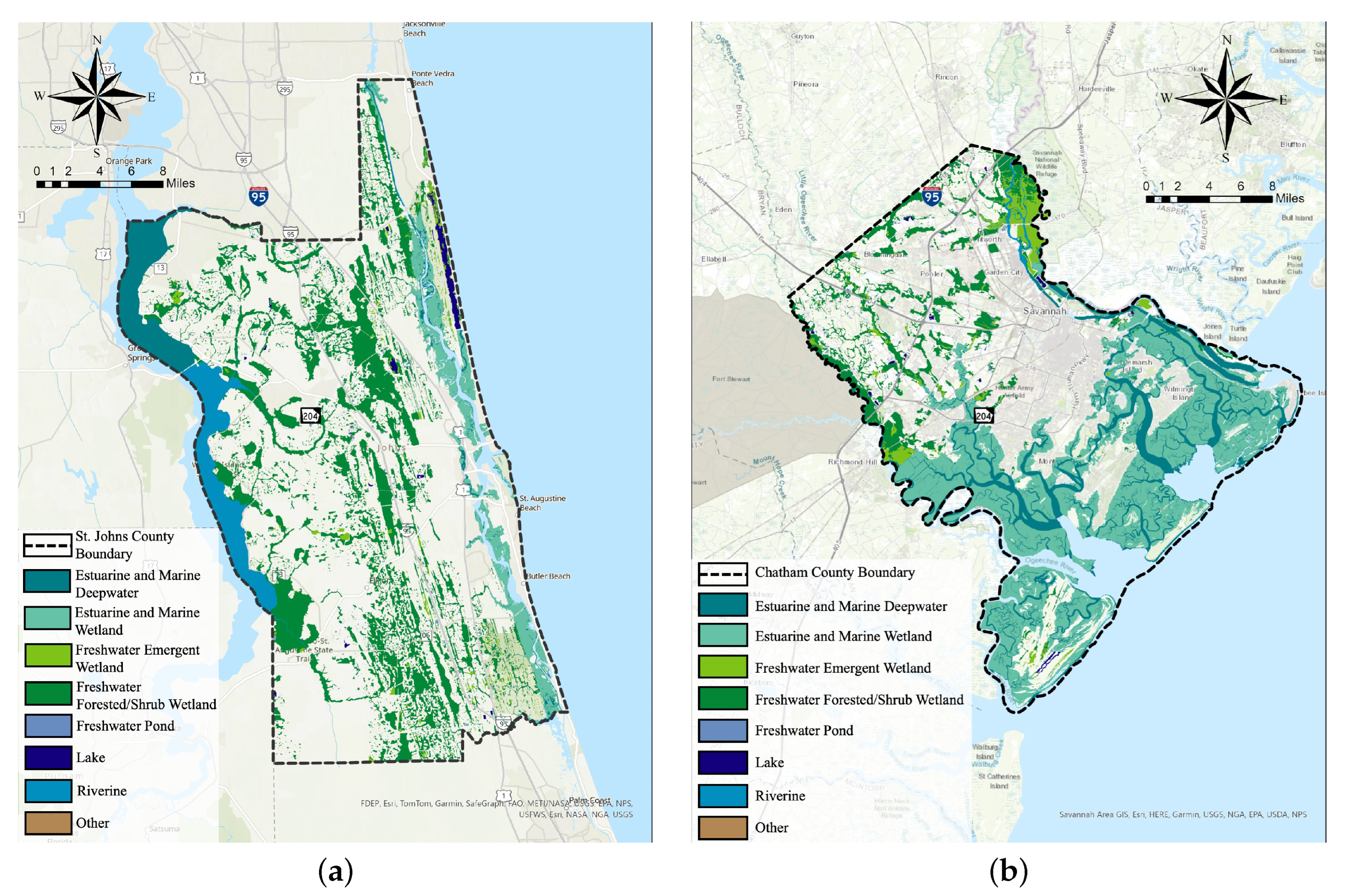
St. Johns County, Florida, and Chatham County, Georgia, both located along the southeast coast of the United States, are the study areas for this research (Figure 1). They are recognized as historical cities in strategic locations that date back to the foundation of the United States in the 18th century. Meanwhile, according to the National Wetlands Inventory and Intact Habitat Cores data, created as part of Esri’s Green Infrastructure Initiative, both counties have large areas of wetlands as part of their core habitats (52% in St. Johns County and 77% in Chatham County).
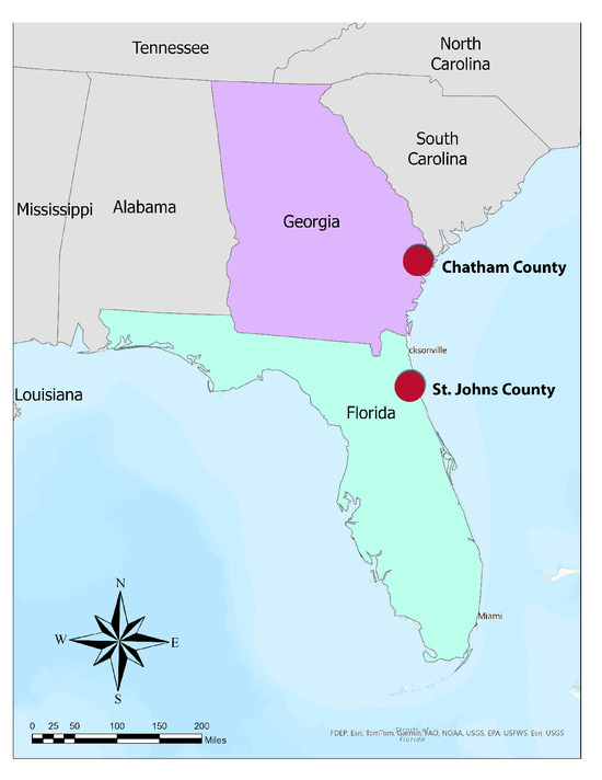
Figure 1.
Study areas: Chatham County and St. Johns County in the southeastern United States.
The city of St. Augustine in St. Johns County, Florida was founded in 1565 by Spanish colonists, and it is recognized as the United States’ oldest continuously inhabited settlement, with a heritage spanning Native American, European, and African-American origins [37]. With consideration for defense and security, the urban area was built closer to the ocean, and there is a barrier island (Anastasia Island) that protects the city’s downtown. Therefore, the city is more vulnerable to SLR due to its location. St. Augustine was established with two objectives: functioning as a military outpost to defend Florida and serving as a hub for the establishment of Catholic missionary settlements [38]. The Spanish colonists emphasized town planning, and the architecture has been inspired by Spanish-Floridian culture for a long time. In the present day, the city is undergoing rapid growth and experiencing changes in land use, driven by the expansion of Jacksonville (about 50 miles north of St. Augustine) into this region.
Savannah, the oldest city in Georgia, was founded by British colonists in 1733. The Oglethorpe Plan, which was conceived by Georgia’s founder James Oglethorpe (1696–1785), was intended to offer a new start for England’s working poor and to strengthen the colonies by increasing trade [39]. The urban area was located on higher elevations along the Savannah River, which provided access to the Atlantic Ocean and facilitated trade and transportation. The city was planned on an agrarian model of sustenance while sustaining egalitarian values and trying to provide equal access to lands. In addition to the city area, large areas of protected coastal marsh, thanks to the Marshland Protection Act, enacted in 1970 [40], act as a buffer zone in the eastern portion of the county for alleviating the impact of SLR. Currently, the growth of the city is occurring towards the western inland counties, a trend that is expected to intensify further. This is attributed to the upcoming Hyundai EV plant construction in Bryan County and the expansion of warehouses and industrial facilities driven by the Port of Savannah.
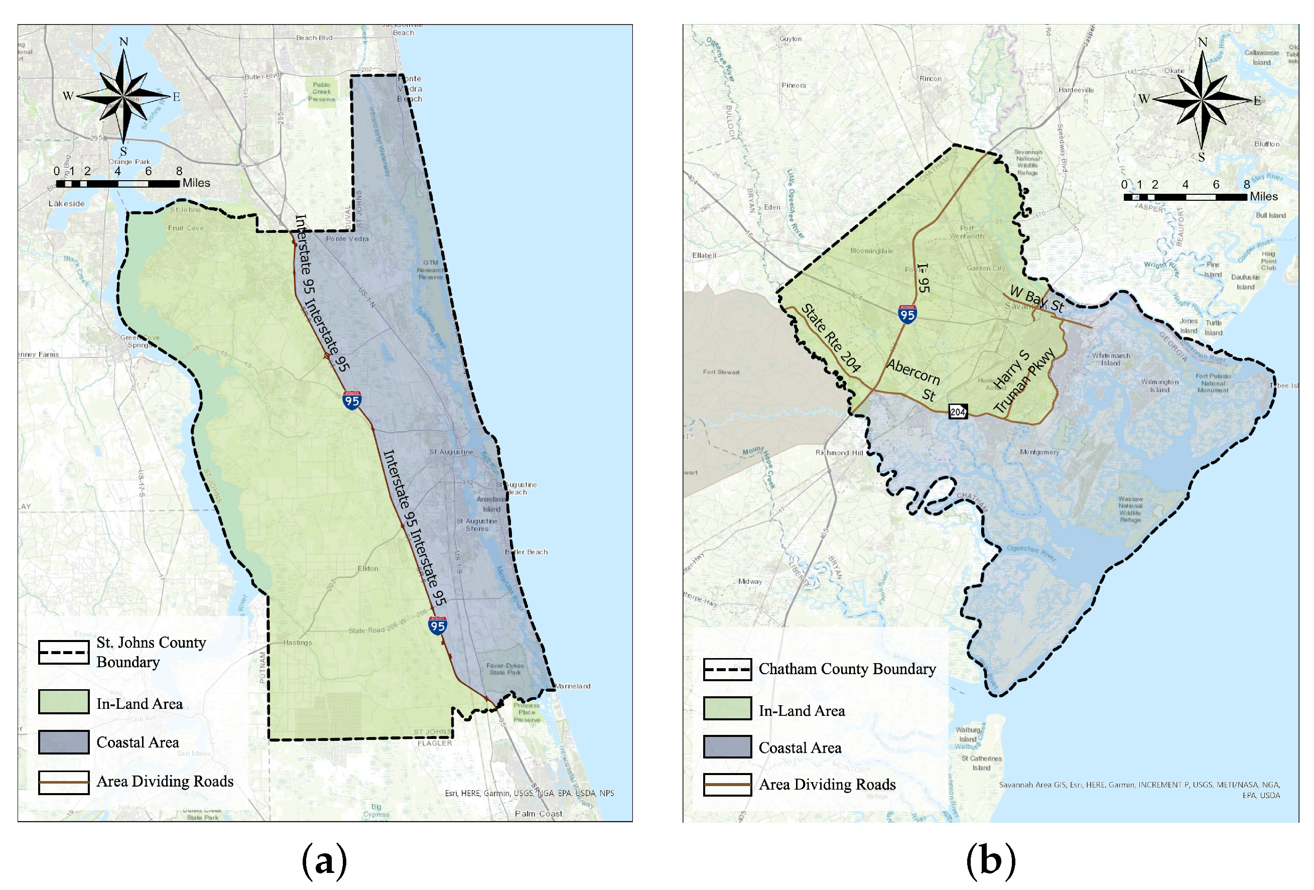
For the purpose of this study, and to establish a clear boundary to compare the difference between the inland and the ocean area, each county was divided into two parts, based on the transportation system (Figure 2).
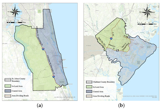
Figure 2.
Study area boundaries established for this study, based on existing transportation systems: the coastal area and the inland area. (a) St. Johns County. (b) Chatham County.
The I-95 highway serves as the dividing boundary for St. Johns County, whereas, for Chatham County, the dividing line also encompasses sections of I-95, in addition to State Route 204, Harry S Truman Parkway, and US Highway 17. In St. Johns County, the inland area is 1017.1 km2, and the coastal area is 726.8 km2. St. Augustine, the city is located near the coastal area. In Chatham County, the inland area is 560.7 km2, while the coastal area is 794.4 km2. Most of the urban built area, including Savannah City, is located on the inland side.
3.2. Data Resources and Landscape Metrics
Datasets used in this study included the Intact Habitat Cores data (created as part of Esri’s Green Infrastructure Initiative), the SLR data provided by NOAA (National Oceanic and Atmospheric Administration), and 10 m land-cover time series of the world based on Sentinel-2 imagery from 2017–2020, produced by Impact Observatory, Microsoft, and Esri. The Intact Habitat Cores data identified the most valuable landscapes before growth and development began in the U.S. It was derived using a combination of the U.S. Geological Survey National Land-Cover Database and the U.S. Census Bureau’s TIGER files for roads and railroads. The methodology was based on Evaluation and Conserving Green Infrastructure Across the Landscape: A Practitioner’s Guide [41]. Core habitats in this study were identified based on this dataset. High-resolution 10 m land-cover time series maps, which are open, accurate, and comparable, were applied to analyze changes in urban built areas. These maps provide a 9-class classification of the surface, including vegetation types, bare surfaces, water, cropland, and built areas. For the landscape and urban change studies, the core habitats and urban built areas were identified as patches, a landscape ecology unit that describes discrete communities or species assemblages surrounded by an area of dissimilar community structure or composition [42]. For the landscape and urban metrics, there are 12 metrics used in this paper in total. Half of these metrics [43] are selected for measuring the core habitats (Table 2), while the other half are selected for measuring urban built area change, especially focusing on assessing spatial characteristics of land-use and urban structure change with sea level rising (Table 3).
Table 2.
Metric selection for core habitats.
Table 3.
Metric selection for urban built area change.
The percent of landscape (PLAND) metric was used to quantify the abundance of urban green infrastructure. Cities with larger PLAND values have more green infrastructure. Largest patch index (LPI) was used to measure the dominance of urban green infrastructure in the landscape. Large LPI values mean that the largest urban green patch is more dominant in cities. Patch density (PD) was used to quantify the fragmentation of urban green infrastructure. Cities with larger PD values have more fragmented urban green infrastructure. Mean Euclidean nearest-neighbor distance (ENN_MN) was used to quantify the isolation of urban green patches. As the patch type becomes more aggregated, the percentage of like adjacencies (PLADJ) metric increases, indicating a higher proportion of like adjacencies [44].
The number of urban patches (NP) and the PD evaluate the change in urban patches, with NP and PD being high when there is growth in subdivided urban areas. This may indicate rising sea levels, leading to the fragmentation of urban patches. The largest patch index (LPI) represents the percentage of an urban core area as a proportion of total urban land, and the LPI decreases when the urban areas become more dispersed. The area-weighted mean patch fractal dimension (FRAC_AM) is a measure of patch shape complexity. The FRAC_AM metric approaches 1 for shapes with very simple perimeters such as circles or squares and approaches 2 for shapes with highly convoluted, plane-filling perimeters [45].
3.3. Methods
3.3.1. Core Habitats Identification
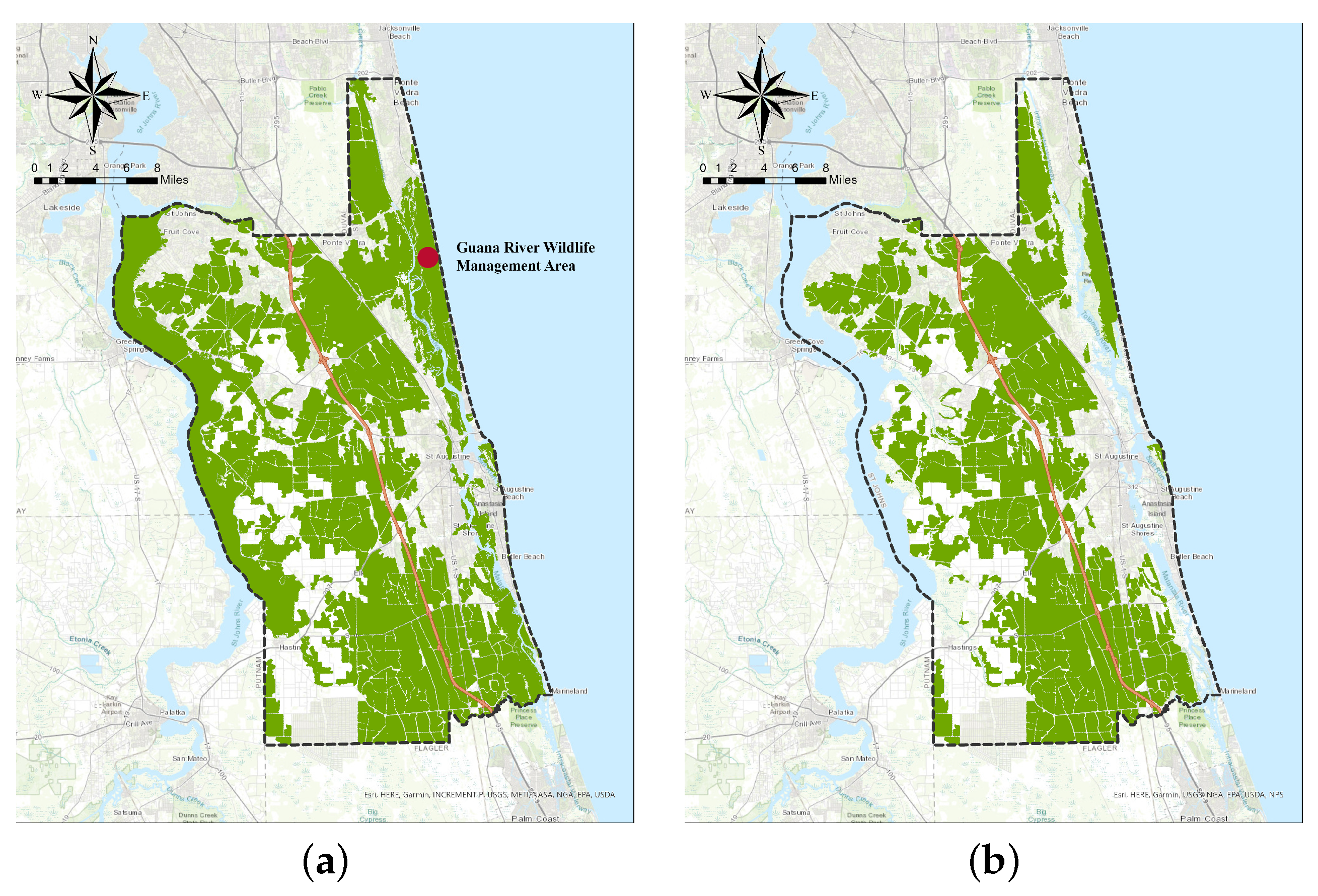
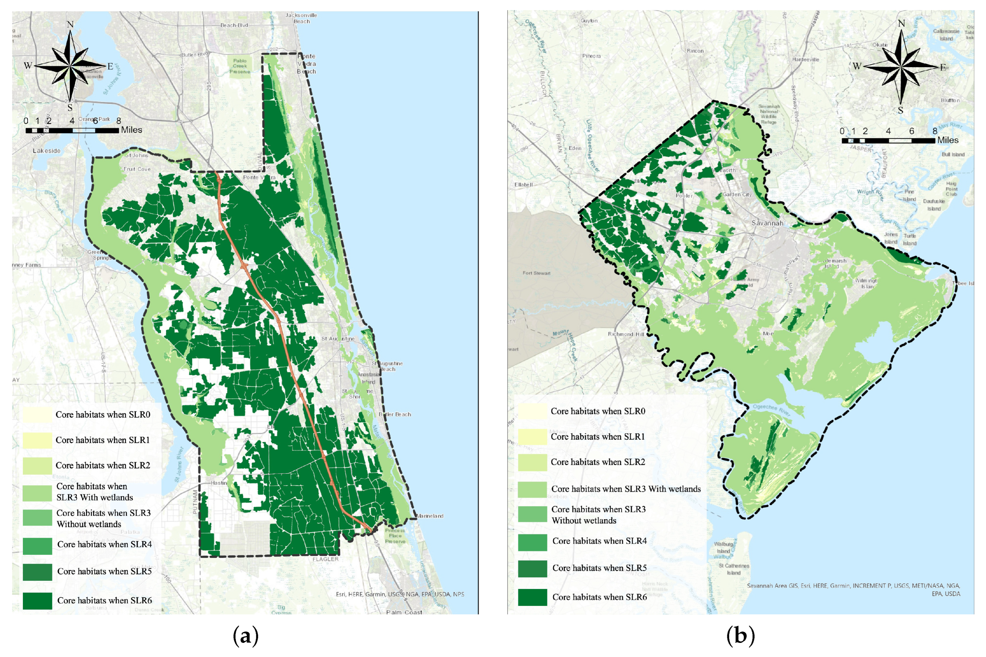
The concept of core habitats applied in this paper is an area or patch of relatively intact habitat that is sufficiently large to support more than one individual of a species. In 2015, the Green Infrastructure Center published a methodology implemented by ArcGIS Toolboxes. The methodology defined cores with larger volumes, and smaller perimeters have more interior habitats than those that are long and thin. In general, areas with water bodies, perennial streams and rivers, and wetlands are preferred [46]. The definition of core habitat, in this case, should be a minimum of 100 acres (40.5 ha) and a width of 200 m. According to this definition, we identified the core habitats with wetlands (Figure 3) together in each foot of the SLR scenario. We then refined the selection to include only core habitats that measured 100 acres or more. Commonly, the connectivity and biodiversity of core habitats are susceptible to the impacts of SLR. Under typical circumstances, wetland core habitats possess a natural capacity to adjust to changing sea levels [24]. They can adapt through mechanisms, such as sedimentation, vertical accretion, or migration inland. However, if SLR occurs at a rate that exceeds the wetlands’ ability to adapt, this may result in the inundation of these habitats.
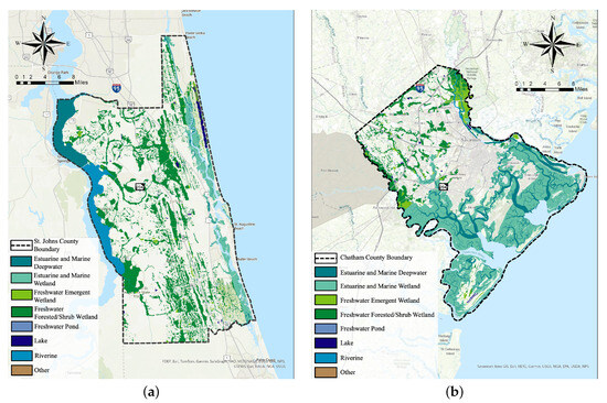
Figure 3.
Wetland core habitats in both counties. (a) St. Johns County core wetlands. (b) Chatham County core wetlands.
In five numerical models [7,8,9,10,11] investigating the long-term evolution of coastal marshland, results have shown that, once a certain SLR rate threshold is exceeded, inundation leads to the irreversible transformation of intertidal marshland into unvegetated areas. In such a scenario, these areas can no longer be considered as core habitats. The consensus among these models is that, by approximately the year 2080, accretion rates will decline to a level where sustaining vegetation is no longer possible [12]. In this study, the local intermediate SLR around the year 2080 would be 2.56 feet (Table 1). Therefore, two scenarios were considered for an SLR of 3 feet. The first scenario incorporates inundated wetlands as part of the core habitats, whereas the second scenario excludes them.
In this paper, two workflows were created for core habitat identification:
- For core habitats when SLR is lower than 3 feet: (1) Select the wetlands classified as core habitats. (2) Integrate the core wetlands with other core areas that are not susceptible to ocean submersion. (3) Identify remaining areas that are capable of meeting the “core habitat” criteria. (4) Incorporate maps into FRAGSTATS [13] and perform metric calculations;
- For core habitats when SLR is higher than 3 feet: (1) Identify core habitats unaffected by SLR. (2) Integrate maps into FRAGSTATS [13] and compute relevant metrics.
3.3.2. Mapping Urban and Landscape Changes under SLR Scenarios
Two general maps were produced to show the core habitats’ change from SLR 0 to 6 feet and the urban built area change from SLR 0 to 7 feet. We examined eight scenarios for both changes in core habitat and urban built areas. Specifically, regarding core habitat change, two scenarios were considered, corresponding to an SLR of 3 feet. The quantity and scale were compared in Table 4 and Table 5 to clearly describe the habitats lost by SLR. Moreover, three areas with the most dramatic changes in each county were selected for more detailed analysis, including morphological changes and inferences about causes. For SLR at 3 feet, 2 different scenarios were mapped due to wetlands resilience, as described in Section 3.3.1. To facilitate a clear depiction of landscape changes on the maps, SLR scenarios ranging from 0 to 2 feet are combined, as are scenarios from 4 to 6 feet. Meanwhile, for urban built area change, sea level rise scenarios ranging from 0 to 3 feet are combined, as are scenarios from 4 to 7 feet.
Table 4.
Green infrastructure identification for SLR from 0 to 6 feet in St. Johns County.
Table 5.
Green infrastructure identification for SLR from 0 to 6 feet in Chatham County.
3.3.3. Quantifying Urban and Landscape Change by Metrics
The exported raster data of urban built areas and core habitats in each SLR scenario were imported into FRAGSTATS [13] to calculate the landscape metrics. The outputs were compared between the two study areas.
4. Results
4.1. Core Habitats Identification
4.1.1. St. Johns County Core Habitat Identification
Eight maps of core habitats that would remain after SLR of 0 to 6 feet were generated and overlapped to identify where significant changes would occur (Appendix A, Figure A1). When SLR in St. Johns County ranges from 0 to 3 feet, the areas with more drastic changes are mainly located in the peripheral areas (Figure 4). In addition to water from the ocean, the water from the St. Johns River would impact the core habitats from the west. Therefore, the increase in sea level from 0 to 2 feet results in a reduction of 8 km2 in the area of the core habitat (Table 4).
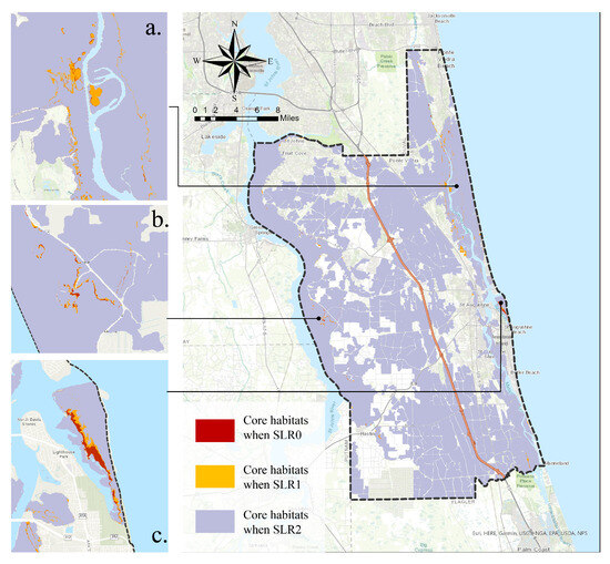
Figure 4.
Overlapped maps of core habitats remaining when SLR transitions from 0 to 2 feet in St. Johns County. (a–c) are detailed maps of sites with significant reductions in core habitats.
For the two scenarios when the sea level rises 3 feet, both are highly impacted by the SLR. In the SLR of 3 feet scenario that includes the wetlands, the area of core habitats is reduced by 9.8 km2 compared to SLR of 2 feet. For the scenario that did not include wetlands, the core habitats would only be 800.4 km2, which is reduced by 280.5 km2 compared to SLR of 2 feet (Table 4). Inundated core habitats are mainly located along the bank of St. Johns River and along the coastline (Figure 5).
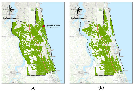
Figure 5.
The maps of remaining core habitats with SLR at 3 feet in St. Johns County. (a) With wetlands. (b) Without wetlands.
When the sea level rises from 4 to 6 feet (Figure 6), the area of remaining core habitats would be around 752 km2. Much of the core habitat in the Guana River Wildlife Management Area (red dot in Figure 5a and enlarged area in Figure 6a) would be flooded. In the meantime, the number of core habitats remained relatively stable during that period (148 when SLR was at 0 feet and 147 when SLR was at 6 feet), which means that the remaining habitat patches would become smaller and more isolated from each other. This isolation would contribute to increased fragmentation.
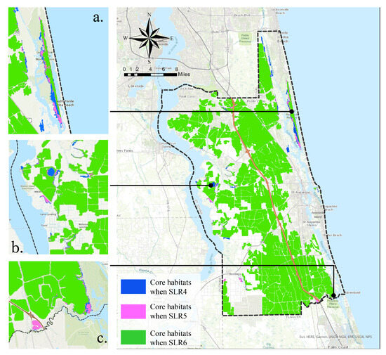
Figure 6.
Overlapped maps of core habitats remaining when SLR transitions from 4 to 6 feet in St. Johns County. (a–c) are detailed maps of sites with significant reductions in core habitats.
4.1.2. Chatham County Core Habitat Identification
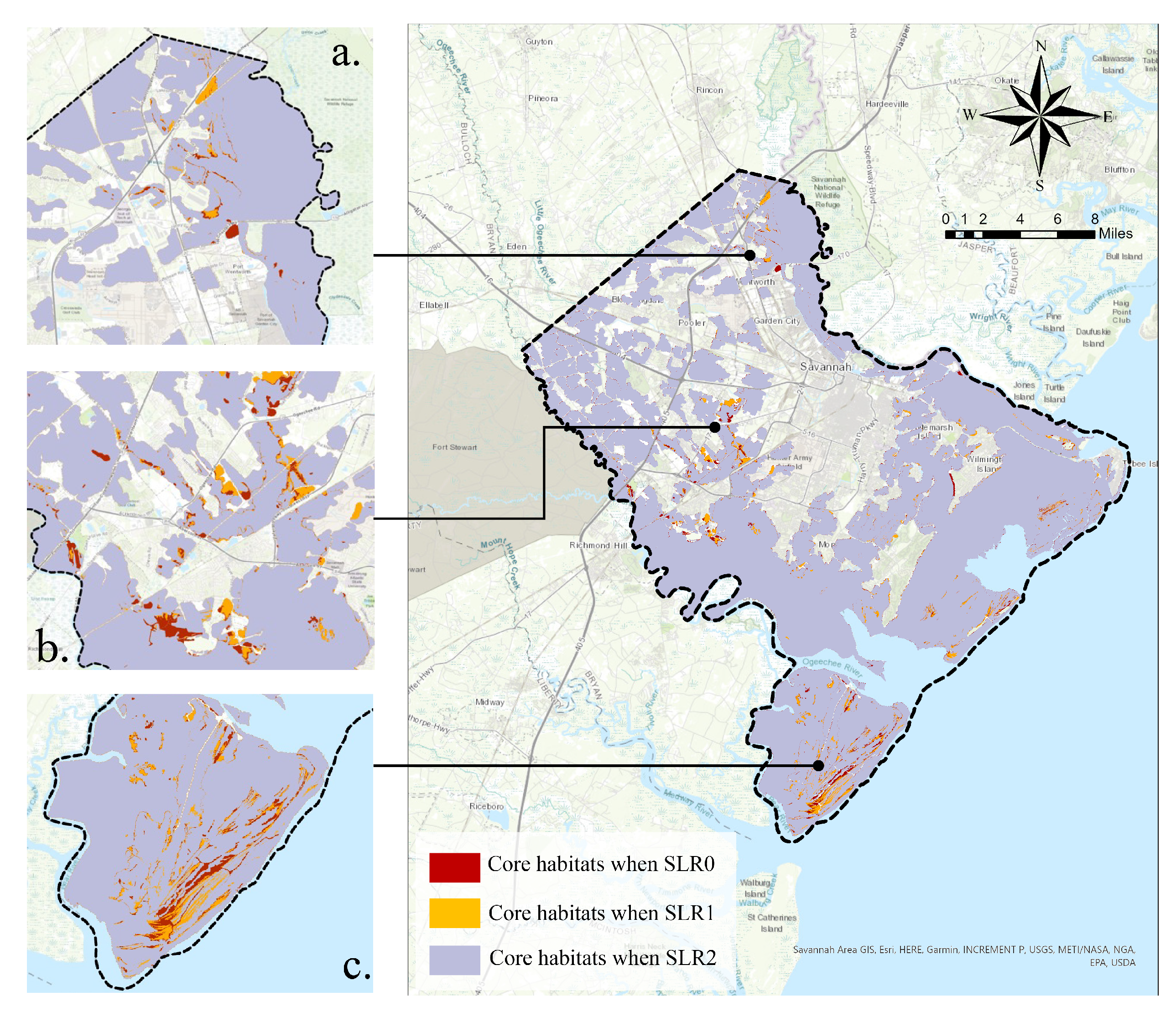
With SLR at 0 feet, there are a total of 78 core habitats, totaling 822.4 km2 in Chatham County. As the sea level rises, the number of core habitats is slowly increasing but the areas are decreasing dramatically, which means that it is possible that the degree of fragmentation of core habits is becoming higher and higher. Similar to the workflow in St. Johns County, eight output maps of core habitats that remained after SLR of 0 to 6 feet were also generated and overlapped to identify where significant changes would occur (Appendix A, Figure A2).
When SLR is from 0 to 2 feet (Figure 7), there is a reduction of 36.6 km2 in the area of the core habitat (Table 5). The area most affected by this process is the Ossabaw Island Wildlife Management Area, which is located in the south part of the county (Figure 7c). The reduction of core habitats in the southwestern region due to the impact of the Little Ogeechee River is also significant in this process.

Figure 7.
Overlapped maps of core habitats remaining when SLR transitions from 0 to 2 feet in Chatham County. (a–c) are detailed maps of sites with significant reductions in core habitats.
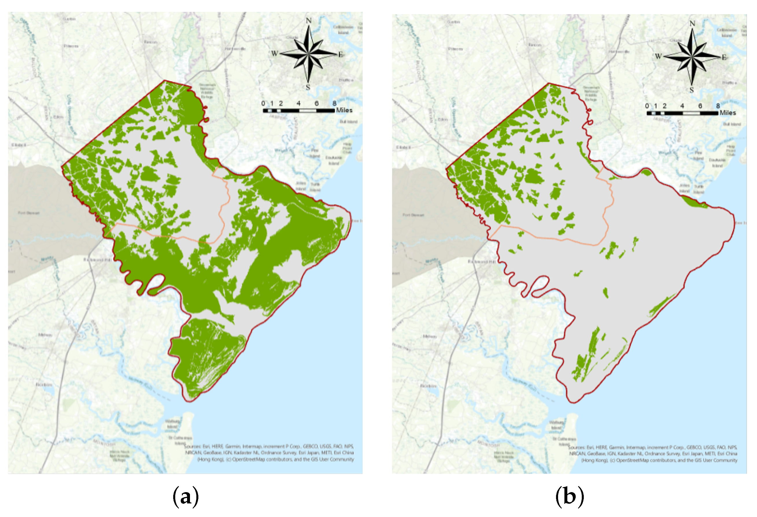
The presence of extensive wetlands in the eastern region of Chatham County led to two distinct outcomes for the scenarios when SLR reached 3 feet (Figure 8). With wetlands, the area of core habitats is 768.9 km2, while, without wetlands, the area is only 191.1 km2 (Table 5). In contrast to the significant decrease in the area, the number of core habitats has increased from 81 to 83 with wetlands and 94 without wetlands. This is because fragmentation leads to a decrease in the overall area of each core habitat while simultaneously increasing the number of fragmented patches. Core habitats became smaller and more isolated. The core habitats in the east and south are almost completely flooded and can no longer provide survival protection for wildlife. The main ecological network of the entire county will be relocated to the northern interior part.

Figure 8.
The maps of remaining core habitats with SLR at 3 feet in Chatham County. (a) With wetlands. (b) Without wetlands.
However, with SLR from 4 to 6 feet (Figure 9), even inland ecological networks could be affected by rising sea levels. Part of the core habitats in the north near the county boundary line will be inundated by water. In this process, nearly 24 km2 of core habitats will be lost.
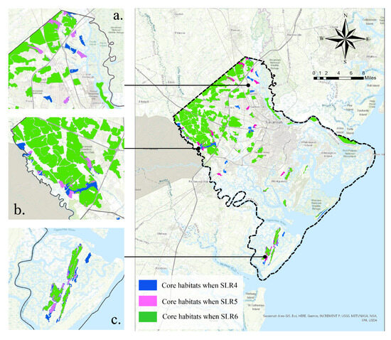
Figure 9.
Overlapped maps of core habitats remaining when SLR transition from 4 to 6 feet in Chatham County. (a–c) are detailed maps of sites with significant reductions in core habitats.
4.1.3. Comparison of Landscape Metric Changes between the Two Counties
Both counties are divided into inland and coastal areas. In St. Johns County, both areas are highly influenced by SLR. Figure 10 depicts the values of different landscape metrics for the west and east subareas of St. Johns and Chatham Counties as histograms, for different levels of SLR, with and without wetlands. From the graphs, the variation curves of NP, PLAND, PD, and mean patch shape index (SHAPE_MN) are relatively similar in terms of inland and coastal areas. For ENN_MN and PLADJ, when SLR is at 3 feet, the changes start to become drastic, especially in the east area, which is close to the ocean. The ENN_MN is calculated as the straight-line distance between the centroids of the two patches. According to the graphs, it can be noticed that the distances between each pair of core habitats increase with higher SLR in the west and decrease in the east region in St. Johns County. Both regions’ PLADJ values decrease with higher SLR, which means less even distribution of patch sizes and, therefore, less diversity. In Chatham County, it is obvious that landscape metrics in areas near the ocean change more dramatically than inland areas. Low-lying coastal areas are more susceptible to being submerged as SLR increases. This inundation can lead to the loss of valuable land, causing changes in landscape metrics values. Due to the reduction of core habitats, the PLAND value of the area near the ocean drops sharply after SLR of 3 feet (from 27.4 to 1.7), and the Euclidean distance between the habitats increases (from 24.1 to 558.8). Research conducted in the Atlantic Forest and Cerrado of Brazil indicates that relatively small distances between habitat fragments, ranging from 100 to 500 m, can function as barriers for certain species [47]. As a result, the Euclidean distance between habitats in this study has decreased to a point where it scarcely meets the migratory needs of some wildlife species.
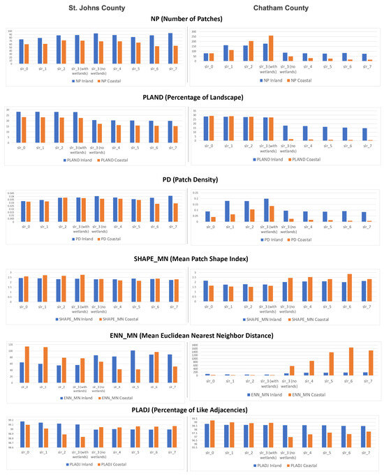
Figure 10.
Comparison of landscape metrics change for core habitats between the two counties. Histograms depict landscape metrics computed for inland and coastal areas at different SLR levels. On the left side are the calculated landscape metric results for St. Johns County, while the right side displays the landscape metric results for Chatham County.
4.2. Urban Built Area Change Identification
4.2.1. St. Johns County Urban Built Area
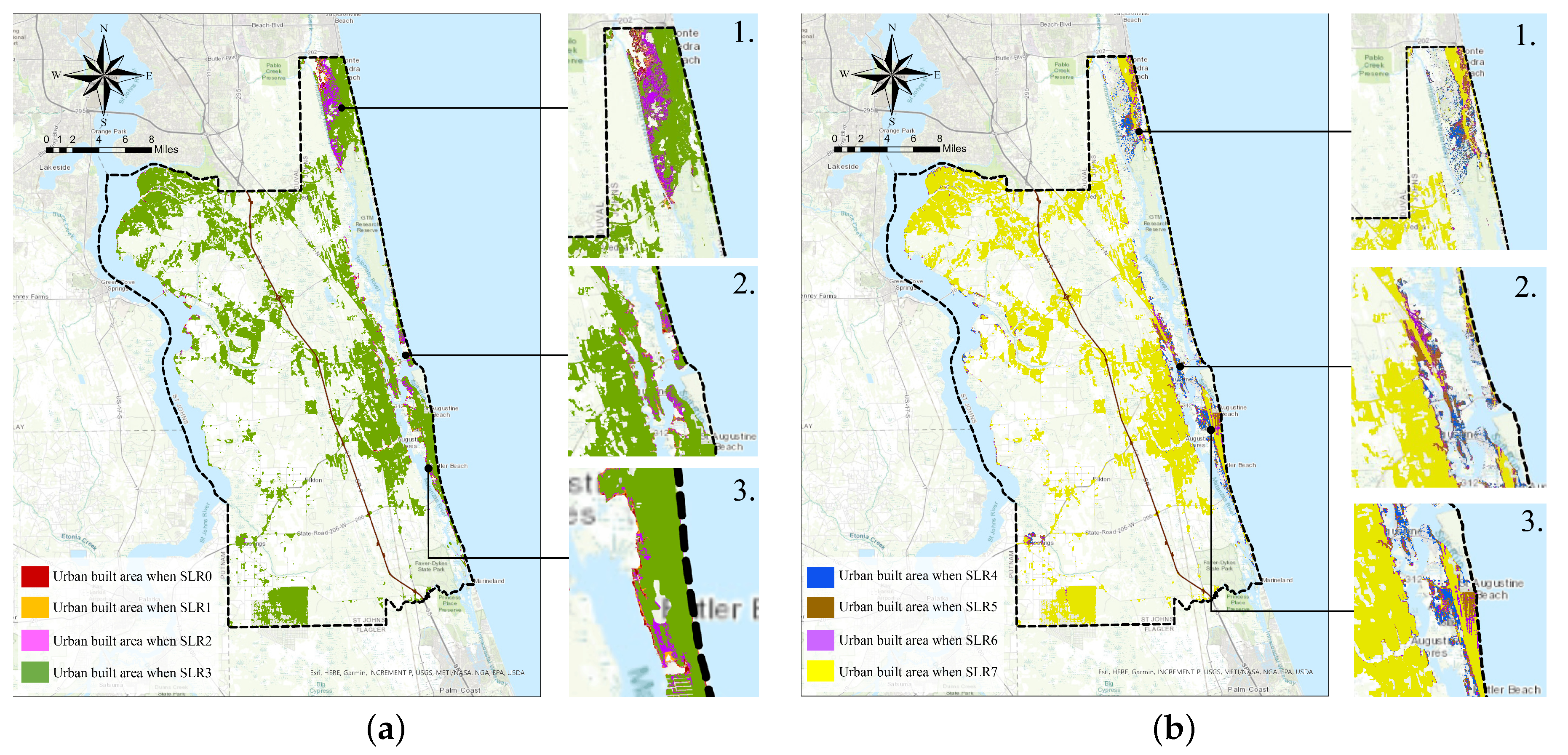
For measuring the urban built area change, eight output maps of the remaining urban built area with SLR of 0 to 7 feet were generated and overlapped to identify where significant changes would occur (Appendix A, Figure A3). St. Augustine is in the east area of St. Johns County. Most of the urban built areas in this county are along the coastline, which means that they will be more vulnerable when sea level rises. From SLR 0 to 4, the most vulnerable areas are Palm Valley and the areas near Matanzas River and Salt Run in St. Augustine (Figure 11). The situation will become worse when SLR reaches 7 feet and the built area in St. Augustine will be almost completely submerged. The built areas in this county are less protected by wetlands; therefore, when the sea level rises, the city areas will have less buffer from rising sea levels.
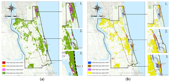
Figure 11.
Overlapped maps of urban built areas remaining in St. Johns County. (a) SLR transitions from 0 to 3 feet. (b) SLR transitions from 4 to 7 feet. (1), (2), and (3) are detailed maps of sites with significant reductions in urban built area.
4.2.2. Chatham County Urban Built Area
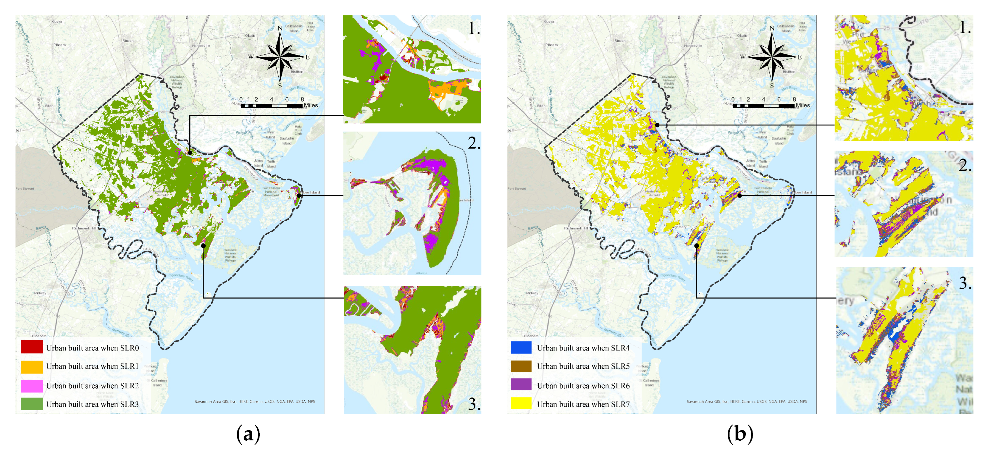
Eight output maps of the remaining urban built area with SLR of 0 to 7 feet were also generated and overlapped to identify where significant changes would occur in Chatham County (Appendix A, Figure A4). The impacts of SLR on core habitats and urban development in Chatham County may not be as severe because Savannah and its surrounding areas have more elevated areas and coastal marshes to buffer the rising ocean. From SLR 0 to 4 feet, the most affected areas are Skidaway Island, Wilmington Island, Tybee Island, and some areas along the Savannah River (Figure 12). As the county seat, Savannah shows less impact due to its location on higher terrain and the large areas of wetland as buffer zones in comparison with St. Augustine in St. Johns County. Even if the SLR reaches 7 feet, the region along the river would still experience the greatest impact, while other areas would remain comparatively secure.

Figure 12.
Overlapped maps of urban built areas remaining in Chatham County. (a) SLR transitions from 0 to 3 feet. (b) SLR transitions from 4 to 7 feet. (1), (2), and (3) are detailed maps of sites with significant reductions in urban built areas.
4.2.3. Comparison of Urban Metric Changes between the Two Counties
In St. Johns County, changes in the values of landscape metrics in the coastal areas are more obvious than in the inland areas (Figure 13). According to the graphics, changes in urban built areas begin to intensify from sea level rise to 3 feet. In the graph of the FRAC_AM, it reaches the highest value when SLR is at 3 feet, which indicates the urban built area with a large proportion of small patches, and could explain why ENN_MN reaches the lowest value at SLR 3 feet. In Chatham County, the value of NP rises while the total area falls, which indicates that the degree of fragmentation is becoming higher. LPI value drops sharply at SLR of 6 feet; this metric calculates the extent to which an area is composed of patches of different sizes. The value shows that the largest built-up urban area (the Savannah city area) is being affected more than ever before by this level of sea level rise.
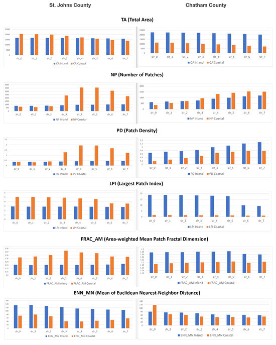
Figure 13.
Comparison of landscape metric changes for urban built areas between the two counties. Histograms depict landscape metrics computed for inland and coastal areas at different SLR levels. On the left side are the calculated landscape metric results for St. Johns County, while the right side displays the landscape metric results for Chatham County.
5. Discussion
5.1. Core Habitat Change in the Two Counties
According to all the metrics, SLR affects the core habitats in the two counties in different ways. In St. Johns, the impact is relatively minor, with a more even distribution between inland and coastal areas (Figure 14). In contrast, in Chatham, the impact is severe, and the trend in core habitat loss is from east to west. Further studies could explore the threshold of wetlands, such as whether the 3-foot threshold applies to other study areas and whether different types of wetlands should be considered. It seems that there is ample room for further exploration of this topic. When the sea level rises to 3 feet, the wetlands experience significant changes, causing most of the landscape metric data to exhibit a drastic decline or increase. Among the core habitats, Chatham County is expected to be more susceptible to the effects of SLR compared to St. Johns County. This is because the majority of the wetlands in Chatham County are concentrated in the low-elevation and ocean-side eastern regions. The NP, PLAND, and PD metrics indicate a sharp decrease in the number of landscape patches, primarily due to the loss of wetlands.

Figure 14.
Core habitat changes in the two counties. (a) St.Johns County. (b) Chatham County.
5.2. Built Area Change in the Two Counties
The maps reveal that the influence of SLR on urban built areas in St. Johns County is more centralized, primarily affecting the northern part and the St. Augustine city area (Figure 15). The northern region happens to be an area of rapid growth and land-use change due to the expansion of Jacksonville towards this area. On the other hand, the impact on Chatham County is more dispersed. The metrics indicate that, as the urban built area diminishes, the number of urban patches increases, especially when the sea level rises from 2 to 3 feet. This suggests that the level of fragmentation in urban built areas progressively increases as the sea level rises. When urban built areas become fragmented, they tend to shrink and become more isolated. This will lead to the loss of green spaces within urban areas and can also exacerbate the urban heat island effect. Urban planning and management will face challenges as fragmented landscapes emerge, characterized by a variety of land ownership patterns and conflicting land uses. The findings indicate that, when the sea level rises to 6 feet, there will be a decrease in the proportion of the largest patches. However, the difference lies in the location where this phenomenon occurs, with the inland area of Chatham County and the coastal area of St. Johns County being affected. This pattern aligns with the original construction layout in the two counties’ history, as St. Johns County’s urban areas have their origins in offshore regions, whereas Chatham County’s origins trace back to inland areas. Despite the impact of rising sea levels, the shape of the urban patches remains relatively uniform and symmetrical.
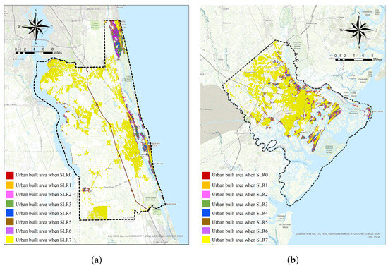
Figure 15.
Urban built area changes in the two counties. (a) St. Johns County. (b) Chatham County.
Researchers have characterized long-term trends and patterns in land-cover change based on landscape metrics [48], and most of them have utilized data from within the past 50 years [49,50,51]. They commonly explore urban and natural landscapes as distinct systems. And they either apply landscape metrics for urban sprawl and growth [52,53] or monitored landscape change specifically [54]. In this study, not only long-time future SLR projections according to NOAA (a nearly 100-year span) were utilized, but also both natural wetland landscapes and urban built area changes caused by SLR. Studying the two systems simultaneously allows for a holistic understanding of the interactions between urban and natural environments. Moreover, learning about urban and landscape changes provides insights into how land-use decisions can balance the needs of development with the preservation of natural coastal features.
In St. Johns County, as the threat of rising sea levels encroaches from both the eastern and western edges of the county towards the center, urban and landscape planning will need to adapt to the evolving land-use patterns in the diminishing space. In contrast to Chatham County, St. Augustine and other cities in Florida, including Jacksonville and other nearby urban areas, are growing at an accelerated pace (faster than Georgia coastal cities) and, therefore, face more pressing demands for population and property relocation. In Chatham County, with the increasing sea levels and the city’s expansion towards the west, forthcoming landscape and urban planning priorities will pivot towards the northwest and west of the county. Achieving balanced development, which involves planning urban spaces while preserving core habitats and landscape connectivity, becomes crucial in making informed planning decisions.
Given the study’s specific focus on the integrated changes in urban and natural landscapes when SLR ranged from 0 to 7 feet, the sample size was necessarily restricted and statistical tests were not conducted because the analysis was based only on observed trends. However, in forthcoming research endeavors, we intend to expand the sample size, for example, to evaluate the changing trend comparison between each patch and to implement statistical analyses to augment the validity and reliability of our findings, thereby ensuring a more comprehensive understanding of the SLR impacts.
6. Conclusions
Utilizing up-to-date and high-resolution remote sensing data and geospatial predictions of localized SLR data, the geospatial analyses, maps, and landscape metrics presented in this study offer an optimal foundation for urban coastal and landscape planning. Furthermore, incorporating urban and landscape metrics into SLR studies can provide valuable insights and enhance the understanding of how coastal cities might respond to rising sea levels. Overall, assessing local changes in predicted impacts of SLR on landscapes and urban development can serve as a foundation for designing and implementing effective strategies, enabling us to respond to the challenges posed by rising sea levels with greater confidence and efficiency.
Author Contributions
Conceptualization, J.Z., R.G.R. and M.M.; methodology, J.Z. and R.G.R.; software, J.Z.; validation, J.Z.; formal analysis, J.Z.; investigation, J.Z.; resources, J.Z. and M.M.; data curation, J.Z.; writing—original draft preparation, J.Z.; writing—review and editing, J.Z., R.G.R. and M.M.; visualization, J.Z.; supervision, R.G.R. and M.M. All authors have read and agreed to the published version of the manuscript.
Funding
This research received no external funding.
Institutional Review Board Statement
Not applicable.
Informed Consent Statement
Not applicable.
Data Availability Statement
Due to the nature of the research, data that support the findings of this study are not available. The data used to generate our findings are available upon request from the corresponding author.
Conflicts of Interest
The authors declare no conflicts of interest.
Abbreviations
The following abbreviations are used in this manuscript:
| ENN_MN | Mean Euclidean nearest-neighbor distance |
| FRAC_AM | Area-weighted mean patch fractal dimension |
| GMSL | Global Mean Sea Level |
| LPI | Largest patch index |
| MDPI | Multidisciplinary Digital Publishing Institute |
| NOAA | National Oceanic and Atmospheric Administration |
| NP | Number of patches |
| PD | Patch density |
| PLADJ | Percentage of like adjacencies |
| PLAND | Percentage of landscape |
| SHAPE_MN | Mean patch shape index |
| SLR | Sea level rise |
| TA | Total area |
Appendix A

Figure A1.
Remaining core habitat maps when SLR transitions from 0 to 6 feet in St. Johns County.
Figure A1.
Remaining core habitat maps when SLR transitions from 0 to 6 feet in St. Johns County.
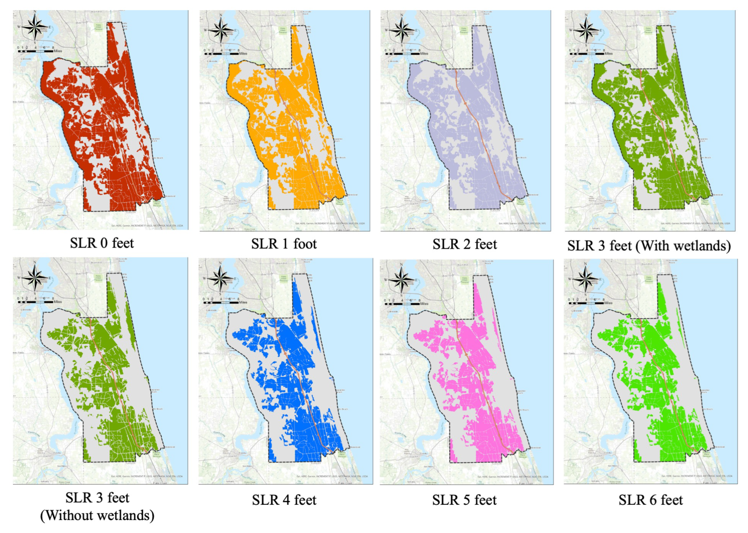
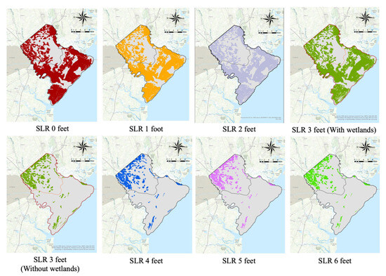
Figure A2.
Remaining core habitat maps when SLR transitions from 0 to 6 feet in Chatham County.
Figure A2.
Remaining core habitat maps when SLR transitions from 0 to 6 feet in Chatham County.
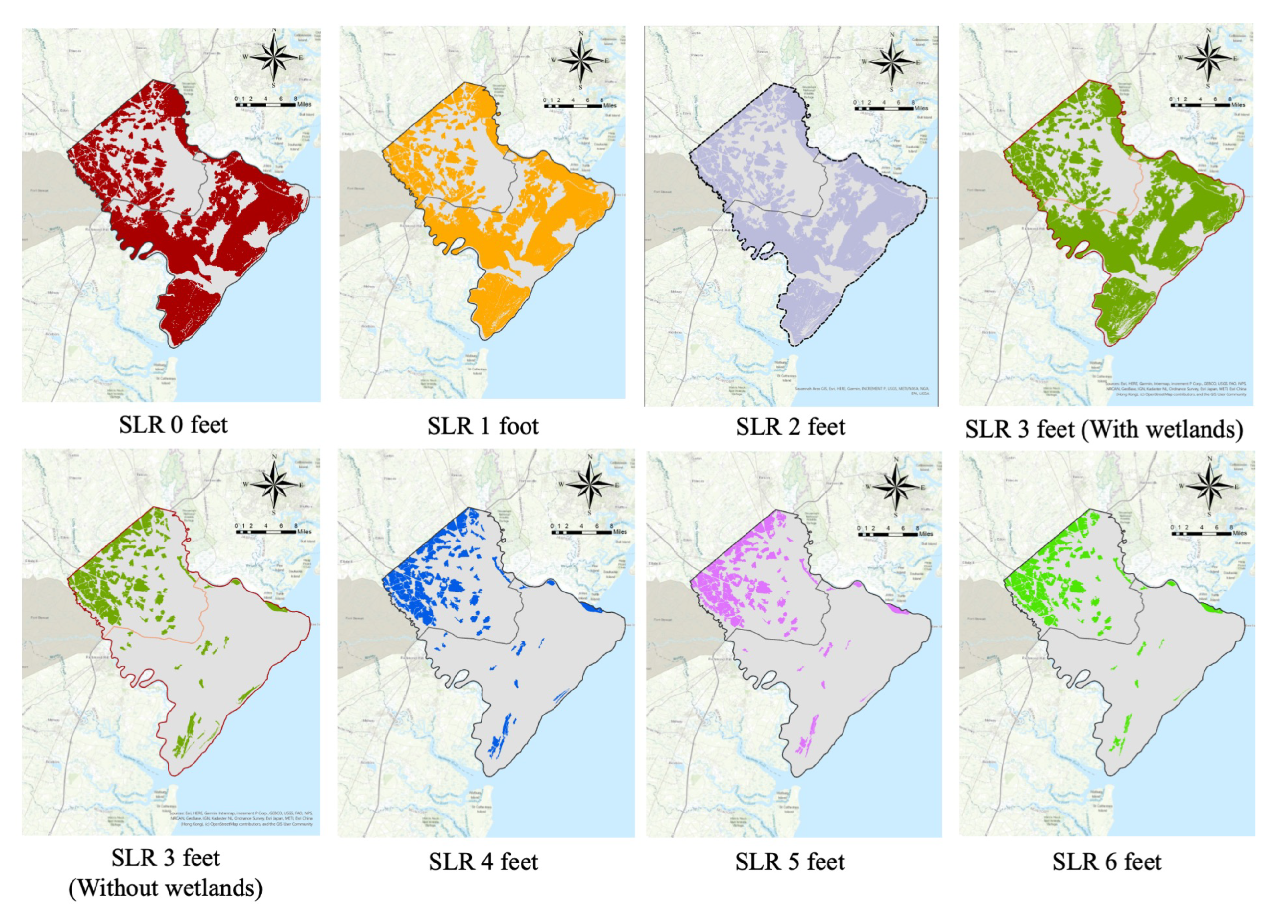
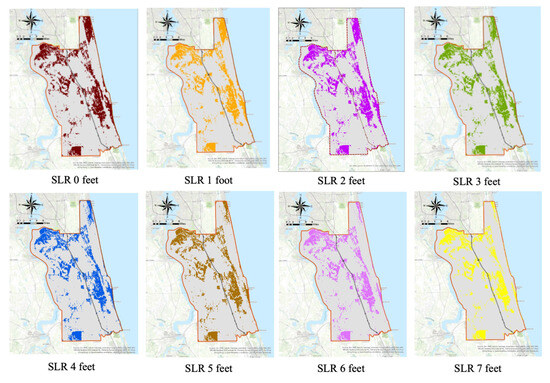
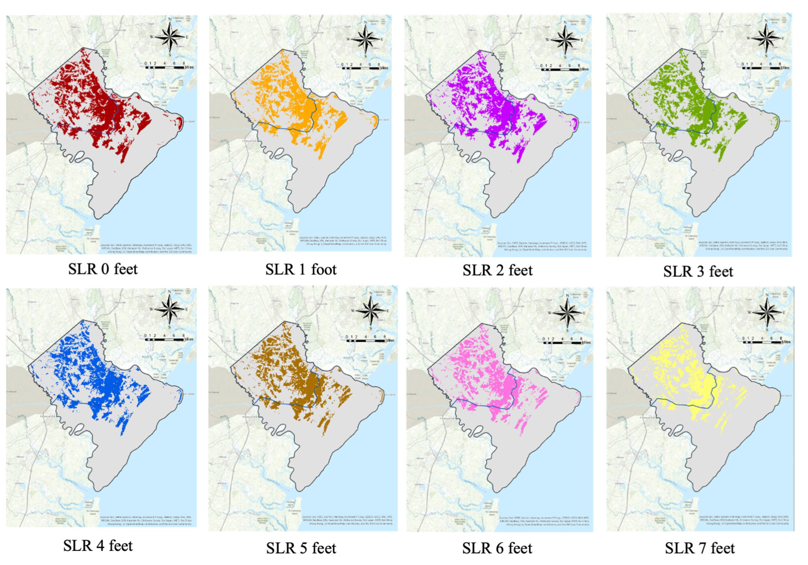
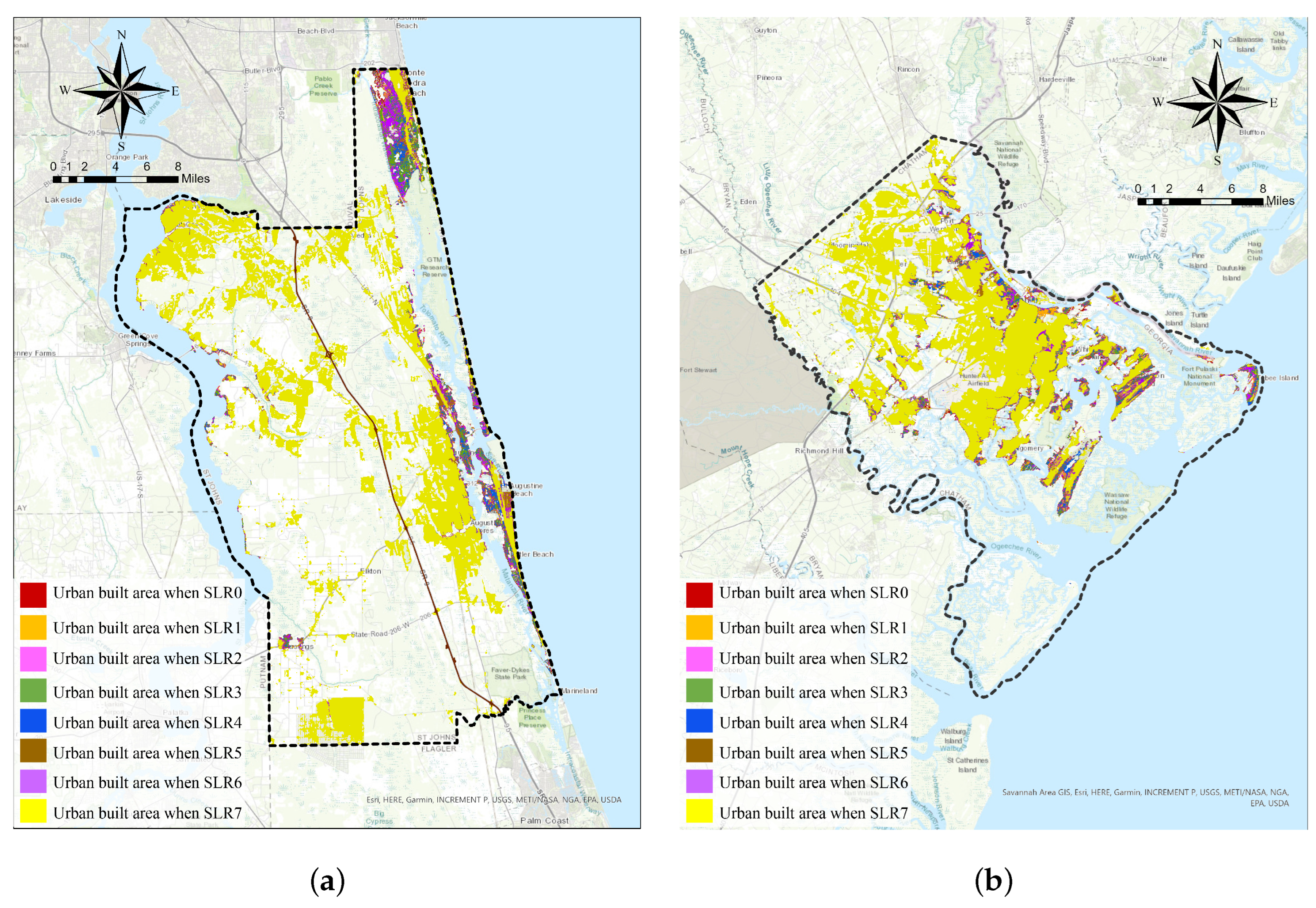
Figure A3.
Remaining urban built area maps when SLR transitions from 0 to 7 feet in St. Johns County.
Figure A3.
Remaining urban built area maps when SLR transitions from 0 to 7 feet in St. Johns County.
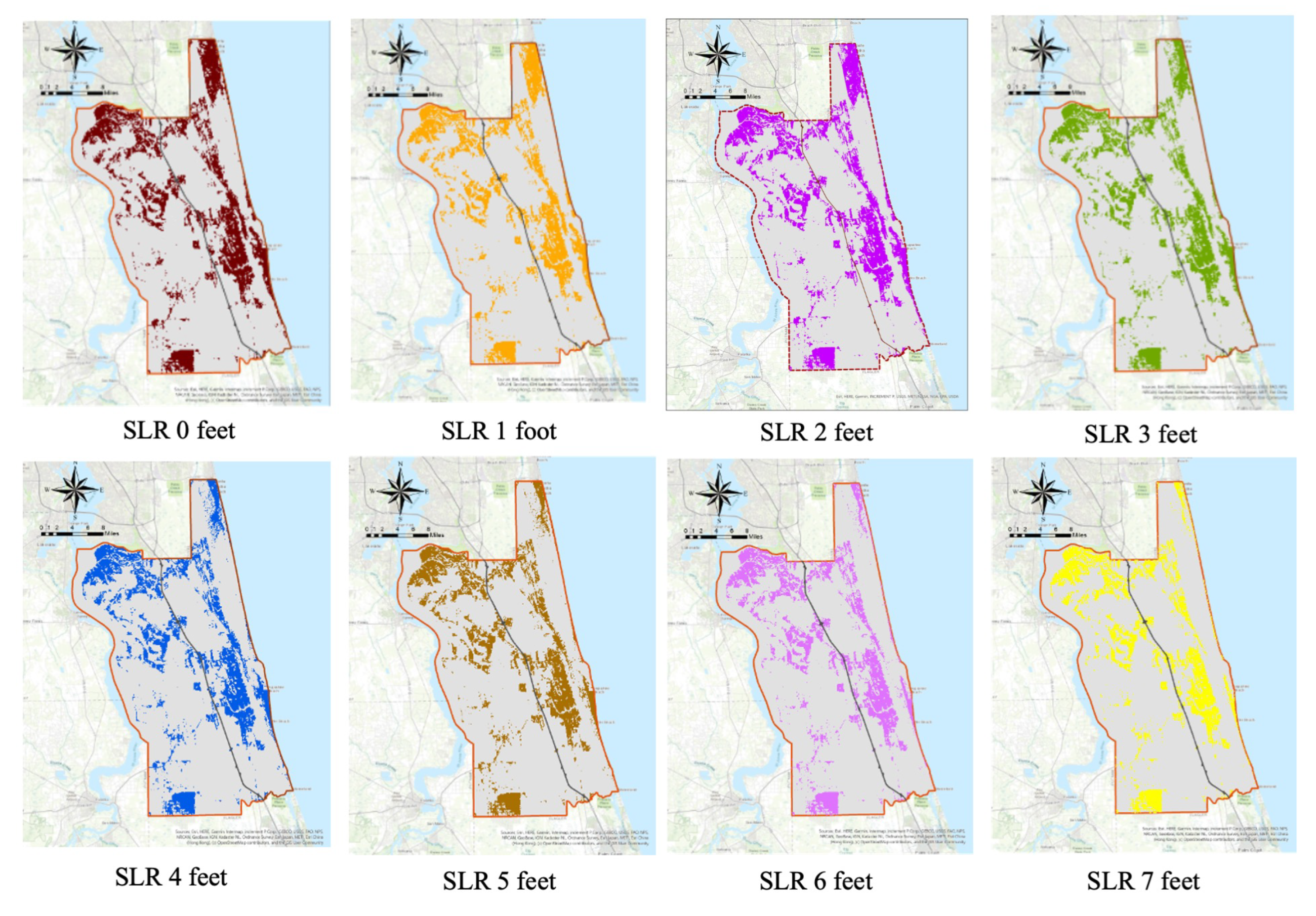
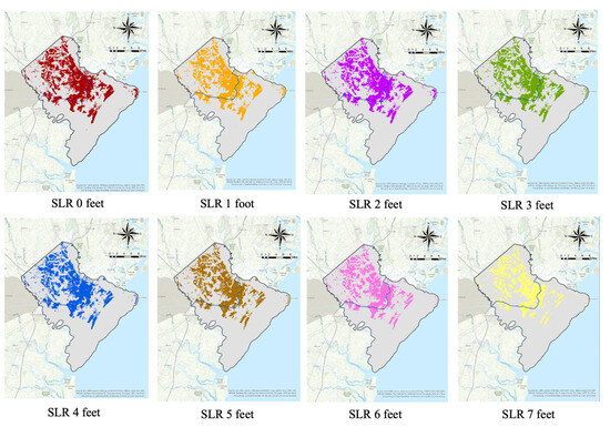
Figure A4.
Remaining urban built area maps when SLR transitions from 0 to 7 feet in Chatham County.
Figure A4.
Remaining urban built area maps when SLR transitions from 0 to 7 feet in Chatham County.
References
- Hauer, M.E.; Evans, J.M.; Mishra, D.R. Millions projected to be at risk from sea-level rise in the continental United States. Nat. Clim. Chang. 2016, 6, 691–695. [Google Scholar] [CrossRef]
- Bhattachan, A.; Jurjonas, M.D.; Moody, A.C.; Morris, P.R.; Sanchez, G.M.; Smart, L.S.; Taillie, P.J.; Emanuel, R.; Seekamp, E. Sea level rise impacts on rural coastal social-ecological systems and the implications for decision making. Environ. Sci. Policy 2018, 90, 122–134. [Google Scholar] [CrossRef]
- NOAA Sea Level Rise Viewer. Available online: https://coast.noaa.gov/slr/ (accessed on 9 January 2024).
- Surging Seas: Risk Zone Map. Available online: https://ss2.climatecentral.org/#12/40.7298/-74.0070?show=satellite&projections=0-K14_RCP85-SLR&level=5&unit=feet&pois=hide (accessed on 9 January 2024).
- Parris, A.S.; Bromirski, P.; Burkett, V.; Cayan, D.R.; Culver, M.E.; Hall, J.; Horton, R.M.; Knuuti, K.; Moss, R.H.; Obeysekera, J.; et al. Global Sea Level Rise Scenarios for the United States National Climate Assessment. 2012. Available online: https://repository.library.noaa.gov/view/noaa/11124 (accessed on 8 June 2024).
- Sweet, W.V.; Hamlington, B.D.; Kopp, R.E.; Weaver, C.P.; Barnard, P.L.; Bekaert, D.; Brooks, W.; Craghan, M.; Dusek, G.; Frederikse, T.; et al. Global and Regional Sea Level Rise Scenarios for the United States: Updated Mean Projections and Extreme Water Level Probabilities along US Coastlines; National Oceanic and Atmospheric Administration: Silver Spring, MD, USA, 2022; Available online: https://aambpublicoceanservice.blob.core.windows.net/oceanserviceprod/hazards/sealevelrise/noaa-nos-techrpt01-global-regional-SLR-scenarios-US.pdf (accessed on 8 June 2024).
- Morris, J.T.; Sundareshwar, P.; Nietch, C.T.; Kjerfve, B.; Cahoon, D.R. Responses of coastal wetlands to rising sea level. Ecology 2002, 83, 2869–2877. [Google Scholar] [CrossRef]
- Temmerman, S.; Govers, G.; Meire, P.; Wartel, S. Modelling long-term tidal marsh growth under changing tidal conditions and suspended sediment concentrations, Scheldt estuary, Belgium. Mar. Geol. 2003, 193, 151–169. [Google Scholar] [CrossRef]
- D’Alpaos, A.; Lanzoni, S.; Marani, M.; Rinaldo, A. Landscape evolution in tidal embayments: Modeling the interplay of erosion, sedimentation, and vegetation dynamics. J. Geophys. Res. Earth Surf. 2007, 112. [Google Scholar] [CrossRef]
- Kirwan, M.L.; Murray, A.B. A coupled geomorphic and ecological model of tidal marsh evolution. Proc. Natl. Acad. Sci. USA 2007, 104, 6118–6122. [Google Scholar] [CrossRef] [PubMed]
- Mudd, S.M.; Howell, S.M.; Morris, J.T. Impact of dynamic feedbacks between sedimentation, sea-level rise, and biomass production on near-surface marsh stratigraphy and carbon accumulation. Estuar. Coast. Shelf Sci. 2009, 82, 377–389. [Google Scholar] [CrossRef]
- Kirwan, M.L.; Guntenspergen, G.R.; d’Alpaos, A.; Morris, J.T.; Mudd, S.M.; Temmerman, S. Limits on the adaptability of coastal marshes to rising sea level. Geophys. Res. Lett. 2010, 37. [Google Scholar] [CrossRef]
- McGarigal, K. FRAGSTATS: Spatial Pattern Analysis Program for Quantifying Landscape Structure; US Department of Agriculture, Forest Service, Pacific Northwest Research Station: Washington, DC, USA, 1995; Volume 351. [Google Scholar]
- Li, X.; Lu, L.; Cheng, G.; Xiao, H. Quantifying landscape structure of the Heihe River Basin, north-west China using FRAGSTATS. J. Arid. Environ. 2001, 48, 521–535. [Google Scholar] [CrossRef]
- Olsen, L.M.; Dale, V.H.; Foster, T. Landscape patterns as indicators of ecological change at Fort Benning, Georgia, USA. Landsc. Urban Plan. 2007, 79, 137–149. [Google Scholar] [CrossRef]
- Kamusoko, C.; Aniya, M. Land use/cover change and landscape fragmentation analysis in the Bindura District, Zimbabwe. Land Degrad. Dev. 2007, 18, 221–233. [Google Scholar] [CrossRef]
- Singh, S.K.; Srivastava, P.K.; Szabó, S.; Petropoulos, G.P.; Gupta, M.; Islam, T. Landscape transform and spatial metrics for mapping spatiotemporal land cover dynamics using Earth Observation data-sets. Geocarto Int. 2017, 32, 113–127. [Google Scholar] [CrossRef]
- Smiraglia, D.; Ceccarelli, T.; Bajocco, S.; Perini, L.; Salvati, L. Unraveling landscape complexity: Land use/land cover changes and landscape pattern dynamics (1954–2008) in contrasting peri-urban and agro-forest regions of northern Italy. Environ. Manag. 2015, 56, 916–932. [Google Scholar] [CrossRef] [PubMed]
- Zhang, Z.; Meerow, S.; Newell, J.P.; Lindquist, M. Enhancing landscape connectivity through multifunctional green infrastructure corridor modeling and design. Urban For. Urban Green. 2019, 38, 305–317. [Google Scholar] [CrossRef]
- Singh, S.K.; Pandey, A.C.; Singh, D. Land use fragmentation analysis using remote sensing and Fragstats. In Remote Sensing Applications in Environmental Research; Springer: Berlin/Heidelberg, Germany, 2014; pp. 151–176. [Google Scholar]
- Uuemaa, E.; Antrop, M.; Roosaare, J.; Marja, R.; Mander, Ü. Landscape metrics and indices: An overview of their use in landscape research. Living Rev. Landsc. Res. 2009, 3, 1–28. [Google Scholar] [CrossRef]
- Wurm, M. Oliveira, Vítor (2016): Urban Morphology. An Introduction to the Study of the Physical Form of Cities; The Urban Book Series; XXIII. 192 Seiten, 46 s/w-Illustrationen, 19 Farbige Illustrationen; Springer International Publishing: Cham, Switzerland, 2017. [Google Scholar]
- Hurlimann, A.; Barnett, J.; Fincher, R.; Osbaldiston, N.; Mortreux, C.; Graham, S. Urban planning and sustainable adaptation to sea-level rise. Landsc. Urban Plan. 2014, 126, 84–93. [Google Scholar] [CrossRef]
- Borchert, S.M.; Osland, M.J.; Enwright, N.M.; Griffith, K.T. Coastal wetland adaptation to sea level rise: Quantifying potential for landward migration and coastal squeeze. J. Appl. Ecol. 2018, 55, 2876–2887. [Google Scholar] [CrossRef]
- Christie, D.R. Florida’s ocean future: Toward a state ocean policy. J. Land Use Environ. Law 1989, 5, 447. [Google Scholar]
- Dovey, K.; Pafka, E.; Ristic, M. Mapping Urbanities: Morphologies, Flows, Possibilities; Routledge: London, UK, 2017. [Google Scholar]
- Pörtner, H.O.; Roberts, D.; Tignor, M.; Poloczanska, E.; Mintenbeck, K.; Alegría, A.; Craig, M.; Langsdorf, S.; Löschke, S.; Möller, V.; et al. (Eds.) Climate Change 2022: Impacts, Adaptation and Vulnerability. Contribution of Working Group II to the Sixth Assessment Report of the Intergovernmental Panel on Climate Change; Cambridge University Press: Cambridge, UK; New York, NY, USA, 2022; p. 3056. [Google Scholar] [CrossRef]
- The NASA Sea Level Projection Tool. Available online: https://sealevel.nasa.gov/ipcc-ar6-sea-level-projection-tool (accessed on 31 May 2024).
- Hinkel, J.; Jaeger, C.; Nicholls, R.J.; Lowe, J.; Renn, O.; Peijun, S. Sea-level rise scenarios and coastal risk management. Nat. Clim. Chang. 2015, 5, 188–190. [Google Scholar] [CrossRef]
- Kupfer, J.A. Landscape ecology and biogeography: Rethinking landscape metrics in a post-FRAGSTATS landscape. Prog. Phys. Geogr. 2012, 36, 400–420. [Google Scholar] [CrossRef]
- Guan, Y.; Lu, H.; He, L.; Adhikari, H.; Pellikka, P.; Maeda, E.; Heiskanen, J. Intensification of the dispersion of the global climatic landscape and its potential as a new climate change indicator. Environ. Res. Lett. 2020, 15, 114032. [Google Scholar] [CrossRef]
- Jaafari, S.; Shabani, A.A.; Moeinaddini, M.; Danehkar, A.; Sakieh, Y. Applying landscape metrics and structural equation modeling to predict the effect of urban green space on air pollution and respiratory mortality in Tehran. Environ. Monit. Assess. 2020, 192, 412. [Google Scholar] [CrossRef] [PubMed]
- Das, S.; Angadi, D.P. Assessment of urban sprawl using landscape metrics and Shannon’s entropy model approach in town level of Barrackpore sub-divisional region, India. Model. Earth Syst. Environ. 2021, 7, 1071–1095. [Google Scholar] [CrossRef]
- Bosch, M.; Jaligot, R.; Chenal, J. Spatiotemporal patterns of urbanization in three Swiss urban agglomerations: Insights from landscape metrics, growth modes and fractal analysis. Landsc. Ecol. 2020, 35, 879–891. [Google Scholar] [CrossRef]
- Bianchin, S.; Richert, E.; Heilmeier, H.; Merta, M.; Seidler, C. Landscape metrics as a tool for evaluating scenarios for flood prevention and nature conservation. Landsc. Online 2011, 25, 1–11. [Google Scholar] [CrossRef]
- Epting, S.M.; Hosen, J.D.; Alexander, L.C.; Lang, M.W.; Armstrong, A.W.; Palmer, M.A. Landscape metrics as predictors of hydrologic connectivity between Coastal Plain forested wetlands and streams. Hydrol. Process. 2018, 32, 516–532. [Google Scholar] [CrossRef] [PubMed]
- Parker, S.R. The Second Century of Settlement in Spanish St. Augustine, 1670–1763; University of Florida: Gainesville, FL, USA, 1999. [Google Scholar]
- Gannon, M. The New History of Florida; University Press of Florida: Tallahassee, FL, USA, 1996; Volume 15. [Google Scholar]
- Wilson, T.D. The Oglethorpe Plan: Enlightenment Design in Savannah and Beyond; University of Virginia Press: Charlottesville, VA, USA, 2015. [Google Scholar]
- Bolster, P. Saving the Georgia Coast: A Political History of the Coastal Marshlands Protection Act; University of Georgia Press: Athens, GA, USA, 2020; Volume 36. [Google Scholar]
- Firehock, K. Evaluating and Conserving Green Infrastructure across the Landscape: A Practitioner’s Guide; The Green Infrastructure Center Inc.: Charlottesville, VA, USA, 2013; Available online: https://gicinc.org/wp-content/uploads/Evaluating-and-Conserving-GI-A-practitioners-guide-VA-Edition_2012_web.pdf (accessed on 8 June 2024).
- Forman, R.T.; Godron, M. Patches and structural components for a landscape ecology. BioScience 1981, 31, 733–740. [Google Scholar]
- Wijaya, A.; Susetyo, C.; Diny, A.Q.; Nabila, D.H.; Pamungkas, R.P.; Hadikunnuha, M.; Pratomoatmojo, N.A. Spatial Pattern Dynamics Analysis in Coastal Area Using Spatial Metric in Pekalongan, Indonesia. Preprints 2017. [Google Scholar] [CrossRef]
- Mangipanea, L.S.; Belant, J.L.; Hiller, T.L.; Colvin, M.E.; Gustine, D.D.; Mangipane, B.A.; Hilderbrand, G.V. Influences of landscape heterogeneity on home-range sizes of brown bears. Mamm. Biol. 2018, 88, 1–7. [Google Scholar] [CrossRef]
- Pham, H.M.; Yamaguchi, Y. Urban growth and change analysis using remote sensing and spatial metrics from 1975 to 2003 for Hanoi, Vietnam. Int. J. Remote Sens. 2011, 32, 1901–1915. [Google Scholar] [CrossRef]
- Firehock, K.; Walker, R.A. Strategic Green Infrastructure Planning: A Multi-Scale Approach; Island Press: Lahaina, HI, USA, 2015. [Google Scholar]
- Hannibal, W.; Cunha, N.L.d.; Figueiredo, V.V.; Rossi, R.F.; Cáceres, N.C.; Ferreira, V.L. Multi-scale approach to disentangle the small mammal composition in a fragmented landscape in central Brazil. J. Mammal. 2018, 99, 1455–1464. [Google Scholar] [CrossRef]
- Ji, W.; Ma, J.; Twibell, R.W.; Underhill, K. Characterizing urban sprawl using multi-stage remote sensing images and landscape metrics. Comput. Environ. Urban Syst. 2006, 30, 861–879. [Google Scholar] [CrossRef]
- Kumar, M.; Denis, D.M.; Singh, S.K.; Szabó, S.; Suryavanshi, S. Landscape metrics for assessment of land cover change and fragmentation of a heterogeneous watershed. Remote Sens. Appl. Soc. Environ. 2018, 10, 224–233. [Google Scholar] [CrossRef]
- Magidi, J.; Ahmed, F. Assessing urban sprawl using remote sensing and landscape metrics: A case study of City of Tshwane, South Africa (1984–2015). Egypt. J. Remote Sens. Space Sci. 2019, 22, 335–346. [Google Scholar] [CrossRef]
- Lausch, A.; Herzog, F. Applicability of landscape metrics for the monitoring of landscape change: Issues of scale, resolution and interpretability. Ecol. Indic. 2002, 2, 3–15. [Google Scholar] [CrossRef]
- Sudhira, H.; Ramachandra, T. Characterising urban sprawl from remote sensing data and using landscape metrics. In Proceedings of the 10th International Conference on Computers in Urban Planning and Urban Management, Iguassu Falls, Brazil, 11–13 July 2007; Citeseer: University Park, PA, USA, 2007; pp. 11–13. [Google Scholar]
- Zubair, O.A. Investigating urban growth and the dynamics of urban land cover change using remote sensing data and landscape metrics. Pap. Appl. Geogr. 2021, 7, 67–81. [Google Scholar] [CrossRef]
- Herzog, F.; Lausch, A.; MÜller, E.; Thulke, H.h.; Steinhardt, U.; Lehmann, S. Landscape metrics for assessment of landscape destruction and rehabilitation. Environ. Manag. 2001, 27, 91–107. [Google Scholar] [CrossRef]


Disclaimer/Publisher’s Note: The statements, opinions and data contained in all publications are solely those of the individual author(s) and contributor(s) and not of MDPI and/or the editor(s). MDPI and/or the editor(s) disclaim responsibility for any injury to people or property resulting from any ideas, methods, instructions or products referred to in the content. |
© 2024 by the authors. Licensee MDPI, Basel, Switzerland. This article is an open access article distributed under the terms and conditions of the Creative Commons Attribution (CC BY) license (https://creativecommons.org/licenses/by/4.0/).