
An Identification Method of Corner Reflector Array Based on Mismatched Filter through Changing the Frequency Modulation Slope

Abstract
:1. Introduction
- Stable performance. The recognition process aims to utilise the structural dissimilarities between the two targets in order to achieve recognition, rather than relying on some intuitive features, such as length or the number of scattering points, which is applicable to complex environments. Compared to the methods applied in HRRP, the proposed method is not limited to some environmental factors, such as the number of corner reflectors or the observation angle. In contrast to the aforementioned frequency domain features, this approach is not limited to scenarios where there are differences in the speed of targets.
- Strong applicability. The primary objective of this method is to enhance the performance of the LFM radar, which is a common waveform in radar systems. Nevertheless, the efficacy of polarization decomposition is contingent upon the availability of a fully polarimetric radar and a signal possessing a high degree of polarization isolation, both of which are essential for the accurate measurement to guarantee its performance. The methods employed in the frequency domain similarly necessitate the capacity for coherent integration.
2. Mismatched Filter by Changing Frequency Modulation Slope
2.1. Signal Model
2.2. Mismatched Filter by Modifying Frequency Modulation Slope
2.3. Analysis on Echoes Simulated from Simple Scattering Points
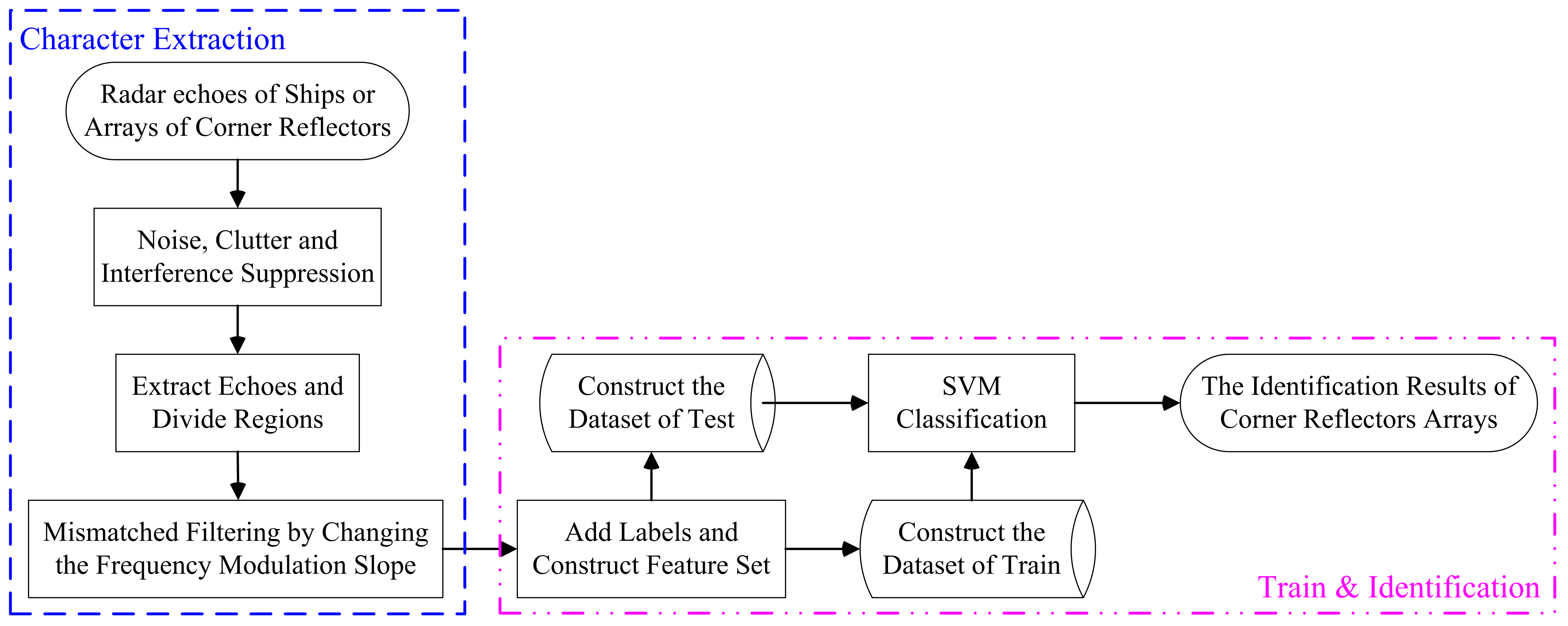
3. Character Extraction and Identification
3.1. Target Echo Acquisition
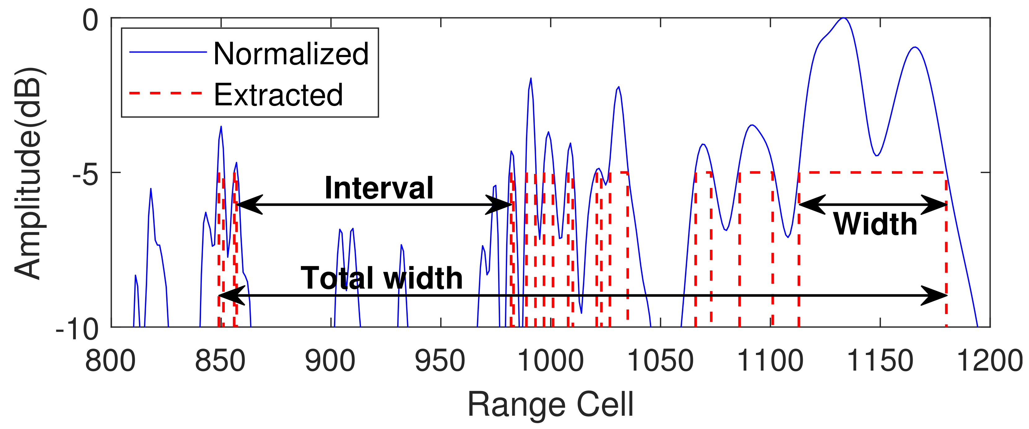
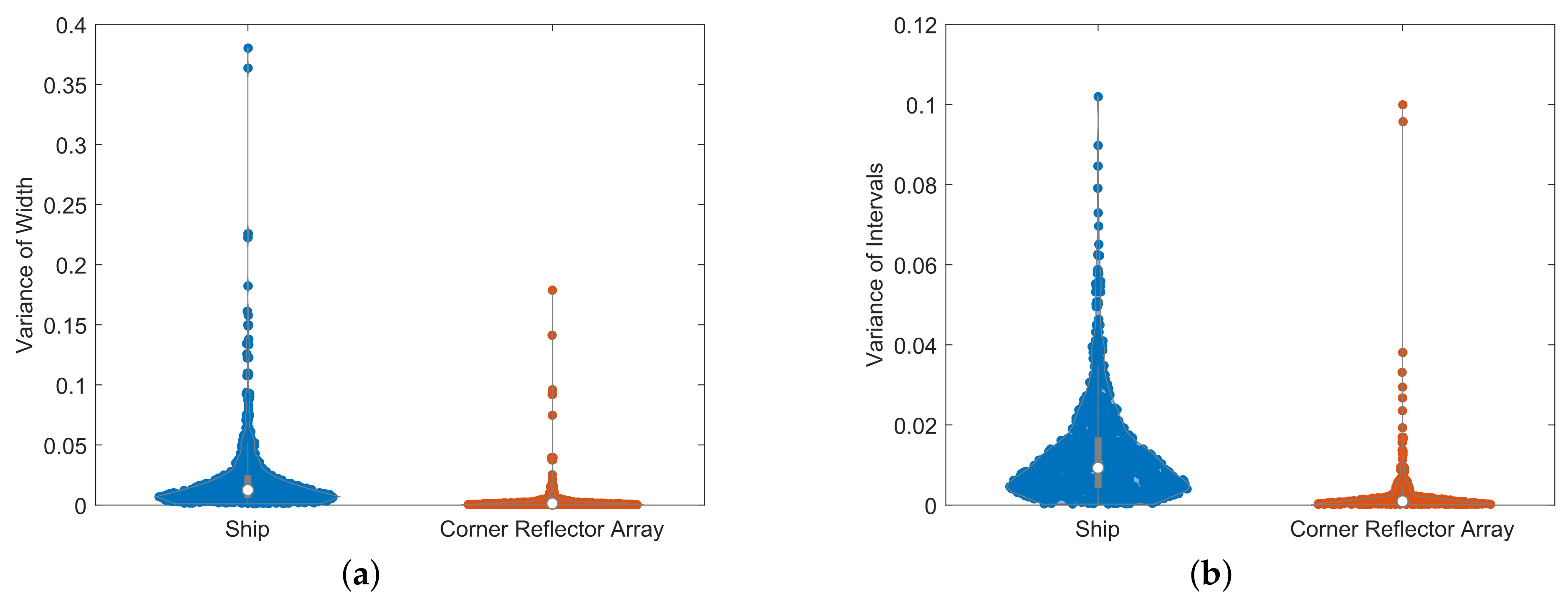
3.2. Character Extraction
3.3. Identification Method Based on SVM
4. Simulation Experiment Analysis
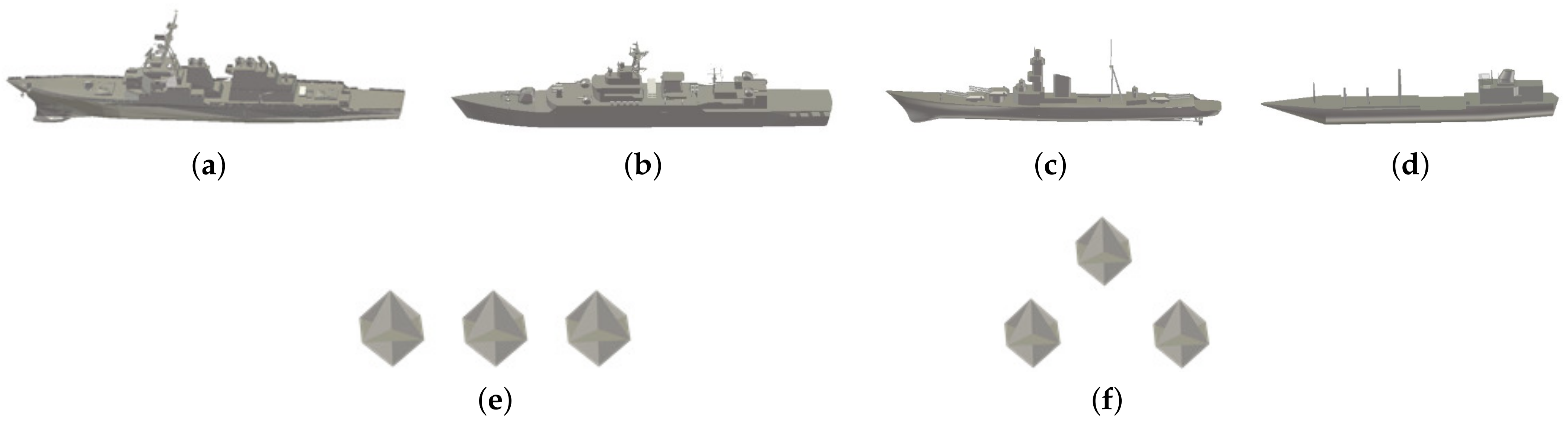
4.1. Data Acquisition
4.2. Identification Based on a Single Modification Factor
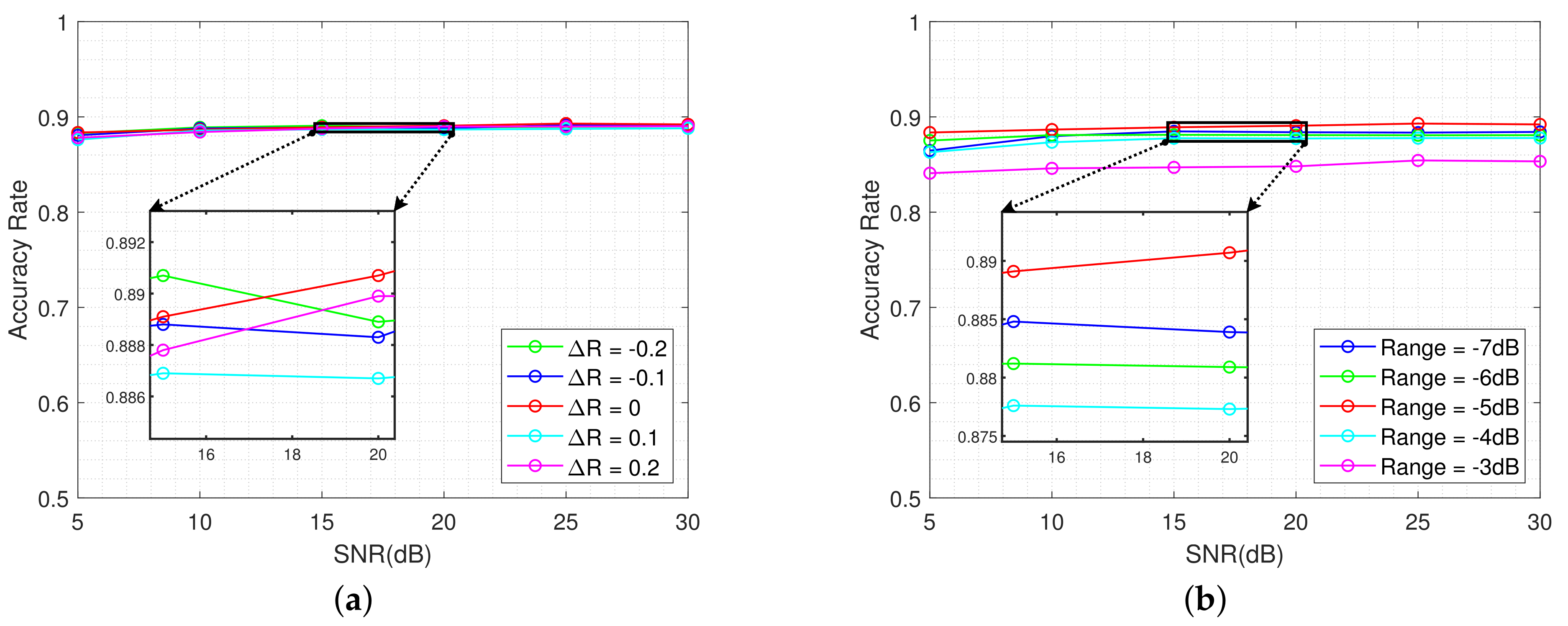
4.3. Identification Based on a Range of Modulation Factors
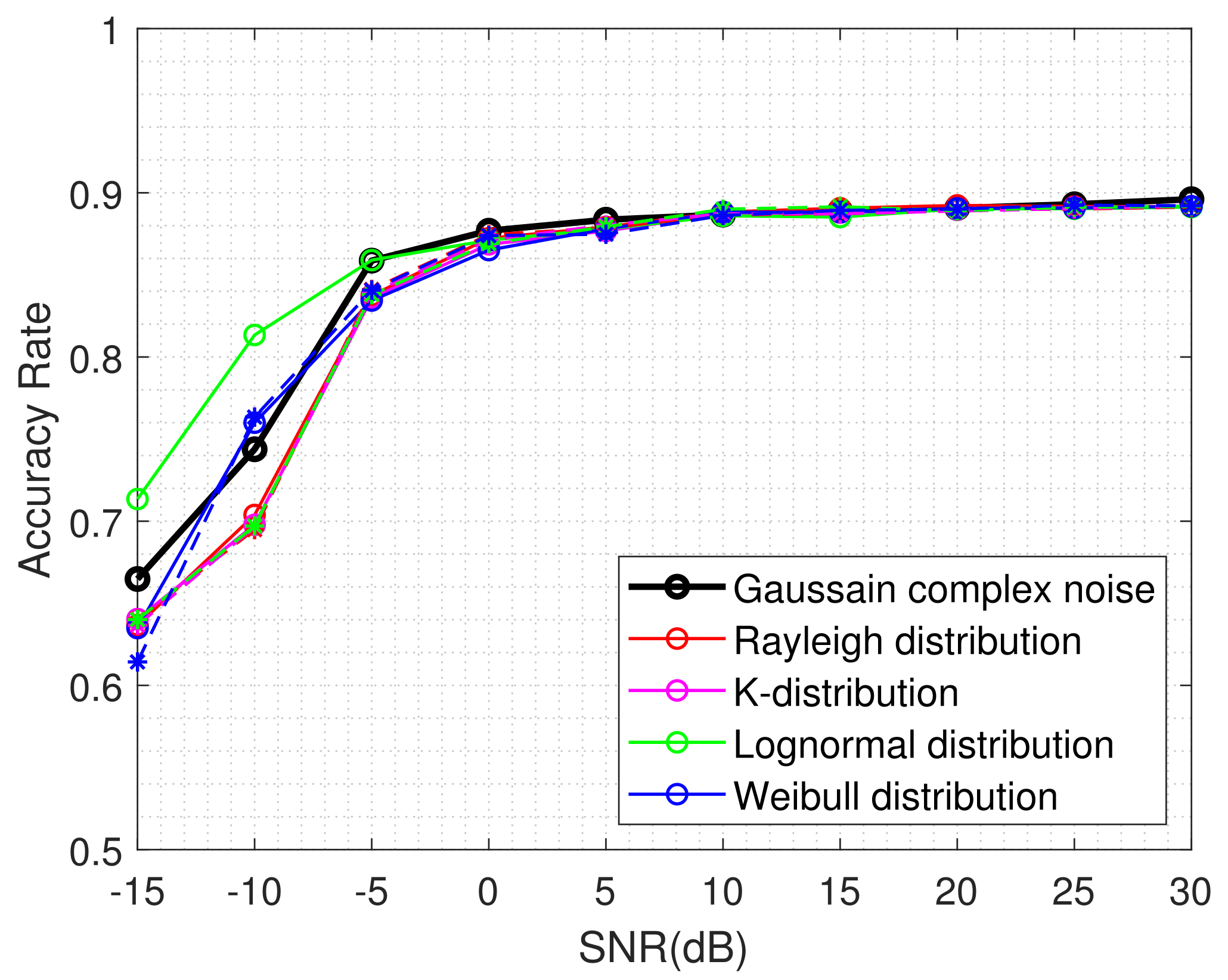
4.4. Stability Tests under Different Conditions
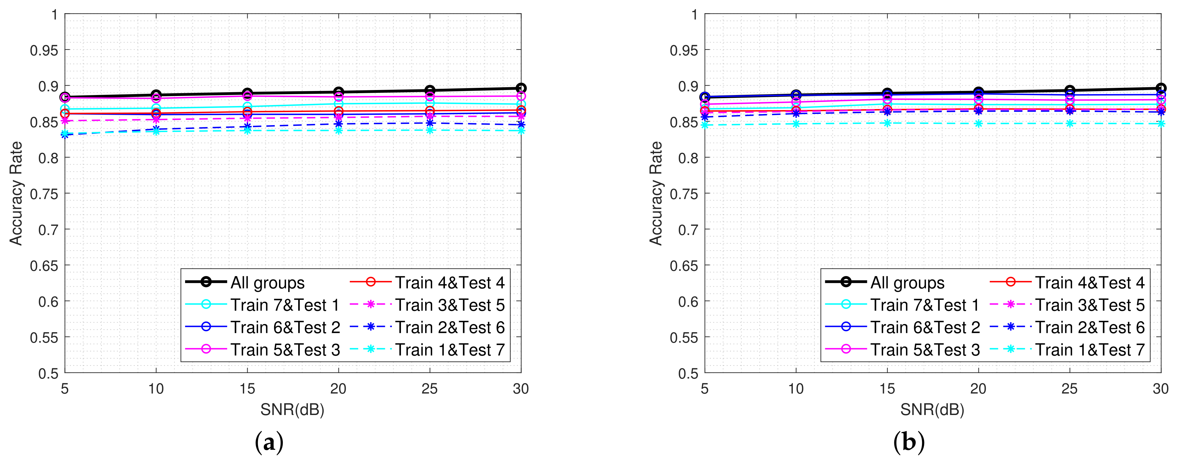
4.5. Stability Tests under Different Quantities of Corner Reflectors
5. Conclusions
Author Contributions
Funding
Data Availability Statement
Conflicts of Interest
References
- Li, H.; Chen, S. Electromagnetic scattering characteristics and radar identification of sea corner reflectors: Advances and prospects. J. Radars 2023, 12, 738–761. [Google Scholar]
- Wu, L.; Xu, J.; Hu, S.; Liu, Z. High-frequency backscattering properties of quasi-omnidirectional corner reflector: The great-icosahedral-like reflector. AIP Adv. 2022, 12, 105225. [Google Scholar] [CrossRef]
- Zhang, Z.; Zhang, J.; Qu, S.; Du, H. Research on radar corner reflector: Advances and perspectives. Aerodyn. Missile J. 2014, 4, 64–70. [Google Scholar]
- Luo, Y.; Guo, L.X.; Zuo, Y.; Liu, W. Time-domain scattering characteristics and jamming effectiveness in corner reflectors. IEEE Access 2021, 9, 15696–15707. [Google Scholar] [CrossRef]
- Jiang, T.; Luo, J.; Yu, Z. Research on corner reflector array fitting method for ship scattering characteristics. In Proceedings of the 2023 IEEE 2nd International Conference on Electrical Engineering, Big Data and Algorithms (EEBDA), Changchun, China, 24–26 February 2023. [Google Scholar]
- Zhang, J.; Hu, S.; Wu, L.; Fan, X.; Yang, Q. Air-floating corner reflectors dilution jamming placement position. In Proceedings of the 2019 IEEE 8th Data Driven Control and Learning Systems Conference (DDCLS), Dali, China, 24–27 May 2019. [Google Scholar]
- Wu, G.; Wang, L.; Pang, C.; Li, Y.; Wang, X. Radar polarization modulation countermeasures for combined corner reflector: Anti diluted jamming. Acta Electron. Sin. 2022, 50, 2969–2983. [Google Scholar]
- Han, J.; Yang, Y.; Lian, J.; Wu, G.; Wang, X. Identification method of corner reflector based on polarization and HRRP feature fusion for radar seeker. J. Syst. Eng. Electron. 2023; in press. [Google Scholar]
- Tang, G.; Li, H.; Gan, R.; Yuan, R. Analysis of corner reflector under naval battlefield. Electron. Inf. Warf. Technol. 2015, 30, 39–45+84. [Google Scholar]
- Wang, L.; Jiang, N.; Sun, Y. The mechanism analyzing and use of corner reflector against anti-ship missiles. In Proceedings of the 2017 5th International Conference on Mechatronics, Materials, Chemistry and Computer Engineering (ICMMCCE 2017), Chongqing, China, 24–25 July 2017. [Google Scholar]
- Zhou, X.; Zhu, J.; Yu, W.; Cui, T. Time-domain shooting and bouncing rays method based on beam tracing technique. IEEE Trans. Antennas Propag. 2015, 63, 4037–4048. [Google Scholar] [CrossRef]
- Yuan, H.; Fu, X.; Zhao, C.; Xie, M.; Gao, X. Ship and Corner Reflector Identification Based on Extreme Learning Machine. In Proceedings of the 2019 IEEE International Conference on Signal, Information and Data Processing (ICSIDP), Chongqing, China, 11–13 December 2019. [Google Scholar]
- Zeng, Z.; Sun, J.; Han, Z.; Hong, W. Radar HRRP target recognition method based on multi-input convolutional gated recurrent unit with cascaded feature fusion. IEEE Geosci. Remote Sens. Lett. 2022, 19, 4026005. [Google Scholar] [CrossRef]
- Lv, F. Dynamic Echo Simulation and Characteristic Analysis of Sea Surface Targets. Master Dissertation, Xidian University, Xi’an, China, 2019. [Google Scholar]
- Cui, K.; Wang, W.; Chen, X.; Yuan, N. A kind of method of anti-corner reflector interference for millimeter wave high resolution radar system. In Proceedings of the 2016 Progress in Electromagnetic Research Symposium (PIERS), Shanghai, China, 8–11 August 2016. [Google Scholar]
- Shi, F.; Li, Z.; Zhang, M.; Li, J. Analysis and Simulation of the Micro-Doppler Signature of a Ship with a Rotating Shipborne Radar at Different Observation Angles. IEEE Geosci. Remote Sens. Lett. 2022, 19, 1504405. [Google Scholar] [CrossRef]
- Hanif, A.; Muaz, M.; Hasan, A.; Adeel, M. Micro-Doppler Based Target Recognition With Radars: A Review. IEEE Sens. J. 2022, 22, 2948–2961. [Google Scholar] [CrossRef]
- Fang, M.; Zhu, Y.; Huang, M.; Fu, Q. Sea surface target polarization feature extraction based on modified odd-time and even-time scattering models. In Proceedings of the 2013 2nd International Conference on Measurement, Information and Control, Harbin, China, 16–18 August 2013. [Google Scholar]
- Liang, Z.; Yu, Y.; Zhang, B. Anti-corner reflector array method based on pauli polarization decomposition and BP neural network. In Proceedings of the 2021 IEEE 2nd International Conference on Pattern Recognition and Machine Learning (PRML), Chengdu, China, 16–18 July 2021. [Google Scholar]
- Cloude, S.R.; Pottier, E. A review of target decomposition theorems in radar polarimetry. IEEE Trans. Geosci. Remote Sens. 1996, 34, 498–518. [Google Scholar] [CrossRef]
- Krogager, E. New decomposition of the radar target scattering matrix. Electron. Lett. 1990, 26, 1525–1532. [Google Scholar] [CrossRef]
- Chen, S.; Li, Y.; Wang, X.; Xiao, S.; Sato, M. Modeling and Interpretation of Scattering Mechanisms in Polarimetric Synthetic Aperture Radar: Advances and perspectives. IEEE Signal Proc. Mag. 2014, 31, 79–89. [Google Scholar] [CrossRef]
- Li, H.; Li, M.; Cui, X.; Chen, S. Man-made target structure recognition with polarimetric correlation pattern and roll-invariant feature coding. IEEE Geosci. Remote Sens. Lett. 2022, 19, 8024105. [Google Scholar] [CrossRef]
- Liang, Z.; Wang, Y.; Zhao, X.; Xie, M.; Fu, X. Identification of ship and corner reflector in sea clutter environment. In Proceedings of the 2020 15th IEEE International Conference on Signal Processing (ICSP), Beijing, China, 6–9 December 2020. [Google Scholar]
- Chen, S.; Wu, G.; Dai, D.; Wang, X.; Xiao, S. Roll-Invariant Features in Radar Polarimetry: A Survey. In Proceedings of the IGARSS 2019–2019 IEEE International Geoscience and Remote Sensing Symposium, Yokohama, Japan, 28 July–2 August 2019. [Google Scholar]
- He, Y.; Yang, H.; He, H.; Yin, J.; Yang, J. A Ship Discrimination Method Based on High-Frequency Electromagnetic Theory. Remote Sens. 2022, 14, 3893. [Google Scholar] [CrossRef]
- Yu, K.; Zhu, S.; Lan, L.; Zhu, J.; Li, X. Mainbeam Deceptive Jammer Suppression With Joint Element-Pulse Phase Coding. IEEE Trans. Veh. Technol. 2024, 73, 2332–2344. [Google Scholar] [CrossRef]
- Wang, F.; Li, N.; Pang, C.; Li, Y.; Wang, X. Algorithm for Designing PCFM Waveforms for Simultaneously Polarimetric Radars. IEEE Trans. Geosci. Remote Sens. 2024, 62, 5100716. [Google Scholar] [CrossRef]
- Jin, L.; Wang, J.; Zhong, Y.; Wang, D. Optimal Mismatched Filter Design by Combining Convex Optimization with Circular Algorithm. IEEE Access 2022, 10, 56763–56772. [Google Scholar] [CrossRef]
- Mattingly, R.G.; Martone, A.F.; Metcalf, J.G. Techniques for Mitigating the Impact of Intra-CPI Waveform Agility. IEEE Trans. Radar Syst. 2024, 2, 24–40. [Google Scholar] [CrossRef]
- Liu, G.; Gao, W.; Liu, W.; Xu, J.; Li, R.; Bai, W. LFM-Chirp-Square pulse-compression thermography for debonding defects detection in honeycomb sandwich composites based on THD-processing technique. Nondestruct. Test. Eval. 2024, 39, 832–845. [Google Scholar] [CrossRef]
- Dai, H.; Zhao, Y.; Su, H.; Wang, Z.; Bao, Q.; Pan, J. Research on an intra-pulse orthogonal waveform and methods resisting interrupted-sampling repeater jamming within the same frequency band. Remote Sens. 2023, 15, 3673. [Google Scholar] [CrossRef]
- Kouyoumjian, R.G.; Pathak, P.H. A uniform geometrical theory of diffraction for an edge in a perfectly conducting surface. IEEE Trans. Signal Process. 1974, 62, 1448–1461. [Google Scholar] [CrossRef]
- Ghasemi, M.; Sheikhi, A. Joint Scattering Center Enumeration and Parameter Estimation in GTD Model. IEEE Trans. Antenn. Propag. 2020, 68, 4786–4798. [Google Scholar] [CrossRef]
- Hu, P.; Xu, S.; Zou, J.; Chen, Z. Parameter estimation of GTD model using iterative adaptive approach. In Proceedings of the 2017 IEEE SENSORS, Glasgow, UK, 29 October–1 November 2017. [Google Scholar]
- Chen, S.; Pan, M. Analytical Model and Real-Time Calculation of Target Echo Signals on Wideband LFM Radar. IEEE Sens. J. 2021, 21, 10726–10734. [Google Scholar] [CrossRef]
- Li, S.; Wang, X.; Fu, Z.; Zhang, J. Extraction of scattering center parameter and RCS reconstruction based on the improved TLS-ESPRIT algorithm of Hankel matrix. J. Syst. Eng. Electron. 2021, 43, 62–73. [Google Scholar]
- Zhou, Z. Machine Learning, 1st ed.; Tsinghua University Press: Beijing, China, 2016; pp. 121–139. [Google Scholar]
- Lu, Z.; Wang, Z.; Dan, B. Ship target identification method based on the characteristic of target polarimetric HRRP of radars. In Proceedings of the 2022 Global Reliability and Prognostics and Health Management (PHM-Yantai), Yantai, China, 13–16 October 2022. [Google Scholar]
- Zhu, Z.; Tang, G.; Cheng, Z.; Huang, P. Discrimination method of ship and corner reflector based on polarization decomposition. Shipboard Electron. Countermeas. 2010, 33, 15–21. [Google Scholar]
- Wang, M.; Xie, M.; Su, Q.; Fu, X. Identification of ship and corner reflector based on invariant features of the polarization. In Proceedings of the 2019 IEEE 4th International Conference on Signal and Image Processing (ICSIP), Wuxi, China, 19–21 July 2019. [Google Scholar]
- Shi, Y.; Shui, P. Target detection in high-resolution sea clutter via block-adaptive clutter suppression. IET Radar Sonar Navigat. 2011, 5, 48–57. [Google Scholar] [CrossRef]
- Chen, M.; Li, L.; Geng, Z.; Xie, X. Single-channel Blind Source Separation Algorithm Based on Water Area Noise Characteristics. In Proceedings of the 2022 IEEE International Conference on Mechatronics and Automation (ICMA), Guilin, China, 7–10 August 2022. [Google Scholar]
- Lv, M.; Zhou, C. Study on Sea Clutter Suppression Methods Based on a Realistic Radar Dataset. Remote Sens. 2019, 11, 2721. [Google Scholar] [CrossRef]
- Zhu, J.; Tang, J. K-distribution Clutter Simulation Methods Based on Improved ZMNL and SIRP. J. Radars 2014, 3, 533–540. [Google Scholar] [CrossRef]
- Gao, Z.; Zhang, A. Simulation Analysis of Typical Amplitude Distribution Model of Sea Clutter. Ship Electron. Eng. 2018, 38, 76–79. [Google Scholar]
- The McMaster IPIX Radar Sea Clutter Database. Available online: http://soma.mcmaster.ca/ipix/ (accessed on 29 May 2024).


| Scenario | Distribution of Position | Types of Scattering Points |
|---|---|---|
| 1 | Uniform | Consistent |
| 2 | Uniform | Inconsistent |
| 3 | Cluster 1 | Consistent |
| 4 | Cluster | Inconsistent |
| Type | Length (m) | Width (m) | Height (m) |
|---|---|---|---|
| Ship 1 | 169.39 | 22.90 | 56.25 |
| Ship 2 | 145.35 | 17.74 | 34.27 |
| Ship 3 | 107.74 | 11.39 | 29.14 |
| Ship 4 | 130.80 | 10.12 | 23.32 |
| Type of Ship | Type of Array 1 | Number of Arrays |
|---|---|---|
| Ship 1 | Array 1 | 2 |
| Array 2 | 2 | |
| Ship 2 | Array 1 | 1 |
| Array 2 | 2 | |
| Ship 3 | Array 1 | 1 |
| Array 2 | 2 | |
| Ship 4 | Array 1 | 2 |
| Array 2 | 2 |
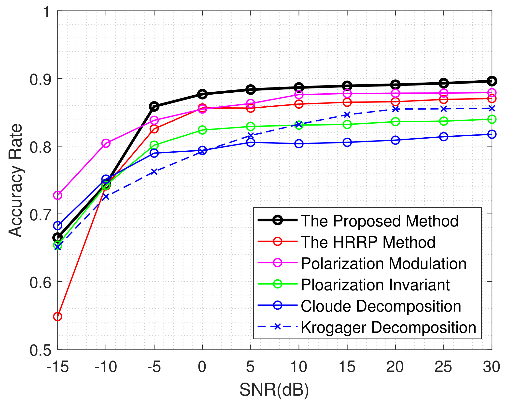
| Methods | −15 | −10 | −5 | 0 | 5 | 10 | 15 | 20 | 25 | 30 |
|---|---|---|---|---|---|---|---|---|---|---|
| The Proposed Method | 0.665 | 0.744 | 0.858 | 0.877 | 0.884 | 0.887 | 0.889 | 0.891 | 0.893 | 0.896 |
| HRRP Method in [8] | 0.548 | 0.741 | 0.827 | 0.857 | 0.856 | 0.862 | 0.864 | 0.866 | 0.869 | 0.871 |
| Polarization Modulation [7] | 0.727 | 0.804 | 0.838 | 0.855 | 0.863 | 0.876 | 0.878 | 0.878 | 0.878 | 0.879 |
| Polarization Invariant [41] | 0.654 | 0.742 | 0.801 | 0.824 | 0.829 | 0.831 | 0.832 | 0.836 | 0.837 | 0.840 |
| Cloude Decomposition [39] | 0.683 | 0.751 | 0.790 | 0.794 | 0.806 | 0.804 | 0.806 | 0.809 | 0.814 | 0.818 |
| Krogager decomposition [40] | 0.651 | 0.725 | 0.762 | 0.792 | 0.816 | 0.832 | 0.847 | 0.855 | 0.855 | 0.856 |
Disclaimer/Publisher’s Note: The statements, opinions and data contained in all publications are solely those of the individual author(s) and contributor(s) and not of MDPI and/or the editor(s). MDPI and/or the editor(s) disclaim responsibility for any injury to people or property resulting from any ideas, methods, instructions or products referred to in the content. |
© 2024 by the authors. Licensee MDPI, Basel, Switzerland. This article is an open access article distributed under the terms and conditions of the Creative Commons Attribution (CC BY) license (https://creativecommons.org/licenses/by/4.0/).
Share and Cite
Xia, L.; Wang, F.; Pang, C.; Li, N.; Peng, R.; Song, Z.; Li, Y. An Identification Method of Corner Reflector Array Based on Mismatched Filter through Changing the Frequency Modulation Slope. Remote Sens. 2024, 16, 2114. https://doi.org/10.3390/rs16122114
Xia L, Wang F, Pang C, Li N, Peng R, Song Z, Li Y. An Identification Method of Corner Reflector Array Based on Mismatched Filter through Changing the Frequency Modulation Slope. Remote Sensing. 2024; 16(12):2114. https://doi.org/10.3390/rs16122114
Chicago/Turabian StyleXia, Le, Fulai Wang, Chen Pang, Nanjun Li, Runlong Peng, Zhiyong Song, and Yongzhen Li. 2024. "An Identification Method of Corner Reflector Array Based on Mismatched Filter through Changing the Frequency Modulation Slope" Remote Sensing 16, no. 12: 2114. https://doi.org/10.3390/rs16122114